Relativistic and electron-correlation effects in static dipole polarizabilities for group 11 elements

Abstract

The static dipole polarizabilities of group 11 elements (Cu, Ag, and Au) are computed using the relativistic coupled-cluster method with single, double, and perturbative triple excitations. Three types of relativistic effects on dipole polarizabilities are investigated: scalar-relativistic, spin-orbit coupling (SOC), and fully relativistic Dirac-Coulomb contributions. The final recommended values, including uncertainties, are $46.91\pm 1.30$ for Cu, $50.97\pm 1.88$ for Ag, and $36.68\pm 0.62$ for Au. Our results show close agreement with the values recommended in the 2018 Table of static dipole polarizabilities for neutral elements [Mol. Phys. 117, 1200 (2019)], with reduced uncertainties for Ag and Au. The analysis indicates that scalar-relativistic effects are the dominant relativistic contribution for these elements, while SOC effects are negligible. The influence of electron correlation across all relativistic regimes is also evaluated, demonstrating its significant role in the accurate calculation of dipole polarizabilities.

I Introduction

The electric dipole polarizability quantifies the deformation of a system’s electron density in response to an external electric field, giving rise to induced dipoles. Accurately determining static dipole polarizabilities is essential for understanding fundamental interactions in atomic and molecular physics, such as atomic scattering cross sections, refractive indices, dielectric constants, interatomic interactions, and the development of polarizable force fields in molecular simulations [1]. Reliable dipole polarizability values also provide crucial benchmarks for methods like density-functional theory [2], aid in the development of new basis sets in computational chemistry, such as the Dyall-family basis sets [3, 4, 5], and help validate emerging basis sets derived from the Douglas-Kroll-Hess formalism [6] and zeroth-order regular approximation basis sets [7, 8, 9, 10, 11, 12].

Moreover, precise knowledge of atomic dipole polarizabilities is critical for improving the accuracy of high-precision atomic clocks based on optical transitions. The cesium ($Z=55$) atomic clock, which measures the frequency of microwave radiation associated with the transition between two hyperfine levels of the Cs ground state, defines the second, the base unit of time in the International System of Units (SI) [13]. This precise frequency standard is essential not only for maintaining global time standards but also for navigation systems, such as the Global Positioning System (GPS), where accurate timekeeping is crucial for determining precise positions [14, 15].

In recent years, atomic clocks have also been used to explore new physics, such as the potential variation of fundamental constants over time [16, 17, 18, 19]. For instance, Dzuba et al. investigated copper ($Z=29$), silver ($Z=47$), and gold ($Z=79$) clocks, based on transitions from the ground state to the metastable ${}^{2}D_{5/2}$ state, to evaluate their potential as optical lattice clocks. Their study showed that Au clocks, in particular, are highly sensitive to variations in the fine-structure constant, scalar dark matter, and violations of local Lorentz invariance (LLI), while Cu and Ag are also promising candidates for LLI tests [19].

A significant challenge in advancing higher-precision atomic clocks is mitigating the effects of the black-body radiation (BBR) shift, where the leading-order shifts are proportional to the differential polarizability between the two clock states [15]. Thus, improving the precision of static polarizability measurements directly enhances the accuracy of atomic clocks [20].

Schwerdtfeger and Nagle recently compiled an updated table of the most accurate dipole polarizabilities for neutral atoms, covering elements with nuclear charges from $Z=1$ to $120$, excluding livermorium ($Z=116$) [1]. The latest version of this compilation is available in Ref. [21]. While precise values are available for lighter elements, such as helium ($Z=2$) [22] and neon ($Z=10$) [23], accurate polarizabilities for heavier elements remain scarce [1].

Cheng recently computed dipole polarizabilities for main-group elements, excluding hydrogen [24], using fully relativistic Dirac-Coulomb coupled-cluster (CC) and configuration interaction (CI) methods with extensive Dyall [25, 26, 27, 28, 29, 30, 3, 4] and ANO-RCC basis sets [31, 32]. However, to our best knowledge, no comprehensive study has applied the CC method within a fully relativistic Dirac-Coulomb framework to group 11 elements, including Cu, Ag, and Au. This work aims to fill that gap.

In this study, we employ the relativistic coupled-cluster method with single and double excitations, and perturbative triples [CCSD(T)]. Our results are in good agreement with the recommended values from Ref. [1] and align with other theoretical predictions for Cu [33, 34, 35], Ag [36, 19, 37, 38], and Au [33, 39, 34, 40, 37]. We also provide a quantitative analysis of relativistic and electron-correlation corrections. By employing the empirical error estimation method proposed in Ref. [24], we present final recommended values with significantly reduced uncertainties for Ag and Au, improving upon the values recommended in Ref. [1].

The structure of the remainder of this paper is as follows. Section II introduces the computational methods, followed by computational details in Sec. III. Results are presented and discussed in Sec. IV. A summary is given in Sec. V. Atomic units are used throughout.

II Methods

The methods employed in this study are discussed in detail in Ref. [24], and the essential components are summarized here for completeness.

II.1 Relativistic framework

In this study, all calculations are performed within a fully relativistic framework using a four-component formalism. The relativistic effects included in these calculations are divided into two components: spin-orbit coupling (SOC) effects and scalar-relativistic effects, which account for the contraction or expansion of radial electron densities due to relativistic corrections [41].

II.1.1 Four-component Dirac-Coulomb Hamiltonian

The standard relativistic electronic structure theory for four-component calculations is based on the Dirac-Coulomb-Breit (DCB) Hamiltonian [42]:

$$\hat{H}_{\text{DCB}}=\sum_{i}\hat{h}_{\text{D}}(i)+\sum_{i<j}\hat{g}_{ij}+\sum_{A<B}V_{AB},$$ (1)

where $i$ and $j$ label the electrons, $V_{AB}$ describes the nucleus-nucleus interactions, and $\hat{h}_{\text{D}}$ is the one-electron Dirac Hamiltonian. Without the presence of external electric fields, $\hat{h}_{\text{D}}$ is expressed as

$$\hat{h}_{\text{D}}(i)=c\bm{\alpha}_{i}\cdot\bm{p}_{i}+c^{2}\beta_{i}+\sum_{A}V_{iA},$$ (2)

where $c$ is the speed of light, $\bm{p}_{i}$ is the momentum operator, and $\bm{\alpha}$ and $\beta$ are the Dirac matrices given by:

$$\alpha_{x} =\begin{pmatrix}0_{2}&\sigma_{x}\\ \sigma_{x}&0_{2}\end{pmatrix},\quad\alpha_{y}=\begin{pmatrix}0_{2}&\sigma_{y}\\ \sigma_{y}&0_{2}\end{pmatrix},\quad$$

$$\alpha_{z} =\begin{pmatrix}0_{2}&\sigma_{z}\\ \sigma_{z}&0_{2}\end{pmatrix},\quad\beta=\begin{pmatrix}I_{2}&0_{2}\\ 0_{2}&-I_{2}\end{pmatrix},$$ (3)

where $\sigma_{x}$, $\sigma_{y}$, and $\sigma_{z}$ are the Pauli spin matrices, and $0_{2}$ and $I_{2}$ are $2\times 2$ zero and unit matrices, respectively. The term $V_{iA}$ accounts for the electron-nucleus interaction between electron $i$ and nucleus $A$.

In the case of two-electron interactions, the relativistic corrections are included up to second order, represented by the Coulomb-Breit interaction in the Coulomb gauge [43]:

$$\hat{g}_{ij} =\hat{g}^{\text{Coulomb}}+\hat{g}^{\text{Gaunt}}+\hat{g}^{\text{gauge}}$$

$$=\frac{1}{r_{ij}}-\frac{\bm{\alpha}_{i}\cdot\bm{\alpha}_{j}}{r_{ij}}+\frac{(\bm{\alpha}_{i}\cdot\bm{r}_{ij})(\bm{\alpha}_{j}\cdot\bm{r}_{ij})}{2r_{ij}^{3}},$$ (4)

where the Gaunt and gauge terms collectively form the Breit interaction. When only the Coulomb term is considered, the DCB Hamiltonian simplifies to the Dirac-Coulomb (DC) Hamiltonian:

$$\hat{H}_{\text{DC}}=\sum_{i}\hat{h}_{\text{D}}(i)+\sum_{i<j}\frac{1}{r_{ij}}+\sum_{A<B}V_{AB}.$$ (5)

In this study, we use the DC Hamiltonian for all calculations. The Gaunt or Breit term is employed solely to estimate uncertainties.

II.1.2 Exact two-component Dirac Hamiltonian

Given the high computational cost of four-component relativistic calculations, two-component approximations such as the Douglas-Kroll-Hess (DKH) Hamiltonian [44, 45, 46] or the zeroth-order regular approximation (ZORA) [47, 48, 49] are often used. However, these methods are limited to finite-order approximations. An alternative infinite-order approach, the exact two-component (X2C) method, was proposed by Ilias and Saue [50]. In this approach, relativistic effects are separated into scalar-relativistic (spin-free) and SOC components. In this work, we use the spin-free X2C method to compute nonrelativistic and scalar-relativistic properties, as described in Refs. [43, 51].

II.2 Relativistic and electron-correlation effects

The uncorrelated reference calculations are performed using the Dirac-Hartree-Fock (DHF) method, where the terms “orbital” and “spinor” are used to describe the electronic state without and with SOC effects, respectively. Post-Hartree-Fock methods, including second-order Møller-Plesset perturbation theory (MP2) [52] and CC methods such as CCSD and CCSD(T) [53], are used to account for electron-correlation effects.

The abbreviations NR-CC, SR-CC, and DC-CC refer to CC calculations under nonrelativistic (NR), scalar-relativistic (SR), and DC relativistic effects, respectively. In correlated calculations, occupied and virtual orbitals or spinors are truncated to reduce computational costs. Orbitals or spinors from DHF are divided into inner-core, outer-core, valence, and virtual orbitals, with only outer-core and valence orbitals being correlated.

The electron-correlation contributions to a property $X$ (polarizability or hyperpolarizability) are defined as

$$\Delta X_{c}^{n}=X_{\text{CCSD(T)}}^{n}-X_{\text{DHF}}^{n},$$ (6)

where $n$ represents either NR, SR and DC relativistic effects.

The scalar-relativistic effects on $X$ are defined as

$$\Delta X_{r}^{\text{SR}}=X_{\text{CCSD(T)}}^{\text{SR}}-X_{\text{CCSD(T)}}^{\text{NR}},$$ (7)

where $X_{\text{CCSD(T)}}^{\text{SR}}$ and $X_{\text{CCSD(T)}}^{\text{NR}}$ denote the scalar-relativistic and nonrelativistic $X$, respectively. The SOC contribution to $X$ is then given by

$$\Delta X_{r}^{\text{SOC}}=X_{\text{CCSD(T)}}^{\text{DC}}-X_{\text{CCSD(T)}}^{\text{SR}},$$ (8)

where $X_{\text{CCSD(T)}}^{\text{DC}}$ is the DC relativistic value of $X$, calculated using the CCSD(T) method. It should be noted that the correlation level used in scalar-relativistic calculations might differ between Eqs. (7) and (8). This is because DC calculations at the same correlation level are much more costly than their SR counterparts. Consequently, when the correlation levels differ, SR_n and SR_d are used to denote these values, respectively.

The total relativistic correction to $X$ is the sum of scalar-relativistic and SOC contributions

$$\Delta X_{r}^{\text{DC}}=\Delta X_{r}^{\text{SR}}+\Delta X_{r}^{\text{SOC}}.$$ (9)

II.3 Finite-field methods

Static dipole polarizabilities and hyperpolarizabilities are computed using the finite-field method [54]. The energy of an atom in an external electric field of strength $F_{z}$ along the $z$ axis is given by

$$E(F_{z})\approx E_{0}-\frac{1}{2}\alpha F_{z}^{2}-\frac{1}{4!}\gamma F_{z}^{4},$$ (10)

where $E_{0}$ is the field-free energy, $\alpha$ is the dipole polarizability, and $\gamma$ is the dipole hyperpolarizability. Least-squares fitting is used to extract $\alpha$ and $\gamma$ from computed energies at different field strengths. In cases where $\gamma$ results in unphysical values, only $\alpha$ is retained using

$$E(F_{z})\approx E_{0}-\frac{1}{2}\alpha F_{z}^{2}.$$ (11)

In this work, Eq. (11) is used exclusively for DC CCSD(T) calculations because negative values of $\gamma$ are observed for Cu, Ag, and Au. It is important to note that Eq. (11) can be considered a special case of Eq. (10) with $\gamma=0$, which typically results in a larger $\alpha$ than the accurate value. A more appropriate approach is to assign an approximate positive value to $\gamma$, denoted as $\gamma_{\text{approx.}}$:

$$E(F_{z})\approx E_{0}-\frac{1}{2}\alpha F_{z}^{2}-\frac{1}{4!}\gamma_{\text{approx.}}F_{z}^{4}.$$ (12)

The choice of $\gamma_{\text{approx.}}$ is discussed in Sec. IV.

In addition, the standard errors of the regression coefficients are evaluated using the residuals from the least-square solutions [55], which has been implemented in Ref. [56]. This error is treated as the numerical fitting error, which is discussed in Sec. II.4.

II.4 Uncertainty estimation

Uncertainties in computed polarizabilities are estimated following the composite scheme [57, 41, 58, 24]. The total uncertainty is expressed as:

$$P_{\text{final}}= P_{\text{CCSD}}+\Delta P_{\text{basis}}+\Delta P_{\text{(T)}}$$

$$+\Delta P_{\text{core}}+\Delta P_{\text{vir}}+\Delta P_{\text{fitting}}+\Delta P_{\text{others}},$$ (13)

where $P_{\text{final}}$ is the final value, and the different $\Delta P$ terms represent contributions from basis set incompleteness, triple excitations, core-electron correlation, virtual orbital truncation, numerical fitting, and other effects, respectively. These contributions are added in quadrature to estimate the total uncertainty. The detailed expression of each term is described in Ref. [24].

III Computational Details

In this work, we primarily use the uncontracted Dyall quadruple-$\zeta$ family basis sets [26, 28, 30]. The original dyall.cv4z basis sets are augmented with additional functions, extending each type of function in an even-tempered manner. The exponential coefficients for the augmented functions are determined using the equation $\zeta_{N+1}=\zeta_{N}^{2}/\zeta_{N-1}$, where $\zeta_{N}$ and $\zeta_{N-1}$ are the smallest exponents for each atomic shell in the default basis sets [41]. These augmented basis sets are labeled as s-aug-dyall.cv4z for single augmentations and d-aug-dyall.cv4z for double augmentations.

In general, orbitals within an energy range of -20 to 25 a.u. are correlated in the CC calculations. The convergence criterion for these calculations is set to $10^{-10}$.

Electric fields with strengths of 0.000, 0.0005, 0.001, 0.002, and 0.005 a.u. are applied to each element to calculate the dipole polarizabilities. All calculations are performed using the DIRAC18 package [59]. The resulting energies are then fitted to Eqs. (10)-(12) using a least-squares method to obtain the dipole polarizabilities.

Each calculation is uniquely identified by a combination of computational method, basis set, and correlation level, represented by a string such as “2C-SR-CC@s-aug-ANO-RCC@(core 3)[vir 279]”. The components of this identifier are separated by the delimiter “@”. The first component refers to the computational method, which can be NR-CC, SR-CC, or DC-CC. The prefix “2C” or “4C” indicates whether the two-component or four-component relativistic Hamiltonian is used, respectively. The second component denotes the basis set employed in the calculation. The final component represents the correlation level, which determines the accuracy of the correlated calculations. In this study, the correlation level is described by the number of active electrons and virtual orbitals, expressed as “(core N)[vir M]”, where $N$ refers to the sum of outer-core and valence electrons, and $M$ denotes the number of virtual orbitals.

In the CC module [59], various correlated methods such as DHF, MP2, CCSD, and CCSD(T) are employed, all of which follow the same identifier format. The percentage error $\delta_{m}$ of a property $X=\alpha~{}\text{or}~{}\gamma$ is defined as:

$$\delta_{m}=\frac{X_{m}-X_{\text{CCSD(T)}}}{X_{\text{CCSD(T)}}}\times 100\%,$$ (14)

where $m$ represents the method used, such as DHF, MP2, or CCSD. The CCSD(T) value is used as the reference, denoted by $X_{\text{CCSD(T)}}$.

IV Results

In this section, we present the computational values for group 11 elements and discuss the impact of relativistic effects and electron-correlation contributions on dipole polarizabilities $\alpha$.

Table LABEL:tab:dipole_group__11__2__0 lists all results for Cu, Ag, and Au obtained by fitting Eq. (10). The corresponding results of hyperpolarizabilities $\gamma$ are provided in Table S1 of the Supplemental Material [60]. The results for $\alpha$ obtained at the SR CCSD(T)/s-aug-dyall.cv4z level are converged compared to those obtained using dyall.cv4z and d-aug-dyall.cv4z for all elements. Therefore, calculations using s-aug-dyall.cv4z are employed as the most accurate method at each relativistic level.

Table 1: Dipole polarizability results ($\alpha$ in a.u.) for group 11 elements. The error bar represents the uncertainty due to the numerical fitting procedure ($\Delta P_{\text{fitting}}$) for errors greater than 0.005 a.u.

Z	Atom	State	$\alpha$ (a.u.)	$\delta$ (%)	Method	Comments
29	Cu	${}^{2}S,M_{L}=0$	$77.18$	53.75	DHF	2C-NR-CC@s-aug-dyall.cv4z@(core 29)[vir 299]
			$31.61\pm 0.15$	-37.03	MP2
			$53.51$	6.59	CCSD
			$50.20\pm 0.01$	$--$	CCSD(T)
		${}^{2}S,M_{L}=0$	$70.58$	53.85	DHF	2C-SR-CC@dyall.cv4z@(core 29)[vir 227]
			$28.92$	-36.97	MP2
			$48.95$	6.70	CCSD
			$45.87$	$--$	CCSD(T)
		${}^{2}S,M_{L}=0$	$70.77$	52.14	DHF	2C-SR-CC@s-aug-dyall.cv4z@(core 19)[vir 271]
			$28.93$	-37.81	MP2
			$49.40$	6.21	CCSD
			$46.52$	$--$	CCSD(T)
		${}^{2}S,M_{L}=0$	$70.77$	51.98	DHF	2C-SR-CC@s-aug-dyall.cv4z@(core 29)[vir 299]
			$29.01$	-37.70	MP2
			$49.52$	6.35	CCSD
			$46.57$	$--$	CCSD(T)
		${}^{2}S,M_{L}=0$	$70.77$	52.22	DHF	2C-SR-CC@d-aug-dyall.cv4z@(core 29)[vir 371]
			$28.55\pm 0.01$	-38.58	MP2
			$49.52$	6.52	CCSD
			$46.49$	$--$	CCSD(T)
		${}^{2}S_{1/2}$	$70.49$	50.64	DHF	4C-DC-CC@dyall.cv4z@(core 19)[vir 227]
			$36.85\pm 1.86$	-21.25	MP2
			$48.89$	4.47	CCSD
			$46.79\pm 0.25$	$--$	CCSD(T)
		${}^{2}S_{1/2}$	$70.68$	44.87	DHF	4C-DC-CC@s-aug-dyall.cv4z@(core 19)[vir 271]
			$50.35\pm 8.28$	3.20	MP2
			$49.36$	1.17	CCSD
			$48.79\pm 0.85$	$--$	CCSD(T)
47	Ag	${}^{2}S,M_{L}=0$	$105.52$	68.39	DHF	2C-NR-CC@s-aug-dyall.cv4z@(core 29)[vir 355]
			$31.60\pm 0.01$	-49.58	MP2
			$68.10$	8.68	CCSD
			$62.67$	$--$	CCSD(T)
		${}^{2}S,M_{L}=0$	$81.82$	61.50	DHF	2C-SR-CC@dyall.cv4z@(core 29)[vir 283]
			$26.59$	-47.52	MP2
			$54.58$	7.72	CCSD
			$50.67$	$--$	CCSD(T)
		${}^{2}S,M_{L}=0$	$81.91$	61.25	DHF	2C-SR-CC@s-aug-dyall.cv4z@(core 29)[vir 355]
			$25.78$	-49.25	MP2
			$54.73$	7.74	CCSD
			$50.80$	$--$	CCSD(T)
		${}^{2}S,M_{L}=0$	$81.91$	60.10	DHF	2C-SR-CC@s-aug-dyall.cv4z@(core 19)[vir 331]
			$26.96$	-47.30	MP2
			$54.99$	7.49	CCSD
			$51.16$	$--$	CCSD(T)
		${}^{2}S,M_{L}=0$	$81.91$	61.59	DHF	2C-SR-CC@d-aug-dyall.cv4z@(core 29)[vir 427]
			$23.42\pm 0.17$	-53.81	MP2
			$54.73$	7.97	CCSD
			$50.69\pm 0.02$	$--$	CCSD(T)
		${}^{2}S_{1/2}$	$81.63$	58.50	DHF	4C-DC-CC@dyall.cv4z@(core 19)[vir 283]
			$36.27\pm 2.24$	-29.57	MP2
			$54.83$	6.47	CCSD
			$51.50\pm 0.16$	$--$	CCSD(T)
		${}^{2}S_{1/2}$	$81.72$	57.40	DHF	4C-DC-CC@s-aug-dyall.cv4z@(core 29)[vir 355]
			$48.73\pm 10.97$	-6.14	MP2
			$54.63$	5.23	CCSD
			$51.91\pm 0.58$	$--$	CCSD(T)
79	Au	${}^{2}S,M_{L}=0$	$106.66\pm 0.01$	70.65	DHF	2C-NR-CC@s-aug-dyall.cv4z@(core 43)[vir 381]
			$26.25\pm 0.01$	-58.00	MP2
			$68.33\pm 0.01$	9.32	CCSD
			$62.50\pm 0.01$	$--$	CCSD(T)
		${}^{2}S,M_{L}=0$	$48.06$	33.20	DHF	2C-SR-CC@dyall.cv4z@(core 43)[vir 309]
			$24.52$	-32.04	MP2
			$37.41$	3.67	CCSD
			$36.08$	$--$	CCSD(T)
		${}^{2}S,M_{L}=0$	$48.27$	32.50	DHF	2C-SR-CC@s-aug-dyall.cv4z@(core 43)[vir 381]
			$24.88\pm 0.01$	-31.71	MP2
			$37.70\pm 0.01$	3.49	CCSD
			$36.43\pm 0.01$	$--$	CCSD(T)
		${}^{2}S,M_{L}=0$	$48.27$	32.01	DHF	2C-SR-CC@s-aug-dyall.cv4z@(core 33)[vir 381]
			$25.36\pm 0.01$	-30.64	MP2
			$37.86$	3.55	CCSD
			$36.56$	$--$	CCSD(T)
		${}^{2}S,M_{L}=0$	$48.27$	33.25	DHF	2C-SR-CC@d-aug-dyall.cv4z@(core 43)[vir 479]
			$22.66\pm 1.68$	-37.46	MP2
			$37.62\pm 0.01$	3.84	CCSD
			$36.23\pm 0.1$	$--$	CCSD(T)
		${}^{2}S_{1/2}$	$47.82$	25.57	DHF	4C-DC-CC@dyall.cv4z@(core 33)[vir 309]
			$62.96\pm 23.53$	65.33	MP2
			$37.53\pm 0.01$	-1.46	CCSD
			$38.08\pm 1.17$	$--$	CCSD(T)
		${}^{2}S_{1/2}$	$48.05$	29.42	DHF	4C-DC-CC@s-aug-dyall.cv4z@(core 33)[vir 381]
			$34.52\pm 5.68$	-7.03	MP2
			$37.85\pm 0.01$	1.93	CCSD
			$37.13\pm 0.35$	$--$	CCSD(T)

Table 2 summarizes the most accurate results for $\alpha$ for group 11 elements and compares them with the recommended values from Ref. 1. The corresponding results for $\gamma$ are presented in Table S2 in the Supplemental Material [60]. The DC CCSD(T) results obtained from Eq. (11) are also presented in Table 2, while other results from Eq. (11) are found in Table S3 in the Supplemental Material [60]. A summary of the most accurate results from Eq. (11) is listed in Table S4.

Table 2: Static dipole polarizabilities (in a.u.) with nonrelativistic, scalar-relativistic, and full Dirac-Coulomb relativistic effects for group 11 elements. SR_n represents the SR results obtained using the same correlation level as in the NR calculations, while SR_d represents the SR results evaluated using the same correlation level as in the DC calculations. The error due to the numerical fitting procedure ($\Delta P_{\text{fitting}}$) is shown as the error bar. The recommended values (Rec.), including the uncertainty estimation as the error bars, are also listed and compared to the counterparts from Ref. [1].

			Cu	Ag	Au
$\hat{H}$	State	Method
NR	${}^{2}S$	DHF	$77.18$	$105.52$	$106.66\pm 0.01$
		CCSD	$53.51$	$68.10$	$68.33\pm 0.01$
		CCSD(T)	$50.20\pm 0.01$	$62.67$	$62.50\pm 0.01$
SRn	${}^{2}S$	DHF	$70.77$	$81.91$	$48.27$
		CCSD	$49.52$	$54.73$	$37.70$
		CCSD(T)	$46.57$	$50.80$	$36.43\pm 0.01$
SRd	${}^{2}S$	DHF	$70.77$	$81.91$	$48.27$
		CCSD	$49.40$	$54.73$	$37.86$
		CCSD(T)	$46.52$	$50.80$	$36.56$
DC	${}^{2}S_{1/2}$	DHF	$70.68$	$81.72$	$48.05$
		CCSD	$49.36$	$54.63$	$37.85$
		CCSD(T)	$48.79\pm 0.85$	$51.91\pm 0.58$	$37.13\pm 0.35$
DC [from Eq. (11)]	${}^{2}S_{1/2}$	CCSD(T)	$47.01\pm 0.17$	$51.13\pm 0.09$	$36.70\pm 0.05$
DC [from Eq. (12)]	${}^{2}S_{1/2}$	CCSD(T)	$46.91\pm 0.18$	$50.98\pm 0.10$	$36.68\pm 0.05$
Rec.	$--$	$--$	$46.91\pm 1.30$	$50.98\pm 1.88$	$36.68\pm 0.62$
Ref. 1	$--$	$--$	$46.5\pm 0.5$	$55.0\pm 8$	$36.0\pm 3$

All central values of the DC CCSD(T) $\alpha$ obtained by fitting Eq. (10) are slightly higher than the results obtained from Eq. (11), as shown in Table 2. The corresponding differences are 1.78, 0.78, and 0.37 a.u. for Cu, Ag, and Au, respectively. However, the trend is reversed for $\alpha$ evaluated at the DC CCSD level, where the differences in central values are -0.09, -0.16, and -0.04 a.u. for Cu, Ag, and Au, respectively. This discrepancy arises because $\gamma$ defined in Eq. (10) is negative for Cu, Ag, and Au when DC CCSD(T) energies are used, as shown in Table S4. The negative $\gamma$ likely results from perturbative treatment of triplet states in contrast to iterative treatment of singlets and doublets in CCSD. In practice, $\gamma$ should be positive, implying that the central values of the DC results may be overestimated. To address this, we applied an approximate positive $\gamma$ instead of zero, as in Eq. (11). Several methods can be used to estimate $\gamma$ for group 11 elements. First, one can use $\gamma$ from DC CCSD calculations, assuming a small contribution of $\Delta P_{\text{(T)}}$ to $\gamma$. For NR and SR values, data obtained from Eq. (10) are more accurate due to the reasonable $\gamma$ predicted. Second, $\gamma$ from SR CCSD(T) calculations can be used, assuming a small SOC contribution to $\gamma$. Finally, a composite scheme can be employed to obtain an approximate $\gamma$, as described in Ref. 41, where the final $\gamma$ is the sum of SR CCSD(T) $\gamma$ and the SOC contribution to $\gamma$ evaluated at the CCSD level. In this study, we tested all three methods, and the differences between the latter two are less than 0.01 a.u. for all elements, while the difference between the first two is less than 0.08 a.u. for Cu and 0.03 a.u. for Ag and Au. For simplicity, we use the results from the third method as the values from Eq. (12), listed in Table 2.

IV.1 Comparison with literature

The theoretical and experimental values for Cu, Ag, and Au are summarized in Refs. 1, 21. For consistency, these values are compiled in Table LABEL:tab:group_11_others, sorted by publication year, to validate the results of this study. Only computational and experimental values close to the recommended values in Ref. 1 are considered in the following discussion. For SR and NR results, only values computed using the CCSD(T) method are compared. Additionally, for SR polarizability, only the $\text{SR}_{n}$ value from this work is considered when $\text{SR}_{n}$ and $\text{SR}_{d}$ differ, due to the smaller number of correlated electrons used in the latter calculations. The deviation between the SR_n and SR_d values is found to be less than 0.4%, as shown in Table 2.

Table 3: Summary of reference atomic dipole polarizabilities (in a.u.) for group 11 elements, as reported in Refs.1 and 21. Comment definitions are provided in these references.

Z	Atom	Refs.	State	$\alpha$	Year	Comments
29	Cu	[61]	${}^{2}S_{1/2},3d^{{10}}$	$45.0$	1994	R, PP, QCISD(T)
		[62]	${}^{2}S,3d^{{10}}$	$53.44$	1995	NR, MCPF
		[63, 64]	${}^{2}S_{1/2},3d^{{10}}$	$41\pm 10$	2004	R, Dirac, LDA
		[65]	${}^{2}S_{1/2},3d^{{10}}$	$39.5$	2004	SIC-DFT
		[32]	${}^{2}S_{1/2},3d^{{10}}$	$40.7\pm 4.1$	2005	R, DK, CASPT2
		[66]	${}^{2}S_{1/2},3d^{{10}}$	$43.7\pm 4.4$	2005	R, DK, MRCI
		[34, 33]	${}^{2}S_{1/2},3d^{{10}}$	$46.50\pm 0.35$	2006	R, DK, CCSD(T)
		[35]	${}^{2}S_{1/2},3d^{{10}}$	$46.98$	2009	R, DK, CCSD(T)
		[67, 68]	${}^{2}S_{1/2},3d^{{10}}$	$41.65$	2010	CICP
		[69, 70]	${}^{2}S_{1/2},3d^{{10}}$	$54.7\pm 5.5$	2012	exp.
		[71]	${}^{2}S_{1/2},3d^{{10}}$	$58.7\pm 4.7$	2015	exp.
		[72]	${}^{2}S,3d^{{10}}$	$51.8$	2016	semi-empirical
		[73]	${}^{2}S_{1/2},3d^{{10}}$	$42.6\pm 4.3$	2016	DFT B3LYP/aug-cc-pVDZ
		[40]	${}^{2}S_{1/2},3d^{{10}}$	$41.7$	2016	TD-DFT (LEXX)
		[74]	${}^{2}S_{1/2},3d^{{10}}$	$46.1$	2016	TD-DFT (PGG)
		[74]	${}^{2}S_{1/2},3d^{{10}}$	$41.2$	2016	SIC-DFT (RXH)
		[1]	$--$	$46.5\pm 0.5$	2019	recommended
47	Ag	[33]	${}^{2}S_{1/2},4d^{10}$	$55.3\pm 0.5$	1997	R, DK, CCSD(T)
		[32]	${}^{2}S,4d^{10}$	$36.7$	2005	R, DK, CCSD(T)
		[34, 33]	${}^{2}S,4d^{10}$	$52.46\pm 0.52$	2006	R, DK, CCSD(T)
		[68]	${}^{2}S_{1/2},4d^{10}$	$46.17$	2008	CICP
		[61, 35]	${}^{2}S,4d^{10}$	$52.2$	2009	R, PP, QCISD(T)
		[75]	${}^{2}S_{1/2},4d^{10}$	$56\pm 14$	2010	exp.
		[69]	${}^{2}S_{1/2},4d^{10}$	$63.1\pm 6.3$	2012	exp.
		[71]	${}^{2}S_{1/2},4d^{10}$	$45.9\pm 7.4$	2015	exp.
		[72]	${}^{2}S,4d^{10}$	$55.2$	2016	Semi-empirical
		[40]	${}^{2}S_{1/2},4d^{10}$	$46.2$	2016	TD-DFT (LEXX)
		[74]	${}^{2}S_{1/2},4d^{10}$	$63.3$	2016	TD-DFT (PGG)
		[74]	${}^{2}S_{1/2},4d^{10}$	$57.3$	2016	SIC-DFT (RXH)
		[36]	${}^{2}S_{1/2},4d^{10}$	$50.60$	2016	LR-CCSD
		[76]	${}^{2}S_{1/2},4d^{10}$	$55$	2019	ECP, CCSD
		[1]	$--$	$55\pm 8$	2019	recommended
		[37, 38]	${}^{2}S_{1/2},4d^{10}$	$50.2$	2021	SR, ECP, CCSD(T)
		[19]	${}^{2}S_{1/2},4d^{10}$	$50.6$	2021	R, CI+MBPT
		[63, 77]	${}^{2}S_{1/2},4d^{10}$	$48.4$	2023	R, Dirac, LDA
79	Au	[78]	${}^{2}S_{1/2},5d^{10}$	$30\pm 4$	1997	R, HFR, HS, CI, CACP
		[39]	${}^{2}S,5d^{10}$	$34.9$	2000	R, DK, CCSD(T)
		[32]	${}^{2}S_{1/2},5d^{10}$	$39.1\pm 9.8$	2005	exp.
		[34, 33]	${}^{2}S,5d^{10}$	$36.06\pm 0.54$	2006	R, DK, CCSD(T)
		[61, 35, 79]	${}^{2}S,5d^{10}$	$35.1$	2009	R, PP, QCISD(T)
		[69, 32]	${}^{2}S,5d^{10}$	$27.9\pm 4.2$	2012	R, DK, CASPT2
		[69, 70]	${}^{2}S_{1/2},5d^{10}$	$49.1\pm 4.9$	2012	exp.
		[40]	${}^{2}S_{1/2},5d^{10}$	$45.4$	2016	TD-DFT (LEXX)
		[36]	${}^{2}S_{1/2},5d^{10}$	$36.50$	2016	LR-CCSD
		[76]	${}^{2}S_{1/2},5d^{10}$	$39.56$	2019	ECP, CCSD
		[1]	$--$	$36\pm 3$	2019	recommended
		[19]	${}^{2}S_{1/2},5d^{10}$	$34.0$	2021	R, CI+MBPT
		[37]	${}^{2}S_{1/2},5d^{10}$	$36.3$	2021	SR, ECP, CCSD(T)
		[9]	${}^{2}S_{1/2},5d^{10}$	$34.2$	2022	R (ZORA), DFT (B3LYP)
		[80]	${}^{2}S_{1/2},5d^{10}$	$40\pm 8$	2022	exp.
		[10]	${}^{2}S_{1/2},5d^{10}$	$34.1$	2023	R (ATZP-ZORA), DFT (B3LYP)

For Cu, the SR value (46.57) obtained in this study agrees well with previous theoretical results ($46.50\pm 0.35$ [34, 33] and 46.98 [35]) obtained by the Douglas-Kroll (DK) CCSD(T) method. he central value of the DC CCSD(T) result (47.01) is slightly higher than the recommended value (46.5) from Ref. 1, which is based primarily on calculations considering SR effects as proposed in Refs. 34, 33, 35, as shown in Table LABEL:tab:group_11_others. This difference likely arises from the SOC contribution included in this study. Specifically, the SOC contribution evaluated at the CCSD(T) level (0.49 a.u.) is much larger than the counterpart (-0.04/-0.02 a.u.) obtained at the DHF/CCSD level, which is negligible, as shown in Table 2. However, this contribution is likely overestimated since $\gamma$ is set to zero in Eq. (11). This is confirmed by the DC CCSD(T) value ($46.91\pm 0.18$) obtained from Eq. (12), where a more reasonable positive $\gamma$ is used, and the SOC contribution to $\alpha$ is reduced to $0.39$, which is considered the primary source of error due to $\Delta P_{\text{others}}$. It is worth noting that this error could be further reduced by comparing results with triples included iteratively in CC, also known as CCSDT. However, the computational cost makes this approach impractical for this work. Both the SR and DC results are lower than the lower bound of experimental values ($54.7\pm 5.5$ [69, 70] and $58.7\pm 4.7$ [71]), suggesting the need for more precise experiments.

For Ag, the DC values are $51.91\pm 0.58$, $51.13\pm 0.09$, and $50.98\pm 0.10$ from Eqs. (10) to (12), respectively. The difference between the values from Eq. (11) and Eq. (12) is 0.15 a.u., reflecting the correction of $\gamma$. All DC values align well with the recommended value ($55.0\pm 8$) from Ref. 1. The central value (50.98) from Eq. (12) is slightly higher than the value (50.6) obtained using relativistic CI+MBPT [19]. This difference may result from higher-order electron-correlation treatment in this study. Additionally, our SR value (50.80) agrees well with the result (50.60) from CC with the linear-response theory [36] and the recent value (50.2) obtained using SR CCSD(T) with the effective core potential (ECP) method [37, 38]. While the DC central value falls within the uncertainty range of experimental values ($56\pm 14$ [75] and $45.9\pm 7.4$ [71]), the large uncertainty in these experimental values warrants improvement.

For Au, the DC values are $37.13\pm 0.35$, $36.70\pm 0.05$, and $36.68\pm 0.05$ from Eqs. (10) to (12), respectively. The difference between the values from Eq. (11) and Eq. (12) is 0.02 a.u., suggesting a negligible effect of $\gamma$. All DC values agree well with the recommended value ($36.0\pm 3$) from Ref. 1. The SR CCSD(T) value ($36.43\pm 0.01$) also agrees well with DK CCSD(T) values (34.9 [39] and $36.06\pm 0.54$ [34, 33]) and the value (36.3) obtained by SR CCSD(T) with the ECP method [37]. The SR CCSD value ($37.70$), as shown in Table 2, is also close to the result (36.50) from CCSD with the linear-response theory [40]. The central values of all DC and SR CCSD(T) results fall within the uncertainty range of experimental values ($39.1\pm 9.8$ [32] and $40\pm 8$ [80]).

IV.2 Uncertainty estimation

The uncertainty excluding $\Delta P_{\text{fitting}}$ is estimated for Cu, Ag, and Au. In general, the errors due to $\Delta P_{\text{core}}$ and $\Delta P_{\text{vir}}$ are approximated by the difference between $\text{SR}_{n}$ and $\text{SR}_{d}$. Half of the difference between the values evaluated using the s-aug-dyall.cv4z and d-aug-dyall.cv4z basis sets is taken as the error due to the finite basis set, i.e., $\Delta P_{\text{basis}}$, for each atom. The effect of $\Delta T$ in DC calculations is $2.46$, $3.66$, and $1.17$, corresponding to the difference between the DC CCSD value (from Eq. (10)) and the CCSD(T) value (from Eq. (12)). In this work, half of the $\Delta T$ value is used to estimate the error due to $\Delta P_{\text{(T)}}$. The SOC effect, defined as the difference between the SR CCSD(T) result from Eq. (10) and the DC CCSD(T) result from Eq. (12), i.e., $0.39$ for Cu, $0.18$ for Ag, and $0.11$ for Au, is used as the error due to $\Delta P_{\text{others}}$. The error due to contributions of Gaunt and Breit terms in Eq. (4) is neglected in this work due to the small SOC contribution to $\alpha$ for group 11 elements.

In conclusion, the total uncertainties are $1.29$, $1.88$, and $0.62$ for Cu, Ag, and Au, respectively. The final recommended values (Rec.), obtained from the most accurate calculations with the total uncertainty, including the corresponding $\Delta P_{\text{fitting}}$, are listed in Table 2, with values of $46.91\pm 1.30$, $50.97\pm 1.88$, and $36.68\pm 0.62$ for Cu, Ag, and Au, respectively.

IV.3 Correlation and relativistic effects on polarizabilities

All quantities are computed using data from Table 2, and DC values obtained by fitting Eq. (12) are used. Figure 1(a) illustrates the relationship between dipole polarizabilities and atomic numbers for group 11 elements. The nonrelativistic dipole polarizabilities for Ag and Au are similar, both exceeding that of Cu by more than 12 a.u. In contrast, SR calculations show that Ag has the highest value, surpassing that of Au by more than 14 a.u. The trend observed in the DC results follows that of the SR calculations due to minimal contribution from the SOC effect for group 11 elements. This observation is further supported by Fig. 1(b), where SR, SOC, and DC relativistic contributions to $\alpha$ are evaluated at the CCSD(T) level.

Determining which system exhibits more significant SOC effects on dipole polarizabilities is challenging, as the SOC contributions are small: $0.39$, $0.18$, and $0.11$ for Cu, Ag, and Au, respectively, as evaluated at the CCSD(T) level. At the CCSD level, these values, derived from Eq. (10), are -0.04, -0.10, and -0.01 for Cu, Ag, and Au, respectively. However, at the DHF level, these values, also derived from Eq. (10), are -0.02, -0.19, and -0.22 for Cu, Ag, and Au, respectively, as shown in Table 2.

Electron-correlation effects on polarizabilities are explored in Fig. 1(c). At the nonrelativistic level, the electron-correlation contribution increases in absolute value with increasing atomic number, with the difference between Ag and Cu being negligible. However, both SR and DC calculations reveal the same trend: the maximum contribution is found for Ag, while the minimum is observed for Au. Furthermore, the effect of $\Delta P_{\text{(T)}}$ in DC calculations, as discussed in Sec. IV.2, is $2.46$, $3.66$, and $1.17$ for Cu, Ag, and Au, respectively, which is approximately nine times smaller than the total correlation, defined as the difference between the DHF and CCSD(T) values, as shown in Fig. 1(c). This supports the conclusion that using half of $\Delta P_{\text{(T)}}$ as the error estimate for higher-order correlation effects is appropriate.

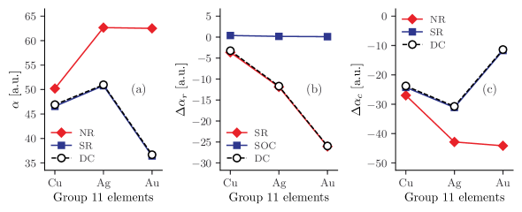
Figure 1: Polarizabilities (in a.u.) of group 11 elements. (a) Comparison of nonrelativistic, scalar-relativistic, and full-relativistic Dirac-Coulomb dipole polarizabilities $\alpha$. (b) Illustration of the influence of relativistic effects, including SR, SOC, and DC, on dipole polarizabilities $\Delta\alpha_{r}$. (c) Examination of the impact of electron-correlation effects on dipole polarizabilities $\Delta\alpha_{c}$ in the presence of various relativistic effects.

V Summary

In this study, we have calculated the static dipole polarizabilities of group 11 elements using the finite-field method combined with relativistic CCSD(T) calculations. Our results showed good agreement with the recommended values from the literature. The final recommended dipole polarizability values, with associated uncertainties, are $46.91\pm 1.30$ for Cu, $50.97\pm 1.88$ for Ag, and $36.68\pm 0.62$ for Au. We also provided a systematic analysis of the impact of various relativistic effects on atomic dipole polarizabilities, including scalar-relativistic effects, SOC, and Dirac-Coulomb relativistic contributions. The analysis indicated that scalar-relativistic effects are the dominant relativistic contribution for Cu, Ag, and Au, while SOC effects were generally negligible. Finally, our investigation of electron correlation, in conjunction with relativistic effects, underscored its critical role in accurately determining the dipole polarizabilities of group 11 elements.