Displaced vertex signals of low temperature baryogenesis

Abstract

We explore the connection of baryogenesis at temperatures below the electroweak scale and signals for long-lived particles at the LHC. The model features new SM singlets, with a long-lived fermion decaying to quarks to generate the baryon asymmetry. The model avoids strong flavor physics bounds while predicting a rich diquark phenomenology, monojet signals, and displaced vertices. We show how the displaced vertex signals can be probed at the HL-LHC. The large transverse production makes a strong physics case for constructing far detector experiments such as MATHUSLA, ANUBIS, and CODEX-b, complementary to the central and forward long-lived particle program.

Introduction  —   The observed matter anti–matter asymmetry remains one of the biggest motivations for physics beyond the standard model (BSM). Some of the traditional BSM baryogenesis mechanisms such as electroweak baryogenesis [1, 2], leptogenesis [3], and Affleck-Dine models [4] generate the baryon asymmetry at high temperatures, above the electroweak (EW) scale, and sometimes much above, e.g. $\sim 10^{15}\operatorname{\text{GeV}}$. While these are well-motivated models, they can be elusive for testing given the high new physics scales involved. Alternatively, low-temperature baryogenesis models propose to generate the baryon asymmetry after the EW transition [5, 6, 7, 8, 9, 10, 11]. To avoid washout effects, baryogenesis occurs via a new particle decaying after sphaleron decoupling and before big bang nucleosynthesis (BBN) times. These decays violate baryon number and generate a CP asymmetry, meeting all three Sahkarov conditions [12].

If a particle $N$ decays to generate the asymmetry, its decay length has to satisfy the out-of-equilibrium condition, $\tau_{N}>H^{-1}$ at temperatures $T\simeq m_{N}$. For masses around the EW scale, this relation implies

$$c\tau_{N}>20~{}\text{mm}\left(m_{N}/100\operatorname{\text{GeV}}\right)^{-2},$$ (1)

resulting in a decay length of macroscopic size. Furthermore, $N$’s lifetime should be larger than a picosecond in order for it to decay after the Sphaleron transition, and smaller than a second for this to occur before BBN. This connection between long-lived particles (LLP) and low-temperature baryogenesis represents an excellent opportunity for displaced vertex searches precisely because they select the decay length window of $0.1\text{mm}\lesssim c\tau_{N}\lesssim 10^{8}\text{m}$. Such signals can be most effectively searched for at the Large Hadron Collider (LHC) and dedicated far detector experiments such as MATHUSLA [13, 14], CODEX-b [15, 16], ANUBIS [17], AL3X [18] and the Forward Physics Facilities [19] with FASER/FASER2 and others.

Figure 1: Diagrams for CP violation in the interference between tree-level and loop decays of $N_{2}$ with and without mixing with the heavier state $N_{3}$. The lightest singlet fermion $N_{1}$ and scalar $\Phi$ are on-shell in the loop to generate a CP asymmetry.

The relationship between LLP and baryogenesis models is surprisingly under-explored in the literature, with only a few proposed models. As reviewed in [14], some of these models are WIMP baryogenesis [20, 21, 22, 23] and baryogenesis via exotic baryon oscillations [24, 25, 26]. In these, charged BSM states enter on-shell in the decay loop amplitude so as to generate CP violation. Because extra SM-charged particles should be heavy, such models prefer masses above the EW scale. Instead, we focus on a lower mass range, $10\operatorname{\text{GeV}}\gtrsim m_{N}\gtrsim 200\operatorname{\text{GeV}}$, resulting in generally longer lifetimes. To reach these masses, we propose a model with only SM singlets below the TeV scale, one of which can successfully decay to create a baryon asymmetry. We combine several features of different models proposed in the literature [27, 28, 29, 30, 31, 32, 33, 34]. The resulting simplified framework naturally avoids proton decay, neutron oscillations, and strong flavor physics bounds while providing a diverse phenomenology for colliders and cosmology. In a companion paper [35], we expand the model to include spontaneous symmetry breaking of baryon number. Here we focus on the model’s aspects that are important for displaced vertices signals.

Model  —  We consider three flavors of singlet Majorana fermions, $N_{\alpha}=N_{{1,2,3}}$, one neutral scalar, $\Phi$, along with new dynamics at a high UV scale. Baryon number violation fixes the dynamics at the UV scale, which generates an effective coupling between $N$ and a neutral combination of quarks. The simplest operator that couples $N$ to SM baryon number happens at dimension six. Since $N$ is neutral, the only quark flavor structure allowed for pairing is $udd^{\prime}$. A minimal possibility that meets these requirements is

$$\operatorname{\mathcal{L}}_{\rm eff}=\frac{\kappa_{\alpha}^{ijk}}{M_{X}^{2}}\big{(}\overline{N_{\alpha}^{c}}u_{R}^{i}\big{)}\big{(}\overline{{d_{R}^{c}}}^{j}d_{R}^{k}\big{)}+\xi_{\alpha\beta}\,\overline{N_{\alpha}^{c}}\Phi N_{\beta}+h.c.$$ (2)

Here, $M_{X}$ is the UV scale, $i,j,k$ are quark generation indices and $\alpha,\beta$ are the neutral fermion flavors. We assume a mass hierarchy of $m_{N_{1}}\lesssim m_{\Phi}<m_{N_{2}}<m_{N_{3}}$. Then, CP violation occurs by the interference between decays with and without mixing of one of the neutral fermions and another heavier state as shown in FIG. 1. A non-zero CP phase requires the mixing term to have on-shell intermediate states in the loop. Therefore, the intermediate states must be lighter than the decaying particle. These requirements show that CP violation occurs exclusively in the decay of $N_{2}$ as it mixes at loop-level with the heavier $N_{3}$ and has an on-shell loop contribution from the lighter $N_{1}$.

The baryon asymmetry parameter is the product of the yield of $N_{2}$, $Y_{2}=\tfrac{n_{N_{2}}}{s}$, the CP asymmetry $\epsilon_{CP}$ and the branching ratio of $N_{2}$ to quarks, $\text{Br}(udd^{\prime})$.

$$Y_{\Delta B}=Y_{2}\epsilon_{CP}\,\text{Br}(udd^{\prime}).$$ (3)

Using the diagrams of FIG. 1, the CP asymmetry is computed to be

$${\epsilon}_{CP}\simeq\frac{6}{16\pi^{2}}\frac{m_{N_{1}}}{m_{N_{3}}}\frac{|\kappa_{2}\kappa_{3}\,\xi_{12}\xi_{13}|\sin\phi}{|\kappa_{2}|^{2}}\sqrt{1-\tfrac{m_{N_{1}}^{2}+m_{\phi}^{2}}{m_{N_{2}}^{2}}}~{},$$ (4)

where $\phi$ is the phase resulting from the coupling product $\kappa_{2}^{ijk}\xi_{12}^{*}\xi_{13}\kappa_{3}^{ijk*}$. We also summed over all quark final states $u,c,d,s,b$ assuming that there are no large flavor hierarchies, which allows us to write $\kappa_{\alpha}^{ijk}\approx\kappa_{\alpha}$ in (4).

To compute $N_{2}$’s yield, we consider the thermal history of the neutral sector. The relevant processes are the annihilation of $N_{2}$ to quarks, $N_{2}u\leftrightarrow dd^{\prime}$, and the decay of $N_{2}\rightarrow udd^{\prime}$. For $m_{N_{2}}\sim 100\operatorname{\text{GeV}}$ with small non-renormalizable interactions, the freeze-out of the annihilation processes can occur when $N_{2}$ is still relativistic, with freeze-out temperature $m_{N_{2}}<T_{FO}<M_{X}$. We can estimate the relativistic freeze-out temperature by setting $n\langle\sigma_{\rm ann}v\rangle\simeq H(T_{FO})$ during radiation domination to get,

$$T_{FO}\simeq 280\operatorname{\text{GeV}}\left(\frac{M_{X}}{2\operatorname{\text{TeV}}}\right)^{4/3}\left(\frac{10^{-6}}{\kappa_{2}}\right)^{2/3}$$ (5)

The relativistic freeze-out of $N_{2}$ is welcome since it maximizes the baryon asymmetry by not having a Boltzmann suppressed population of $N_{2}$. With a sufficiently large lifetime, $N_{2}$ can decay after freeze-out and also after the sphaleron decoupling, avoiding washout from the conversion of baryon to lepton number. Finally, we can obtain the $N_{2}$ yield before decay using the relativistic equilibrium expression

$$Y_{2}=\frac{45\zeta(3)}{2\pi^{4}}\frac{g_{N_{2}}}{g_{*,s}(T_{\rm FO})}~{},$$ (6)

where $g_{N_{2}}$ is the number of $N_{2}$ degrees of freedom, and $g_{*}(T_{FO})$ is the total number of degrees of freedom in the bath at the freeze out temperature.

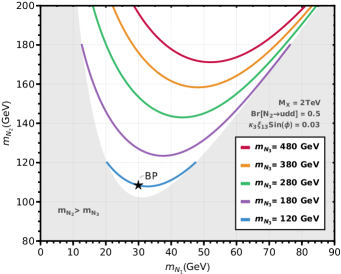
Figure 2: Masses of the particles in the model that reproduce the observed baryon asymmetry. We plot the curves respecting relation (10) in the $m_{N_{1}}\times m_{N_{2}}$ plane. Each curve represents a choice of mass $m_{N_{3}}$ for the scale $M_{X}=2\operatorname{\text{TeV}}$. We choose the values $\kappa_{3}\xi_{13}\sin\phi=0.03$. We assume that $N_{2}$ decays to $u,d,s,c,b$ quarks, with a branching ratio of $0.5$. BP indicates the benchmark point chosen throughout the paper.

Lastly, to compute the branching ratio, we must consider the relative contributions of the tree-body and two-body decays, $N_{2}\rightarrow udd^{\prime}$ and $N_{2}\rightarrow N_{1}\Phi$. For $m_{N_{1}}\sim m_{\Phi}$ the partial decay widths are given by

$$\Gamma_{N_{2}\rightarrow udd^{\prime}}\simeq\frac{6|\kappa_{2}|^{2}}{192\pi^{3}}\frac{m_{N_{2}}^{5}}{M_{X}^{4}},\hskip 17.07182pt\Gamma_{N_{2}\rightarrow N_{1}\Phi}\simeq\frac{m_{N_{2}}|\xi_{12}|^{2}}{\pi}.$$ (7)

Then, the branching ratio of $N_{2}\rightarrow udd^{\prime}$ is

$$\text{Br}(udd^{\prime})\simeq\big{[}32\pi^{2}\left(\xi_{12}/\kappa_{2}\right)^{2}\left(M/m_{N_{2}}\right)^{4}+1\big{]}^{-1}$$ (8)

The decay rate of $N_{2}\rightarrow udd^{\prime}$ should be comparable to $N_{2}\rightarrow N_{1}\Phi$ in order to generate the baryon asymmetry efficiently. In turn, this requirement translates into a relationship between the couplings $\kappa_{2}$ and $\xi_{12}$,

$$\frac{|\xi_{12}|}{|\kappa_{2}|}\approx\frac{1}{4\sqrt{2}\pi}\left(\frac{m_{N_{2}}}{M_{X}}\right)^{2},$$ (9)

where the equality corresponds to a $50\%$ branching ratio to the $udd^{\prime}$ final state. Putting together (4) and (6) and requiring (9) to get a $\mathcal{O}(1)$ branching ratio to the baryon number violating channel, the baryon asymmetry for $M_{X}=2\operatorname{\text{TeV}}$ is given by

$$\frac{Y_{\Delta B}}{Y_{\Delta B}^{\rm exp}}\simeq\left(\frac{m_{N_{2}}}{40\operatorname{\text{GeV}}}\right)^{2}\frac{\kappa_{3}\xi_{13}\sin\phi}{4\times 10^{-2}}\frac{m_{N_{1}}}{m_{N_{3}}}\sqrt{1-\tfrac{m_{N_{1}}^{2}+m_{\phi}^{2}}{m_{N_{2}}^{2}}}$$ (10)

where we used the central value $Y_{\Delta B}^{\rm exp}=8.7\times 10^{-11}$ measured by Planck [36]. In FIG. 2, we impose the measured baryon asymmetry to fix the masses of the $N_{1,2,3}$.

It is useful to define a simple tree-level UV completion for (2) by integrating in a $(\mathbf{3},\mathbf{1})_{2/3}$ SM charged scalar diquark, $X$. The allowed gauge invariant terms are

$$\mathcal{L}_{X}=\lambda_{\alpha i}X^{\dagger}\overline{N^{c}_{\alpha}}u_{R}^{i}+\lambda^{\prime}_{jk}X\overline{d_{R}^{c}}^{j}d_{R}^{k}+h.c.$$ (11)

Such diquark has some interesting low-energy properties. Firstly, if $m_{N_{\alpha}}>1\operatorname{\text{GeV}}$ and $N$ does not mix with neutrinos, the proton does not decay [29]. Secondly, QCD gauge invariance implies color antisymmetry, which means the flavor antisymmetry of the $\overline{d_{R}^{c}}^{j}d_{R}^{k}$ quark couplings in (11). Therefore, there are only three independent $\lambda^{\prime}$ couplings, $\lambda^{\prime}_{jk}=\epsilon_{jkl}\lambda^{\prime}_{l}$. Because of this, there is no tree-level neutron oscillation. The lightest baryon that oscillates is $\Lambda_{0}$, which imposes weak constraints on the diquark mass [35]. Additionally, there are no tree-level $K-\overline{K}$ and $B-\overline{B}$ mixing. At one loop, neutral Kaon mixing must involve the $b$ quark. In the case of B-meson mixing, the loop must contain an $s$ quark. Then, if one of the couplings is small, e.g. $\lambda^{\prime}_{bs}<\lambda^{\prime}_{ds},\lambda^{\prime}_{db}$, then the bounds from meson oscillations can be negligible while still allowing for order one diquark couplings. Assuming $\lambda^{\prime}_{ds}=\lambda^{\prime}_{db}$, Refs. [37, 38, 39, 40, 41] imposed the following constraints from Kaon and B meson oscillations

$$|\lambda^{\prime}_{ds}|~{}\leq~{}3.0\times 10^{-1}~{}\sqrt{M_{X}/2\operatorname{\text{TeV}}},\quad (K-\overline{K}),$$ (12)

$$|\lambda^{\prime}_{db}\lambda^{\prime}_{sb}|\leq 7.2\times 10^{-2}(M_{X}/2\operatorname{\text{TeV}}),\quad (B-\overline{B}~{}).$$ (13)

We can identify the couplings of (11) with (2) as $\kappa_{\alpha}^{ijk}=\lambda_{\alpha i}\lambda^{\prime}_{jk}$. The small value of $\kappa_{2}$, or conversely $\lambda_{2i}$, controls the already suppressed three-body decay of $N_{2}$. Since $N_{1}$ is lighter, its decay length is also macroscopic for a large part of the available parameter space. Therefore, we naturally expect $N_{1,2}$ to be LLPs in the model. In FIG. 3, we show the decay length of $N_{1,2}$ to quarks for various values of the coupling $\lambda_{1i}$ and $\lambda_{2i}$.

LLPs at the LHC  —  Having defined the UV model, we now discuss the LHC sensitivity for the predicted LLPs. We start by considering the direct production bounds on the diquark that govern the necessary UV dynamics of the model. CMS [42, 43] and ATLAS [44] conducted searches for non-resonant pair production of dijet resonances. Their benchmark model is the R-parity-violating supersymmetric top squark that decays to $ds$ quarks and can be directly associated with the diquark $X$ above. The leading limits from [42] excludes the $Y=2/3$ scalar diquark at $95\%$ confidence level between $0.50\operatorname{\text{TeV}}$ and $0.77\operatorname{\text{TeV}}$, with a $3.6(2.5)$ local(global) excess occurring at $0.95\operatorname{\text{TeV}}$. There are also resonant searches for $X$ to a pair of jets conducted by CMS [45, 46] and ATLAS [47] through their diquark couplings. Ref. [40] imposed diquark bounds from resonant production for different values of the coupling pair $(\lambda^{\prime}_{ds},\lambda^{\prime}_{sb})$. For a diquark of mass $M_{X}=2\operatorname{\text{TeV}}$, the values $(\lambda^{\prime}_{ds},\lambda^{\prime}_{sb})=(0.3,0.2)$ are allowed by both direct searches and the flavor constraints of (12) and (13).

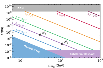
Figure 3: Rest frame decay length of $N_{1,2}$ for different values of the couplings $\lambda_{1,2}$. Avoiding late decays after BBN and early decays before sphaleron decoupling selects the $100~{}\text{$\mu$m}$ to $10^{8}~{}\text{m}$ window for $c\tau$. The CMS monojet search [48] excludes the blue region in the plot.

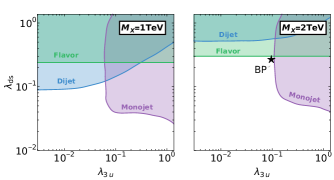
Figure 4: Exclusion bounds for the scalar diquark couplings $(\lambda_{3i},\lambda^{\prime}_{ds})$. CMS [48] constrains the purple monojet region, ATLAS+CMS the blue dijet region, and the flavor bounds come from the meson oscillations in (12) and (13), [37, 40].

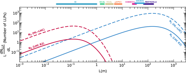
Figure 5: Differential distribution for the number of LLP decays as a function of the distance from the interaction point $L$. The red curve is the number of $N_{2}$ with proper decay length $c\tau_{2}\simeq 1\text{cm}$ and the blue is for $N_{1}$ with $c\tau_{1}\simeq 10\text{m}$. The solid lines are for LHC run 2 (R2) with $\mathcal{L}=139fb^{-1}$, and the dashed are for the high-luminosity phase (HL-LHC) with $\mathcal{L}=3000fb^{-1}$. The color lines above the plot indicate the ATLAS inner detector (ID), the electromagnetic (ECAL) and hadronic calorimeters (HCAL), the muon spectrometer ($\mu$SPEC) and the transverse far experiments CODEX-b, ANUBIS and MATHUSLA.

The production of $N_{\alpha}$ leads to monojet signals when there is a single $X$ or multi-jet plus missing $p_{T}$ for diquark pair production. However, pair production is subdominant for $M_{X}=2\operatorname{\text{TeV}}$ and couplings of $\lambda_{\alpha i}\lesssim 0.3$, and we consider only the monojet channels in our analysis. Moreover, for the monojet channels, $N_{\alpha}$ can be singly produced in the $ds\rightarrow Nu_{i}$ channel or doubly produced by the gluon initiated $gu\rightarrow X^{(*)}N\rightarrow NN^{\prime}u_{i}$ and diquark $t$-channel $u\overline{u}(g)\rightarrow NN^{\prime}(g)$ processes. In the case of the double production $t$-channel, the monojet comes from the initial state emission of a gluon, but these are limited by the high $p_{T}$ cut made in monojet searches. For the other two channels, the resulting $p_{T}$ distribution of the jets is a Jacobian peak at $M_{X}/2$. Because of this feature, the cross-section can be sizable as it does not suffer from the high $p_{T}$ cuts imposed in the monojet analysis. CMS [48] and ATLAS [49] have searched for monojets and monotops in the context of fermion portal dark matter [50] and light non-thermal dark matter models [51]. In FIG. 4, we show the current bounds for the two diquark couplings extracted from [48, 45, 46, 47, 40, 34]. In our model, these bounds are most relevant for $N_{3}$, which is produced and decays promptly to the LLPs. The monojet $N_{3}$ channel is the largest since $\kappa_{3}$ has to be maximized in (3) to get a sizable $Y_{\Delta B}$. Because of this, the monojet $N_{3}$ channel is the one driving our LLP phenomenology, as we discuss next.

Our analysis adopts a single benchmark point shown in the plots with a star labeled BP. We hold the diquark couplings fixed to $(\lambda^{\prime}_{ds},\lambda^{\prime}_{sb})=(0.3,0.2)$. We also choose $\lambda_{1u}=\lambda_{2u}=5\times 10^{-4}$, rendering the lifetimes of $N_{1}$ and $N_{2}$ shown as stars in FIG. 3. The production channel considered is $pp\rightarrow jN_{3}$, with $N_{3}$ decaying to either three $N_{1}$s or one $N_{2}$ and two $N_{1}$s. This happens through the $N_{3}\rightarrow N_{1,2}\Phi$ and $\Phi\rightarrow N_{1}N_{1}$ cascade decay, where we assume the $\Phi$ Yukawa couplings to be $(\xi_{13},\xi_{23})=(1,0.3)$. For the signal simulation, we use MadGraph_aMC@NLO version 2.9.19 with the parton distribution function NNPDF2.3QED and generate the UFO model using FeynRules [52].

	ATLAS/CMS				Transverse Far Detectors			Forward Far Detectors
	ID	ECAL	HCAL	$\mu$SPEC	CODEX-b	ANUBIS	MATHUSLA	FASER/FASER2, …
$N_{\rm obs}$ (Run2)	$<1$	$<1$	$11\times\epsilon_{\rm recon}^{\rm LLP}$	$40\times\epsilon_{\rm recon}^{\rm LLP}$	-	-	-	<1
$N_{\rm obs}$ (HL)	$13$	$23\times\epsilon_{\rm recon}^{\rm LLP}$	$244\times\epsilon_{\rm recon}^{\rm LLP}$	$860\times\epsilon_{\rm recon}^{\rm LLP}$	$27$	$118$	2780	<1

Table 1: Number of observable displaced vertices from the decay of $N_{1,2}\rightarrow udd^{\prime}$ inside the inner detector (ID), electromagnetic and hadronic calorimeters (ECAL and HCAL), and muon spectrometers($\mu$SPEC). We assume the large-tracking radius algorithm of [53] to estimate the efficiency of LLP reconstruction for decays inside the ID and optimistically choose $\epsilon_{\rm recon}^{\rm LLP}=1$ for far detectors. The number of events inside the ECAL/HCAL and $\mu$SPEC is left as a function of reconstruction efficiency.

We extract the angular and velocity distribution of $N_{1}$ and $N_{2}$ from the simulated data. The majority of events are transverse to the interaction plane, forming an approximately uniform angular distribution for $|\eta|<5$. From the velocity distribution, we can extract the boosted lifetimes $\beta\gamma c\tau$, and construct the differential probability distribution for $N_{1,2}$ to decay at position $L$,

$$\frac{d\mathcal{P}_{\rm dec}(L)}{dL}=\frac{e^{-\frac{L}{\beta\gamma c\tau_{i}}}}{\beta\gamma c\tau_{i}}.$$ (14)

Then, the differential number of events observed as a function of the distance $L$ is given by

$$\frac{dN_{\rm obs}}{dL}=\overbrace{(n\sigma\mathcal{L})\otimes\text{Br}(udd^{\prime})\otimes\frac{d\mathcal{P}_{\rm dec}}{dL}}^{\equiv dN_{\rm dec}/dL}\otimes\xi_{geom}^{\rm LLP}\otimes\epsilon_{recon}^{LLP},$$ (15)

where $n$ is the multiplicity of $N_{1,2}$ of the process, $\mathcal{L}$ is the luminosity, $\xi_{geom}^{LLP}$ is the geometric acceptance of the experiment and $\epsilon_{recon}^{LLP}$ is the efficiency of reconstruction of the displaced vertices. In FIG. 5, we obtain the differential number of LLP decays defined in the overbrace of (15) as a function of the distance $L$. Notice that the value obtained is for the whole solid angle without specifying the geometric acceptance and detector efficiencies. The number of displaced vertices is sizable in several regions of the future LHC experiments, as well as for proposed far detectors with sensitivity to transverse events. To get an estimate of the number of LLPs in each experiment, we can integrate the length $L$ in (14) to obtain the decay probability inside a detector that starts at $L_{\rm in}$ and ends at $L_{\rm fin}$,

$$\mathcal{P}_{\rm dec}=e^{-\frac{\rm L_{\rm in}}{\beta\gamma c\tau_{i}}}-e^{-\frac{L_{\rm fin}}{\beta\gamma c\tau_{i}}}.$$ (16)

In TABLE 1, we estimate the number of events for the benchmark point used throughout the paper for various LHC experiments during run 2 and the HL-LHC. For decays inside the inner detector of the ATLAS experiment, we assume the large-radius tracking reconstruction algorithm used in a similar search for RPV SUSY long-lived neutralinos [53]. There are also displaced decays inside the calorimeters and muon spectrometers of the ATLAS/CMS experiments. However, we are not aware of a reconstruction strategy for the three-jet signals of the LLPs of our model beyond the ID. Because of that, we show the resulting number of events without specifying the reconstruction efficiencies of each part of the detector. For the far detectors, we consider the transverse and forward experiments CODEX-b, ANUBIS, MATHUSLA, and FASER/FASER2. To obtain the geometric acceptances, we integrate the number of events distribution over the solid angle covered by each experiment, approximating the total volume by using the midpoint of the detector to define the angular cone and integrating from $L_{\rm in}$ to $L_{\rm fin}$ for each detector. We choose the optimistic scenario by assuming that the reconstruction efficiencies of the far detectors are $\epsilon_{\rm recon}^{\rm LLP}=1$. While the forward far detectors have negligible event rates due to the limited solid angle coverage, the transverse detectors present a significant sensitivity to LLP decays. This enhanced sensitivity is primarily due to their optimal positioning relative to the interaction point, which allows for a larger geometric acceptance and increased event visibility. As shown in FIG. 5, the experiments considered are complementary in their range for probing $c\tau$. The ATLAS/CMS inner detectors are more efficient for searching for $N_{2}$, which is generally less long-lived than $N_{1}$. CODEX-b, ANUBIS and MATHUSLA are strategically positioned at successive distances from the interaction point, allowing for a continuous probing of the region ranging from $26$ to $170$ meters. We leave for future work a more in-depth analysis of the HL-LHC predictions of each experiment and a scan over the parameters of the model. However, from our current estimates, the HL-LHC presents an interesting scenario for probing the model, presenting a strong physics case for the construction of the transverse far detectors mentioned above.

Conclusions  —  In this paper, we explore the connection of baryogenesis through out-of-equilibrium decays at low temperatures and the detection of long-lived particles at the LHC. The proposed model can be probed through the detection of LLPs and associated phenomenology using current and future LHC experiments. The model minimally requires the presence of three flavors of majorana fermions $N_{1,2,3}$, a neutral scalar $\Phi$, and some $\operatorname{\text{TeV}}$ scale dynamics which we assume to be related to a scalar diquark with $2/3$ hypercharge. The model avoids proton decay because $N$ does not mix with neutrinos, has no tree-level neutron oscillations, and has small loop-suppressed $\Delta F=2$ neutral meson oscillations. At the same time, there are plenty of interesting collider signals ranging from the detection of the diquarks to monojet signals with missing energy and displaced vertices, which are the main focus of the paper. The HL-LHC provides a promising scenario for probing the model as a significant number of LLPs can be produced, as illustrated in FIG. 5 and TABLE 1. Transverse far detectors like CODEX-b, ANUBIS, and MATHUSLA have a significantly higher sensitivity to LLP decays compared to forward detectors due to their optimal positioning and larger geometric acceptance. The increased sensitivity of transverse far detectors highlights the importance of their construction and complementary ability to probe new physics at the HL-LHC.

- [1] A.G. Cohen, D.B. Kaplan and A.E. Nelson, Progress in electroweak baryogenesis, Ann. Rev. Nucl. Part. Sci. 43 (1993) 27 [hep-ph/9302210].
- [2] C.E.M. Wagner, Electroweak Baryogenesis and Higgs Physics, LHEP 2023 (2023) 466 [2311.06949].
- [3] S. Davidson, E. Nardi and Y. Nir, Leptogenesis, Phys. Rept. 466 (2008) 105 [0802.2962].
- [4] R. Allahverdi and A. Mazumdar, A mini review on Affleck-Dine baryogenesis, New J. Phys. 14 (2012) 125013.
- [5] S. Dimopoulos and L.J. Hall, Baryogenesis at the MeV Era, Phys. Lett. B 196 (1987) 135.
- [6] M. Trodden, Making baryons below the electroweak scale, in 3rd International Conference on Particle Physics and the Early Universe, pp. 398–404, 2000, DOI [hep-ph/0001026].
- [7] K.S. Babu, R.N. Mohapatra and S. Nasri, Post-Sphaleron Baryogenesis, Phys. Rev. Lett. 97 (2006) 131301 [hep-ph/0606144].
- [8] K.S. Babu, R.N. Mohapatra and S. Nasri, Unified TeV Scale Picture of Baryogenesis and Dark Matter, Phys. Rev. Lett. 98 (2007) 161301 [hep-ph/0612357].
- [9] K. Kohri, A. Mazumdar and N. Sahu, Inflation, baryogenesis and gravitino dark matter at ultra low reheat temperatures, Phys. Rev. D 80 (2009) 103504 [0905.1625].
- [10] R. Allahverdi, B. Dutta and K. Sinha, Baryogenesis and Late-Decaying Moduli, Phys. Rev. D 82 (2010) 035004 [1005.2804].
- [11] R. Allahverdi, N.P.D. Loc and J.K. Osiński, Dark matter and baryogenesis from visible-sector long-lived particles, Phys. Rev. D 107 (2023) 123510 [2212.11303].
- [12] A.D. Sakharov, Violation of CP Invariance, C asymmetry, and baryon asymmetry of the universe, Pisma Zh. Eksp. Teor. Fiz. 5 (1967) 32.
- [13] MATHUSLA collaboration, An Update to the Letter of Intent for MATHUSLA: Search for Long-Lived Particles at the HL-LHC, 2009.01693.
- [14] D. Curtin et al., Long-Lived Particles at the Energy Frontier: The MATHUSLA Physics Case, Rept. Prog. Phys. 82 (2019) 116201 [1806.07396].
- [15] G. Aielli et al., The Road Ahead for CODEX-b, 2203.07316.
- [16] V.V. Gligorov, S. Knapen, M. Papucci and D.J. Robinson, Searching for Long-lived Particles: A Compact Detector for Exotics at LHCb, Phys. Rev. D 97 (2018) 015023 [1708.09395].
- [17] M. Bauer, O. Brandt, L. Lee and C. Ohm, ANUBIS: Proposal to search for long-lived neutral particles in CERN service shafts, 1909.13022.
- [18] V.V. Gligorov, S. Knapen, B. Nachman, M. Papucci and D.J. Robinson, Leveraging the ALICE/L3 cavern for long-lived particle searches, Phys. Rev. D 99 (2019) 015023 [1810.03636].
- [19] J.L. Feng et al., The Forward Physics Facility at the High-Luminosity LHC, J. Phys. G 50 (2023) 030501 [2203.05090].
- [20] Y. Cui and R. Sundrum, Baryogenesis for weakly interacting massive particles, Phys. Rev. D 87 (2013) 116013 [1212.2973].
- [21] Y. Cui, Natural Baryogenesis from Unnatural Supersymmetry, JHEP 12 (2013) 067 [1309.2952].
- [22] Y. Cui and B. Shuve, Probing Baryogenesis with Displaced Vertices at the LHC, JHEP 02 (2015) 049 [1409.6729].
- [23] Y. Cui, T. Okui and A. Yunesi, LHC Signatures of WIMP-triggered Baryogenesis, Phys. Rev. D 94 (2016) 115022 [1605.08736].
- [24] S. Ipek and J. March-Russell, Baryogenesis via Particle-Antiparticle Oscillations, Phys. Rev. D 93 (2016) 123528 [1604.00009].
- [25] K. Aitken, D. McKeen, T. Neder and A.E. Nelson, Baryogenesis from Oscillations of Charmed or Beautiful Baryons, Phys. Rev. D 96 (2017) 075009 [1708.01259].
- [26] D. McKeen and A.E. Nelson, CP Violating Baryon Oscillations, Phys. Rev. D 94 (2016) 076002 [1512.05359].
- [27] H. Davoudiasl, D.E. Morrissey, K. Sigurdson and S. Tulin, Hylogenesis: A Unified Origin for Baryonic Visible Matter and Antibaryonic Dark Matter, Phys. Rev. Lett. 105 (2010) 211304 [1008.2399].
- [28] H. Davoudiasl and Y. Zhang, Baryon Number Violation via Majorana Neutrinos in the Early Universe, at the LHC, and Deep Underground, Phys. Rev. D 92 (2015) 016005 [1504.07244].
- [29] J.M. Arnold, B. Fornal and M.B. Wise, Simplified models with baryon number violation but no proton decay, Phys. Rev. D 87 (2013) 075004 [1212.4556].
- [30] N. Assad, B. Fornal and B. Grinstein, Baryon Number and Lepton Universality Violation in Leptoquark and Diquark Models, Phys. Lett. B 777 (2018) 324 [1708.06350].
- [31] C. Cheung and K. Ishiwata, Baryogenesis with Higher Dimension Operators, Phys. Rev. D 88 (2013) 017901 [1304.0468].
- [32] R. Allahverdi, B. Dutta and K. Sinha, Cladogenesis: Baryon-Dark Matter Coincidence from Branchings in Moduli Decay, Phys. Rev. D 83 (2011) 083502 [1011.1286].
- [33] R. Allahverdi and B. Dutta, Natural GeV Dark Matter and the Baryon-Dark Matter Coincidence Puzzle, Phys. Rev. D 88 (2013) 023525 [1304.0711].
- [34] R. Allahverdi, P.S.B. Dev and B. Dutta, A simple testable model of baryon number violation: Baryogenesis, dark matter, neutron–antineutron oscillation and collider signals, Phys. Lett. B 779 (2018) 262 [1712.02713].
- [35] P. Bittar, G. Burdman and G.M. Salla, Spontaneous breaking of baryon number, baryogenesis and the bajoron, 2410.00964.
- [36] Planck collaboration, Planck 2018 results. VI. Cosmological parameters, Astron. Astrophys. 641 (2020) A6 [1807.06209].
- [37] G.F. Giudice, B. Gripaios and R. Sundrum, Flavourful Production at Hadron Colliders, JHEP 08 (2011) 055 [1105.3161].
- [38] T. Han, I. Lewis and Z. Liu, Colored Resonant Signals at the LHC: Largest Rate and Simplest Topology, JHEP 12 (2010) 085 [1010.4309].
- [39] I. Baldes, N.F. Bell and R.R. Volkas, Baryon Number Violating Scalar Diquarks at the LHC, Phys. Rev. D 84 (2011) 115019 [1110.4450].
- [40] B. Pascual-Dias, P. Saha and D. London, LHC Constraints on Scalar Diquarks, JHEP 07 (2020) 144 [2006.13385].
- [41] T. Han, I.M. Lewis, H. Liu, Z. Liu and X. Wang, A Guide to Diagnosing Colored Resonances at Hadron Colliders, 2306.00079.
- [42] CMS collaboration, Search for resonant and nonresonant production of pairs of dijet resonances in proton-proton collisions at = 13 TeV, JHEP 07 (2023) 161 [2206.09997].
- [43] CMS collaboration, Search for pair-produced resonances decaying to quark pairs in proton-proton collisions at 13 TeV, Phys. Rev. D 98 (2018) 112014 [1808.03124].
- [44] ATLAS collaboration, A search for pair-produced resonances in four-jet final states at 13 TeV with the ATLAS detector, Eur. Phys. J. C 78 (2018) 250 [1710.07171].
- [45] CMS collaboration, Search for narrow and broad dijet resonances in proton-proton collisions at TeV and constraints on dark matter mediators and other new particles, JHEP 08 (2018) 130 [1806.00843].
- [46] CMS collaboration, Search for high mass dijet resonances with a new background prediction method in proton-proton collisions at 13 TeV, JHEP 05 (2020) 033 [1911.03947].
- [47] ATLAS collaboration, Search for new resonances in mass distributions of jet pairs using 139 fb-1 of collisions at TeV with the ATLAS detector, JHEP 03 (2020) 145 [1910.08447].
- [48] CMS collaboration, Search for new physics in final states with an energetic jet or a hadronically decaying W or Z boson using of data at , .
- [49] ATLAS collaboration, Search for invisible particles produced in association with single top quarks in proton-proton collisions at =13 TeV with the ATLAS detector, 2402.16561.
- [50] Y. Bai and J. Berger, Fermion Portal Dark Matter, JHEP 11 (2013) 171 [1308.0612].
- [51] B. Dutta, Y. Gao and T. Kamon, Probing Light Nonthermal Dark Matter at the LHC, Phys. Rev. D 89 (2014) 096009 [1401.1825].
- [52] A. Alloul, N.D. Christensen, C. Degrande, C. Duhr and B. Fuks, FeynRules 2.0 - A complete toolbox for tree-level phenomenology, Comput. Phys. Commun. 185 (2014) 2250 [1310.1921].
- [53] ATLAS collaboration, Search for long-lived, massive particles in events with displaced vertices and multiple jets in pp collisions at = 13 TeV with the ATLAS detector, JHEP 2306 (2023) 200 [2301.13866].