Monte Carlo Simulation of Operator Dynamics and Entanglement
in Dual-Unitary Circuits
Abstract
We investigate operator dynamics and entanglement growth in dual-unitary circuits, a class of locally scrambled quantum systems that enables efficient simulation beyond the exponential complexity of the Hilbert space. By mapping the operator evolution to a classical Markov process, we perform Monte Carlo simulations to access the time evolution of local operator density and entanglement with polynomial computational cost. Our results reveal that the operator density converges exponentially to a steady-state value, with analytical bounds that match our simulations. Additionally, we observe a volume-law scaling of operator entanglement across different subregions, and identify a critical transition from maximal to sub-maximal entanglement growth, governed by the circuit’s gate parameter. This transition, confirmed by both mean-field theory and Monte Carlo simulations, provides new insights into operator entanglement dynamics in quantum many-body systems. Our work offers a scalable computational framework for studying long-time operator evolution and entanglement, paving the way for deeper exploration of quantum information dynamics.
I Introduction
In quantum many-body physics, the study of operator dynamics is an active area of research. The dynamics of quantum operators under Heisenberg picture time evolution can provide insights into the complex behavior of quantum many-body systems, including operator spreading [1, 2, 3, 4, 5, 6, 7, 8, 9, 10], scrambling and thermalization [11, 12, 13, 14, 15, 16, 17, 18, 19, 20, 21]. Simulating operator dynamics in quantum many-body systems is generally challenging due to the curse of dimensionality—the exponential growth of the Hilbert space with system size. While efficient computational methods exist in specific cases, such as Clifford circuits [22], time-evolving block decimation (TEBD) [23, 24, 25], or systems with partial integrability [26, 27], a general solution remains elusive.
When focusing solely on the statistical properties of operator dynamics, i.e. how the size and support of an operator evolves on average without concern for the specific operator content, more efficient approaches become available [3, 28, 4, 7, 29]. For locally scrambled quantum dynamics [15, 16], where the unitary evolution operators are weakly symmetric [30, 31] under local basis transformations, the operator dynamics can be mapped to an effective classical diffusion model in the space of operator supports [3, 29, 32]. This mapping simplifies the quantum evolution into a tractable classical Markov process, allowing for efficient simulation via Monte Carlo (MC) sampling.
Furthermore, to characterize the internal complexity and correlations within an operator, the concept of operator entanglement has been introduced [33, 34, 35, 36]. Operator entanglement quantifies the entanglement of the corresponding Choi state representation [37, 38] of the operator in the operator Hilbert space (a.k.a. doubled Hilbert space). In the context of operator dynamics, it characterizes how the information encoded by the initial operator scrambles with time and becomes correlated across different parts of the system over time. Nicely, we found that the second Rényi operator entanglement can also be studied under reasonable assumptions using above-mentioned Monte Carlo approach for operator dynamics on multiple replicas, enabling efficient computation of these quantities in complex systems.
In this work, we investigate the operator dynamics and operator entanglement in dual-unitary circuits — a class of quantum circuits consisting of dual-unitary gates, which are unitary in both space and time directions [39, 36, 35]. Dual-unitary circuits, like Haar random unitary circuits, are examples of locally scrambled quantum dynamics that enable operator dynamics to be studied efficiently by mapping to classical diffusion processes. However, compared to Haar random unitary gates, dual-unitary gates form a family of random unitary ensembles with tunable scrambling power controlled by a single parameter. This tunability allows us to systematically explore different scrambling behaviors within the same theoretical framework.
We demonstrate, via Monte Carlo simulations of the local operator density and entanglement in a dual-unitary circuit, that the operator density near the light cone converges exponentially to , with a rate determined by the gate parameter . In the long-time limit, we derive analytical bounds for the density profile, validated by Monte Carlo simulations. For operator entanglement, we observe volume-law scaling across different subregions, with the volume-law coefficient’s dependence on varying. A key finding is the transition from maximal to sub-maximal entanglement growth for left movers at the left light cone, consistent with prior theoretical work [39, 36, 35, 40]. Our study provides a direct mapping of the volume-law coefficient to , confirmed by mean-field (MF) theory and Monte Carlo simulations, offering new insights into operator dynamics and entanglement transitions in dual-unitary circuits.
II Locally-scrambled Dual-unitary Dynamics
To introduce the concept of a dual-unitary gate, we consider an arbitrary two-qubit gate . In the computational basis, its space-time dual can be defined as
| (1) |
The unitary is called dual-unitary when its space-time dual is also a unitary operator, satisfying [39]. For qubit systems, dual unitary gates are parameterized by four single-qubit unitaries , , and a single parameter :
| (2) |
Here, are the Pauli operators on the -th qubit. Single-qubit gates provide local basis rotations but do not entangle different sites. The non-trivial entanglement arises from the XXZ coupling, where characterizes the scrambling ability of the dual-unitary gate. For , reduces to a SWAP operation, simply interchanging operators between two sites. Conversely, for , it maximally spreading single-site operators to operators supported on both sites.
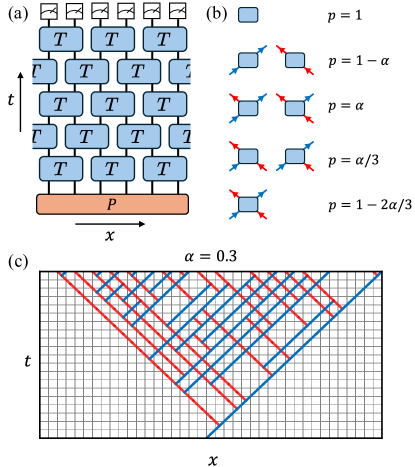
In this work, we study the operator dynamics of random dual-unitary circuits for qubit systems arranged in a brick-wall architecture, as shown in Fig. 1 (a). The evolution operator is given by , where
| (3) |
Here, represent two-qubit dual-unitary gates acting on nearest-neighbor qubits and . We note that throughout this paper, we use to denote the quantum evolution operator and the transfer matrix after mapping the dual-unitary quantum circuit to the classical Markov process. We sample each two-qubit gate independently in the locally-scrambled dual-unitary ensemble from the distribution condition on the parameter , and define the random unitary ensemble :
| (4) |
where and represent the Haar measure of single-qubit rotations. This choice eliminates local basis dependence and is essential to mapping the full quantum dynamics to a classical Markov process [15], which then admits efficient Monte Carlo simulations, as we showed in this paper.
We are interested in the dynamical evolution of simple operators . At time , the Heisenberg evolution is given by . For later convenience, we represent the operator as a state in a doubled Hilbert space, known as the Choi representation [37, 38]. On a complete set of orthonormal basis of the Hilbert space, under the operator-state mapping, any generic operator gets mapped to a corresponding doubled state as . Here, denotes the system size. In this language, the Heisenberg evolution reads . We choose a orthogonal basis in the operator space at site as , where each basis state corresponds to having the operator acting on the qubit , respectively. The operator wavefunction can be expanded as
| (5) |
where with . We study the growth of a local operator that initially acts near the middle of the system (around ), focusing on the time regime before it reaches the system boundaries under the operator dynamics, so that boundary effects remain irrelevant.
II.1 Operator Density
We investigate the operator dynamics by monitoring both the evolution of operator density [3] and the operator entanglement entropy [36]. The operator density is defined as the probability of finding a non-trivial operator on site :
| (6) |
Here, the overline denotes the ensemble average over the realizations of random single-qubit gates in the dual-unitary ensemble. There are great simplications if we focus on locally-scrambled quantum circuits: the phase of exhibits random fluctuations due to the random single-qubit rotations, and the evolution of becomes Markovian [15]. The evolution generated by each two-qubit gate reads
| (7) |
where the summation is restricted to the subspace where for any . The 1616 transfer matrix is computed in a two-qubit system by
| (8) | ||||
The completeness of Pauli operators guarantees the conservation of the probability, as .
Furthermore, we observe that the absence of local basis dependence suggests that only depends on the support of and . As a consequence, at also depends only on the support of rather than on the specific content of the Pauli string . To eliminate the redundancy in , we introduce a bit string to denote the support of a Pauli string, where . We use to indicate the case where the site is not occupied by the operator and for the occupied case. Then, we can rewrite the Markov process in this occupation basis, where the transfer matrix can be reduced to a matrix . Introduce , where is an arbitrary Pauli operator of support , with denoting the number of occupied sites in the bit string (i.e. the operator size), and the factor counts the total number of Pauli operators of the same support . The operator density can be expressed as
| (9) |
Defining , the evolution generated by each two-qubit gate remains
| (10) |
where the summation is again restricted to the subspace where for any . The full Markovian dynamics is then represented by a brick-wall circuit of local transfer matrices , as illustrated in Fig. 1 (a). For the locally-scrambled dual-unitary ensemble, the explicit expression of for each two-qubit gate has been computed [40], which reads
| (11) |
with parametrization that controls the information scrambling power of the dual-unitary gate ensemble: corresponds to the SWAP gate with no scrambling, and corresponds to the fastest scrambling dual unitary gates.
II.2 Operator Entanglement
We also examine the growth of operator entanglement in the random dual-unitary circuit [36, 35]. After mapping the operator to a state, the operator entanglement for a subregion of the original qubit system is defined as the conventional entanglement entropy of the corresponding Choi state for the same subregion, as illustrated in Fig. 2.
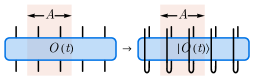
More explicitly, we first construct the reduced density matrix in the operator space
| (12) |
Here, denotes the complement of the subregion . We can compute either the von Neumann entropy or the -th Rényi entropy . In this work, we focus on small subsystem size , where theoretical analysis becomes more tractable after the following approximations regarding the disorder average:
| (13) | ||||
In the first step, we approximate the disorder average of the entropy by the disorder average of . This approximation assumes that the corresponding variance is negligible within the ensemble of random circuits [41, 42]. However, the calculation still requires the disorder average over 2-replicas , where the Schur-Weyl duality suggests that the effective degrees of freedom are elements of the group. To further simplify the calculation, we assume that is dominated by the “replica diagonal” contribution for small subsystems , allowing us to replace with , which constitutes our second step. It is known that these approximations become exact if we consider a system with qudits and take the limit of a large local Hilbert space dimension [36].
Under this approximation, we can express the second Rényi entropy in terms of . As explained in Sec. II.1, the disorder-averaged operator density matrix contains only the diagonal components: Tracing out the subregion , we obtain the reduced density matrix
| (14) |
where we have decomposed and introduced the marginal distribution . The purity of the system is then computed by
| (15) |
where denotes a bit string defined in region .
II.3 Monte Carlo Simulation
Since contains an exponentially large number of components, indexed by the bit string (with ) that labels the operator support. Direct analytical or numerical study of the evolution of following Eq. (10) is impractical. To this end, we would like to use the Monte Carlo method to carry out important sampling and reduce the exponential computation to polynomial complexity. We may interpret the operator support as an occupation configuration of some fictitious “particles”, and visualize the Markovian dynamics of operator evolution as the evolution of classical particles, where each lattice site is either empty () or occupied by a particle (). The system is initialized according to the support of the initial operator . The application of a transfer matrix in Eq. (11) on sites and is then implemented by the following local update rule, parametrized by the scrambling parameter of the dual unitary gate:
-
1.
If both sites are unoccupied, no update is needed.
-
2.
If only site is occupied, we move the particle from site to site . With a probability of , site is left empty. Otherwise, a new particle is added at site .
-
3.
If only site is occupied, we move the particle from site to site . With a probability of , site is left empty. Otherwise, a new particle is added at site .
-
4.
If both sites are occupied, the configuration is kept unchanged with a probability . Otherwise, one of the two particles is randomly removed, and the probability to remove either particle is .
These update rules are graphically shown in Fig. 1 (b) and they reveal a central feature of dual-unitary circuits with a brick-wall architecture. In the absence of scattering with other particles, a particle continues to move in a single spatial direction. Therefore, it is natural to distinguish lattice sites corresponding to right movers and left movers based on the parity of . As an illustration, we depict right movers in blue and left movers in red in Fig. 1 (c) for a typical evolution history.
Starting from any initial configuration of the operator support (equivalently viewed as “particle” occupation configuration) at time , we can stochastically generate the configuration at later time following the update rules described above. These update rules ensure that the underlying probability distribution of at time will precisely match , as if we can effectively sample from the distribution .
After collecting many independent samples, we can estimate the operator density by counting the average particle number at the corresponding space-time position. On the other hand, the operator entanglement entropy is a non-linear function of the probability distribution . In the Monte Carlo simulation, we focus on the second Rényi entropy with Rényi index . This first requires generating two independent configurations of classical particles at time , labeled by their occupation bit strings and . Then, we compute
| (16) |
as an estimator of Eq. (15). Here, is the Kronecker delta symbol that enforces and have identical configurations inside the entanglement region of interest, otherwise the quantity will be zero. Averaging over many pairs of samples gives , and then .
As one can see from Eq. (16), a non-zero is sampled only if , which is an exponentially rare event to happen. This makes the sampling exponentially inefficient for estimating the operator entanglement. In practice, we mitigate this issue by computing the probability distribution at time condition on the configuration generated at time , where denotes the time slice where operator properties are measured. Recall that each local transfer matrix acts on one pair of left and right movers, and is unrelated to the others pair of movers in the same time slice due to the brick-wall architecture. Therefore, for every two sites (a pair of movers), we can explicitly compute the probability of all four possible states in the 2-site state space occurring at , conditioned on the current state at . Let’s denote the particle configuration at time by the bit string , and that at time by the bit string . Then we can compute the quantity as a function of and , which are independently sampled in two replica up to the time step,
| (17) |
which amounts to directly summing over all the final-time configurations based on the conditional probability . Here corresponds to the conditional probability to generate given in a single replica, which is given by (the tensor product) of the transfer matrix , defined in Eq. (11),
| (18) |
assuming the last time step is an odd step without lost of generality. In this way, averaging also gives unbiased estimation of the operator entanglement . Since the summation of configurations can be factorized to that on each pair of sites at , which can computed efficiently, we can now obtain a finite real number from each Monte Carlo sampling instead of waiting an exponentially long time for to occur. Similar approach in spirit, to overcome the exponential observable with log-normal distribution to a typical observable with normal distribution [43, 44, 45], has been employed in the recent computation of entanglement entropy and other exponential observables in the quantum many-body systems within quantum Monte Carlo and Tensor Network setup [46, 47, 48, 49, 50, 51, 52, 53, 44].
III Results
In the following, we will investigate the operator dynamics and operator entanglement growth in dual-unitary circuits using the Monte Carlo sampling approach described above, and compare the results with mean-field theoretical understandings.
For the operator dynamics, we focusing on two initial operators: and . For , we find that the operator density evolution closely follows the mean-field approximation, with our analytical solutions in both the long-time limit and near the light-cone matching well with Monte Carlo simulations. Conversely, for , the operator density near the left light-cone deviates significantly from mean-field predictions due to strong correlations arising from the stochastic emission time of the first left-moving operator. By incorporating a conditional probability framework, we derive analytical expressions that accurately capture these correlations, achieving excellent agreement with numerical results.
Additionally, we explore operator entanglement growth in three different subregions near the light-cone and identify entanglement transitions as the parameter varies. Our analytical predictions of critical values for these transitions are validated by Monte Carlo simulations, which has not been observed in previous works [39, 36, 35, 40]. Our discovery therefore highlights the sensitivity of entanglement growth to initial conditions and system parameters.
Overall, our findings demonstrate the intricate interplay between operator dynamics, correlations, and entanglement scaling in dual-unitary circuits, enhancing the understanding of information spreading, thermalization, and quantum information scrambling in quantum many-body systems.
III.1 Operator Density Evolution
We begin with the analysis of operator density evolution. For illustration, we focus on two different initial operators: (two-site operator) or (single-site operator), which turns out to show different features. According to our convention in Eq. (3), represents a left mover, while corresponds to a right mover. We present typical results of the operator density evolution in Fig. 3 (a) and (b) using solid lines for and . The data presented is averaged over Monte Carlo steps such that error bars are negligible from bare-eye observation.
III.1.1 Balanced operator growth from two-site operator
Let us first focus on the scenario with . On both the left () and right () light-cones, the operator density is 1, consistent with the ballistic transport of the initial operator. Within this light-cone, the operator density continues to increase due to the creation of new particles at finite splitting probability . In the long-time limit, the operator density on each site approaches , indicating that each single-qubit Pauli operator appears with equal probability, as expected for generic chaotic quantum systems [54]. To gain a more quantitative understanding, we adopt the zeroth-order mean-field approximation [40], which approximates the joint distribution of the operator support as product of independent Bernoulli distribution of on each site , parametrized by the operator density as
| (19) |
This mean-field approximation neglects any correlation between different sites. The evolution of is then derived by applying a layer of transfer matrix and computing the post-evolution density [40]. For a transfer matrix applied to sites and , the evolution reads
| (20) | ||||
The evolution generated by these equations is plotted in Fig. 3 (a) using dashed lines. The results match the Monte Carlo simulation with high accuracy for . Additionally, we provide analytical solutions in two limits:
-
1.
In the long-time limit for a fixed lattice site , we can neglect the spatial dependence of the operator density and expand . The evolution then becomes
(21) This equation can be solved exactly, which gives
(22) -
2.
Now, we consider the near-light-cone steady state for the operator density. Specifically, we examine the case where or with . Numerical results suggest the existence of a steady-state distribution , where LC stands for “light-cone”, which satisfies , and
(23) Using the first equation, we find
(24) for any . Substituting this into the second equation, we have ()
(25)
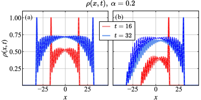
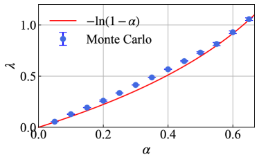
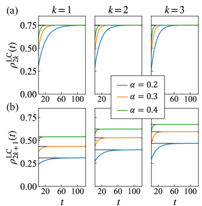
We test both predictions through the Monte Carlo sampling of the at various for . Since becomes spatially independent at , we focus on the density evolution at without loss of generality. By fitting the density evolution with Eq. (22), we find an exponential growth coefficient that is consistent with the analytical solution in Eq. (22), as shown in Fig. 4. For the near-light-cone steady state, MC data of both and exponentially converges to the MF prediction in Eq. (25) at large-enough , as exemplified in Fig. 5 (a) and (b) for at .
III.1.2 Skewed operator growth from single-site operator
We then consider the operator density evolution for , as shown in Fig. 3 (b). In this case, the right light-cone () has an operator density of 1, while the density on the left light-cone is , determined by the probability of operator emission at the first step. Unlike the previous example with , numerical results show that the operator density evolution near the left light-cone differs significantly from a direct mean-field solution. This discrepancy arises because the mean-field analysis is valid only when the operator occupations on different sites are nearly independent, allowing correlations to be neglected. However, strong correlations exist near the left light-cone for , and this can be explained in the following way.
We consider the conditional probability of the full operator dynamics, where labels the time when the initial operator emits a left mover for the first time. This left mover becomes the leftmost particle and will never disappear in subsequent evolution. The probability distribution of is given by
| (26) |
After the emission of the first left mover, we have two nearest neighbor particles, and the evolution of operator density matches previous discussions for . This results in
| (27) |
Here, is the operator density for . Specifically, we have if and if , indicating a long-range correlation between different sites near the left light-cone after summing up contributions from different . Therefore, a naive mean-field theory does not apply. However, since it has been established that can be described by the mean-field equation, we can still make predictions using a superposition of mean-field results:
| (28) |
Since exponentially localizes at small , evident from Eq. (26), it does not change the long-time relaxation to and the steady-state operator density near the right light-cone, which is still given by Eq. (25). For the steady-state near the left light-cone, the dependence on becomes significant. Defining , we have ,
| (29) | ||||
and
| (30) | ||||
for any .
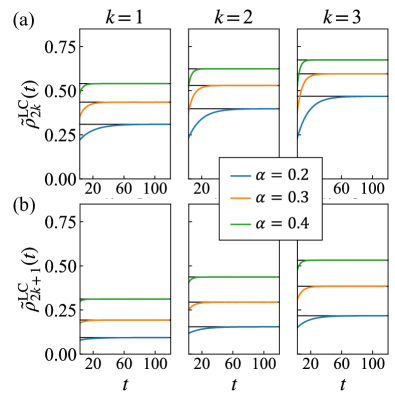
Again, we test the above prediction near the left light-cone with initial condition by directly comparing with Monte Carlo simulations, as exemplified in Fig. 6 (a) and (b) for at . The operator density near the left light-cone for both left and right movers converges to the mean-field results in Eqs. (29) and (30) as increases.
III.1.3 Summary of results on operator density
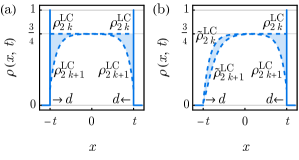
In this subsection, we investigated the operator growth dynamics in dual-unitary circuits with a brick-wall arrangement of two-qubit gates, characterized by the gate parameter . Near the center of the light cone of the growing operator, the operator density converges exponentially to , following , with the rate determined by . In the long-time limit, the operator density will converge to the profile depicted in Fig. 7, which oscillates between upper and lower bounds. We derived analytical expressions for these bounds based on a mean-field-like theory, where operators spread like diffusive “particles”, and correlations among these particles are retained only to the minimal necessary order. Their expressions and verifications are summarized in the table within Fig. 7.
III.2 Operator Entanglement Growth
Next, we study the dynamics of operator entanglement, focusing on the steady-state entanglement for subregions near the light-cone starting from the single-site operator . As established in Sec. III.1, the results obtained near the right light-cone for should also apply to both light-cone edges for the two-site operator , so we will not further discuss the operator entanglement dynamics for , and we will focus our discussion on the case of only. Given the initial operator , as it evolves under the dual unitary circuit, the operator spreads into a light-cone in the spacetime.
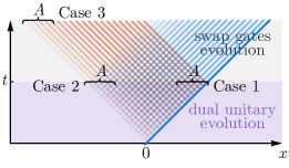
We consider three different cases with different choices for subregion to study the operator entanglement entropy, after evolving by the dual unitary circuit for time , as shown in Fig. 8:
-
1.
contains consecutive sites from the right light-cone edge.
-
2.
contains consecutive sites from the left light-cone edge.
-
3.
contains consecutive left movers from the left light-cone edge.
It worth mention that the Case 3 can be viewed as the operator entanglement on the left light-cone after further evolving the operator by a brick-wall circuit of swap gates (i.e. quenching dual unitary gates to swap gates after time ), such that the left- and right-movers are separated. We will be most interested in the scaling of operator entanglement entropy with the region size in the long-time limit , as the operator has been sufficiently scrambled by the dual unitary circuit to exhibit equilibrium behavior.
III.2.1 Case 1: from the right light-cone edge
We begin with the Case 1, which allows for a direct mean-field description. With the mean-field approximation Eq. (19), we can estimate the th Rényi operator entanglement Eq. (15) as
| (31) |
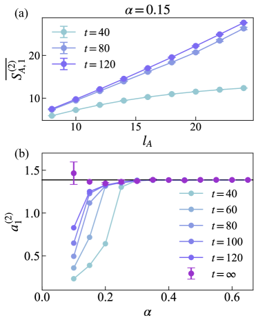
Near the right light-cone, the steady-state operator density, given by Eq. (25), approaches within a length scale of . Therefore, to extract the volume law coefficient of operator entanglement, defined as
we can safely approximate . This leads to the expression , yielding
| (32) |
Since the local operator space has a dimension of 4, this result demonstrates that operator entanglement near the right light-cone is nearly maximal. We demonstrate the maximum growth of the operator entanglement entropy at , i.e., second Rényi entropy in Fig. 9. As one can see in Fig. 9 (a), linear scaling of against the entanglement region (volume law) is observed only after a long enough evolution time , especially at small values. The fitted volume law coefficients against at different are presented in Fig. 9 (b). At large , is found to be maximum , even at small . However, drifts drastically against at small . Therefore, we extrapolate the limit from finite- values, denoted as the purple dots with error bars in Fig. 9 (b). The extrapolated values demonstrate a maximum growth of the operator entanglement entropy for all at , consistent with the mean-field analysis above.
III.2.2 Case 2: from the left light-cone edge
Now, let us consider Case 2 near the left light-cone. Similar to the calculation of the operator density, we introduce the conditional joint distribution function given an emission of a left-mover for the first time at and express the reduced density matrix as follows:
| (33) |
Here, matches the joint distribution with the initial operator , with shifted space-time indices. An important observation is that determines the position of the leftmost particle. Therefore, for and , we have . On the other hand, for , the subsystem contains only the identity operator . Consequently, we can rewrite the reduced density matrix as
| (34) | ||||
Here, all different terms are orthogonal. Taking the mean-field approximation for the conditional distribution, we can express the operator entanglement entropy as
| (35) | ||||
In this equation, we have identified the contribution from as the operator entanglement of a subsystem , which contains sites near the left light-cone for the initial operator . The corresponding result matches the findings of Case 1 for .
To extract the volume-law coefficient, we use . Moreover, for large , we can neglect the last term in Eq. (35). The result reads
| (36) |
Instead of a direct calculation of the summation, we can estimate by extracting the dependence, which scales as with . When we have , the dominant contribution is from , while for , the dominant contribution comes from . Therefore, we have
| (37) |
This suggests a possible transition in operator entanglement as we tune . Unfortunately, since the mapping from the original quantum circuits to the Markovian process requires , the transition point is never accessible for integers . On the other hand, taking the limit leads to . A non-trivial entanglement transition at finite only exist for .
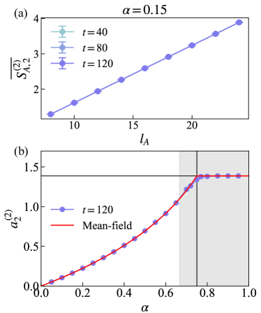
From Eq. (37), the transition for the second Rényi entanglement, appears at . Although is out of the legitimate domain of the dual unitary gate parameter, we can nonetheless perform Monte Carlo sampling in the entire range . Fig. 10 (a) demonstrates the volume law growth of the entanglement entropy. In this case, entanglement entropy converges very quickly against the evolution time such that the data measured at is almost identical to that measured at , in contrast to the strong time-dependent feature observed in Case 1. A transition at is successfully detected by the volume law coefficient : below , increases as consistent with mean-field analysis and remains the maximum value when .
III.2.3 Case 3: from the left light-cone edge, focusing on left-movers only
We can construct a scenario where an entanglement transition can be observed at a finite within the physical range of the gate parameter. This is described in Case 3, where we consider only the subsystem of left movers. Following the analysis of Case 2, the only difference is a reduction of by a factor of two. Therefore, we expect
| (38) |
This results in a change in the critical :
| (39) |
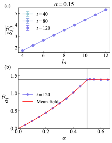
An entanglement transition exists for . In particular, we find for the second Rényi operator entanglement, which is also verified via numerical simulation in Fig. 11 (b). The growing behavior of at the sub-maximal growth region, i.e., , also agrees with the mean-field prediction, which reads at .
III.2.4 Summary of results on operator entanglement
In this subsection, we studied the dynamics of operator entanglement in dual-unitary circuits, examining three distinct cases based on different subregions near the light-cone with the initial operator , as illustrated in Fig. 8. Across all three cases, the th-Rényi operator entanglement entropy , as defined in Eq. (13), exhibits a volume-law scaling on both edges of the light cone in the long-time limit , i.e.
| (40) |
growing linearly with the subregion size . However, the dependence of the volume-law coefficient on the gate parameter and the Rényi index differs between the cases, as summarized in Fig. 12.
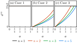
The transition from maximal to sub-maximal volume-law growth in operator entanglement is observed specifically in Case 3, when focusing on the left movers in the left light-cone entanglement region. This result highlights how the gate parameter influence the degree of operator entanglement among the leading left movers emitted from the expanding operator. Such operator entanglement transitions, characterized by the abrupt drop in the volume-law coefficient at a critical value of , have been previously discussed in the literature [39, 36, 35]. Notably, Ref. [36] first identified the operator entanglement transition in a setup akin to our Case 2 and derived the following formula for qubit systems:
| (41) |
where is the leading non-trivial eigenvalue of a transfer matrix defined therein. However, the explicit dependence of on the gate parameter was not fully established. Our study builds upon this foundation by demonstrating that this behavior actually aligns precisely with our Case 3 scenario when we identify .
As a result, we clarify the appropriate entanglement region setup necessary to observe the operator entanglement transition in dual-unitary circuits, providing a mean-field formula for the volume-law coefficient directly in terms of the gate parameter. This result is supported by Monte Carlo simulations, which show excellent agreement with our theoretical predictions.
IV Discussion
In this manuscript, we systematically investigate the operator density evolution and entanglement entropy scaling in dual-unitary circuits by mapping the dynamics to a classical Markov process, enabling efficient Monte Carlo simulations. For operator density, we demonstrate that near the center of the light cone, the operator density converges exponentially to a steady value of , with a rate governed by the gate parameter . In the long-time limit, we derive analytical expressions for the operator density profile’s upper and lower bounds, which are verified through simulations.
For operator entanglement, we analyze three distinct subregions near the light cone and find that the operator entanglement entropy consistently follows a volume-law scaling. However, the volume-law coefficient’s dependence on differs across cases. Notably, we identify a transition from maximal to sub-maximal volume-law growth when focusing on left movers near the left light cone. This transition, characterized by a sudden drop in the volume-law coefficient at a critical , aligns with prior theoretical predictions in the literature [39, 36, 35]. Additionally, we extend this understanding by providing a direct mapping of the volume-law coefficient to the gate parameter, supported by mean-field theory and validated through Monte Carlo simulations. Our work not only clarifies the conditions under which operator entanglement transitions occur but also offers a comprehensive framework for studying operator dynamics and entanglement in dual-unitary circuits.
Our result could have implications in classical shadow tomography [55] and can be extended to random quantum circuits with symmetries. Classical shadow tomography is a recently developed method for efficiently predicting many properties of quantum systems using a limited number of measurements [56, 57, 55, 58]. By understanding operator dynamics and entanglement growth, we can improve the efficiency of classical shadow protocols, leading to more accurate reconstructions of quantum states and observables in many-body systems [59, 60, 61, 62, 63, 64, 65, 66, 67, 68, 69, 70, 71, 72, 73, 74, 75, 76, 77, 78, 79, 80, 81, 82, 83, 84, 85]. More specifically, the advantage of using dual unitary circuit in classical shadow tomography has been recently discussed in Ref. [40].
An interesting future direction is to extend our stochastic simulation framework to random quantum circuits with symmetries, which play a crucial role in modeling realistic quantum systems that conserve quantities such as particle number or spin [5, 86, 87, 88, 89, 90, 91]. Incorporating symmetries into operator dynamics affects the spreading and entanglement properties, offering deeper insights into the role of conserved quantities in quantum information scrambling and thermalization. Our approach provides a pathway to study these effects efficiently, bridging the gap between solvable models and more complex, realistic systems.
Acknowledgements.
Acknowledgments — We thank Yimu Bao, Tian-Gang Zhou for discussions. MHS, TTW and ZYM acknowledge the support from the Research Grants Council (RGC) of Hong Kong (Project Nos. 17301721, AoE/P-701/20, 17309822, HKU C7037-22GF, 17302223, 17301924), the ANR/RGC Joint Research Scheme sponsored by RGC of Hong Kong and French National Research Agency (Project No. A_HKU703/22), the GD-NSF (No. 2022A1515011007). PZ acknowledges the support from the National Natural Science Foundation of China under Grant No. 12374477. YZY is supported by a startup fund from UCSD. We thank HPC2021 system under the Information Technology Services, The University of Hong Kong, as well as the Beijing PARATERA Tech CO.,Ltd. (URL: https://cloud.paratera.com) for providing HPC resources that have contributed to the research results reported within this paper. ZYZ, YZY and ZYM acknowledge the hospitality of Kavli Institute for Theoretical Physics (KITP) and thank the organizers of the KITP program “Correlated Gapless Quantum Matter” where this work was initiated. This research was supported in part by grant NSF PHY-2309135 to the KITP.References
- Ho and Abanin [2017] W. W. Ho and D. A. Abanin, Entanglement dynamics in quantum many-body systems, Phys. Rev. B 95, 094302 (2017).
- Nahum et al. [2017] A. Nahum, J. Ruhman, S. Vijay, and J. Haah, Quantum Entanglement Growth under Random Unitary Dynamics, Physical Review X 7, 031016 (2017).
- Nahum et al. [2018] A. Nahum, S. Vijay, and J. Haah, Operator Spreading in Random Unitary Circuits, Physical Review X 8, 021014 (2018).
- von Keyserlingk et al. [2018] C. W. von Keyserlingk, T. Rakovszky, F. Pollmann, and S. L. Sondhi, Operator Hydrodynamics, OTOCs, and Entanglement Growth in Systems without Conservation Laws, Physical Review X 8, 021013 (2018).
- Khemani et al. [2018] V. Khemani, A. Vishwanath, and D. A. Huse, Operator Spreading and the Emergence of Dissipative Hydrodynamics under Unitary Evolution with Conservation Laws, Physical Review X 8, 031057 (2018).
- Chan et al. [2018] A. Chan, A. De Luca, and J. T. Chalker, Solution of a Minimal Model for Many-Body Quantum Chaos, Physical Review X 8, 041019 (2018).
- Zhou and Chen [2019] T. Zhou and X. Chen, Operator dynamics in a Brownian quantum circuit, Phys. Rev. E 99, 052212 (2019).
- Qi et al. [2019] X.-L. Qi, E. J. Davis, A. Periwal, and M. Schleier-Smith, Measuring operator size growth in quantum quench experiments, arXiv e-prints , arXiv:1906.00524 (2019).
- von Keyserlingk et al. [2022] C. von Keyserlingk, F. Pollmann, and T. Rakovszky, Operator backflow and the classical simulation of quantum transport, Phys. Rev. B 105, 245101 (2022).
- Schuster and Yao [2022] T. Schuster and N. Y. Yao, Operator Growth in Open Quantum Systems, arXiv e-prints , arXiv:2208.12272 (2022).
- Bohrdt et al. [2017] A. Bohrdt, C. B. Mendl, M. Endres, and M. Knap, Scrambling and thermalization in a diffusive quantum many-body system, New Journal of Physics 19, 063001 (2017).
- Kukuljan et al. [2017] I. Kukuljan, S. Grozdanov, and T. Prosen, Weak quantum chaos, Phys. Rev. B 96, 060301 (2017).
- Xu and Swingle [2019] S. Xu and B. Swingle, Locality, Quantum Fluctuations, and Scrambling, Physical Review X 9, 031048 (2019).
- Parker et al. [2019] D. E. Parker, X. Cao, A. Avdoshkin, T. Scaffidi, and E. Altman, A Universal Operator Growth Hypothesis, Physical Review X 9, 041017 (2019).
- Kuo et al. [2020] W.-T. Kuo, A. A. Akhtar, D. P. Arovas, and Y.-Z. You, Markovian entanglement dynamics under locally scrambled quantum evolution, Phys. Rev. B 101, 224202 (2020).
- Akhtar and You [2020] A. A. Akhtar and Y.-Z. You, Multiregion entanglement in locally scrambled quantum dynamics, Phys. Rev. B 102, 134203 (2020).
- Zhang and Zhai [2023] R. Zhang and H. Zhai, Universal Hypothesis of Autocorrelation Function from Krylov Complexity, arXiv e-prints , arXiv:2305.02356 (2023).
- Liu et al. [2023a] C. Liu, H. Tang, and H. Zhai, Krylov complexity in open quantum systems, Physical Review Research 5, 033085 (2023a).
- Buča [2023] B. Buča, Unified Theory of Local Quantum Many-Body Dynamics: Eigenoperator Thermalization Theorems, Physical Review X 13, 031013 (2023).
- Zhang and Gu [2023] P. Zhang and Y. Gu, Operator size distribution in large N quantum mechanics of Majorana fermions, JHEP (10) 018.
- Zhang and Yu [2023] P. Zhang and Z. Yu, Dynamical Transition of Operator Size Growth in Quantum Systems Embedded in an Environment, Phys. Rev. Lett. 130, 250401 (2023).
- Gottesman [1998] D. Gottesman, The Heisenberg Representation of Quantum Computers, arXiv e-prints , quant-ph/9807006 (1998).
- Vidal [2004] G. Vidal, Efficient Simulation of One-Dimensional Quantum Many-Body Systems, Phys. Rev. Lett. 93, 040502 (2004).
- Haegeman et al. [2011] J. Haegeman, J. I. Cirac, T. J. Osborne, I. Pižorn, H. Verschelde, and F. Verstraete, Time-Dependent Variational Principle for Quantum Lattices, Phys. Rev. Lett. 107, 070601 (2011).
- Haegeman et al. [2016] J. Haegeman, C. Lubich, I. Oseledets, B. Vandereycken, and F. Verstraete, Unifying time evolution and optimization with matrix product states, Phys. Rev. B 94, 165116 (2016).
- Muth et al. [2011] D. Muth, R. G. Unanyan, and M. Fleischhauer, Dynamical Simulation of Integrable and Nonintegrable Models in the Heisenberg Picture, Phys. Rev. Lett. 106, 077202 (2011).
- Alba et al. [2019] V. Alba, J. Dubail, and M. Medenjak, Operator Entanglement in Interacting Integrable Quantum Systems: The Case of the Rule 54 Chain, Phys. Rev. Lett. 122, 250603 (2019).
- Jonay et al. [2018] C. Jonay, D. A. Huse, and A. Nahum, Coarse-grained dynamics of operator and state entanglement, arXiv e-prints , arXiv:1803.00089 (2018).
- Zhou and Nahum [2019] T. Zhou and A. Nahum, Emergent statistical mechanics of entanglement in random unitary circuits, Phys. Rev. B 99, 174205 (2019).
- de Groot et al. [2022] C. de Groot, A. Turzillo, and N. Schuch, Symmetry Protected Topological Order in Open Quantum Systems, Quantum 6, 856 (2022).
- Ma and Wang [2023] R. Ma and C. Wang, Average Symmetry-Protected Topological Phases, Physical Review X 13, 031016 (2023).
- Nahum et al. [2022] A. Nahum, S. Roy, S. Vijay, and T. Zhou, Real-time correlators in chaotic quantum many-body systems, Phys. Rev. B 106, 224310 (2022).
- Nie et al. [2019] L. Nie, M. Nozaki, S. Ryu, and M. Tian Tan, Signature of quantum chaos in operator entanglement in 2d CFTs, Journal of Statistical Mechanics: Theory and Experiment 9, 093107 (2019).
- Kudler-Flam et al. [2020] J. Kudler-Flam, M. Nozaki, S. Ryu, and M. T. Tan, Quantum vs. classical information: operator negativity as a probe of scrambling, Journal of High Energy Physics 2020, 31 (2020).
- Bertini et al. [2020a] B. Bertini, P. Kos, and T. Prosen, Operator Entanglement in Local Quantum Circuits II: Solitons in Chains of Qubits, SciPost Phys. 8, 068 (2020a).
- Bertini et al. [2020b] B. Bertini, P. Kos, and T. Prosen, Operator Entanglement in Local Quantum Circuits I: Chaotic Dual-Unitary Circuits, SciPost Phys. 8, 067 (2020b).
- Jamiołkowski [1972] A. Jamiołkowski, Linear transformations which preserve trace and positive semidefiniteness of operators, Reports on Mathematical Physics 3, 275 (1972).
- Choi [1975] M.-D. Choi, Completely positive linear maps on complex matrices, Linear Algebra and its Applications 10, 285 (1975).
- Bertini et al. [2019] B. Bertini, P. Kos, and T. c. v. Prosen, Exact Correlation Functions for Dual-Unitary Lattice Models in Dimensions, Phys. Rev. Lett. 123, 210601 (2019).
- Akhtar et al. [2024a] A. A. Akhtar, N. Anand, J. Marshall, and Y.-Z. You, Dual-Unitary Classical Shadow Tomography, arXiv e-prints , arXiv:2404.01068 (2024a).
- Hamma et al. [2012] A. Hamma, S. Santra, and P. Zanardi, Quantum Entanglement in Random Physical States, Phys. Rev. Lett. 109, 040502 (2012).
- Hayden et al. [2016] P. Hayden, S. Nezami, X.-L. Qi, N. Thomas, M. Walter, and Z. Yang, Holographic duality from random tensor networks, Journal of High Energy Physics 2016, 9 (2016).
- Da Liao [2023] Y. Da Liao, Controllable Incremental Algorithm for Entanglement Entropy in Quantum Monte Carlo Simulations, arXiv e-prints , arXiv:2307.10602 (2023).
- Zhang et al. [2024] X. Zhang, G. Pan, B.-B. Chen, K. Sun, and Z. Y. Meng, Integral algorithm of exponential observables for interacting fermions in quantum Monte Carlo simulations, Phys. Rev. B 109, 205147 (2024).
- Zhou et al. [2024] X. Zhou, Z. Y. Meng, Y. Qi, and Y. Da Liao, Incremental SWAP operator for entanglement entropy: Application for exponential observables in quantum Monte Carlo simulation, Phys. Rev. B 109, 165106 (2024).
- Hastings et al. [2010] M. B. Hastings, I. González, A. B. Kallin, and R. G. Melko, Measuring Renyi Entanglement Entropy in Quantum Monte Carlo Simulations, Phys. Rev. Lett. 104, 157201 (2010).
- Luitz et al. [2014] D. J. Luitz, X. Plat, N. Laflorencie, and F. Alet, Improving entanglement and thermodynamic Rényi entropy measurements in quantum Monte Carlo, Phys. Rev. B 90, 125105 (2014).
- Song et al. [2024a] M. Song, T.-T. Wang, and Z. Y. Meng, Resummation-based quantum Monte Carlo for entanglement entropy computation, Phys. Rev. B 110, 115117 (2024a).
- D’Emidio [2020] J. D’Emidio, Entanglement Entropy from Nonequilibrium Work, Phys. Rev. Lett. 124, 110602 (2020).
- Zhao et al. [2022a] J. Zhao, Y.-C. Wang, Z. Yan, M. Cheng, and Z. Y. Meng, Scaling of Entanglement Entropy at Deconfined Quantum Criticality, Phys. Rev. Lett. 128, 010601 (2022a).
- Zhao et al. [2022b] J. Zhao, B.-B. Chen, Y.-C. Wang, Z. Yan, M. Cheng, and Z. Y. Meng, Measuring Rényi entanglement entropy with high efficiency and precision in quantum Monte Carlo simulations, npj Quantum Materials 7, 69 (2022b).
- Song et al. [2024b] M. Song, J. Zhao, Z. Y. Meng, C. Xu, and M. Cheng, Extracting subleading corrections in entanglement entropy at quantum phase transitions, SciPost Phys. 17, 010 (2024b).
- Wang et al. [2024] T.-T. Wang, M. Song, Z. Y. Meng, and T. Grover, An analog of topological entanglement entropy for mixed states, arXiv e-prints , arXiv:2407.20500 (2024).
- Ippoliti et al. [2023] M. Ippoliti, Y. Li, T. Rakovszky, and V. Khemani, Operator Relaxation and the Optimal Depth of Classical Shadows, Phys. Rev. Lett. 130, 230403 (2023).
- Huang et al. [2020] H.-Y. Huang, R. Kueng, and J. Preskill, Predicting many properties of a quantum system from very few measurements, Nature Physics 16, 1050 (2020).
- Ohliger et al. [2013] M. Ohliger, V. Nesme, and J. Eisert, Efficient and feasible state tomography of quantum many-body systems, New Journal of Physics 15, 015024 (2013).
- Guta et al. [2020] M. Guta, J. Kahn, R. Kueng, and J. A. Tropp, Fast state tomography with optimal error bounds, Journal of Physics A: Mathematical and Theoretical 53, 204001 (2020).
- Elben et al. [2020] A. Elben, R. Kueng, H.-Y. R. Huang, R. van Bijnen, C. Kokail, M. Dalmonte, P. Calabrese, B. Kraus, J. Preskill, P. Zoller, and B. Vermersch, Mixed-State Entanglement from Local Randomized Measurements, Phys. Rev. Lett. 125, 200501 (2020).
- Huang et al. [2021a] H.-Y. Huang, M. Broughton, M. Mohseni, R. Babbush, S. Boixo, H. Neven, and J. R. McClean, Power of data in quantum machine learning, Nature Communications 12, 2631 (2021a).
- Huang et al. [2021b] H.-Y. Huang, R. Kueng, and J. Preskill, Information-Theoretic Bounds on Quantum Advantage in Machine Learning, Phys. Rev. Lett. 126, 190505 (2021b).
- Huang et al. [2021c] H.-Y. Huang, R. Kueng, G. Torlai, V. V. Albert, and J. Preskill, Provably efficient machine learning for quantum many-body problems, arXiv e-prints , arXiv:2106.12627 (2021c).
- Huang et al. [2021d] H.-Y. Huang, R. Kueng, and J. Preskill, Efficient Estimation of Pauli Observables by Derandomization, Phys. Rev. Lett. 127, 030503 (2021d).
- Levy et al. [2021] R. Levy, D. Luo, and B. K. Clark, Classical Shadows for Quantum Process Tomography on Near-term Quantum Computers, arXiv e-prints , arXiv:2110.02965 (2021).
- Acharya et al. [2021] A. Acharya, S. Saha, and A. M. Sengupta, Shadow tomography based on informationally complete positive operator-valued measure, Phys. Rev. A 104, 052418 (2021).
- Hu and You [2022] H.-Y. Hu and Y.-Z. You, Hamiltonian-driven shadow tomography of quantum states, Physical Review Research 4, 013054 (2022).
- Bu et al. [2022] K. Bu, D. Enshan Koh, R. J. Garcia, and A. Jaffe, Classical shadows with Pauli-invariant unitary ensembles, arXiv e-prints , arXiv:2202.03272 (2022).
- Seif et al. [2022] A. Seif, Z.-P. Cian, S. Zhou, S. Chen, and L. Jiang, Shadow Distillation: Quantum Error Mitigation with Classical Shadows for Near-Term Quantum Processors, arXiv e-prints , arXiv:2203.07309 (2022).
- Hu et al. [2022] H.-Y. Hu, R. LaRose, Y.-Z. You, E. Rieffel, and Z. Wang, Logical shadow tomography: Efficient estimation of error-mitigated observables, arXiv e-prints , arXiv:2203.07263 (2022).
- Chau Nguyen et al. [2022] H. Chau Nguyen, J. Lennart Bönsel, J. Steinberg, and O. Gühne, Optimising shadow tomography with generalised measurements, arXiv e-prints , arXiv:2205.08990 (2022).
- Hadfield et al. [2022] C. Hadfield, S. Bravyi, R. Raymond, and A. Mezzacapo, Measurements of Quantum Hamiltonians with Locally-Biased Classical Shadows, Communications in Mathematical Physics 391, arXiv:2006.15788 (2022).
- Huang et al. [2022] H.-Y. Huang, M. Broughton, J. Cotler, S. Chen, J. Li, M. Mohseni, H. Neven, R. Babbush, R. Kueng, J. Preskill, and J. R. McClean, Quantum advantage in learning from experiments, Science 376, 1182 (2022).
- Enshan Koh and Grewal [2022] D. Enshan Koh and S. Grewal, Classical Shadows With Noise, Quantum 6, arXiv:2011.11580 (2022).
- Hao Low [2022] G. Hao Low, Classical shadows of fermions with particle number symmetry, arXiv e-prints , arXiv:2208.08964 (2022).
- Bertoni et al. [2022] C. Bertoni, J. Haferkamp, M. Hinsche, M. Ioannou, J. Eisert, and H. Pashayan, Shallow shadows: Expectation estimation using low-depth random Clifford circuits, arXiv e-prints , arXiv:2209.12924 (2022).
- Arienzo et al. [2022] M. Arienzo, M. Heinrich, I. Roth, and M. Kliesch, Closed-form analytic expressions for shadow estimation with brickwork circuits, arXiv e-prints , arXiv:2211.09835 (2022).
- Hu et al. [2023] H.-Y. Hu, S. Choi, and Y.-Z. You, Classical Shadow Tomography with Locally Scrambled Quantum Dynamics, Physical Review Research 5, arXiv:2107.04817 (2023).
- Akhtar et al. [2023] A. A. Akhtar, H.-Y. Hu, and Y.-Z. You, Scalable and Flexible Classical Shadow Tomography with Tensor Networks, Quantum 7, 1026 (2023).
- Zhang et al. [2024] S. Zhang, X. Feng, M. Ippoliti, and Y.-Z. You, Holographic Classical Shadow Tomography, arXiv e-prints , arXiv:2406.11788 (2024).
- Akhtar et al. [2024b] A. A. Akhtar, H.-Y. Hu, and Y.-Z. You, Measurement-induced criticality is tomographically optimal, Phys. Rev. B 109, 094209 (2024b).
- Hu et al. [2024] H.-Y. Hu, A. Gu, S. Majumder, H. Ren, Y. Zhang, D. S. Wang, Y.-Z. You, Z. Minev, S. F. Yelin, and A. Seif, Demonstration of Robust and Efficient Quantum Property Learning with Shallow Shadows, arXiv e-prints , arXiv:2402.17911 (2024).
- Liu et al. [2023b] Z. Liu, Z. Hao, and H.-Y. Hu, Predicting Arbitrary State Properties from Single Hamiltonian Quench Dynamics, arXiv e-prints , arXiv:2311.00695 (2023b).
- Shen et al. [2024] Y. Shen, A. Buzali, H.-Y. Hu, K. Klymko, D. Camps, S. F. Yelin, and R. Van Beeumen, Efficient Measurement-Driven Eigenenergy Estimation with Classical Shadows, arXiv e-prints , arXiv:2409.13691 (2024).
- Ippoliti and Khemani [2024] M. Ippoliti and V. Khemani, Learnability Transitions in Monitored Quantum Dynamics via Eavesdropper’s Classical Shadows, PRX Quantum 5, 020304 (2024).
- Ippoliti [2024] M. Ippoliti, Classical shadows based on locally-entangled measurements, Quantum 8, 1293 (2024).
- Chen et al. [2024] S. Chen, W. Gong, and Q. Ye, Optimal tradeoffs for estimating Pauli observables, arXiv e-prints , arXiv:2404.19105 (2024).
- Rakovszky et al. [2018] T. Rakovszky, F. Pollmann, and C. W. von Keyserlingk, Diffusive Hydrodynamics of Out-of-Time-Ordered Correlators with Charge Conservation, Physical Review X 8, 031058 (2018).
- Hunter-Jones [2018] N. Hunter-Jones, Operator growth in random quantum circuits with symmetry, arXiv e-prints , arXiv:1812.08219 (2018).
- Agrawal et al. [2022] U. Agrawal, A. Zabalo, K. Chen, J. H. Wilson, A. C. Potter, J. H. Pixley, S. Gopalakrishnan, and R. Vasseur, Entanglement and Charge-Sharpening Transitions in U(1) Symmetric Monitored Quantum Circuits, Phys. Rev. X 12, 041002 (2022).
- Foligno et al. [2024] A. Foligno, P. Calabrese, and B. Bertini, Non-equilibrium dynamics of charged dual-unitary circuits, arXiv e-prints , arXiv:2407.21786 (2024).
- Chang et al. [2024] R.-A. Chang, H. Shrotriya, W. W. Ho, and M. Ippoliti, Deep thermalization under charge-conserving quantum dynamics, arXiv e-prints , arXiv:2408.15325 (2024).
- Fisher et al. [2023] M. P. A. Fisher, V. Khemani, A. Nahum, and S. Vijay, Random Quantum Circuits, Annual Review of Condensed Matter Physics 14, 335 (2023).
