Monopole Fluctuations in Galaxy Surveys

Abstract

Galaxy clustering provides a powerful way to probe cosmology. This requires understanding of the background mean density of galaxy samples, which is estimated from the survey itself by averaging the observed galaxy number density over the angular position. The angle average includes not only the background mean density, but also the monopole fluctuation at each redshift. Here for the first time we compute the monopole fluctuations in galaxy surveys and investigate their impact on galaxy clustering. The monopole fluctuations vary as a function of redshift, and it is correlated with other fluctuations, affecting the two-point correlation function measurements. In an idealized all-sky survey, the rms fluctuation at $z=0.5$ can be as large as 7% of the two-point correlation function in amplitude at the BAO scale, and it becomes smaller than 1% at $z>2$. The monopole fluctuations are unavoidable, but they can be modeled. We discuss its relation to the integral constraint and the implications for the galaxy clustering analysis.

Introduction.— The expansion history of the Universe is one of the key ingredients for understanding the energy contents of the Universe, and one of the best ways to achieve this goal is to measure the distance-redshift relation of cosmological probes such as the cosmic microwave background (CMB) temperature anisotropies and galaxy clustering. The baryonic acoustic oscillation (BAO) signal, which arises from the coupling of baryons and photons in the early Universe Peebles and Yu (1970); Sunyaev and Zeldovich (1970), is a standard ruler that can be used to measure the angular diameter distances to the last scattering surface and to the galaxy surveys. In particular, with the discovery of the late-time cosmic acceleration Riess et al. (1998); Perlmutter et al. (1999), precise measurements of the expansion history in the late Universe are one of the primary goals in the recent and upcoming large-scale galaxy surveys York et al. (2000); Colless et al. (2001); Eisenstein et al. (2011); Levi et al. (2013); Stubbs et al. (2004); Laureijs et al. (2011); Green et al. (2012), and the BAO signals in galaxy clustering have been detected with ever increasing precision Eisenstein et al. (2005); Blake et al. (2007); Percival et al. (2010); Anderson et al. (2012); Ata et al. (2018); Bautista et al. (2021); DESI Collaboration et al. (2024a) (see Eisenstein and Hu (1998); Eisenstein et al. (2007); Weinberg et al. (2013) for recent reviews).

For analyzing galaxy clustering, the background mean number density of the galaxy samples should be subtracted, before the BAO signals can be measured. Without full understanding of complex process of galaxy formation and evolution, the mean number density is estimated from the survey itself, which is then modulated by fluctuations of wavelength larger than the survey volume. The survey volume at each redshift is limited by a full-sky coverage, and the fluctuation over the entire sky is called the monopole fluctuation, indistinguishable from the background mean value. In this Letter, for the first time we compute the monopole fluctuations in galaxy surveys and study the impact of the monopole fluctuations on the two-point correlation function at the BAO scales.

Observed Mean and the Integral Constraint.— Here we briefly describe the standard procedure to estimate the observed mean number density and analyze the galaxy number density fluctuation, which is subject to the integral constraint Peebles (1980); Peacock and Nicholson (1991). The observed galaxy number density at the observed redshift $z$ and angle $\hat{\bm{n}}$ can be written as

$$n_{g}^{\rm obs}(z,\hat{\bm{n}})=\bar{n}_{g}(z)\Big{[}1+\delta_{g}(z,\hat{\bm{n}})\Big{]}~{},$$ (1)

where $\bar{n}_{g}(z)$ is the number density in a background universe and $\delta_{g}(z,\hat{\bm{n}})$ is the fluctuation of the observed galaxy number density. The galaxy number density fluctuation $\delta_{g}$ at the observed redshift is mainly driven by the matter density fluctuation Kaiser (1984); Bardeen et al. (1986) and the redshift-space distortion Kaiser (1987), in addition to the gravitational lensing effect Narayan (1989) and other relativistic effects Sachs and Wolfe (1967). The full relativistic expression for $\delta_{g}$ has been derived and shown to be gauge-invariant Yoo et al. (2009); Yoo (2010); Bonvin and Durrer (2011). The goal is to compare various statistics of the galaxy number density fluctuation $\delta_{g}$ to the measurements in galaxy surveys. However, we do not know a priori the background number density $\bar{n}_{g}(z)$, and hence we cannot directly measure $\delta_{g}$. This is in contrast to the cases Yoo et al. (2019a, b); Baumgartner and Yoo (2021) for the CMB temperature anisotropies or the matter density fluctuations, in which we know their background redshift evolution $\bar{T}\propto(1+z)$ or $\bar{\rho}_{m}\propto(1+z)^{3}$ and their values today ($\Omega_{\gamma}$ and $\Omega_{m}$) are part of a cosmological model with the adopted values for all the cosmological parameters (including $\Omega_{\gamma}$ and $\Omega_{m}$).

Without a priori knowledge on the background number density and its redshift evolution, the observers use the survey data to measure the observed mean $\bar{n}_{g,\Omega}^{\rm obs}(z)$ by simply averaging the observed galaxy number density $n_{g}^{\rm obs}(z,\hat{\bm{n}})$ over the observed angle $\hat{\bm{n}}$ as a function of redshift $z$ (see, e.g., Eisenstein et al. (2001); Cool et al. (2008); White et al. (2011); DESI Collaboration et al. (2024a)):

$$\bar{n}_{g,\Omega}^{\rm obs}(z):=\int{d^{2}\hat{n}\over 4\pi}~{}n_{g}^{\rm obs}(z,\hat{\bm{n}})=\bar{n}_{g}(z)\Big{[}1+\delta n(z)\Big{]}~{},$$ (2)

where we defined the dimensionless angle-averaged galaxy fluctuation $\delta n(z)$ (or the monopole fluctuation) as

$$\delta n(z):=\int{d^{2}\hat{n}\over 4\pi}~{}\delta_{g}(z,\hat{\bm{n}})~{}.$$ (3)

Mind that only $\bar{n}_{g,\Omega}^{\rm obs}(z)$ is an observable, not $\bar{n}_{g}(z)$ or $\delta n(z)$ separately. For simplicity, we have assumed an idealized full-sky survey and ignored technical difficulties in practice such as a non-uniform angular selection function throughout the paper.

Hence the observed galaxy number density can be re-arranged in terms of the observed mean as

$$n_{g}^{\rm obs}(z,\hat{\bm{n}})=\bar{n}_{g,\Omega}^{\rm obs}(z)~{}{1+\delta_{g}(z,\hat{\bm{n}})\over 1+\delta n(z)}~{},$$ (4)

and the observed galaxy fluctuation is then

$$\delta_{g}^{\rm obs}(z,\hat{\bm{n}}):={n_{g}^{\rm obs}(z,\hat{\bm{n}})\over\bar{n}_{g,\Omega}^{\rm obs}(z)}-1={\delta_{g}(z,\hat{\bm{n}})-\delta n(z)\over 1+\delta n(z)}~{},$$ (5)

different from the standard theoretical prediction $\delta_{g}(z,\hat{\bm{n}})$. Expanding to the linear order in perturbation, we obtain the expression

$$\delta_{g}^{\rm obs}(z,\hat{\bm{n}})\approx\delta_{g}(z,\hat{\bm{n}})-\delta n(z)~{},$$ (6)

for the observed galaxy fluctuation we will use in this work. Naturally, the observed galaxy fluctuation is subject to the integral constraint at a given redshift:

$$0=\int~{}d^{2}\hat{n}~{}\delta_{g}^{\rm obs}(z,\hat{\bm{n}})~{}~{}~{}~{}~{}{\rm for}~{}\forall~{}z\in{\rm survey}~{},$$ (7)

while the standard galaxy fluctuation $\delta_{g}(z,\hat{\bm{n}})$ is not subject to the same integral constraint:

$$0\neq\int~{}d^{2}\hat{n}~{}\delta_{g}(z,\hat{\bm{n}})~{}.$$ (8)

Note that the standard integral constraint in Peacock and Nicholson (1991) is formulated in terms of average over the survey volume, rather than average over the angle at each redshift. Our equation (7) would correspond to the radial integral constraint in de Mattia and Ruhlmann-Kleider (2019).

Monopole Fluctuations.— Our task now is to compute the monopole fluctuations in Equation (3) as a function of redshift. In the past, little attention was paid to the monopole fluctuations, as gauge issues in the monopole fluctuations result in infrared divergences and the monopole fluctuation cannot be separated from the background mean value Zibin and Scott (2008). First, the presence of infrared divergences in cosmological observables such as the luminosity distance, CMB anisotropies implies the deficiency in the theoretical descriptions, and it was shown Biern and Yoo (2017a, b); Scaccabarozzi et al. (2018); Grimm et al. (2020); Baumgartner and Yoo (2021) that fully relativistic gauge-invariant theoretical descriptions of the cosmological observables resolve the issues. Regarding the latter, can we measure the monopole fluctuations? Yes, they can be measured separately Yoo et al. (2019a); Baumgartner and Yoo (2021), if the background evolution is known (e.g., the matter density, the CMB temperature). Though this is not the case for galaxy clustering, its impact is present in the galaxy $N$-point statistics. Here for the first time we compute the monopole fluctuations in galaxy surveys.

To investigate the monopole fluctuations, we decompose the expression for the galaxy fluctuation $\delta_{g}$ in terms of spherical harmonics $Y_{lm}(\hat{\bm{n}})$ as

$$\delta_{g}(z,\hat{\bm{n}})=\sum_{lm}a_{lm}(z)Y_{lm}(\hat{\bm{n}})~{},$$ (9)

and the angular power spectrum is

$$C_{l}(z_{1},z_{2})=\left\langle a_{lm}(z_{1})a_{lm}^{*}(z_{2})\right\rangle~{}.$$ (10)

The observed galaxy fluctuation $\delta_{g}^{\rm obs}$ can be decomposed in the same way, and its angular multipoles $a_{lm}^{\rm obs}$ are related to the angular multipoles $a_{lm}$ of $\delta_{g}$ in Equation (9) as

$$a_{lm}^{\rm obs}(z)={a_{lm}(z)\over 1+\delta n(z)}\qquad{\rm for}~{}~{}l\geq 1~{}.$$ (11)

Since $\bar{n}_{g,\Omega}^{\rm obs}(z)$ that includes the monopole fluctuation is defined as the observed mean, the observed galaxy fluctuation $\delta_{g}^{\rm obs}$ has no monopole fluctuation:

$$a_{00}^{\rm obs}=0~{},$$ (12)

exactly in the same way the observed CMB temperature from the COBE FIRAS measurements Mather et al. (1994); Fixsen et al. (1996); Fixsen (2009) includes the background temperature and the monopole fluctuation. The monopole fluctuation in Equation (3) is related to $a_{00}$ as

$$\delta n(z)={1\over\sqrt{4\pi}}~{}a_{00}(z)~{}.$$ (13)

Using Equations (9) and (10), the monopole power can be written as

$$C_{0}(z_{1},z_{2})=4\pi\int d\ln k~{}\Delta^{2}_{\cal R}(k)~{}{\cal T}_{0}(k,z_{1}){\cal T}_{0}(k,z_{2})~{},$$ (14)

where $\Delta^{2}_{\cal R}(k)=A_{s}(k/k_{0})^{n_{s}-1}$ is the dimensionless scale-invariant power spectrum of the comoving-gauge curvature perturbation $\cal R$ at the initial time and ${\cal T}_{0}(k,z)$ is the monopole transfer function for the galaxy fluctuation $\delta_{g}$ at redshift $z$. For numerical computation, we assume the standard $\Lambda$CDM model, in which the primordial fluctuation amplitude $A_{s}=2.1\times 10^{-9}$, the spectral index $n_{s}=0.966$, the Hubble parameter $h=0.6732$, consistent with the best-fit parameters from the Planck collaboration Planck Collaboration et al. (2020); Planck Collaboration et al. (2018). To a good approximation, we can compute the monopole transfer function by accounting for the matter density fluctuation $\delta_{m}$ with the galaxy bias factor $b$ and the redshift-space distortion from the line-of-sight velocity $V_{\parallel}$:

$${\cal T}_{0}(k,z)=b~{}{\cal T}_{m}(k,z)j_{0}(k\bar{r}_{z})+{k^{2}\over\mathcal{H}_{z}}{\cal T}_{v_{m}}(k,z)j_{0}^{\prime\prime}(k\bar{r}_{z})~{},$$ (15)

where $j_{0}(x)$ is the spherical Bessel function, $\bar{r}_{z}$ is the comoving distance to the redshift $z$, $\mathcal{H}_{z}$ is the conformal Hubble parameter, ${\cal T}_{m}$ and ${\cal T}_{v_{m}}$ are the transfer functions for the (comoving-gauge) matter density fluctuation and the (Newtonian-gauge) velocity potential ($V_{\parallel}=:-\hat{\bm{n}}\cdot\nabla v_{m}$).

Figure 1: Transfer functions ${\cal T}_{i}(k)$ for the individual perturbations $\delta p_{i}$ defined as $\delta p_{i}({\bf k},z)={\cal T}_{i}(k,z){\cal R}({\bf k})$. Various curves show the transfer functions at redshift $z=0$ for the matter density fluctuation $\delta_{m}$ (solid), the velocity potential $v_{m}$ (dashed), the gravitational potential $\psi$ (dotted), and the time-derivative of the gravitational potential (dot dashed). Mind that ${\cal T}_{m}$ is scaled by $10^{3}$ to fit in the plot. The short vertical line indicates the wavenumber that corresponds to the first peak in $j_{0}(k\bar{r}_{z})$ at redshift $z=1$.

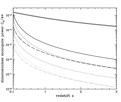
Figure 2: Monopole power $C_{0}(z)/4\pi$ and the impact on the two-point correlation function. Thick solid curve shows the amplitude of the two-point matter density correlation function at the BAO peak position. Black curves (solid, dotted, dashed) show the monopole power $C_{0}(z)/4\pi$ as a function of redshift $z$ from the matter density fluctuation (dotted), the redshift-space distortion (dashed), and their sum (solid). Gray curves (solid, dotted, dashed) show $C_{0}(z_{1},z_{2})/4\pi$ as a function of redshift $z$, with two redshifts $z_{1}$, $z_{2}$ of the galaxy pair, corresponding to the line-of-sight separation $r=100~{}{h^{-1}{\rm Mpc}}$, and with redshift $z$ corresponding to the half the separation.

Figure 1 shows the transfer functions of the individual perturbations in the galaxy fluctuation $\delta_{g}$ at redshift $z$. The transfer functions are defined as $\delta p_{i}({\bf k},z)=:{\cal T}_{i}(k,z){\cal R}({\bf k})$ in terms of the initial fluctuation ${\cal R}$. The matter density fluctuation (solid in Figure 1, the first term in Eq. [15]) is the dominant contribution to galaxy clustering Kaiser (1984), and the other contributions such as the line-of-sight velocity (dashed) and the gravitational potential (dotted) are smaller by orders of magnitude. The vertical line indicates the scale at $z=1$, beyond which the contributions of the individual transfer functions are further suppressed due to the spherical Bessel function $j_{0}(x)$ in the monopole transfer function ${\cal T}_{0}(k,z)$. Note that the transfer function slope for the matter density fluctuation asymptotically reaches $\sim 0.34$ on small scales. On large scales ($x\ll 1$), the transfer functions for the gravitational potential are constant, responsible for infrared divergences in the monopole fluctuations. Their contributions, however, collectively cancel on large scales and remain small, if a correct relativistic formula is used Jeong et al. (2012); Scaccabarozzi et al. (2018); Grimm et al. (2020); Mitsou et al. (2023); Magi and Yoo (2023). Note that there is no gravitational lensing contribution $\kappa$ in the monopole transfer function. The second term in Equation (15) is the redshift-space distortion Kaiser (1987), or the spatial derivative of the line-of-sight velocity, which can be re-arranged as $-f~{}{\cal T}_{m}(k,z)j_{0}^{\prime\prime}(k\bar{r}_{z})$ by using the Einstein equation with the logarithmic growth rate $f$.

The (black) dotted curve in Figure 2 shows the monopole power $C_{0}$ scaled with $4\pi$ from the matter density fluctuation $\delta_{m}$ (or a constant bias factor $b=1$ for the galaxy sample). Given that the initial condition $\Delta^{2}_{\cal R}(k)$ is nearly scale-invariant ($n_{s}\approx 1$), the monopole power in Equation (14) can be read off from the transfer functions in Figure 1 at the peak of the spherical Bessel function. The matter density fluctuation decreases with increasing redshift, as the decreasing growth factor $D(z)$ reduces the overall amplitude of the transfer function. Furthermore, with larger comoving distance $\bar{r}_{z}$, the contributions of the individual transfer functions are shifted to a larger characteristic scale $k\sim 1/\bar{r}_{z}$, further reducing the monopole power at higher redshift. The black dashed curve represents the contribution of the redshift-space distortion. Though modulated differently with $j_{0}^{\prime\prime}(x)$, it closely follows the shape of the matter density power, especially at high redshift, where $f\simeq 1$. Finally, the solid curve shows the full monopole power from the matter density fluctuation and the redshift-space distortion in Equation 15. Note that both contributions oscillate with different periods and the monopole power represents the combined transfer functions at the peak. For our base model ($b=1$), the monopole power $C_{0}/4\pi\approx 10^{-3}$ at $z=0.1$, but decreases rapidly below $10^{-5}$ beyond $z=1$.

Impact on the Two-Point Correlation Function.— Having computed the monopole power as a function of redshift, we are now in a position to quantify the impact of the monopole fluctuations on the two-point correlation function measurements. Given the configuration of two galaxies and the observed galaxy fluctuation in Equation (6), we compute the ensemble average, or the two-point correlation function:

$$\left\langle\delta_{g}^{\rm obs}(\bm{x}_{1})\delta_{g}^{\rm obs}(\bm{x}_{2})\right\rangle=\left\langle\delta_{g}(\bm{x}_{1})\delta_{g}(\bm{x}_{2})\right\rangle-\left\langle\delta n(z_{1})\delta n(z_{2})\right\rangle~{},~{}~{}~{}~{}~{}~{}$$ (16)

where we shortened the notation $\bm{x}=(z,\hat{\bm{n}})$. We can show that three additional terms in the observed two-point correlation function are indeed identical to the angular monopole power $C_{0}(z_{1},z_{2})$:

$$\left\langle\delta n(z_{1})\delta n(z_{2})\right\rangle=\left\langle\delta n(z_{1})\delta_{g}(\bm{x}_{2})\right\rangle={1\over 4\pi}C_{0}(z_{1},z_{2})~{}.$$ (17)

Equation (16) can be better expressed as

$$\xi_{g}^{\rm obs}(r)=\xi_{g}(r)-{1\over 4\pi}~{}C_{0}(z_{1},z_{2})~{},$$ (18)

such that the correlation function $\xi_{g}^{\rm obs}(r)$ we measure in surveys is the correlation function $\xi_{g}(r)$ we predict with $\delta_{g}$ with the monopole power $C_{0}(z_{1},z_{2})/4\pi$ taken out, where $r$ is the separation between two galaxy positions.

Equation (16) is valid, as both hand sides are ensemble averaged. The ensemble averages in practice can be replaced by averaging over many galaxy pairs in the same configurations in surveys. However, the monopole fluctuations that appear in Equation (6) or (16) before ensemble average correspond to a single realization of random fluctuations at each redshift. Nevertheless, we used the ensemble average to compute its contribution to $\xi_{g}^{\rm obs}(r)$. With these caveats, here we use Equation (18) to investigate the impact of the monopole fluctuations on the measurements of the observed two-point correlation function. As shown in Figure 2, the monopole power is $C_{0}(z)/4\pi\simeq 10^{-3}$ at $z=0.1$ and decreasing fast at higher redshift (solid), if galaxies are simply modeled as the matter fluctuation. Hence the impact is negligible, whenever $\xi_{g}\gg 10^{-3}$, which is the case for most of the dynamic range of the correlation function measurements. However, the monopole fluctuations may be relevant on large scales such as the BAO scale, where $\xi_{g}$ is small.

While the monopole power is just a function of two redshifts $z_{1}$ and $z_{2}$ of the observed galaxies, independent of their angular positions, it affects not only the observed correlation function along the line-of-sight direction, but also the observed correlation function along the transverse direction. First, for all the configurations of two galaxies at the same redshift $z$ (or along the transverse direction), the monopole power remains unchanged $C_{0}(z)/4\pi$, regardless of their physical separation $r$ set by two angular directions $\hat{\bm{n}}_{1}$ and $\hat{\bm{n}}_{2}$ at the same redshift $z$. Hence, the correction is a constant shift in the transverse correlation function, but this shift is a function of redshift, as shown in Figure 2 (black curves). Second, for a configuration of two galaxies along the line-of-sight direction (same $\hat{\bm{n}}$, but two different redshifts $z_{1}$ and $z_{2}$), the monopole power $C_{0}(z_{1},z_{2})/4\pi$ in this case is directly a function of their separation $r$, as the difference in the comoving distances $\bar{r}_{z}$ at two redshifts is directly related to the separation $r$.

Gray curves in Figure 2 show the monopole power $C_{0}(z_{1},z_{2})/4\pi$ along the line-of-sight direction for two galaxies located at $z_{1}$ and $z_{2}$, with the corresponding separation $r=100~{}{h^{-1}{\rm Mpc}}$. The dotted and dashed curves represent the matter density fluctuation and the redshift-space distortion, while the solid curve is the combination. With destructive interference of two spherical Bessel functions from two different distances $\bar{r}_{z}$, the monopole power at two different redshifts with $r=100{h^{-1}{\rm Mpc}}$ is negative and smaller in the absolute amplitude than the monopole power at the same redshift.

The thick solid curve in Figure 2 shows the amplitude of the matter density two-point correlation function $\xi_{m}(r)$ at the BAO peak position. As described, the exact correction $C_{0}(z_{1},z_{2})/4\pi$ to be made to $\xi_{g}(r)$ depends on the configuration of two galaxy pairs, but here we make a simple estimate, leaving the detailed investigation for a future work Magnoli et al. (2024). At redshift $z=0.5$, the monopole power affects the amplitude of two-point correlation function at the BAO peak position by 7% along the transverse direction or smaller along the line-of-sight direction. This ratio decreases at higher redshift to 1% at $z=2$ along the transverse direction. In our simple model for galaxies ($b=1$), while the ratio is independent of the growth factor $D(z)$, it decreases at high redshift due to the increase in characteristic scale $k\sim 1/\bar{r}_{z}$ of $C_{0}(z)$. However, we stress that our results are obtained in a full-sky survey.

Conclusion and Discussion.— The galaxy mean number density needs to be subtracted for galaxy clustering analysis, and without ab initio knowledge of galaxy evolution, the mean number density is estimated from the survey itself. Since the observed mean contains the monopole fluctuation at each redshift, the observed galaxy two-point correlation function is affected by the monopole fluctuations. For the same reason, any $N$-point statistics such as the three-point correlation function will be affected by the monopole fluctuations. Since the monopole fluctuation $\delta n\sim\sqrt{C_{0}}$ is small ($C_{0}\approx 10^{-3}$ at $z=0.1$ and $C_{0}\approx 10^{-5}$ at $z=1$), the impact of the monopole fluctuation is, however, limited to large scales such as the BAO scale, where the two-point correlation function is small. Assuming the rms value for the monopole fluctuations, we find that the corrections to the two-point correlation function can be as large as 7% at $z=0.5$ and 1% at $z=2$ in the amplitude at the BAO scale for a survey with full sky coverage.

For simplicity, we have assumed a constant bias factor $b=1$ for the galaxy sample and ignored nonlinearity in the transfer functions. Different values of the galaxy bias factor and its time evolution will certainly change the ratio of the corrections from the monopole fluctuations to the two-point correlation function, albeit not significantly. Despite the suppression from the spherical Bessel function, nonlinearity in the transfer functions can enhance the monopole fluctuations by boosting the transfer function on small scales, in particular at low redshift, where the nonlinearity is significant and the characteristic scale $k\sim 1/\bar{r}_{z}$ approaches the nonlinear scale.

The monopole fluctuations represent the fundamental limitation to our theoretical modeling of the two-point correlation function, or the cosmic variance. They cannot be removed even in idealized surveys with infinite volume, as we only have access to a single light cone volume and there exists only one realization of the monopole fluctuations at each redshift. Without full Euclidean average including translation of the observer position Mitsou et al. (2020), the ensemble average cannot be replaced by spatial average, and any measurements of random fluctuations are inevitably limited by the cosmic variance (see, e.g., Peebles (1980); Peacock (1999); Dodelson (2003)). While the galaxy evolution should be locally smooth and close to a passive evolution $(\bar{n}_{g}\propto 1/a^{3})$ if limited to a small redshift bin $\Delta z$, it would remain difficult to separate, as the monopole fluctuations $\delta n(z)$ are small, i.e., 1% in $\bar{n}_{g}(z)$ at $z=1$.

In practice, the observed mean is often estimated by either the spline fit to the redshift distribution or shuffling the redshift measurements in surveys (see Samushia et al. (2012) for details), which can mitigate some bias arising from galaxy clustering. This clustering would correspond to the corrections from higher angular multipole fluctuations at each redshift, but the monopole fluctuations cannot be removed by shuffling the angular positions. For the same reason, when the sky coverage is incomplete, subsequent angular multipoles such as the dipole fluctuations and so on can act as the monopole fluctuations in the full sky, as those low angular multipole fluctuations at each redshift are again indistinguishable from the mean number density with a partial sky coverage. The “monopole” fluctuation defined in Equation (3) will depend not only on $C_{0}$, but also all $C_{l}$ with $l\geq 0$ in surveys with incomplete sky coverage. Its impact on galaxy clustering will require further numerical studies beyond the scope of current work. Complicated angular selection functions in real surveys such as holes, disjoint patches would also affect the observed mean number density.

The observed correlation function in galaxy surveys is analyzed by further averaging over the angle of the separation vector for a galaxy pair, such as the monopole correlation $\xi_{0}(r)$, the quadrupole $\xi_{2}(r)$, and the hexadecapole $\xi_{4}(r)$ Hamilton (1992); Cole et al. (1994) (see Hawkins et al. (2003); Reid et al. (2012); Beutler et al. (2017) for recent measurements). While the monopole fluctuation $\delta n(z)$ is independent of angular separation, it depends on redshift, such that the effects of the monopole fluctuations on measurements of the multipole correlation functions $\xi_{l}(r)$ are non-trivial and requires further investigations Magnoli et al. (2024). In contrast, the power spectrum analysis is non-local by nature, and the integral constraint is always part of the power spectrum analysis Peacock and Nicholson (1991); Feldman et al. (1994); Vogeley and Szalay (1996); Tegmark et al. (1997). Hence we suspect that the impact on the power spectrum analysis is likely to be small, though there might be tangible impact again on the redshift-space multipole power spectra de Mattia and Ruhlmann-Kleider (2019) due to the integral constraint specified in Equation (7), rather than integration over the volume in the standard power spectrum analysis.

The BAO peak position measured in galaxy surveys is a standard ruler, by which we infer the angular diameter distances to the galaxy samples and constrain cosmological parameters Eisenstein et al. (2005); Blake et al. (2007); Percival et al. (2010); Anderson et al. (2012); Ata et al. (2018); Bautista et al. (2021); DESI Collaboration et al. (2024a). Measurements of the BAO peak position in the correlation function are, however, performed by first marginalizing over the smooth power around the peak position due to the nonlinearity and scale-dependent galaxy bias Seo et al. (2008); DESI Collaboration et al. (2024b). Hence, while the monopole fluctuations are expected to affect the measurements of the BAO peak position especially at low redshift, its precise impact after the marginalization process requires further investigations beyond the scope of this work.

We acknowledge useful discussions with Yan-Chuan Cai. This work is supported by the Swiss National Science Foundation and a Consolidator Grant of the European Research Council.

References

- Peebles and Yu (1970) P. J. E. Peebles and J. T. Yu, Astrophys. J. 162, 815 (1970).
- Sunyaev and Zeldovich (1970) R. A. Sunyaev and Y. B. Zeldovich, Ap&SS 2, 66 (1970).
- Riess et al. (1998) A. G. Riess et al., Astron. J. 116, 1009 (1998), eprint arXiv:astro-ph/9805201.
- Perlmutter et al. (1999) S. Perlmutter et al., Astrophys. J. 517, 565 (1999), eprint arXiv:astro-ph/9812133.
- York et al. (2000) D. G. York et al., Astron. J. 120, 1579 (2000), eprint arXiv:astro-ph/0006396.
- Colless et al. (2001) M. Colless et al., Mon. Not. R. Astron. Soc. 328, 1039 (2001), eprint arXiv:astro-ph/0106498.
- Eisenstein et al. (2011) D. J. Eisenstein, D. H. Weinberg, E. Agol, H. Aihara, C. Allende Prieto, S. F. Anderson, J. A. Arns, É. Aubourg, S. Bailey, E. Balbinot, et al., Astron. J. 142, 72 (2011), eprint 1101.1529.
- Levi et al. (2013) M. Levi, C. Bebek, T. Beers, R. Blum, R. Cahn, D. Eisenstein, B. Flaugher, K. Honscheid, R. Kron, O. Lahav, et al., ArXiv e-prints (2013), eprint 1308.0847.
- Stubbs et al. (2004) C. W. Stubbs, D. Sweeney, J. A. Tyson, and LSST Collaboration, in American Astronomical Society Meeting Abstracts (2004), vol. 36 of Bulletin of the American Astronomical Society, p. 108.02.
- Laureijs et al. (2011) R. Laureijs, J. Amiaux, S. Arduini, J. . Auguères, J. Brinchmann, R. Cole, M. Cropper, C. Dabin, et al., ArXiv e-prints (2011), eprint 1110.3193.
- Green et al. (2012) J. Green, P. Schechter, C. Baltay, R. Bean, D. Bennett, R. Brown, C. Conselice, M. Donahue, et al. (2012), eprint 1208.4012.
- Eisenstein et al. (2005) D. J. Eisenstein, I. Zehavi, D. W. Hogg, R. Scoccimarro, et al., Astrophys. J. 633, 560 (2005), eprint arXiv:astro-ph/0501171.
- Blake et al. (2007) C. Blake, A. Collister, S. Bridle, and O. Lahav, Mon. Not. R. Astron. Soc. 374, 1527 (2007), eprint arXiv:astro-ph/0605303.
- Percival et al. (2010) W. J. Percival, B. A. Reid, D. J. Eisenstein, N. A. Bahcall, T. Budavari, J. A. Frieman, et al., Mon. Not. R. Astron. Soc. 401, 2148 (2010), eprint 0907.1660.
- Anderson et al. (2012) L. Anderson, E. Aubourg, S. Bailey, D. Bizyaev, M. Blanton, A. S. Bolton, J. Brinkmann, J. R. Brownstein, et al., Mon. Not. R. Astron. Soc. 427, 3435 (2012), eprint 1203.6594.
- Ata et al. (2018) M. Ata, F. Baumgarten, J. Bautista, F. Beutler, D. Bizyaev, et al., Mon. Not. R. Astron. Soc. 473, 4773 (2018), eprint 1705.06373.
- Bautista et al. (2021) J. E. Bautista, R. Paviot, M. Vargas Magaña, S. de la Torre, S. Fromenteau, et al., Mon. Not. R. Astron. Soc. 500, 736 (2021), eprint 2007.08993.
- DESI Collaboration et al. (2024a) DESI Collaboration, A. G. Adame, J. Aguilar, S. Ahlen, S. Alam, Alexander, et al., arXiv e-prints arXiv:2404.03002 (2024a), eprint 2404.03002.
- Eisenstein and Hu (1998) D. J. Eisenstein and W. Hu, Astrophys. J. 496, 605 (1998), eprint arXiv:astro-ph/9709112.
- Eisenstein et al. (2007) D. J. Eisenstein, H.-J. Seo, and M. White, Astrophys. J. 664, 660 (2007), eprint arXiv:astro-ph/0604361.
- Weinberg et al. (2013) D. H. Weinberg, M. J. Mortonson, D. J. Eisenstein, C. Hirata, A. G. Riess, and E. Rozo, Phys. Rep. 530, 87 (2013), eprint 1201.2434.
- Peebles (1980) P. J. E. Peebles, The large-scale structure of the universe (Princeton University Press, Princeton, 1980).
- Peacock and Nicholson (1991) J. A. Peacock and D. Nicholson, Mon. Not. R. Astron. Soc. 253, 307 (1991).
- Kaiser (1984) N. Kaiser, Astrophys. J. Lett. 284, L9 (1984).
- Bardeen et al. (1986) J. M. Bardeen, J. R. Bond, N. Kaiser, and A. S. Szalay, Astrophys. J. 304, 15 (1986).
- Kaiser (1987) N. Kaiser, Mon. Not. R. Astron. Soc. 227, 1 (1987).
- Narayan (1989) R. Narayan, Astrophys. J. Lett. 339, L53 (1989).
- Sachs and Wolfe (1967) R. K. Sachs and A. M. Wolfe, Astrophys. J. 147, 73+ (1967).
- Yoo et al. (2009) J. Yoo, A. L. Fitzpatrick, and M. Zaldarriaga, Phys. Rev. D 80, 083514 (2009), eprint arXiv:0907.0707.
- Yoo (2010) J. Yoo, Phys. Rev. D 82, 083508 (2010), eprint arXiv:1009.3021.
- Bonvin and Durrer (2011) C. Bonvin and R. Durrer, Phys. Rev. D 84, 063505 (2011), eprint arXiv:1105.5280.
- Yoo et al. (2019a) J. Yoo, E. Mitsou, Y. Dirian, and R. Durrer, Phys. Rev. D 100, 063510 (2019a), eprint 1905.09288.
- Yoo et al. (2019b) J. Yoo, E. Mitsou, N. Grimm, R. Durrer, and A. Refregier, J. Cosmol. Astropart. Phys. 2019, 015 (2019b), eprint 1905.08262.
- Baumgartner and Yoo (2021) S. Baumgartner and J. Yoo, Phys. Rev. D 103, 063516 (2021), eprint 2012.03968.
- Press and Schechter (1974) W. H. Press and P. Schechter, Astrophys. J. 187, 425 (1974).
- Bond et al. (1991) J. R. Bond, S. Cole, G. Efstathiou, and N. Kaiser, Astrophys. J. 379, 440 (1991).
- Eisenstein et al. (2001) D. J. Eisenstein, J. Annis, J. E. Gunn, A. S. Szalay, A. J. Connolly, R. C. Nichol, N. A. Bahcall, M. Bernardi, S. Burles, F. J. Castander, et al., Astron. J. 122, 2267 (2001), eprint arXiv:astro-ph/0108153.
- Cool et al. (2008) R. J. Cool, D. J. Eisenstein, X. Fan, M. Fukugita, L. Jiang, C. Maraston, A. Meiksin, D. P. Schneider, and D. A. Wake, Astrophys. J. 682, 919 (2008), eprint 0804.4516.
- White et al. (2011) M. White, M. Blanton, A. Bolton, D. Schlegel, J. Tinker, A. Berlind, L. da Costa, E. Kazin, Y.-T. Lin, M. Maia, et al., Astrophys. J. 728, 126 (2011), eprint 1010.4915.
- de Mattia and Ruhlmann-Kleider (2019) A. de Mattia and V. Ruhlmann-Kleider, J. Cosmol. Astropart. Phys. 2019, 036 (2019), eprint 1904.08851.
- Zibin and Scott (2008) J. P. Zibin and D. Scott, Phys. Rev. D 78, 123529 (2008), eprint 0808.2047.
- Biern and Yoo (2017a) S. G. Biern and J. Yoo, J. Cosmol. Astropart. Phys. 4, 045 (2017a), eprint 1606.01910.
- Biern and Yoo (2017b) S. G. Biern and J. Yoo, J. Cosmol. Astropart. Phys. 026 (2017b), eprint 1704.07380.
- Scaccabarozzi et al. (2018) F. Scaccabarozzi, J. Yoo, and S. G. Biern, J. Cosmol. Astropart. Phys. 10, 024 (2018), eprint 1807.09796.
- Grimm et al. (2020) N. Grimm, F. Scaccabarozzi, J. Yoo, S. G. Biern, and J.-O. Gong, J. Cosmol. Astropart. Phys. 2020, 064 (2020), eprint 2005.06484.
- Mather et al. (1994) J. C. Mather et al., Astrophys. J. 420, 439 (1994).
- Fixsen et al. (1996) D. J. Fixsen, E. S. Cheng, J. M. Gales, J. C. Mather, R. A. Shafer, and E. L. Wright, Astrophys. J. 473, 576 (1996), eprint astro-ph/9605054.
- Fixsen (2009) D. J. Fixsen, Astrophys. J. 707, 916 (2009), eprint 0911.1955.
- Planck Collaboration et al. (2020) Planck Collaboration, N. Aghanim, Y. Akrami, M. Ashdown, J. Aumont, C. Baccigalupi, M. Ballardini, A. J. Banday, R. B. Barreiro, N. Bartolo, et al., Astron. Astrophys. 641, A6 (2020), eprint 1807.06209.
- Planck Collaboration et al. (2018) Planck Collaboration et al., arXiv e-prints (2018), eprint 1807.06205.
- Jeong et al. (2012) D. Jeong, F. Schmidt, and C. M. Hirata, Phys. Rev. D 85, 023504 (2012), eprint arXiv:1107.5427.
- Mitsou et al. (2023) E. Mitsou, J. Yoo, and M. Magi, arXiv e-prints arXiv:2302.00427 (2023), eprint 2302.00427.
- Magi and Yoo (2023) M. Magi and J. Yoo, Phys. Lett. B 846, 138204 (2023), eprint 2306.09406.
- Magnoli et al. (2024) C. Magnoli, J. Yoo, and D. Eisenstein, Astrophys. J. 000, 10 (2024), eprint arXiv:astro-ph/2400.00000.
- Mitsou et al. (2020) E. Mitsou, J. Yoo, R. Durrer, F. Scaccabarozzi, and V. Tansella, Physical Review Research 2, 033004 (2020), eprint 1905.01293.
- Peacock (1999) J. A. Peacock, Cosmological Physics (1999).
- Dodelson (2003) S. Dodelson, Modern cosmology (2003).
- Samushia et al. (2012) L. Samushia, W. J. Percival, and A. Raccanelli, Mon. Not. R. Astron. Soc. 420, 2102 (2012), eprint arXiv:1102.1014.
- Hamilton (1992) A. J. S. Hamilton, Astrophys. J. Lett. 385, L5 (1992).
- Cole et al. (1994) S. Cole, K. B. Fisher, and D. H. Weinberg, Mon. Not. R. Astron. Soc. 267, 785 (1994), eprint arXiv:astro-ph/9308003.
- Hawkins et al. (2003) E. Hawkins, S. Maddox, S. Cole, O. Lahav, et al., Mon. Not. R. Astron. Soc. 346, 78 (2003), eprint astro-ph/0212375.
- Reid et al. (2012) B. A. Reid, L. Samushia, M. White, W. J. Percival, et al., Mon. Not. R. Astron. Soc. 426, 2719 (2012), eprint 1203.6641.
- Beutler et al. (2017) F. Beutler, H.-J. Seo, S. Saito, C.-H. Chuang, et al., Mon. Not. R. Astron. Soc. 466, 2242 (2017), eprint 1607.03150.
- Feldman et al. (1994) H. A. Feldman, N. Kaiser, and J. A. Peacock, Astrophys. J. 426, 23 (1994), eprint arXiv:astro-ph/9304022.
- Vogeley and Szalay (1996) M. S. Vogeley and A. S. Szalay, Astrophys. J. 465, 34 (1996), eprint arXiv:9601185.
- Tegmark et al. (1997) M. Tegmark, A. N. Taylor, and A. F. Heavens, Astrophys. J. 480, 22 (1997), eprint arXiv:9603021.
- Seo et al. (2008) H.-J. Seo, E. R. Siegel, D. J. Eisenstein, and M. White, Astrophys. J. 686, 13 (2008), eprint 0805.0117.
- DESI Collaboration et al. (2024b) DESI Collaboration, S.-F. Chen, C. Howlett, M. White, P. McDonald, A. J. Ross, et al., arXiv e-prints arXiv:2402.14070 (2024b), eprint 2402.14070.