Data-Driven Modeling of Seasonal Dengue Dynamics in Bangladesh: A Bayesian-Stochastic Approach

Abstract

Bangladesh’s worsening dengue crisis, fueled by its tropical climate, poor waste management infrastructure, rapid urbanization, and dense population, has led to increasingly deadly outbreaks, posing a significant public health threat. To address this, we propose a nonlinear, time-nonhomogeneous SEIR model incorporating seasonality through a novel transmission rate function. The model parameters are estimated using Bayesian inference with the Metropolis-Hastings algorithm in a Markov Chain Monte Carlo (MCMC) framework, calibrated with real-life dengue data from Bangladesh. To account for stochasticity and better assess outbreak probabilities, we extend the model to a time-nonhomogeneous continuous-time Markov chain (CTMC) framework. Our model provides new insights that can guide policymakers and offer a robust mathematical framework to better combat this crisis.

I Introduction

Dengue fever is a rapidly spreading mosquito-borne infectious disease caused by the dengue virus, primarily transmitted by Aedes aegypti mosquitoes. It is endemic in the tropical and subtropical regions of South and Southeast Asia, including countries like Bangladesh, and accounts for nearly three-quarters of the global dengue burden [18]. Recognized by the World Health Organization (WHO) as a top ten global health threat [15], dengue has been assigned the highest emergency response grade, G3, due to its severe impact [16]. Dengue infection ranges from asymptomatic to severe, potentially fatal disease, with no specific treatment, requiring supportive care for mild cases and hospitalization for severe ones [29, 32]. The virus exists in four serotypes (DENV-1 to DENV-4), causing up to 400 million infections annually [1], with 100 million cases leading to illness and 40,000 global deaths [17].

Dengue fever was first recognized in Bangladesh during a 1964 outbreak, when it was referred to as “Dacca fever” [19]. After becoming sporadic since the 1960s, a major epidemic in 2000 firmly established the virus in the country [7]. In recent years, Bangladesh has faced increasingly severe dengue outbreaks, with the DENV-2 and DENV-3 variants predominating and two of the deadliest outbreaks occurring in 2019 and 2022 [20]. The situation has deteriorated further in 2023, with 321,179 cases and 1,705 deaths recorded over the year, highlighting the escalating severity of the dengue crisis in the country [40]. Bangladesh is particularly vulnerable to dengue outbreaks due to its tropical and subtropical climate, characterized by heavy rainfall and high humidity, which create an ideal environment for Aedes mosquitoes.

Numerous mathematical models have been developed to study the epidemiology of dengue, with some models incorporating detailed vector dynamics [29, 27, 25, 34, 30], while others simplifying the process by focusing on the host population alone [31, 28, 36, 33, 35]. Although these models have been widely applied to dengue data, the effectiveness of various models in capturing outbreak dynamics, particularly in regions with distinct seasonal variations, remains underexplored.

In this manuscript, we develop a nonlinear, time-nonhomogeneous SEIR (Susceptible-Exposed-Infectious-Recovered) model incorporating seasonality in transmission rates, driven primarily by rainfall, the key factor in seasonal dengue transmission in Bangladesh [37, 38]. Simple SEIR models can effectively capture disease transmission dynamics without the complexity of vector-host models, which often add unnecessary detail without improving accuracy [10]. Given the limited effectiveness of current dengue control measures, a straightforward and broadly accessible model is crucial [29]. To further understand the impact on disease outbreak probabilities, we extend the deterministic model to a time-nonhomogeneous continuous-time Markov chain (CTMC) model. We estimate the model parameters through a Bayesian inference approach, employing the Metropolis-Hastings algorithm within the Markov Chain Monte Carlo (MCMC) framework. This approach utilizes daily infectious data [40] from January 1, 2023, to December 31, 2023, to estimate the model parameters accurately. In addition, we compute the basic and seasonal reproduction numbers, as well as the probability of disease outbreaks, to analyze the model outcomes. The methodology, including data, parameterization, and analysis of reproduction numbers and outbreak probabilities, is detailed in Section II. Numerical results and interpretations are in Section III, with our overarching message in Section IV.

II Methodology

II-A Data Source

The data used in this study is sourced from the official Dengue Dashboard of the Directorate General of Health Services (DGHS2023), Bangladesh [40]. This platform monitors real-time dengue data, providing daily updates on infections, hospitalizations, and deaths reported by hospitals and health centers nationwide.

II-B Model Formulation

The seasonal SEIR model parameters include the recruitment or birth rate $\Lambda=\mu N$, incubation rate $\delta$, natural death rate $\mu$, recovery rate $\gamma$, and seasonal transmission rate $\beta(t)$. $\beta(t)$ is a positive, time-dependent, periodic function with period $\omega>0$ such that $\beta(t)=\beta(t+\omega)$. At any given time $t$, the total population is $N(t)=S(t)+E(t)+I(t)+R(t)$. The system of ODEs governing the model is presented in (1) and the compartmental diagram is illustrated in Fig. 1.

$$\begin{cases}\dot{S}&=\Lambda-\beta(t)\frac{I}{N}S-\mu S\\ \dot{E}&=\beta(t)\frac{I}{N}S-(\delta+\mu)E\\ \dot{I}&=\delta E-(\gamma+\mu)I\\ \dot{R}&=\gamma I-\mu R\end{cases}$$ (1)

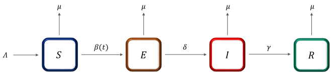
Figure 1: Compartmental diagram for the model.

Incorporating Seasonality in Disease Transmission

In Bangladesh, dengue transmission is heavily influenced by seasonal variations, particularly during the rainy season, when increased rainfall creates ideal conditions for Aedes aegypti mosquito breeding [23, 22]. To account for this seasonality in our model, we introduce a time-dependent transmission rate, $\beta(t)$, which captures the fluctuations in transmission driven by seasonal factors. $\beta(t)$ is modeled as a combination of a baseline transmission rate, $\beta_{np}$ (during non-rainy seasons), and a Gaussian peak transmission rate, $\beta_{p}$ (during rainy seasons), which then decays logistically back to baseline. Additionally, we include $A_{\beta}$ to denote the amplitude of the seasonal variation, $t_{p}$ to represent the peak time at the midpoint of the rainy season, and $\sigma$ to control the width of the seasonal peak. The functional form of $\beta(t)$ is given by:

$$\beta(t)=\beta_{np}+A_{\beta}\exp\left(-\frac{(t-t_{p})^{2}}{2\sigma^{2}}\right)+\frac{\beta_{p}}{1+\exp\left(\frac{t-t_{p}-\sigma}{\sigma}\right)}$$ (2)

The Gaussian component in (2) models the spike in cases, while the logistic decay accounts for the return to the endemic phase. Incorporating this seasonality allows the model to more accurately reflect the real-world dynamics of dengue transmission in Bangladesh (Fig. 2).

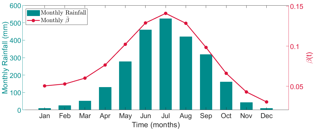
Figure 2: Time-varying transmission rate $\beta(t)$ and average monthly rainfall in Bangladesh over one year. $\beta(t)$ is evaluated using (2) with parameters $A_{\beta}=0.10$, $t_{p}=200$, $\sigma=60$, $\beta_{p}=0.03$, and $\beta_{np}=0.02$. Rainfall data for average monthly levels in Bangladesh in 2023 is collected from [24].

II-C Parameter Estimation through MCMC

To estimate the parameters of our model (1), we employ a Bayesian inference approach, utilizing the Metropolis-Hastings algorithm within the MCMC framework.

Priors and Likelihood

The prior distribution for each parameter $\theta$ is specified as follows:

$$\beta_{np}\sim U(0,1),\quad A_{\beta}\sim U(0,1),\quad\beta_{p}\sim U(0,1)$$

$$t_{p}\sim N(220,30),\quad\sigma\sim N(60,10),\quad\sigma_{obs}\sim\text{Exponential}(1)$$

The posterior distribution of the parameters, given the observed data $D$, is obtained using Bayes’ theorem:

$$P(\theta|D)=\frac{P(D|\theta)P(\theta)}{P(D)}$$

or alternatively:

$$P(\theta|D)\propto P(D|\theta)P(\theta)$$

where $P(D|\theta)$ is the likelihood function and $P(\theta)$ is the prior.

The likelihood function is constructed by comparing the observed daily dengue cases $D_{i}$ to the model-predicted cases $y(t_{i})$. Assuming Gaussian errors, the likelihood is given by:

$$L(\theta|D)=\prod_{i=1}^{T}\frac{1}{\sqrt{2\pi\sigma_{obs}^{2}}}\exp\left(-\frac{(D_{i}-y(t_{i}))^{2}}{2\sigma_{obs}^{2}}\right)$$

Model Predictions and Error Handling

The prediction error $E^{2}$ between the observed and predicted values is minimized during the MCMC sampling process,

$$E^{2}=\sum_{i=1}^{T}(D_{i}-y(t_{i}))^{2}$$

Assuming the errors are Gaussian, the likelihood function becomes $L(\theta|D)=\exp(-E^{2})$.

MCMC Sampling Details

We run four independent MCMC chains, each with 50,000 iterations and 5,000 warm-up iterations. Convergence is assessed using the Gelman-Rubin statistic $\hat{R}$, ensuring that the chains have mixed well and the variance between chains is similar to the variance within chains. The estimated parameters are presented in Table II, while the results of the posterior predictive check are illustrated in Figure 3.

II-D Time-Nonhomogeneous Stochastic Modeling

The CTMC-based SEIR model builds on the ODE-based model framework to formulate the infinitesimal transition probabilities for a time-nonhomogeneous stochastic process. For simplicity, the same notation that is used in the ODE model is applied to the CTMC model. The variables in the CTMC are discrete random variables where $E=0$ and $I=0$ are absorbing states: $S(t),E(t),I(t),R(t)\in{0,1,2,3,\dots,N},\quad t\in[0,\infty)$. Let $\Delta t\!>\!0$ be sufficiently small so that at most one event occurs during the interval $\Delta t$. Define $\mathbf{X}(t)=(S(t),E(t),I(t),R(t))$ and $\Delta\mathbf{X}(t)=(\Delta S(t),\Delta E(t),\Delta I(t),\Delta R(t))$, where, for example, $\Delta E(t)=E(t+\Delta t)-E(t)$, and similarly for the other states. The transition probabilities between states depend on both the current time $t$ and the elapsed time between events $\Delta t$, with transition rates summarized in Table I. For instance, the probability of a new infection occurring during event 4 in Table I within the time interval $\Delta t$ is given by: $\mathbb{P}\{\Delta\mathbf{X}(t)=(-1,1,0,0)\mid\mathbf{X}(t)\}=\beta(t)I\frac{S}{N}\Delta t+o(\Delta t)$

TABLE I: Transitions and rates in the CTMC-based model

Event	Description	State transition	Rate
1	Susceptible birth	$S\to S+1$	$\Lambda$
2	Susceptible death	$S\to S-1$	$\mu S$
3	Recovered death	$R\to R-1$	$\mu R$
4	Infection	$(S,E)\to(S-1,E+1)$	$\beta(t)I\frac{S}{N}$
5	Exposed death	$E\to E-1$	$\mu E$
6	Latent to infectious	$(E,I)\to(E-1,I+1)$	$\delta E$
7	Infected death	$I\to I-1$	$\mu I$
8	Infected recovery	$(I,R)\to(I-1,R+1)$	$\gamma I$

II-E Model Analysis

Basic and Seasonal Reproduction Numbers

When model parameters are constant, the basic reproduction number, $\mathcal{R}_{0}$, can be directly computed from the next generation matrix (NGM). This is done by analyzing the exposed and infectious stages of the system (1) through linearization around the Disease-Free Equilibrium (DFE), where $S=\Lambda/\mu=N$. The DFE remains stable in the absence of infection. In the NGM approach, the Jacobian matrix is decomposed into new infections, $F(t)$, and other transitions, $V(t)$, such that $J(t)=F(t)-V(t)$ [11, 12]:

$$F(t)=\begin{bmatrix}0&\beta(t)\\ 0&0\end{bmatrix},\quad V(t)=\begin{bmatrix}\delta+\mu&0\\ -\delta&\gamma+\mu\end{bmatrix}.$$

With a constant transmission rate, $\beta(t)\equiv\bar{\beta}$, the basic reproduction number, $\mathcal{R}_{0}$, is given by

$$\mathcal{R}_{0}=\rho(FV^{-1})=\frac{\bar{\beta}\delta}{(\delta+\mu)(\gamma+\mu)}.$$ (3)

When $\mathcal{R}_{0}>1$, the DFE is unstable, leading to an outbreak. If $\mathcal{R}_{0}<1$, the DFE is stable, and the disease dies out.

For systems with time-periodic transmission rates, Wang and Zhao’s approach using Floquet theory [13, 12] provides a more accurate representation of the seasonal reproduction number ($\mathcal{R}_{0}^{\text{seasonal}}$). For $X=(E,I)^{T}$, the linear system can be expressed as

$$\dot{X}=\left[F(t)-V(t)\right]X,\quad X(0)=I_{d}.$$

The maximum Floquet multiplier of the monodromy matrix, $\rho(X(\omega))$, corresponds to the basic reproduction number, $\mathcal{R}_{0}$. Since an explicit solution for $\mathcal{R}_{0}$ is generally unavailable, it is computed numerically by introducing a parameter $\lambda$ into the system:

$$\dot{X}=\left[\dfrac{F(t)}{\lambda}-V(t)\right]X,\quad X(0)=I_{d}.$$ (4)

An iterative sequence $\{\lambda_{i}\}$ is generated until it converges to a value $\lambda_{k}$ such that the spectral radius of the maximum Floquet multiplier is close to one, i.e., $|\rho(X(\omega,\lambda_{k}))-1|<10^{-6}$. The final value $\lambda_{k}$ approximates $\mathcal{R}_{0}^{\text{seasonal}}$. The stability of the DFE and the role of the constant and seasonal basic reproduction numbers as thresholds for disease outbreak are validated by verifying specific conditions [11, 12].

Probability of Disease Outbreak

To estimate the probability of a disease outbreak from the CTMC model, $n$ sample paths are simulated using a Monte Carlo approach to account for the stochastic nature of disease transmission and progression. Each path begins with 1 initial infected individual, and the simulation runs until one of two conditions is met: either the combined number of exposed and infected individuals ($E+I$) drops to 0, indicating disease extinction, or it reaches a predefined outbreak level (OL). The outbreak probability is calculated as the proportion of sample paths that lead to an outbreak, while the extinction probability is the proportion of paths that lead to extinction. If $n_{\text{ext}}$ represents the number of sample paths where extinction occurs, the extinction probability is given by $\mathbb{P}_{\text{ext}}={n_{\text{ext}}}/{n}$, and the outbreak probability is defined as $\mathbb{P}_{\text{outbreak}}=1-\mathbb{P}_{\text{ext}}$.

III Numerical Results

To ensure the reliability of our MCMC sampling, we assess convergence using the Gelman-Rubin diagnostic, also known as the $\hat{R}$ statistic, and calculated the Effective Sample Size (ESS) for each parameter.

The $\hat{R}$ values for all parameters are consistently close to 1.0, indicating proper convergence. In terms of the Effective Sample Size (ESS), all parameters has sufficiently large values, confirming that the number of independent samples is adequate for precise estimation of the posterior distributions. The ESS values are as follows: $A_{\beta}$ (47,560), $\beta_{np}$ (39,800), $\sigma$ (40,670), $\beta_{p}$ (40630), and $t_{p}$ (77,290).

Fig. 3 shows that the predicted values closely follow the observed data, especially around the peak of the dengue outbreak, indicating a good fit of the model. The 95% credible interval effectively captures the variability in the observed data, providing a measure of uncertainty around the predictions.

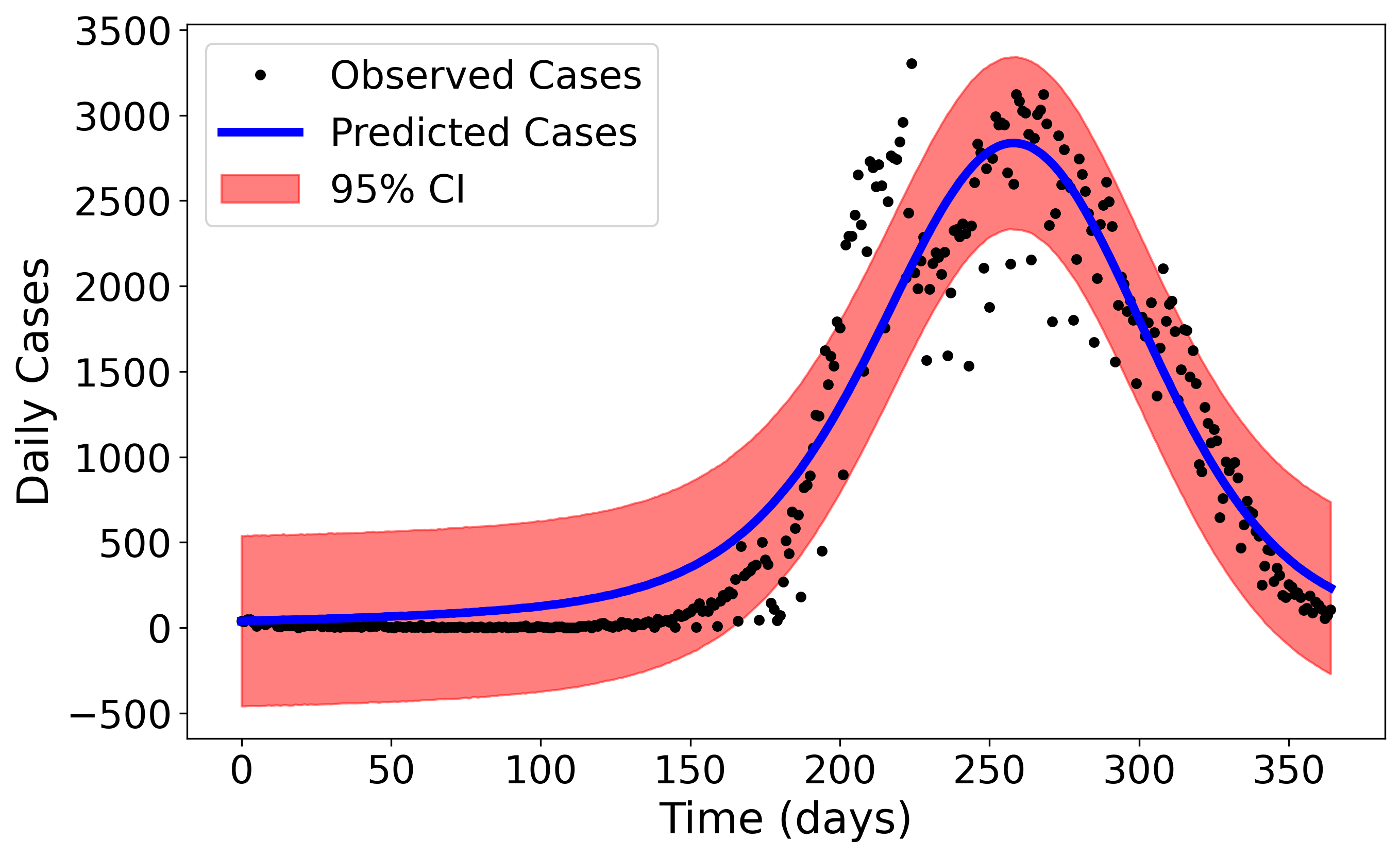
Figure 3: Posterior predictive check compares the observed daily dengue cases (black points) with the model’s predicted cases (blue line) along with the 95% credible interval (red shaded region).

The results presented in Table II summarize the posterior estimates of key parameters in the model. The non-peak transmission rate ($\beta_{np}$) is estimated with a mean value of 0.0566 and a 95% credible interval (CI) ranging from 0.0333 to 0.0741, which is consistent with literature [10] . The amplitude of seasonal variation ($A_{\beta}$) has a mean of 0.0470 and a 95% CI between 0.0415 and 0.0545, indicating moderate seasonal effects. The peak time ($t_{p}$) for dengue transmission is centered around 190.72 days, which corresponds to early July, aligning with the onset of the rainy season in Bangladesh, a critical period for increased mosquito breeding and dengue transmission.

TABLE II: Posterior Parameter Estimates for the SEIR Model

	Prior	Mean	95% CI
$\beta_{np}$	$U(0,1)$	0.0567	[0.033, 0.074]
$A_{\beta}$	$U(0,1)$	0.047	[0.042, 0.055]
$t_{p}$	$N(220,30)$	190.72	[190.02, 192.64]
$\sigma$	$N(60,10)$	61.817	[50.896, 75.117]
$\beta_{p}$	$U(0,1)$	0.085	[0.069, 0.105]
$\delta$	–	$0.25$ [10]	–
$\gamma$	–	$0.125$ [10]	–
$\mu$	–	$0.0000380$ [39]	–

In Fig. 4, the heatmaps illustrate how changes in model parameters affect the $\mathcal{R}_{0}^{\text{seasonal}}$. For a comprehensive analysis, we extend the model parameter values beyond the 95% confidence interval, but remain well within the range found in existing literature [10]. Furthermore, Fig. 5 demonstrates that varying the same parameters as in Fig. 4 (a) produces a similar pattern in the probability of outbreak heatmap, highlighting how our framework can generate consistent and comparable results from both deterministic and stochastic models.

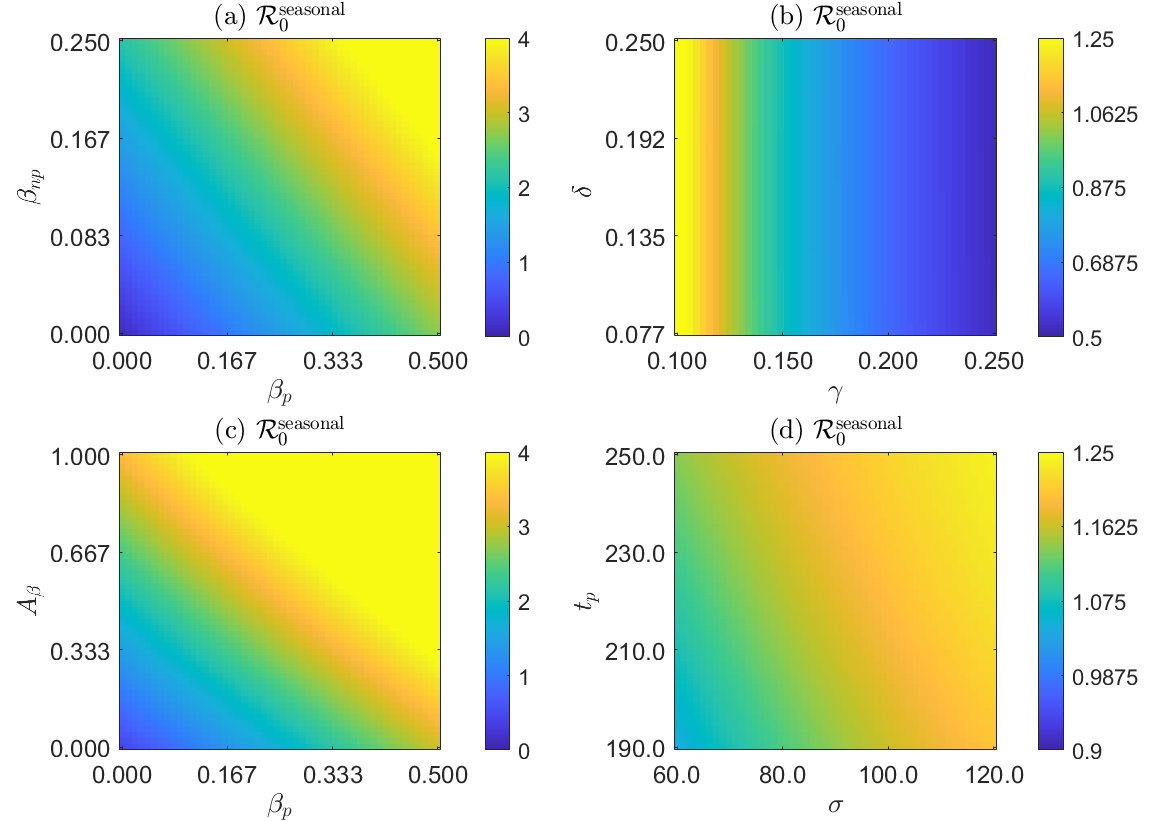
Figure 4: Impact of parameter variations on $\mathcal{R}_{0}^{\text{seasonal}}$ across four cases, with all other parameters held at their respective mean values from Table II.

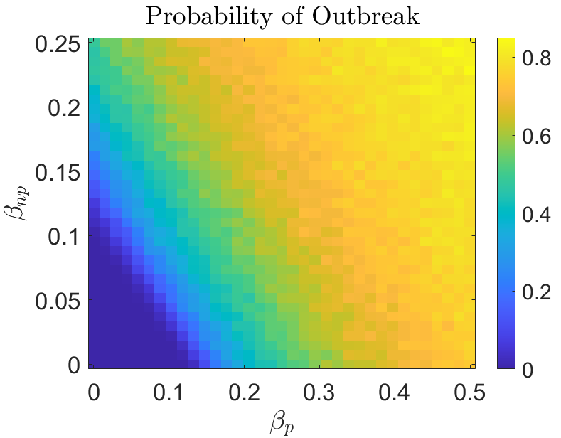
Figure 5: Impact of varying $\beta_{np}$ and $\beta_{p}$ on the probability of outbreak ($\mathbb{P}_{\text{outbreak}}$), with all other parameters held at their respective mean values from Table II, $n=1000$, and $OL=100$.

TABLE III: Comparison between basic $\mathcal{R}_{0}$, $\mathcal{R}_{0}^{\text{seasonal}}$, and $\mathbb{P}_{\text{outbreak}}$ as $\sigma$,$\beta_{np}$, and $\beta_{p}$ are varied, with $n=10000$, and $OL=100$

$\sigma$	$\beta_{np}$	$\beta_{p}$	$\bar{\beta}$	$\mathcal{R}_{0}$	$\mathcal{R}_{0}^{\text{seasonal}}$	$\mathbb{P}_{\text{outbreak}}$
60 days	0.057	0.085	0.132	1.059	1.045	0.113
75 days	0.057	0.085	0.139	1.108	1.097	0.137
120 days	0.057	0.085	0.151	1.205	1.202	0.185
60 days	0.074	0.105	0.163	1.306	1.290	0.300
75 days	0.074	0.105	0.170	1.358	1.347	0.309
120 days	0.074	0.105	0.183	1.460	1.456	0.330
60 days	0.057	0.581	0.463	3.704	3.578	0.765
75 days	0.057	0.581	0.479	3.827	3.743	0.784
120 days	0.057	0.581	0.505	4.036	4.003	0.809

IV Conclusion

This research aims to equip policymakers with a comprehensive mathematical framework to better understand disease dynamics and address the growing dengue crisis in Bangladesh. We incorporate the evident seasonality of dengue outbreak patterns into our model and propose an innovative transmission rate that reflects these seasonal variations. Our study demonstrates how Bayesian parameter estimation can guide both deterministic and stochastic SEIR frameworks, allowing for the comparison of key outbreak measures like basic and seasonal $\mathcal{R}_{0}$ and probability of outbreak, as shown in Table III, ultimately aiding in the mitigation of dengue infections.

References

- [1] Centers for Disease Control and Prevention, “About Dengue: What it is,” n.d. [Online]. Available: https://www.cdc.gov/dengue/about/index.html. [Accessed: July 31, 2024].
- [2] M. E. H. Kayesh, I. Khalil, M. Kohara, and K. Tsukiyama-Kohara, “Increasing dengue burden and severe dengue risk in Bangladesh: an overview,” Tropical Medicine and Infectious Disease, vol. 8, no. 1, p. 32, 2023.
- [3] C. J. Struchiner, J. Rocklöv, A. Wilder-Smith, and E. Massad, “Increasing dengue incidence in Singapore over the past 40 years: population growth, climate and mobility,” PloS one, vol. 10, no. 8, p. e0136286, 2015.
- [4] A. Wilder-Smith, E.-E. Ooi, S. G. Vasudevan, and D. J. Gubler, “Update on dengue: epidemiology, virus evolution, antiviral drugs, and vaccine development,” Current infectious disease reports, vol. 12, pp. 157–164, 2010.
- [5] C. P. Simmons, J. J. Farrar, N. van Vinh Chau, and B. Wills, “Dengue,” New England Journal of Medicine, vol. 366, no. 15, pp. 1423–1432, 2012.
- [6] World Health Organization, “Dengue and Severe Dengue,” 2023. [Online]. Available: https://www.who.int/news-room/fact-sheets/detail/dengue-and-severe-dengue. [Accessed: July 31, 2024].
- [7] E. B. Yunus, A. M. Bangali, M. Mahmood, M. M. Rahman, A. R. Chowdhury, and K. R. Talukder, “Dengue Outbreak 2000 in Bangladesh: From Speculation to Reality and Exercises,” World Health Organization, Regional Office for South-East Asia, 2001.
- [8] Directorate General of Health Services, Bangladesh, “Dengue Situation Report, 2019,” 2019. [Online]. Available: https://old.DGHS2023.gov.bd/images/docs/Notice/2019/dengue/Dengue20191231.pdf. [Accessed: July 31, 2024].
- [9] M. Chan and M. A. Johansson, “The incubation periods of dengue viruses,” PloS one, vol. 7, no. 11, p. e50972, 2012.
- [10] A. Pandey, A. Mubayi, and J. Medlock, “Comparing vector–host and SIR models for dengue transmission,” Mathematical biosciences, vol. 246, no. 2, pp. 252–259, 2013.
- [11] P. van den Driessche and J. Watmough, “Reproduction numbers and sub-threshold endemic equilibria for compartmental models of disease transmission,” Mathematical Biosciences, vol. 180, no. 1-2, pp. 29–48, 2002.
- [12] W. Wang and X.-Q. Zhao, “Threshold dynamics for compartmental epidemic models in periodic environments,” Journal of Dynamics and Differential Equations, vol. 20, pp. 699–717, 2008.
- [13] C. A. Klausmeier, “Floquet Theory: a Useful Tool for Understanding Nonequilibrium Dynamics,” Theoretical Ecology, vol. 1, pp. 152-161, 2008.
- [14] Directorate General of Health Services, Bangladesh, “Dengue Situation Report, 2019,” 2019. [Online]. Available: https://old.DGHS2023.gov.bd/images/docs/Notice/2019/dengue/Dengue20191231.pdf. [Accessed: July 31, 2024].
- [15] World Health Organization, “Ten threats to global health in 2019,” 2019. [Online]. Available: https://www.who.int/news-room/spotlight/ten-threats-to-global-health-in-2019. [Accessed: August 27, 2024].
- [16] World Health Organization, “Dengue - Global Situation Update,” 2024. [Online]. Available: https://www.who.int/emergencies/disease-outbreak-news/item/2024-DON518. [Accessed: August 27, 2024].
- [17] World Health Organization, “Dengue and Severe Dengue,” 2023. [Online]. Available: https://www.who.int/news-room/fact-sheets/detail/dengue-and-severe-dengue. [Accessed: August 27, 2024].
- [18] M. S. Hossain, A. A. Noman, S. M. Mamun, and A. A. Mosabbir, “Twenty-two years of dengue outbreaks in Bangladesh: epidemiology, clinical spectrum, serotypes, and future disease risks,” Tropical Medicine and Health, vol. 51, no. 1, pp. 1–14, 2023.
- [19] M. A. Aziz, J. R. Gorham, and M. B. Gregg, “Dacca fever”-an outbreak of dengue,” 1967.
- [20] A. S. Mahmud, J. Bhattacharjee, R. E. Baker, and P. P. Martinez, “Alarming trends in dengue incidence and mortality in Bangladesh,” The Journal of infectious diseases, vol. 229, no. 1, pp. 4–6, 2024.
- [21] M. A. Rob, M. Hossain, M. A. Sattar, I. U. Ahmed, A. F. M. N. Chowdhury, H. M. H. Mehedi, N. Mohammed, M. M. Quader, M. Z. Hossain, M. Rahman, et al., “Circulating dengue virus serotypes, demographics, and epidemiology in the 2023 dengue outbreak in Chittagong, Bangladesh,” European Journal of Microbiology and Immunology, 2024.
- [22] E. P. Pliego, J. Velázquez-Castro, and A. F. Collar, “Seasonality on the life cycle of Aedes aegypti mosquito and its statistical relation with dengue outbreaks,” Applied Mathematical Modelling, vol. 50, pp. 484–496, 2017.
- [23] I. Morales, H. Salje, S. Saha, and E. S. Gurley, “Seasonal distribution and climatic correlates of dengue disease in Dhaka, Bangladesh,” The American journal of tropical medicine and hygiene, vol. 94, no. 6, p. 1359, 2016.
- [24] Bangladesh Meteorological Department, “Normal Monthly Rainfall,” 2023. [Online]. Available: https://live6.bmd.gov.bd//p/Normal-Monthly-Rainfall. [Accessed: August 28, 2024].
- [25] Z. Feng and J. X. Velasco-Hernández, “Competitive exclusion in a vector-host model for the dengue fever,” Journal of mathematical biology, vol. 35, pp. 523–544, 1997.
- [26] M. Aguiar, V. Anam, K. B. Blyuss, C. D. S. Estadilla, B. V. Guerrero, D. Knopoff, B. W. Kooi, A. K. Srivastav, V. Steindorf, and N. Stollenwerk, “Mathematical models for dengue fever epidemiology: A 10-year systematic review,” Physics of Life Reviews, vol. 40, pp. 65–92, 2022.
- [27] L. Esteva and C. Vargas, “Analysis of a dengue disease transmission model,” Mathematical Biosciences, vol. 150, no. 2, pp. 131–151, 1998.
- [28] R. M. Anderson and R. M. May, “Infectious diseases of humans: dynamics and control,” Philosophical Transactions of the Royal Society of London. Series B: Biological Sciences, vol. 336, no. 1277, pp. 159–164, 1992.
- [29] M. Aguiar, V. Anam, K. B. Blyuss, C. D. S. Estadilla, B. V. Guerrero, D. Knopoff, B. W. Kooi, A. K. Srivastav, V. Steindorf, and N. Stollenwerk, “Mathematical models for dengue fever epidemiology: A 10-year systematic review,” Physics of Life Reviews, vol. 40, pp. 65–92, 2022.
- [30] T.-T. Zheng and L.-F. Nie, “Modelling the transmission dynamics of two-strain Dengue in the presence awareness and vector control,” Journal of theoretical biology, vol. 443, pp. 82–91, 2018.
- [31] M. Aguiar, N. Stollenwerk, and B. W. Kooi, “Epidemiology of dengue fever: a model with temporary cross-immunity and possible secondary infection shows bifurcations and chaotic behaviour in wide parameter regions,” Mathematical Modelling of Natural Phenomena, vol. 3, no. 7, pp. 48–70, 2008.
- [32] Centers for Disease Control and Prevention, “Dengue: About Dengue,” 2024. [Online]. Available: https://www.cdc.gov/dengue/about/index.html. [Accessed: August 28, 2024].
- [33] T. A. Perkins, T. W. Scott, A. Le Menach, and D. L. Smith, “Heterogeneity, Mixing, and the Spatial Scales of Mosquito-Borne Pathogen Transmission,” Proceedings of the National Academy of Sciences, vol. 103, no. 42, pp. 15824–15829, 2006.
- [34] K. F. Nipa, S. R.-J. Jang, and L. J. S. Allen, “The effect of demographic and environmental variability on disease outbreak for a dengue model with a seasonally varying vector population,” Mathematical Biosciences, vol. 331, p. 108516, 2021.
- [35] M. H. Riad, L. W. Cohnstaedt, and C. M. Scoglio, “Risk assessment of dengue transmission in Bangladesh using a spatiotemporal network model and climate data,” The American journal of tropical medicine and hygiene, vol. 104, no. 4, p. 1444, 2021.
- [36] M. Asaduzzaman, A. Kilicman, A. -A. Mamun, and M. D. Hossain, “Analysis of a Novel Conformable Fractional Order ASIR Dengue Transmission Model in the Perspective of Bangladesh,” Mathematical Models and Computer Simulations, vol. 16, no. 3, pp. 431–456, 2024.
- [37] M. N. Hasan, I. Khalil, M. A. B. Chowdhury, M. Rahman, M. Asaduzzaman, M. Billah, L. A. Banu, M.-U. Alam, A. Ahsan, T. Traore, et al., “Two decades of endemic dengue in Bangladesh (2000–2022): trends, seasonality, and impact of temperature and rainfall patterns on transmission dynamics,” Journal of Medical Entomology, vol. 61, no. 2, pp. 345–353, 2024.
- [38] K. M. Rahman, Y. Sharker, R. A. Rumi, M.-U. I. Khan, M. S. Shomik, M. W. Rahman, S. M. Billah, M. Rahman, P. K. Streatfield, D. Harley, et al., “An association between rainy days with clinical dengue fever in Dhaka, Bangladesh: findings from a hospital based study,” International Journal of Environmental Research and Public Health, vol. 17, no. 24, p. 9506, 2020.
- [39] World Health Organization, “Bangladesh: WHO Data,” 2024. [Online]. Available: https://data.who.int/countries/050. [Accessed: August 31, 2024].
- [40] Directorate General of Health Services, Bangladesh, “Dengue Dashboard,” 2023. [Online]. Available: https://dashboard.DGHS2023.gov.bd/pages/heoc_dengue_v1.php. [Accessed: Aug. 28, 2024].