Evaluating Deep Regression Models for WSI-Based Gene-Expression Prediction

Abstract

Prediction of mRNA gene-expression profiles directly from routine whole-slide images (WSIs) using deep learning models could potentially offer cost-effective and widely accessible molecular phenotyping. While such WSI-based gene-expression prediction models have recently emerged within computational pathology, the high-dimensional nature of the corresponding regression problem offers numerous design choices which remain to be analyzed in detail. This study provides recommendations on how deep regression models should be trained for WSI-based gene-expression prediction. For example, we conclude that training a single model to simultaneously regress all $20\thinspace 530$ genes is a computationally efficient yet very strong baseline.

Molecular phenotyping via mRNA gene-expression profiling is an important tool for providing prognostic information in cancer precision medicine [28, 27, 17, 24]. While molecular phenotyping remains relatively expensive and time-consuming, techniques for predicting gene-expression profiles from routinely available hematoxylin and eosin (H&E)-stained whole-slide images (WSIs) have recently emerged within the computational pathology domain [26, 31, 32, 19, 33]. Such deep learning models for WSI-based gene-expression prediction could potentially be used to, for example, pre-screen large cohorts of patients to identify those most likely to benefit from detailed molecular phenotyping. However, there are various different ways in which WSI-based gene-expression prediction models could be designed and trained. In particular, gene-expression profiles consists of continuous measurements of a large number of genes, making gene-expression prediction an extremely high-dimensional regression problem. Various different deep regression approaches have been explored in the general machine learning literature [13, 6], and contrastive learning-based approaches designed specifically for spatial gene-expression prediction have also emerged [18, 8]. Currently, it is unclear which of these numerous different regression approaches are most well-suited for gene-expression prediction. The high-dimensional nature of the gene-expression regression problem also offers further design choices which remain to be studied in detail. For example, it is unclear whether separate regression models should be trained for each individual gene [31], or if a single model regressing all genes can provide comparable prediction accuracy. In this work we therefore study some of these open questions, providing recommendations on how deep regression models should be trained for WSI-based gene-expression prediction.

[width=0.9225]figures/main_results4_std_pearson [width=0.9225]figures/main_results4_std_pearson_top1k [width=0.9225]figures/main_results4_std_num_geq_04

Figure 1: Model performance comparison of the four regression models across the four TCGA datasets, when utilizing both UNI and Resnet-IN as patch-level feature extractors. Top: mean Pearson correlation of all $N=20\thinspace 530$ genes. Middle: mean Pearson correlation of the top $1\thinspace 000$ genes with the highest regression accuracy. Bottom: The number of genes (out of the $N=20\thinspace 530$ total number of genes) regressed with a Pearson correlation of at least $0.4$. Higher is better for all three metrics. All results are mean$\pm$std (standard deviation) over the 5 cross-validation folds. Raw numerical results for this figure are provided in Table S1 - S4 in the supplementary material. The same model performance comparison but using Spearman correlation metrics instead of Pearson is also found in Figure S1.

Figure 2: Performance comparison across the four TCGA datasets when multiple UNI - Direct - ABMIL models are used to output a full predicted gene-expression profile $\hat{y}(x)\in\mathbb{R}^{N}$ for each WSI $x$, using either sequential chunking or clustering to group the $N\!=\!20\thinspace 530$ genes into subsets. Same metrics as in Figure 1. All results are the mean over the 5 cross-validation folds.

Figure 3: Performance comparison across the four TCGA datasets when progressively increasing the number of genes regressed per UNI - Direct - ABMIL model, using sequential chunking to group genes into subsets. All models are evaluated only on the subset of the first $800$ genes (to make this evaluation computationally manageable). Same metrics as in Figure 1, except the middle row shows the mean Pearson correlation of the top $50$ genes with the highest regression accuracy. All results are the mean over the 5 cross-validation folds.

We conduct experiments on datasets from the Cancer Genome Atlas (TCGA), for four different cancer types: breast (TCGA-BRCA, $n\!=\!1\thinspace 062$ patients), head-neck (TCGA-HNSC, $n\!=\!450$), stomach (TCGA-STAD, $n\!=\!416$) and bladder (TCGA-BLCA, $n\!=\!386$). For each dataset, we train deep regression models to output gene-level transcription estimates of $N\!=\!20\thinspace 530$ genes (utilizing gene-expression data from UCSC Xena [5]) from the corresponding diagnostic H&E WSI. Models are trained and evaluated using 5-fold site-aware cross-validation [9]. We compare four different types of regression models, all based on patch-level feature vectors extracted from the WSI using frozen UNI [1] or Resnet-IN models (see the Methods section for details). 1. Direct - ABMIL uses attention-based multiple instance learning (ABMIL) [10, 12] to directly output a predicted gene-expression profile $\hat{y}(x)\in\mathbb{R}^{N}$ for the WSI $x$. 2. Direct - Patch-Level removes the trainable ABMIL aggregator and computes $\hat{y}(x)\in\mathbb{R}^{N}$ as the mean over patch-level predictions. 3. Contrastive instead utilizes contrastive learning [2, 23] to align WSI and gene-expression representations, and computes $\hat{y}(x)\in\mathbb{R}^{N}$ as a linear combination of the most similar gene-expression profiles from the train set. 4. kNN is a simple baseline model (with no trainable parameters) utilizing the k-nearest neighbors algorithm. We also evaluate how the accuracy is affected if, instead of training a single model to regress all $N\!=\!20\thinspace 530$ genes, multiple models are separately trained to regress subsets of genes and then combined at test-time to output a full predicted gene-expression profile $\hat{y}(x)\in\mathbb{R}^{N}$. The $N\!=\!20\thinspace 530$ genes are grouped into subsets either via sequential chunking, or clustering of correlated genes.

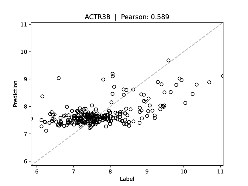
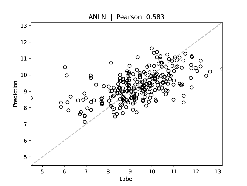
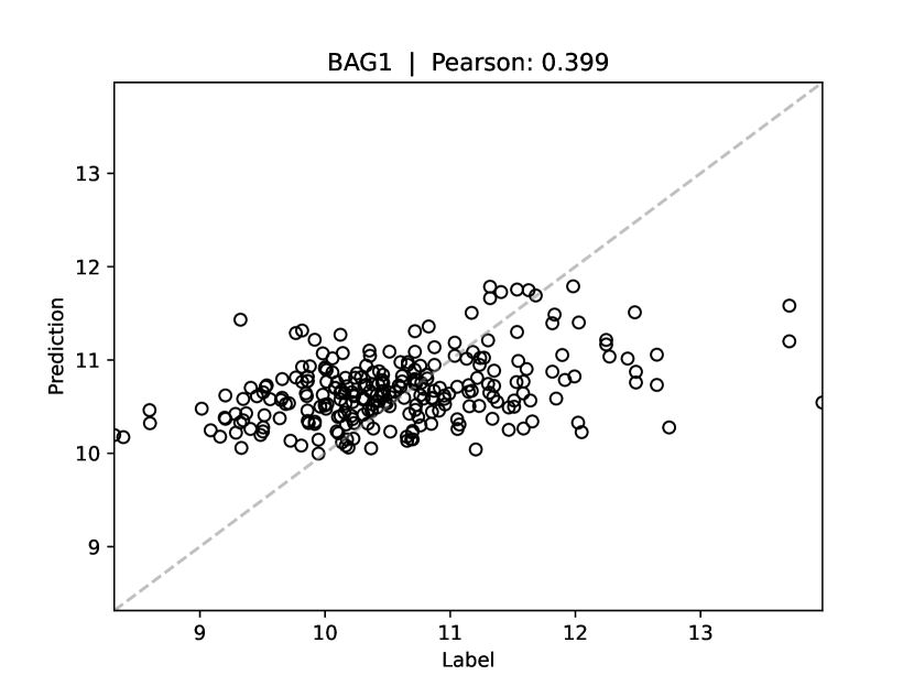
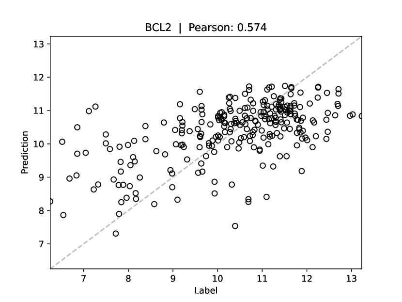
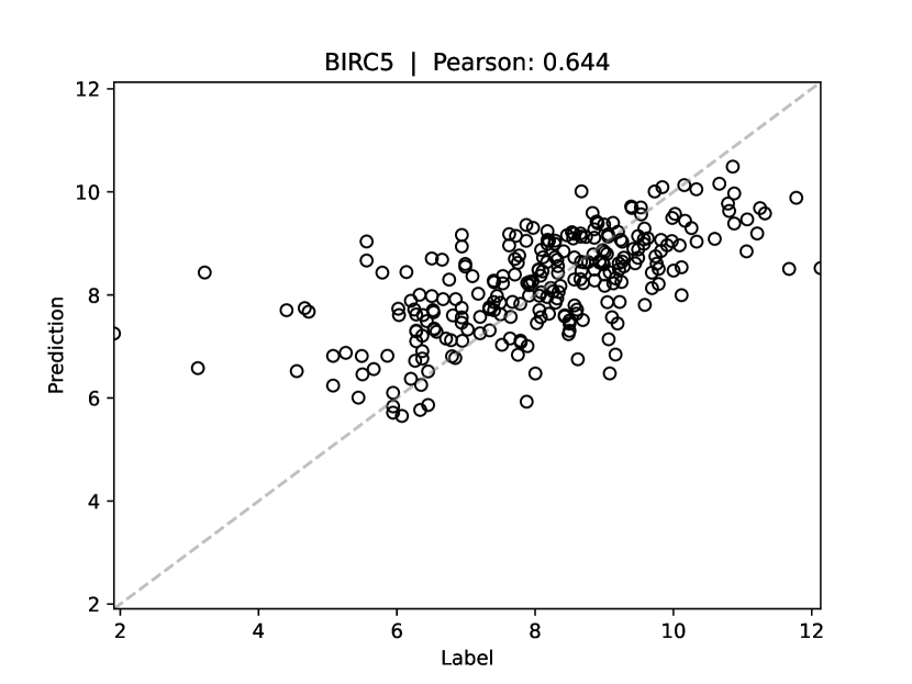
Figure S4: Correlation plots showing predicted vs ground-truth gene-expression values for PAM50 gene 1 - 5, for the UNI - Direct - ABMIL model on the TCGA-BRCA dataset, for the test split of the first cross-validation fold.

The performance of the four regression models, when utilizing both UNI and Resnet-IN as patch-level feature extractors, is compared in Figure 1. First, we observe that UNI consistently outperforms Resnet-IN across all models and datasets. Among the four models, kNN clearly achieves the worst performance. Moreover, Direct - Patch-Level is slightly outperformed by both Direct - ABMIL and Contrastive. With UNI, Direct - ABMIL and Contrastive are difficult to separate. With Resnet-IN, Contrastive consistently outperforms all other models. We also note that UNI - Direct - ABMIL regresses $4\thinspace 927\pm 357$ out of the $N=20\thinspace 530$ genes with a Pearson correlation of at least $0.4$ on TCGA-BRCA, $3\thinspace 987\pm 765$ genes on TCGA-HNSC, $3\thinspace 240\pm 1342$ genes on TCGA-STAD, and $4\thinspace 364\pm 1188$ genes on TCGA-BLCA. Figure S2 in the supplementary material shows the same model comparison, but when evaluated only on a subset of 50 genes (PAM50) with demonstrated prognostic value for breast cancer [20, 30]. We observe a virtually identical ranking of the four regression models, and note that UNI - Direct - ABMIL regresses the PAM50 genes with a mean Pearson correlation of $0.562\pm 0.020$ on TCGA-BRCA. The accuracy of UNI - Direct - ABMIL for each of the individual PAM50 genes on TCGA-BRCA is further listed in Table S8 ($13$ genes with a Pearson correlation of at least $0.65$), and Figure S4 - S7 show corresponding correlation plots. Lastly, Table S6 & S7 list the top $20$ genes (out of all $N=20\thinspace 530$) with the highest regression accuracy for UNI - Direct - ABMIL and UNI - Contrastive, across the four datasets. Here, we note that $5$ of the PAM50 genes (FOXA1, MLPH, ESR1, CCNE1 and ORC6L) are among the top $20$ on TCGA-BCRA for both models.

Figure 2 shows how the performance is affected (across the four datasets) when multiple UNI - Direct - ABMIL models are used to output a full predicted gene-expression profile $\hat{y}(x)\in\mathbb{R}^{N}$ for each WSI $x$. When increasing the number of models from a single one to more than $500$, we observe slight improvements on TCGA-STAD and TCGA-BLCA, and effectively no difference on TCGA-BRCA or TCGA-HNSC. On TCGA-BRCA, the mean Pearson correlation is even slightly decreased with more models. Also, we observe no clear difference in performance between the sequential chunking or clustering of genes. The performance of multiple UNI - Direct - ABMIL models is further studied in Figure 3. There, we start with the extreme case of training one model for each individual gene, and then progressively increase the number of genes per model, ending with the standard case of a single model regressing all $N=20\thinspace 530$ genes. In order to make this evaluation computationally manageable, we evaluate all models only on the subset of the first $800$ genes (for the extreme case of one gene per model, we thus have to train $800$ models instead of $20\thinspace 530$). We observe that, while the optimal number of genes per model varies slightly across different datasets and metrics, it is never optimal to train one model for each individual gene. Instead, the performance always improves when increasing the number of genes per model from $1$ to $10$, and from $10$ to $20$. The performance then eventually either peaks or levels off. Similar results are also obtained when training UNI - Direct - ABMIL models only on the PAM50 subset of genes on TCGA-BRCA, as shown in Table S5. When progressively increasing the number of genes per model from one ($50$ models, each regressing one gene) to $50$ (a single model regressing all PAM50 genes), the performance is consistently improved from a mean Pearson correlation of $0.560\pm 0.020$ to $0.576\pm 0.020$. Training separate models for each individual PAM50 gene is not even outperforming the standard UNI - Direct - ABMIL model trained to regress all $N=20\thinspace 530$ genes (mean Pearson correlation of $0.562\pm 0.020$ on PAM50).

The strong performance of UNI compared to Resnet-IN is expected but still encouraging, as it further demonstrates the value of pathology-specific feature extractors. In Figure 1 it can even be observed that UNI - kNN (the simplest possible baseline with no trainable components) outperforms Resnet-IN - Direct - ABMIL on most datasets. For the PAM50 genes on TCGA-BRCA, the performance of Direct - ABMIL is also significantly improved (from $0.373\pm 0.070$ to $0.562\pm 0.020$ in mean Pearson correlation, Table S5) by simply using UNI instead of Resnet-IN. When comparing the overall performance of the four regression models, the simple kNN baseline unsurprisingly ranks last by a significant margin. Comparing Direct - ABMIL and Direct - Patch-Level demonstrates a slight yet consistent added benefit of the trainable ABMIL aggregator. Direct - ABMIL and Contrastive achieve very similar performance with UNI, whereas the strong performance of Contrastive with Resnet-IN suggests that it might be more robust to the quality of the underlying patch-level feature extractor. In conclusion, it is difficult to declare a single clear winner or go-to model. Instead, our recommendation is that both Direct - ABMIL and Contrastive should be considered. From the experiments on using multiple UNI - Direct - ABMIL models (Figure 2 & 3, Table S5), the low performance of single-gene models is quite surprising. As this approach of training one model for each individual gene also corresponds to an extremely high computational cost, our study thus provides no reason for why it should be utilized in any practical application. Overall, using more than just a single model to predict $\hat{y}(x)\in\mathbb{R}^{N}$ gives modest performance gains at best. While the added computational cost of using multiple models might be worth the improved performance on TCGA-BLCA or TCGA-HNSC, this is likely not the case on TCGA-BRCA or TCGA-HNSC. Our experiments thus suggest that training a single model to regress all $N=20\thinspace 530$ genes is a very strong baseline. Therefore, given a particular dataset, our recommendation is to always start by training a single model (either Direct - ABMIL or Contrastive) and e.g. $10$ models with sequential chunking, and then explore multiple models further only if clear performance gains are observed in this initial experiment.

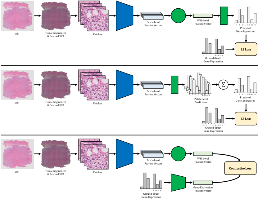
Figure 4: Overview of the three main evaluated models: Top: Direct - ABMIL. Middle: Direct - Patch-level. Bottom: Contrastive. All three models utilize the same initial WSI processing steps. First, the input WSI $x$ is tissue-segmented and divided into non-overlapping patches $\tilde{x}_{i}$ of size $256\times 256$ using CLAM [15]. Next, a feature vector $p(\tilde{x}_{i})$ is extracted for each patch, using a pretrained and frozen feature extractor (either UNI [1] or Resnet-IN). The different models then process these patch-level feature vectors $p(\tilde{x}_{i})$ further (see the Methods section for details), finally outputting a predicted gene-expression profile $\hat{y}(x)\in\mathbb{R}^{N}$ for all $N=20\thinspace 530$ genes. In all three figures, blue marks the pretrained and frozen feature extractor, whereas green marks trainable model components.

The main actionable takeaways from our study can be summarized as follows: 1. Utilizing the pathology-specific UNI as patch-level feature extractor clearly outperforms Resnet-IN. 2. Training regression models on top of UNI features gives accurate WSI-based models for gene-expression prediction (TCGA-BRCA: $4\thinspace 927$ genes with Pearson $\geq 0.4$, mean Pearson of $0.562$ for PAM50 genes). 3. Despite conceptual differences, Direct - ABMIL and Contrastive achieve very similar performance and should both be considered go-to models. 4. Training a single model to regress all $N=20\thinspace 530$ genes is a computationally efficient and very strong baseline, this should be the starting point given any new dataset. 5. Training one model for each individual gene incurs an extremely high computational cost yet achieves comparatively low regression accuracy.

While our evaluation based on site-aware cross-validation should give a more accurate account of model performance than standard cross-validation, it would be valuable to validate our findings further on external data in future work. More pathology-specific foundation models [16, 34, 29] could also be utilized as the underlying patch-level feature extractor, to determine whether Contrastive actually is more robust to this choice compared to Direct - ABMIL. Lastly, the surprisingly low performance of single-gene models could be analyzed further, trying to understand the mechanisms for why it instead is beneficial to regress multiple genes with each model.

Methods

Experimental Setup

We conduct experiments on four TCGA datasets: breast invasive carcinoma (TCGA-BRCA), head-neck squamous cell carcinoma (TCGA-HNSC), stomach adenocarcinoma (TCGA-STAD) and urothelial bladder carcinoma (TCGA-BLCA). We match WSIs with gene-expression data from UCSC Xena [5]. Specifically, we use the gene expression RNAseq - IlluminaHiSeq data, containing gene-level transcription estimates of $N=20\thinspace 530$ genes. This results in $1\thinspace 129$ total WSIs with matched gene-expression data for TCGA-BRCA, $464$ WSIs for TGCA-HNSC, $391$ WSIs for TCGA-STAD and $452$ WSIs for TCGA-BLCA. All models are trained and evaluated using 5-fold site-aware cross-validation (models are never trained and evaluated on samples from the same TCGA data collection site), in order to give a more fair account of model performance [9].

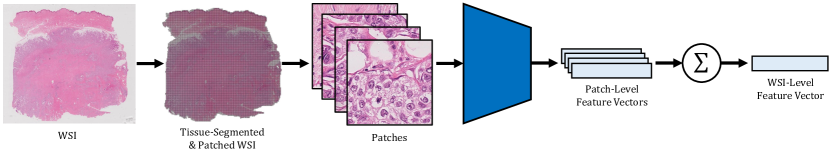
Figure 5: Overview of the simple kNN baseline, which contains no trainable model parameters. For the input WSI $x$, a WSI-level feature vector $w(x)$ is directly computed as the mean over the patch-level feature vectors $p(\tilde{x}_{i})$. kNN with $k=100$ is then utilized to output a predicted gene-expression profile $\hat{y}(x)\in\mathbb{R}^{N}$.

Model Overview

We evaluate three main different types of regression models (Figure 4), along with a simple kNN baseline (Figure 5). All four models take a WSI $x$ as input and output a predicted gene-expression profile $\hat{y}(x)\in\mathbb{R}^{N}$. Note that models thus output predicted values for all $N=20\thinspace 530$ genes, making this an extremely high-dimensional regression problem.

All four models also utilize the same initial WSI processing steps. First, the input WSI $x$ is tissue-segmented and divided into $P$ non-overlapping patches $\{\tilde{x}_{i}\}_{i=1}^{P}$ of size $256\times 256$ (at $20\times$ magnification) using CLAM [15]. The number of extracted tissue patches $P$ varies for different WSIs, with a typical range of $100-10\thinspace 000$ per WSI. Next, a feature vector $p(\tilde{x}_{i})$ (of dimension $1\thinspace 024$) is extracted for each patch $\tilde{x}_{i}$, using a pretrained and frozen feature extractor. The four models then process these patch-level feature vectors $\{p(\tilde{x}_{i})\}_{i=1}^{P}$ further, finally outputting a predicted gene-expression profile $\hat{y}(x)\in\mathbb{R}^{N}$.

Feature Extractors

We utilize two different patch-level feature extractors: UNI and Resnet-IN. UNI [1] is a ‘foundation model’, i.e. a deep learning model trained on large amounts of unlabeled data using self-supervised learning, developed specifially for the computational pathology domain. It is a vision transformer (ViT-Large) [3], pretrained using DINOv2 [21] on a pan-cancer dataset (20 major tissue types) collected from the Massachusetts General Hospital, Brigham & Women’s Hospital and the Genotype-Tissue Expression consortium. The dataset contains roughly $100$ million tissue patches from more than $100\thinspace 000$ WSIs.

Resnet-IN is a Resnet-50 model [7] pretrained on the ImageNet dataset [25] of natural images. Resnet-IN is included as a simple baseline, expected to be outperformed by the pathology-specific UNI. Both feature extractors are kept frozen in all our experiments, i.e. they are not updated during the training of any of the regression models.

Direct Regression Models

We evaluate two types of direct regression models, in which networks are trained to directly output a predicted gene-expression profile $\hat{y}(x)\in\mathbb{R}^{N}$ from the patch-level feature vectors. The networks are trained by minimizing the L2 loss between predicted and true gene-expression, $\|y-\hat{y}(x)\|^{2}$.

ABMIL

The first direct regression model, Direct - ABMIL in Figure 4 (top), utilizes an ABMIL model [10] to aggregate the set of patch-level feature vectors $\{p(\tilde{x}_{i})\}_{i=1}^{P}$ into a single WSI-level feature vector $w(x)$. This feature vector $w(x)$ is then fed as input to a small network head of two layers, finally outputting $\hat{y}(x)\in\mathbb{R}^{N}$. Both the ABMIL aggregator and the network head are trained using the L2 loss $\|y-\hat{y}(x)\|^{2}$.

Our ABMIL implementation is based on CLAM [15] (without the instance-level clustering), and we set the model and training hyperparameters according to UNI (see Methods - Weakly supervised slide classification in [1]). Specifically, models are trained using the AdamW optimizer [14] with a cosine learning rate schedule, for a maximum of 20 epochs. For each of the 5 folds, we split the training split further into train and val (random $90\%$ - $10\%$ split), and perform early stopping using the val loss.

Sequential Chunking  Since the regression problem is extremely high-dimensional ($N=20\thinspace 530$ genes), we also conduct experiments where multiple Direct - ABMIL models are used to output a full predicted gene-expression profile $\hat{y}(x)\in\mathbb{R}^{N}$ for any given WSI $x$. If using five models, for example, we separately train one Direct - ABMIL model that regresses the first $20530/5=4106$ genes, one model that regresses the next $4106$ genes, and similarly for the three other models. The only modification of the Direct - ABMIL model is to change the output dimension of the network head from $20\thinspace 530$ to $4\thinspace 106$. In the extreme case, $N=20\thinspace 530$ models could be trained (at a very high computational cost), each regressing a single gene.

Clustering  Instead of just sequentially dividing the $N=20\thinspace 530$ genes into chunks, and training models to regress all genes in each chunk, we also utilize k-means clustering (on the train split) to first group the genes into $k$ clusters. Then, we separately train one Direct - ABMIL model that regresses all genes in the first cluster, one model that regresses all genes in the second cluster, and similarly for all remaining clusters.

Patch-Level

The second direct regression model, Direct - Patch-Level in Figure 4 (middle), simplifies Direct - ABMIL by removing the trainable ABMIL WSI-level aggregator. Instead, each patch-level feature vector $p(\tilde{x}_{i})$ is directly fed as input to the small network head, outputting a predicted gene-expression profile $\hat{y}(\tilde{x}_{i})\in\mathbb{R}^{N}$ for each tissue patch $\tilde{x}_{i}$ in the WSI $x$. Then, the mean over these patch-level predictions $\{\hat{y}(\tilde{x}_{i})\}_{i=1}^{P}$ is computed, and output as the final WSI-level predicted gene-expression $\hat{y}(x)\in\mathbb{R}^{N}$. Compared to Direct - ABMIL, this model contains fewer trainable parameters. Moreover, it enables extraction of patch-level predictions, which potentially could be utilized for spatial analysis.

Contrastive Learning-Based Model

The third main evaluated regression model, Contrastive in Figure 4 (bottom), is conceptually quite different compared to the previous direct regression models. Instead of training networks to directly output a predicted gene-expression profile $\hat{y}(x)\in\mathbb{R}^{N}$ via the L2 loss, the contrastive learning-based model first trains networks to align WSI and gene-expression feature representations using a contrastive loss. Given a WSI $x$, a predicted gene-expression profile $\hat{y}(x)\in\mathbb{R}^{N}$ is then obtained by computing the similarity between the WSI representation and all gene-expression representations of the train set.

Our contrastive learning-based model is a relatively straightforward extension of the TANGLE method [11] proposed for WSI representation learning, applying it to the gene-expression prediction task. It can also be considered an extension of previous work [33, 18] utilizing contrastive learning for spatial gene-expression prediction based on spatial transcriptomics datasets.

Model Architecture & Training

We use the TANGLE model [11]. Just like the previous Direct - ABMIL, TANGLE utilizes an ABMIL model to aggregate patch-level feature vectors $\{p(\tilde{x}_{i})\}_{i=1}^{P}$ into a single WSI-level feature vector $w(x)$. It also consists of a gene-expression encoder model, which takes a gene-expression profile $y\in\mathbb{R}^{N}$ as input and compresses it into a feature vector $g(y)$, matching the dimension of the WSI-level feature vector $w(x)$. Specifically, the gene-expression encoder is a 3-layer MLP.

The ABMIL WSI-level aggregator and the gene-expression encoder are trained using a symmetric variant of the commonly used contrastive objective [2, 23]. The model is thus trained to align the WSI-level and gene-expression feature vectors for pairs $(x,y)$ of WSI $x$ and gene-expression profile $y$. Specifically, the model is trained using the AdamW optimizer [14] for a maximum of $100$ epochs, with a batch size of $64$. Early stopping is performed based on a smooth rank measure [4] of a matrix containing all WSI-level feature vectors $\{w(x_{i})\}_{i=1}^{M}$ from the train set.

Prediction

We take inspiration from the prediction methods of Xie et al. [33] and Min et al. [18], adapted to our setting of WSI-level prediction. Given a WSI $x$, we first extract a WSI-level feature vector $w(x)$ using the ABMIL aggregator. Then, we use the gene-expression encoder to obtain feature vectors $\{g(y_{i})\}_{i=1}^{M}$ for all gene-expression profiles $y_{i}\in\mathbb{R}^{N}$ of the train set. Next, we compute the cosine similarity $d(w(x),g(y_{i}))$ between the WSI-level feature vector $w(x)$ and each gene-expression feature vector $g(y_{i})$. Finally, a prediction $\hat{y}(x)\in\mathbb{R}^{N}$ for the WSI $x$ is computed as a weighted sum of the $K=100$ closest gene-expression profiles $\{y_{k}\}_{k=1}^{K}$,

$$\hat{y}(x)=\sum_{k=1}^{K}\left(\frac{\exp\left\{d(w(x),g(y_{k}))\right\}}{\sum_{j=1}^{K}\exp\left\{d(w(x),g(y_{j}))\right\}}\right)y_{k}.$$ (1)

Note that predictions $\hat{y}(x)\in\mathbb{R}^{N}$ output by the model thus always will be linear combinations of observed gene-expression profiles $\{y_{i}\}_{i=1}^{M}$ from the train set.

kNN Baseline Model

As a simplest possible baseline, without any trainable model parameters, we also evaluate a kNN-based model. For a given WSI $x$, a WSI-level feature vector $w(x)$ is directly computed as the mean over the patch-level feature vectors $\{p(\tilde{x}_{i})\}_{i=1}^{P}$, see Figure 5. To output a predicted gene-expression profile $\hat{y}(x)\in\mathbb{R}^{N}$, we then utilize KNeighborsRegressor from scikit-learn [22] with $k=100$. Just as for the contrastive learning-based model, predictions are always linear combinations of gene-expression profiles $\{y_{i}\}_{i=1}^{M}$ from the train set.

Ethics Statement

This study only utilized publicly available and anonymized whole-slide images.

Data Availability

The whole-slide images for the four utilized TCGA datasets are available at the GDC Data Portal https://portal.gdc.cancer.gov, while the gene-expression data is available as gene expression RNAseq - IlluminaHiSeq at UCSC Xena https://xenabrowser.net/datapages/. The splits used for 5-fold site-aware cross-validation are available at https://github.com/mahmoodlab/SurvPath.

Code Availability

The code for this study is based on CLAM, UNI and TANGLE, which are available at https://github.com/mahmoodlab/CLAM, https://github.com/mahmoodlab/UNI and https://github.com/mahmoodlab/TANGLE, respectively. Further implementation details are available from the corresponding author (FKG) upon reasonable request.

Author Contributions

FKG was responsible for project conceptualization, software implementation, preparation of figures and tables, and manuscript drafting. MR was responsible for funding acquisition and project supervision. Both authors contributed to the design of experiments, interpretation of results, and manuscript editing.

Competing Interests

MR is co-founder and shareholder of Stratipath AB. FKG has no competing interests to declare.

Evaluating Deep Regression Models for WSI-Based Gene-Expression Prediction

Supplementary Material

Appendix A Supplementary Figures

[width=0.9225]figures/main_results4_std_spearman [width=0.9225]figures/main_results4_std_spearman_top1k [width=0.9225]figures/main_results4_std_spearman_num_geq_04

Figure S1: The same model performance comparison as in Figure 1, but using Spearman correlation metrics instead of Pearson. Higher is better for all three metrics. The ranking of the four regression models is virtually identical as in Figure 1.

[width=0.9225]figures/main_results4_pam50_std

Figure S2: The same model performance comparison as in Figure 1, but models are evaluated only on a subset of 50 genes (PAM50) with demonstrated prognostic value for breast cancer [20, 30]. The performance on TCGA-BRCA is strong compared to the three other (non-breast) TCGA datasets, which is reasonable.

[width=0.9225]figures/extra_results_losses_std_pearson [width=0.9225]figures/extra_results_losses_std_pearson_top1k [width=0.9225]figures/extra_results_losses_std_num_geq_04

Figure S3: Model performance comparison of UNI - Direct - ABMIL when trained with different regression loss functions. Comparison of L2 (as used in the main paper), Gaussian, L1 and smoothL1 losses. Same metrics as in Figure 1. Gaussian is outperformed by the three other losses. L2, L1 and smoothL1 achieve similar performance overall.

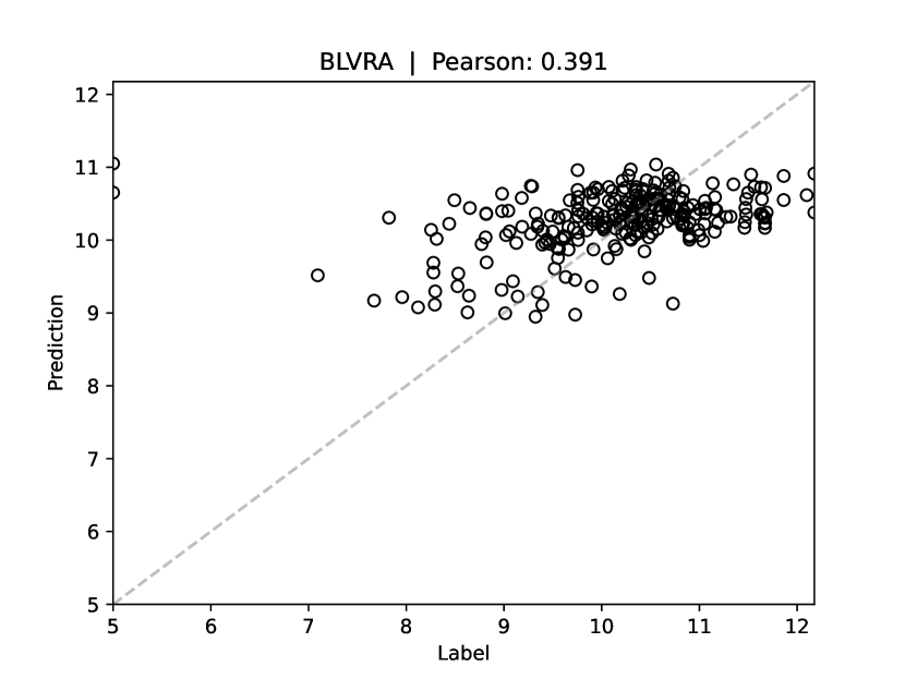
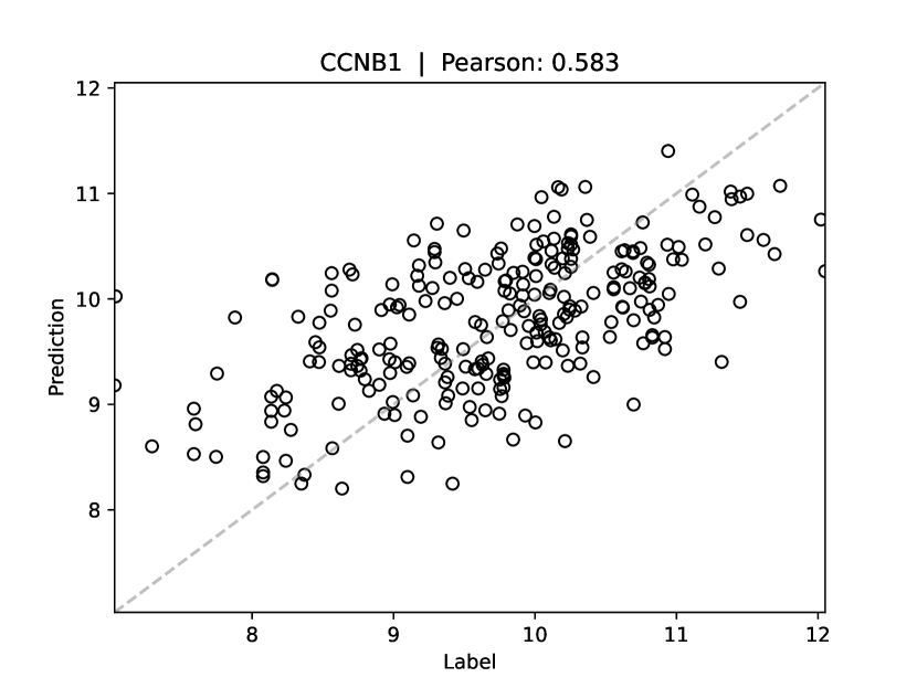
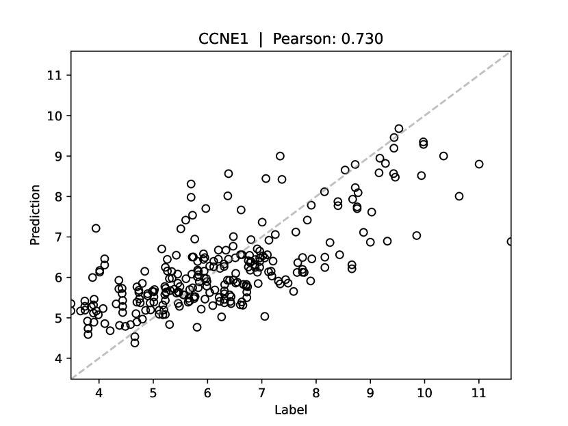
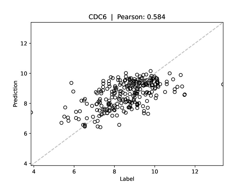
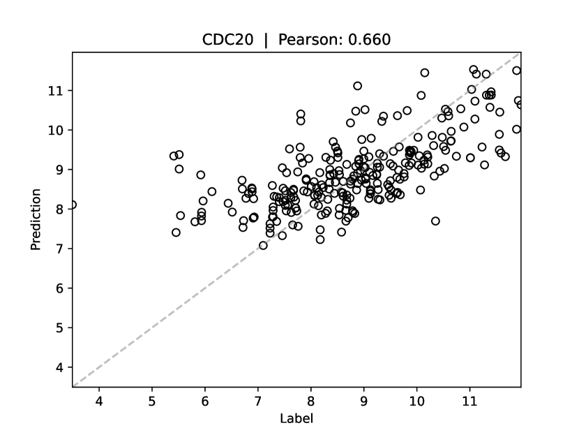
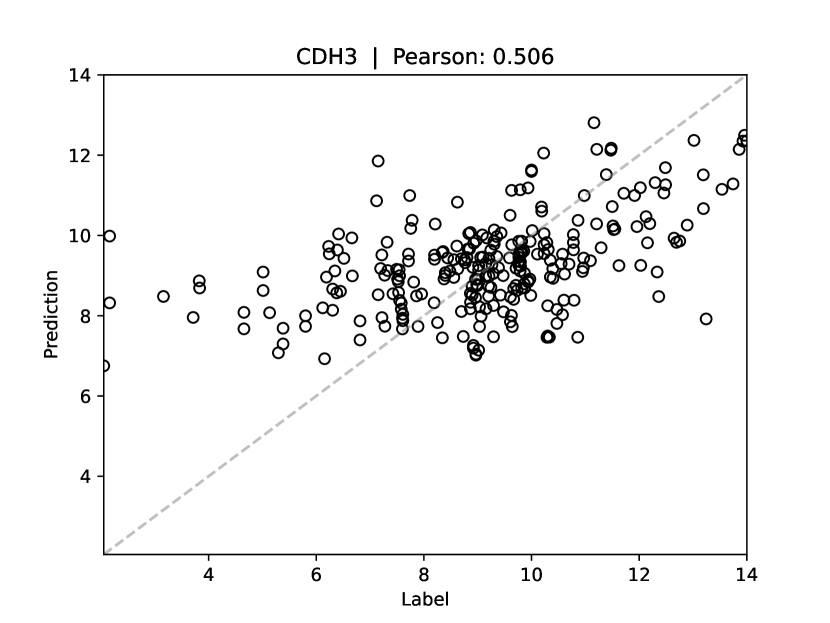
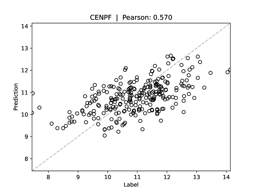
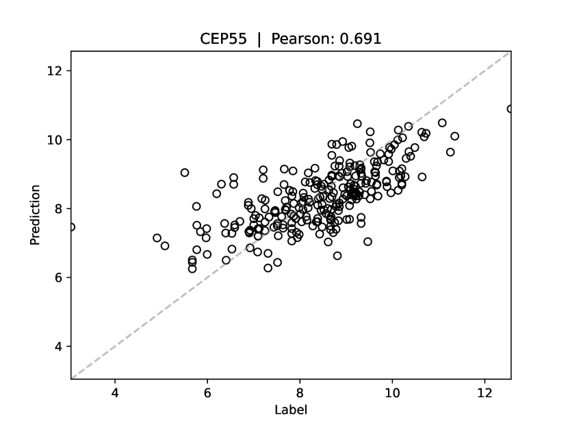
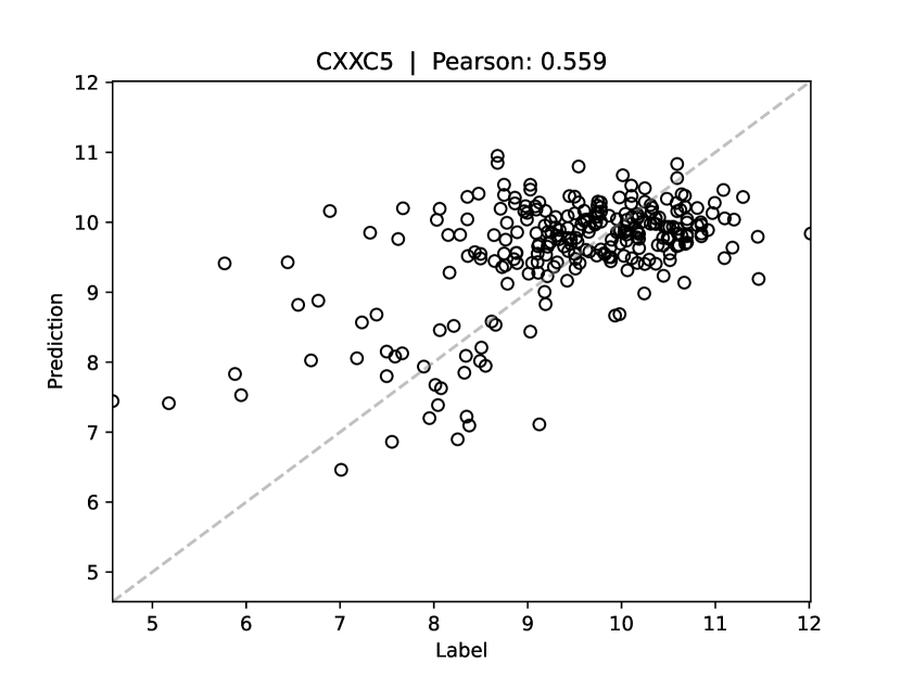
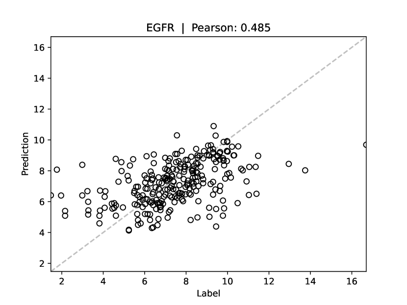
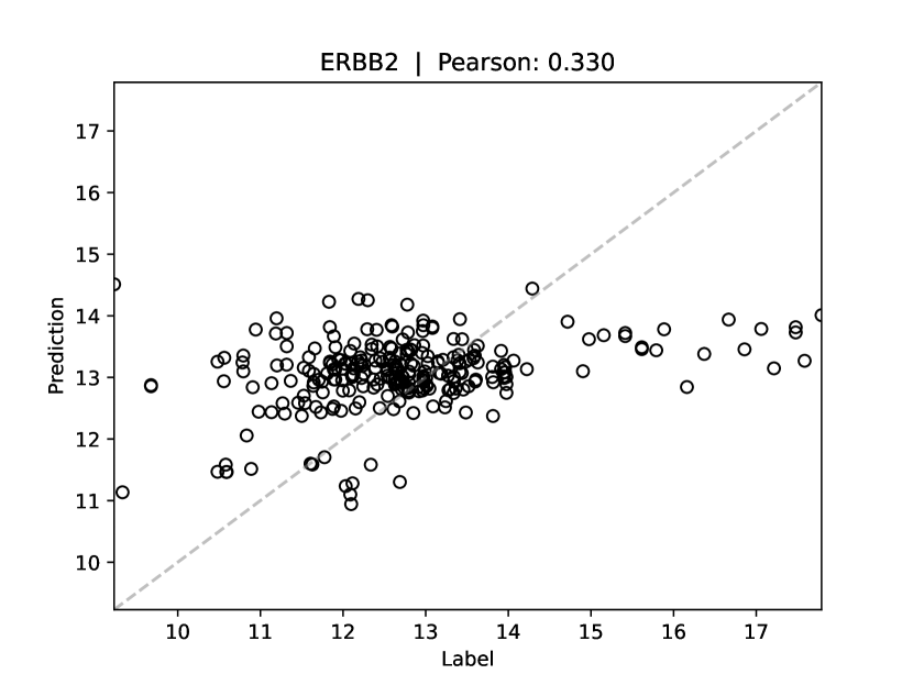
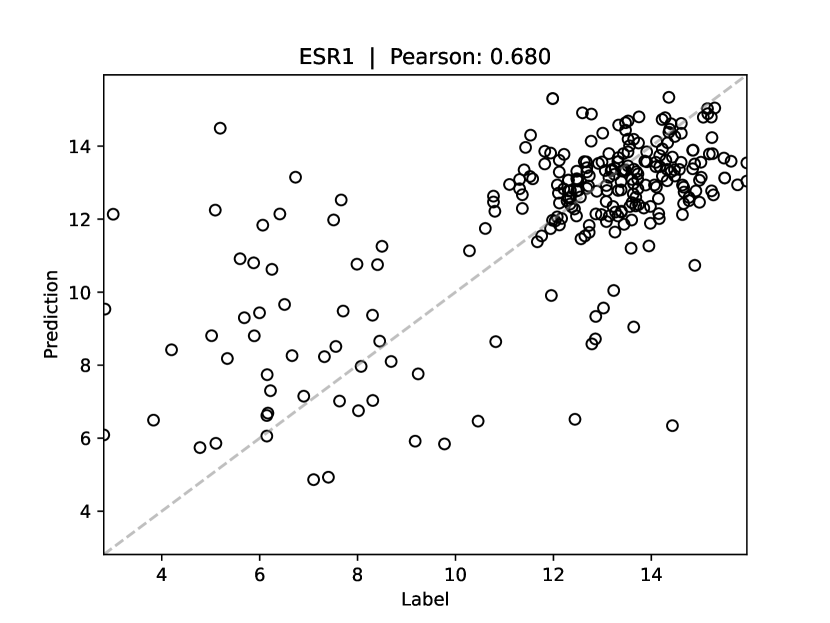
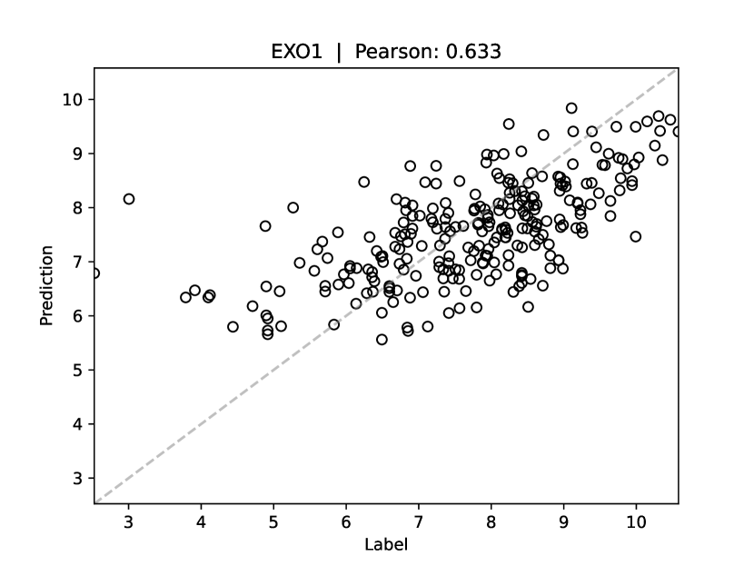
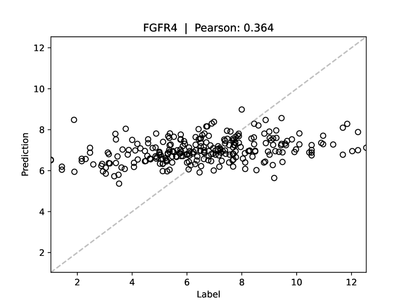
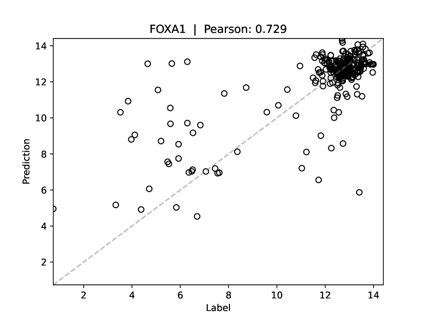
Figure S5: Correlation plots showing predicted vs ground-truth gene-expression values for PAM50 gene 6 - 20, for the UNI - Direct - ABMIL model on the TCGA-BRCA dataset, for the test split of the first cross-validation fold.

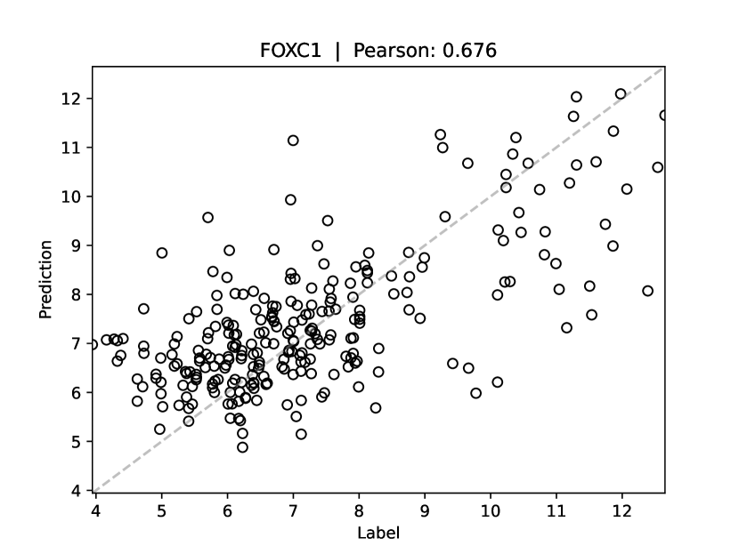
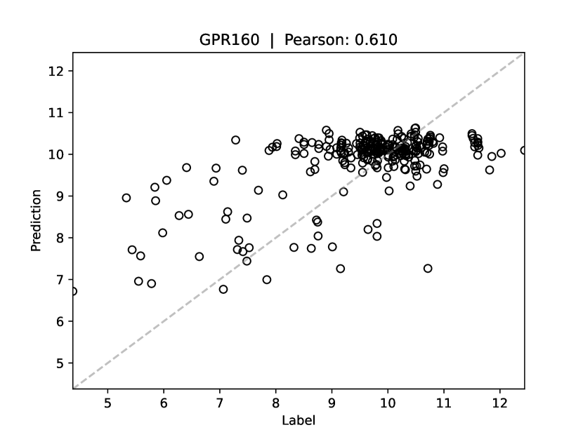
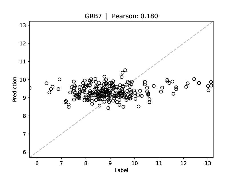
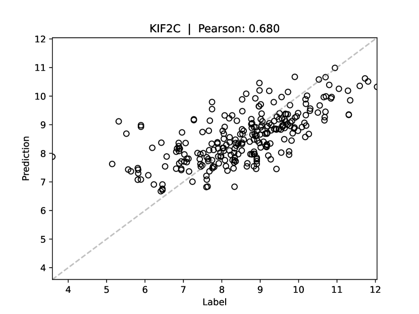
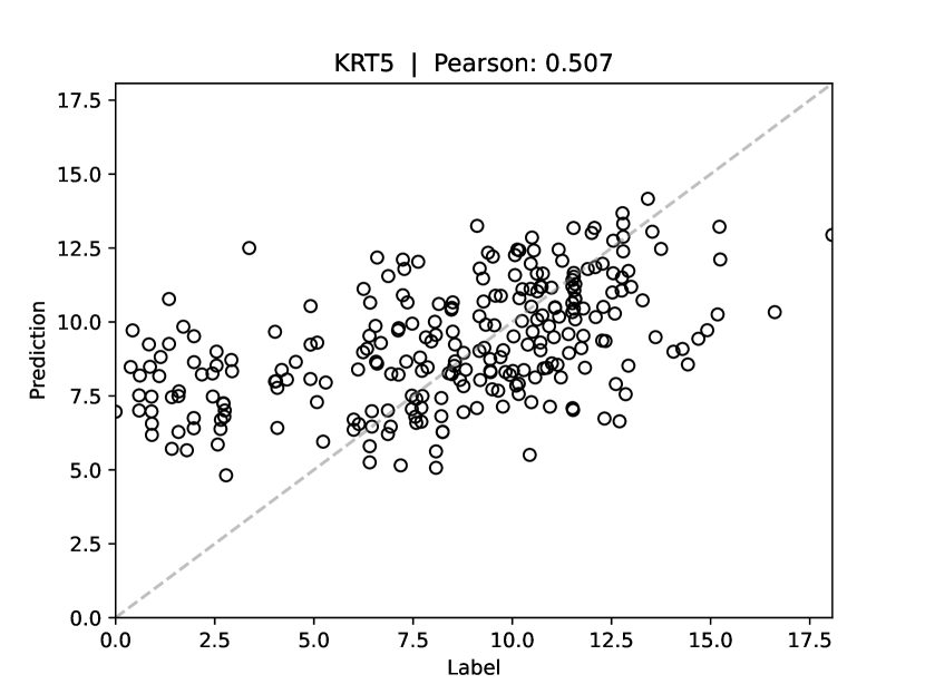
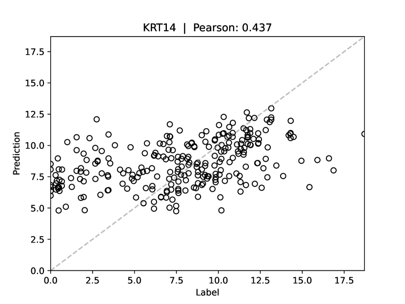
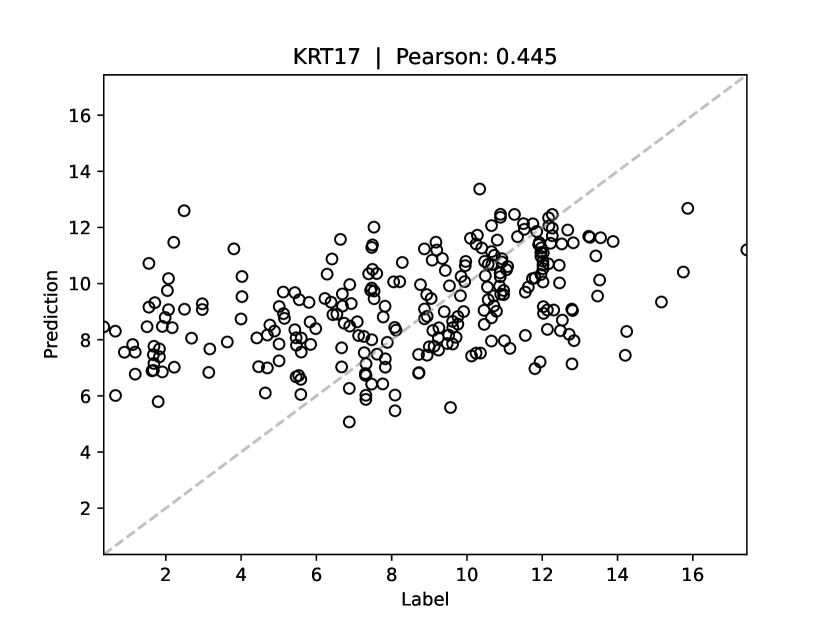
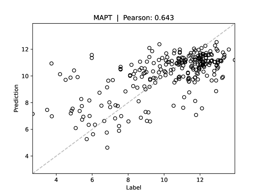
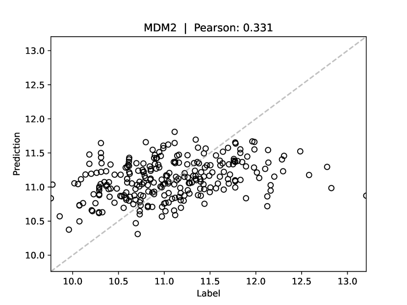
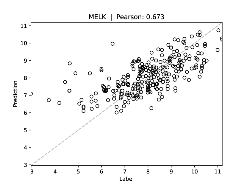
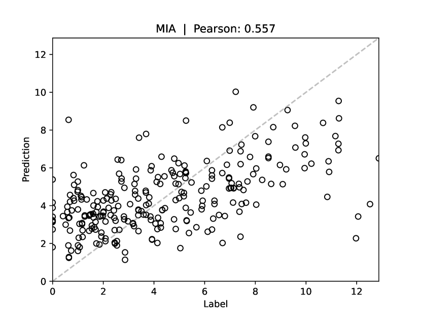
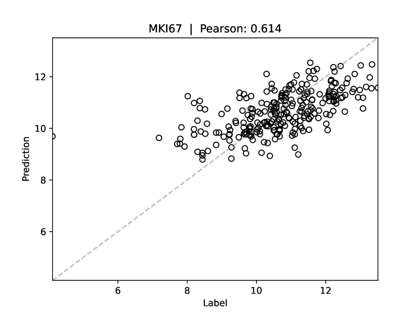
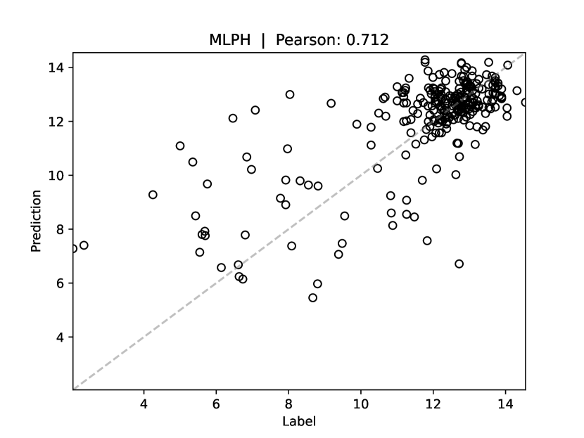
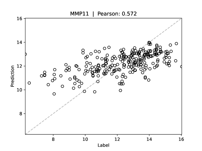
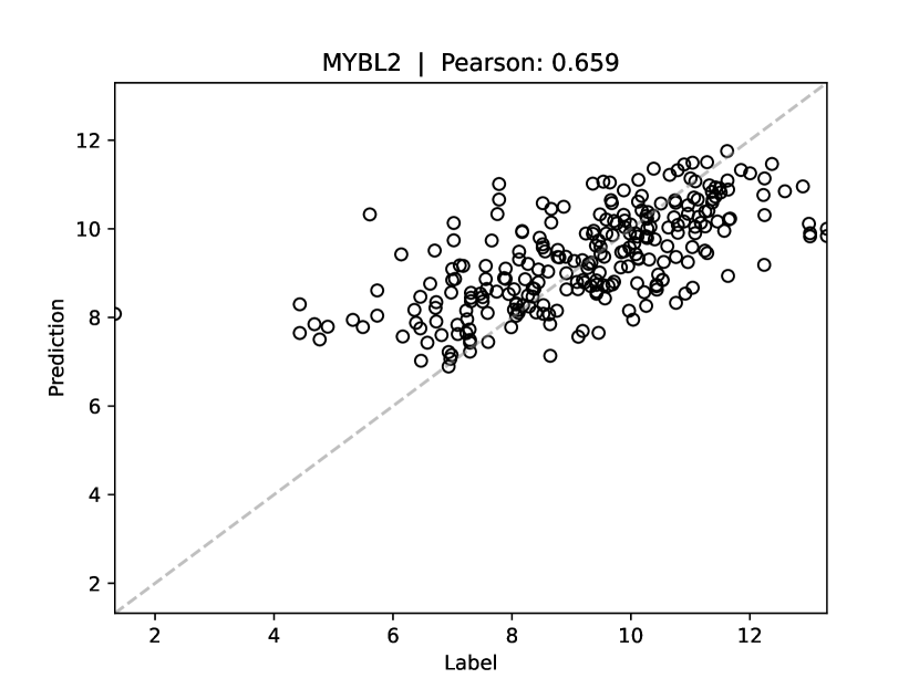
Figure S6: Correlation plots showing predicted vs ground-truth gene-expression values for PAM50 gene 21 - 35, for the UNI - Direct - ABMIL model on the TCGA-BRCA dataset, for the test split of the first cross-validation fold.

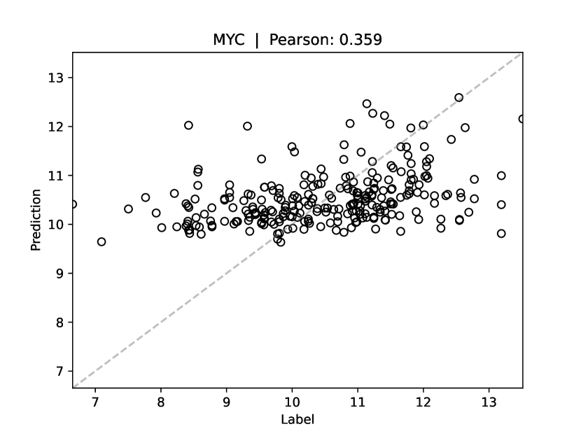
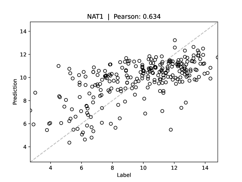
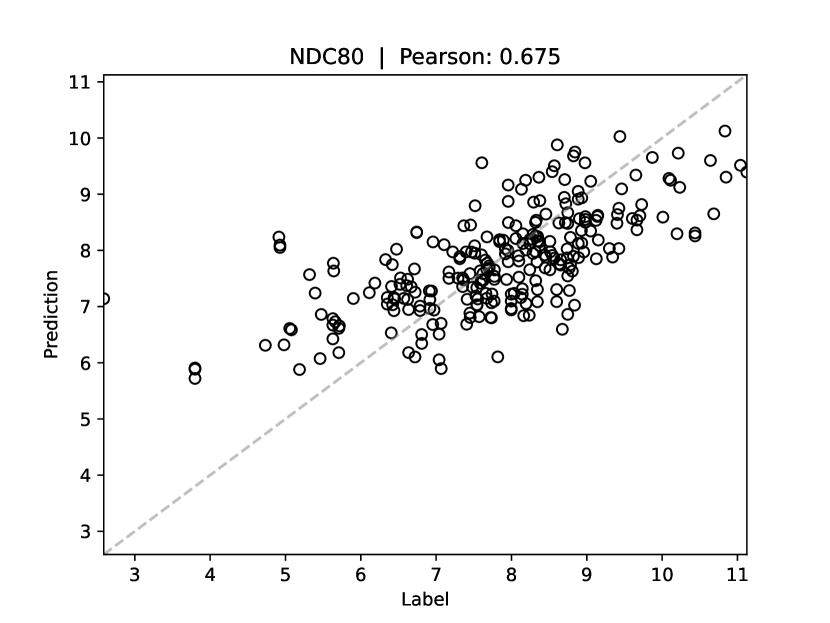
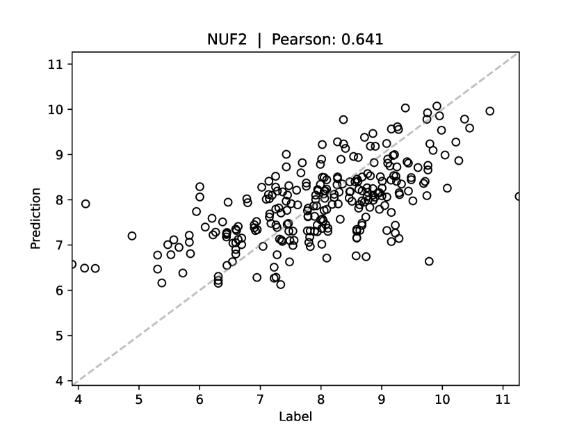
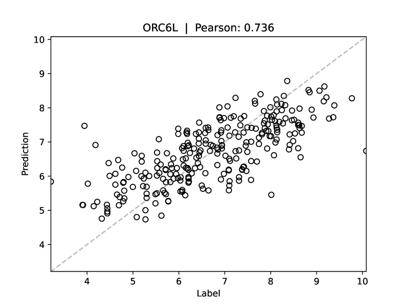
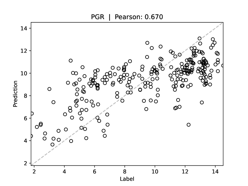
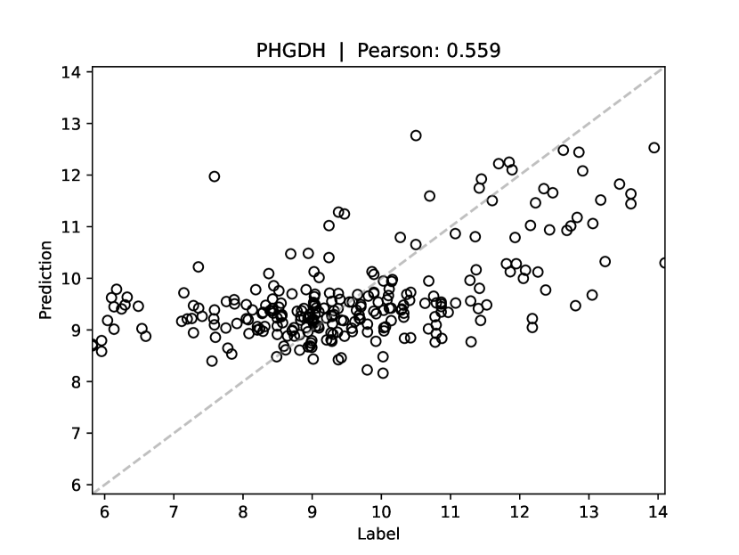
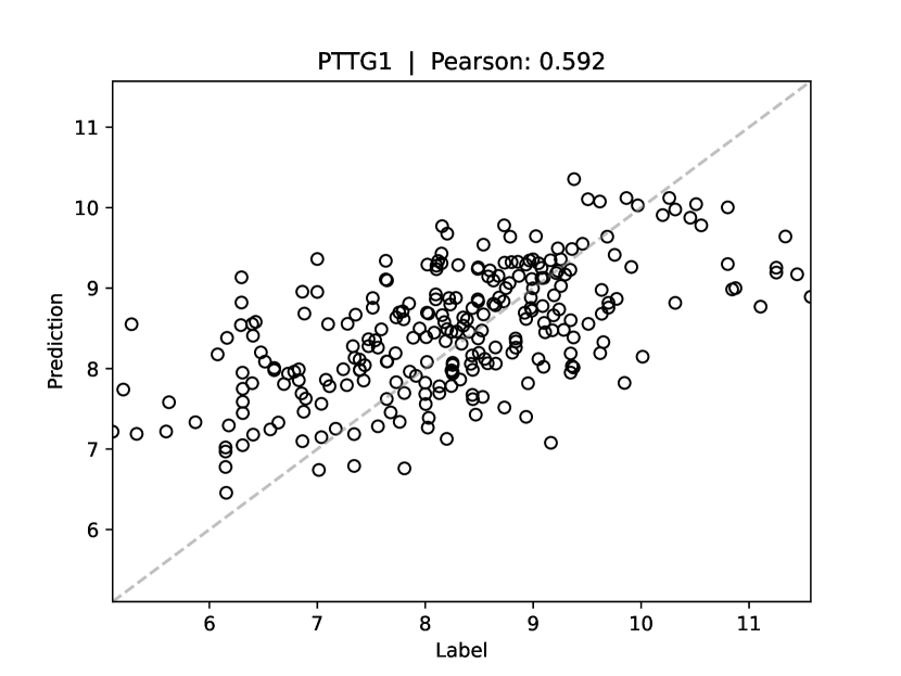
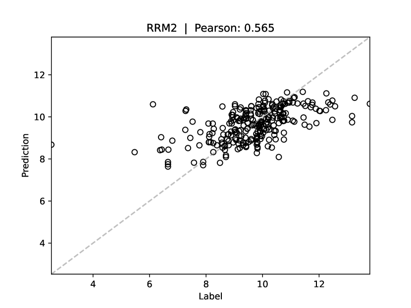
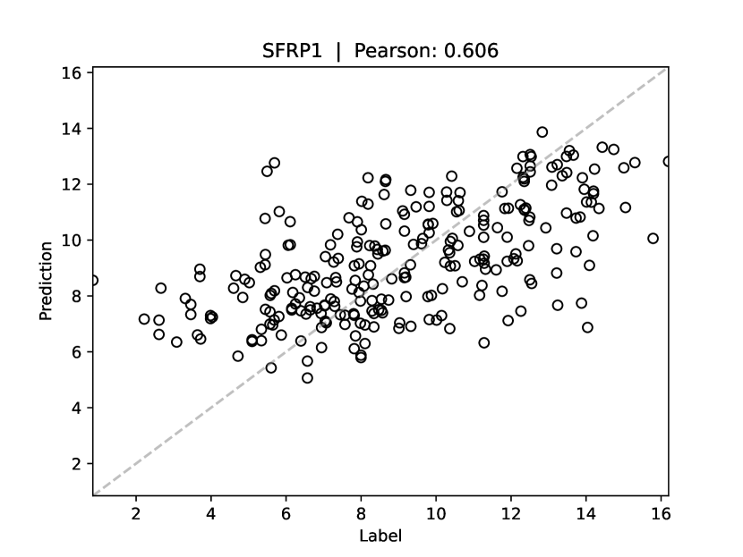
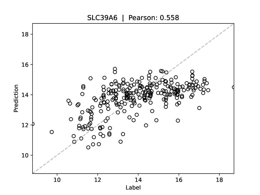
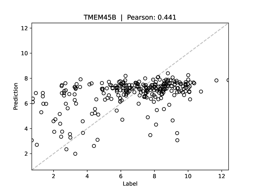
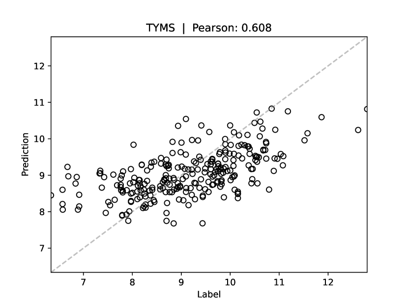
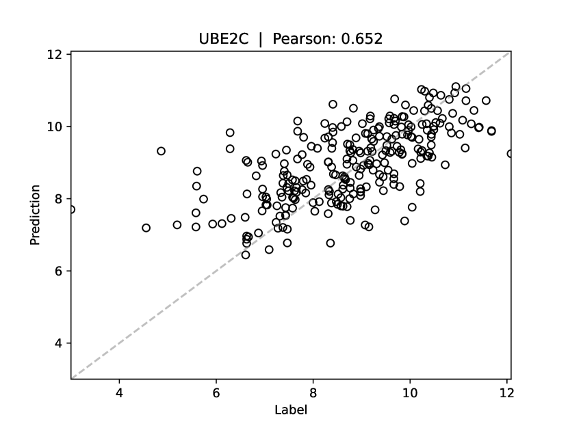
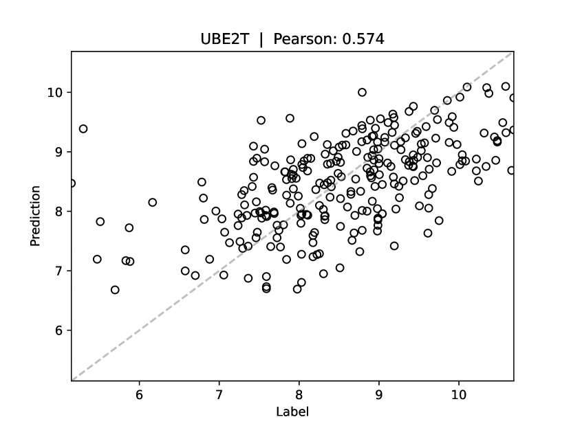
Figure S7: Correlation plots showing predicted vs ground-truth gene-expression values for PAM50 gene 36 - 50, for the UNI - Direct - ABMIL model on the TCGA-BRCA dataset, for the test split of the first cross-validation fold.

Appendix B Supplementary Tables

Table S1: Raw numerical results for Figure 1, for the TCGA-BRCA dataset. All results are mean$\pm$std over the 5 cross-validation folds, bold marks the best mean value. Higher is better for all three metrics.

	mean Pearson ($\uparrow$)	mean Pearson - top 1k genes ($\uparrow$)	# genes $\geq 0.4$ Pearson ($\uparrow$)
UNI - Direct - ABMIL	0.284$\pm$0.006	0.598$\pm$0.012	4927$\pm$357
UNI - Direct - Patch-Level	0.267$\pm$0.009	0.572$\pm$0.010	4213$\pm$353
UNI - Contrastive	0.283$\pm$0.004	0.596$\pm$0.014	4886$\pm$242
UNI - kNN	0.157$\pm$0.011	0.465$\pm$0.018	1137$\pm$247
Resnet-IN - Direct - ABMIL	0.151$\pm$0.027	0.460$\pm$0.029	1129$\pm$420
Resnet-IN - Direct - Patch-Level	0.128$\pm$0.016	0.417$\pm$0.014	574$\pm$128
Resnet-IN - Contrastive	0.217$\pm$0.029	0.515$\pm$0.042	2519$\pm$941
Resnet-IN - kNN	0.103$\pm$0.014	0.376$\pm$0.018	281$\pm$94

Table S2: Raw numerical results for Figure 1, for the TCGA-HNSC dataset. All results are mean$\pm$std over the 5 cross-validation folds, bold marks the best mean value. Higher is better for all three metrics.

	mean Pearson ($\uparrow$)	mean Pearson - top 1k genes ($\uparrow$)	# genes $\geq 0.4$ Pearson ($\uparrow$)
UNI - Direct - ABMIL	0.256$\pm$0.009	0.589$\pm$0.032	3987$\pm$765
UNI - Direct - Patch-Level	0.237$\pm$0.017	0.565$\pm$0.027	3456$\pm$837
UNI - Contrastive	0.246$\pm$0.022	0.576$\pm$0.033	3750$\pm$835
UNI - kNN	0.141$\pm$0.026	0.465$\pm$0.043	1158$\pm$463
Resnet-IN - Direct - ABMIL	0.143$\pm$0.015	0.493$\pm$0.048	1494$\pm$671
Resnet-IN - Direct - Patch-Level	0.115$\pm$0.026	0.419$\pm$0.068	767$\pm$656
Resnet-IN - Contrastive	0.183$\pm$0.022	0.533$\pm$0.047	2264$\pm$806
Resnet-IN - kNN	0.087$\pm$0.031	0.382$\pm$0.056	416$\pm$294

Table S3: Raw numerical results for Figure 1, for the TCGA-STAD dataset. All results are mean$\pm$std over the 5 cross-validation folds, bold marks the best mean value. Higher is better for all three metrics.

	mean Pearson ($\uparrow$)	mean Pearson - top 1k genes ($\uparrow$)	# genes $\geq 0.4$ Pearson ($\uparrow$)
UNI - Direct - ABMIL	0.216$\pm$0.031	0.548$\pm$0.052	3240$\pm$1342
UNI - Direct - Patch-Level	0.200$\pm$0.044	0.533$\pm$0.084	2765$\pm$1713
UNI - Contrastive	0.216$\pm$0.044	0.543$\pm$0.066	3184$\pm$1660
UNI - kNN	0.135$\pm$0.037	0.469$\pm$0.060	1328$\pm$981
Resnet-IN - Direct - ABMIL	0.110$\pm$0.038	0.431$\pm$0.101	1132$\pm$1119
Resnet-IN - Direct - Patch-Level	0.115$\pm$0.033	0.438$\pm$0.077	1068$\pm$839
Resnet-IN - Contrastive	0.124$\pm$0.035	0.444$\pm$0.069	1181$\pm$1238
Resnet-IN - kNN	0.098$\pm$0.022	0.421$\pm$0.066	794$\pm$573

Table S4: Raw numerical results for Figure 1, for the TCGA-BLCA dataset. All results are mean$\pm$std over the 5 cross-validation folds, bold marks the best mean value. Higher is better for all three metrics.

	mean Pearson ($\uparrow$)	mean Pearson - top 1k genes ($\uparrow$)	# genes $\geq 0.4$ Pearson ($\uparrow$)
UNI - Direct - ABMIL	0.253$\pm$0.029	0.600$\pm$0.037	4364$\pm$1188
UNI - Direct - Patch-Level	0.242$\pm$0.028	0.577$\pm$0.036	3822$\pm$1206
UNI - Contrastive	0.249$\pm$0.025	0.590$\pm$0.035	4183$\pm$975
UNI - kNN	0.142$\pm$0.021	0.464$\pm$0.028	1164$\pm$451
Resnet-IN - Direct - ABMIL	0.093$\pm$0.026	0.373$\pm$0.062	366$\pm$491
Resnet-IN - Direct - Patch-Level	0.087$\pm$0.024	0.389$\pm$0.060	479$\pm$373
Resnet-IN - Contrastive	0.184$\pm$0.032	0.505$\pm$0.061	2143$\pm$1077
Resnet-IN - kNN	0.088$\pm$0.016	0.380$\pm$0.049	347$\pm$289

Table S5: Results on the TCGA-BRCA dataset, when models are evaluated only on a subset of 50 genes (PAM50) with demonstrated prognostic value for breast cancer [20, 30]. All results are mean$\pm$std over the 5 cross-validation folds, bold marks the best mean value.

	mean Pearson ($\uparrow$)
UNI - Direct - ABMIL	0.562$\pm$0.020
UNI - Direct - Patch-Level	0.541$\pm$0.015
UNI - Contrastive	0.564$\pm$0.020
UNI - kNN	0.415$\pm$0.019
Resnet-IN - Direct - ABMIL	0.373$\pm$0.070
Resnet-IN - Direct - Patch-Level	0.306$\pm$0.028
Resnet-IN - Contrastive	0.449$\pm$0.046
Resnet-IN - kNN	0.267$\pm$0.026
UNI - Direct - ABMIL - Trained only on PAM50, 1 model	0.576$\pm$0.020
UNI - Direct - ABMIL - Trained only on PAM50, 2 models	0.575$\pm$0.021
UNI - Direct - ABMIL - Trained only on PAM50, 5 models	0.572$\pm$0.012
UNI - Direct - ABMIL - Trained only on PAM50, 10 models	0.569$\pm$0.016
UNI - Direct - ABMIL - Trained only on PAM50, 25 models	0.566$\pm$0.019
UNI - Direct - ABMIL - Trained only on PAM50, 50 models	0.560$\pm$0.020

Table S6: Top $20$ genes (out of the $N=20\thinspace 530$ total number of genes) with the highest regression accuracy for UNI - Direct - ABMIL, across the four TCGA datasets. All results are mean$\pm$std over the 5 cross-validation folds, sorted according to the highest mean value.

TCGA-BRCA			TCGA-HNSC			TCGA-STAD			TCGA-BLCA
Rank	Gene	Pearson ($\uparrow$)	Rank	Gene	Pearson ($\uparrow$)	Rank	Gene	Pearson ($\uparrow$)	Rank	Gene	Pearson ($\uparrow$)
1	FOXA1	0.731$\pm$0.027	1	SGEF	0.742$\pm$0.037	1	PKNOX2	0.633$\pm$0.030	1	UPK2	0.699$\pm$0.059
2	MLPH	0.726$\pm$0.048	2	LOC730101	0.726$\pm$0.055	2	JAM2	0.620$\pm$0.038	2	WARS	0.696$\pm$0.068
3	TBC1D9	0.721$\pm$0.021	3	GLS2	0.725$\pm$0.051	3	C1QTNF7	0.617$\pm$0.056	3	TOX3	0.679$\pm$0.068
4	AGR3	0.720$\pm$0.023	4	MAP7D1	0.698$\pm$0.056	4	SCN4B	0.612$\pm$0.069	4	TAP2	0.676$\pm$0.082
5	THSD4	0.713$\pm$0.023	5	KIAA1609	0.692$\pm$0.038	5	FCER1A	0.601$\pm$0.082	5	KSR2	0.670$\pm$0.070
6	CCNE1	0.711$\pm$0.032	6	ACPL2	0.691$\pm$0.025	6	CNRIP1	0.600$\pm$0.079	6	KRT6B	0.670$\pm$0.061
7	ESR1	0.709$\pm$0.018	7	MYB	0.691$\pm$0.067	7	TPX2	0.597$\pm$0.123	7	DUSP7	0.669$\pm$0.075
8	XBP1	0.701$\pm$0.025	8	C3orf58	0.687$\pm$0.016	8	DNMT3B	0.597$\pm$0.098	8	TYMP	0.667$\pm$0.054
9	ORC6L	0.701$\pm$0.035	9	KRT14	0.686$\pm$0.034	9	BHMT2	0.593$\pm$0.031	9	TRAK1	0.665$\pm$0.088
10	CENPA	0.701$\pm$0.037	10	RGS20	0.685$\pm$0.086	10	MAPK10	0.593$\pm$0.058	10	SLC30A2	0.662$\pm$0.064
11	GATA3	0.700$\pm$0.045	11	THSD1	0.684$\pm$0.035	11	GYPC	0.593$\pm$0.097	11	KRT6C	0.662$\pm$0.053
12	DNALI1	0.693$\pm$0.015	12	TUBB6	0.681$\pm$0.062	12	FHL1	0.591$\pm$0.055	12	C17orf28	0.661$\pm$0.076
13	CDC25A	0.692$\pm$0.034	13	MYO3A	0.677$\pm$0.070	13	GSTM5	0.590$\pm$0.065	13	LILRA6	0.658$\pm$0.063
14	NOSTRIN	0.691$\pm$0.045	14	MT2A	0.671$\pm$0.058	14	TCEAL7	0.588$\pm$0.116	14	PDCD1LG2	0.657$\pm$0.040
15	SCUBE2	0.690$\pm$0.014	15	SLC31A2	0.670$\pm$0.059	15	ABCA8	0.584$\pm$0.043	15	KLHDC7A	0.654$\pm$0.082
16	SPDEF	0.690$\pm$0.043	16	MRAP2	0.668$\pm$0.027	16	FAM107A	0.581$\pm$0.059	16	SLC9A2	0.653$\pm$0.069
17	PSAT1	0.688$\pm$0.027	17	SP110	0.665$\pm$0.051	17	FXYD1	0.580$\pm$0.114	17	BHMT	0.649$\pm$0.058
18	CENPN	0.688$\pm$0.027	18	TMEM116	0.662$\pm$0.050	18	HJURP	0.579$\pm$0.092	18	FAM190A	0.647$\pm$0.037
19	C6orf97	0.687$\pm$0.034	19	SAMD12	0.661$\pm$0.023	19	FGF7	0.577$\pm$0.097	19	LOC100188947	0.647$\pm$0.083
20	SLC44A4	0.686$\pm$0.035	20	CAV1	0.661$\pm$0.044	20	TOP2A	0.577$\pm$0.117	20	FCGR3A	0.645$\pm$0.049

Table S7: Top $20$ genes (out of the $N=20\thinspace 530$ total number of genes) with the highest regression accuracy for UNI - Contrastive, across the four TCGA datasets. All results are mean$\pm$std over the 5 cross-validation folds, sorted according to the highest mean value. Compared to the results for the UNI - Direct - ABMIL model in Table S6, $17$ of the top $20$ genes are shared on TCGA-BRCA, $14$/$20$ genes on TCGA-HNSC, $13$/$20$ genes on TCGA-STAD, and $14$/$20$ genes on TCGA-BLCA.

TCGA-BRCA			TCGA-HNSC			TCGA-STAD			TCGA-BLCA
Rank	Gene	Pearson ($\uparrow$)	Rank	Gene	Pearson ($\uparrow$)	Rank	Gene	Pearson ($\uparrow$)	Rank	Gene	Pearson ($\uparrow$)
1	FOXA1	0.731$\pm$0.030	1	LOC730101	0.712$\pm$0.075	1	SCN4B	0.616$\pm$0.105	1	UPK2	0.695$\pm$0.040
2	AGR3	0.725$\pm$0.046	2	GLS2	0.696$\pm$0.064	2	C1QTNF7	0.616$\pm$0.073	2	WARS	0.691$\pm$0.073
3	MLPH	0.722$\pm$0.049	3	SGEF	0.691$\pm$0.019	3	PKNOX2	0.610$\pm$0.081	3	KSR2	0.686$\pm$0.065
4	ESR1	0.719$\pm$0.025	4	MAP7D1	0.678$\pm$0.077	4	NEGR1	0.599$\pm$0.080	4	C17orf28	0.677$\pm$0.046
5	THSD4	0.717$\pm$0.025	5	CAV1	0.676$\pm$0.050	5	JAM2	0.597$\pm$0.069	5	TAP2	0.668$\pm$0.082
6	TBC1D9	0.712$\pm$0.043	6	MYB	0.672$\pm$0.083	6	RBMS3	0.591$\pm$0.103	6	KLHDC7A	0.663$\pm$0.046
7	CCNE1	0.709$\pm$0.027	7	KIAA1609	0.672$\pm$0.028	7	BOC	0.587$\pm$0.085	7	TOX3	0.661$\pm$0.055
8	C6orf97	0.697$\pm$0.042	8	ACPL2	0.664$\pm$0.043	8	JAM3	0.586$\pm$0.071	8	DUSP7	0.661$\pm$0.063
9	DEGS2	0.696$\pm$0.036	9	SLC31A2	0.662$\pm$0.050	9	CCNA2	0.585$\pm$0.098	9	SLC9A2	0.657$\pm$0.082
10	CENPA	0.694$\pm$0.034	10	THSD1	0.660$\pm$0.049	10	FHL1	0.585$\pm$0.070	10	SLC30A2	0.656$\pm$0.044
11	XBP1	0.694$\pm$0.036	11	RGS20	0.657$\pm$0.093	11	MAPK10	0.584$\pm$0.083	11	PDCD1LG2	0.654$\pm$0.042
12	SCUBE2	0.694$\pm$0.015	12	KRT14	0.655$\pm$0.042	12	HJURP	0.583$\pm$0.087	12	TYMP	0.653$\pm$0.078
13	ORC6L	0.692$\pm$0.042	13	TNFRSF12A	0.654$\pm$0.081	13	FCER1A	0.582$\pm$0.078	13	TRAK1	0.647$\pm$0.055
14	CENPN	0.692$\pm$0.037	14	SP110	0.651$\pm$0.055	14	MFAP4	0.582$\pm$0.067	14	RAB15	0.646$\pm$0.089
15	GATA3	0.689$\pm$0.054	15	C3orf58	0.648$\pm$0.014	15	BHMT2	0.581$\pm$0.077	15	SNX31	0.646$\pm$0.070
16	SLC44A4	0.688$\pm$0.051	16	RPS6KA4	0.644$\pm$0.071	16	FXYD1	0.580$\pm$0.102	16	RHOU	0.645$\pm$0.093
17	NOSTRIN	0.687$\pm$0.038	17	FHOD1	0.643$\pm$0.064	17	DNMT3B	0.579$\pm$0.075	17	UPK3A	0.644$\pm$0.045
18	LRRC17	0.687$\pm$0.039	18	SBK1	0.640$\pm$0.097	18	CNRIP1	0.578$\pm$0.083	18	KRT6B	0.641$\pm$0.078
19	CA12	0.687$\pm$0.030	19	FLRT3	0.636$\pm$0.060	19	FAT4	0.577$\pm$0.099	19	SERPINB1	0.641$\pm$0.075
20	SPDEF	0.686$\pm$0.044	20	KRT6C	0.636$\pm$0.061	20	TCEAL7	0.576$\pm$0.116	20	UPK1A	0.639$\pm$0.078

Table S8: Regression accuracy for each of the individual PAM50 genes on the TCGA-BRCA dataset, for the UNI - Direct - ABMIL model. All results are mean$\pm$std over the 5 cross-validation folds, sorted according to the highest mean value.

Rank	Gene	Pearson ($\uparrow$)	Rank	Gene	Pearson ($\uparrow$)	Rank	Gene	Pearson ($\uparrow$)	Rank	Gene	Pearson ($\uparrow$)
1	FOXA1	0.731$\pm$0.027	14	BIRC5	0.649$\pm$0.040	27	ANLN	0.576$\pm$0.063	40	MMP11	0.469$\pm$0.058
2	MLPH	0.726$\pm$0.048	15	NAT1	0.635$\pm$0.042	28	CDC6	0.571$\pm$0.053	41	KRT17	0.465$\pm$0.036
3	CCNE1	0.711$\pm$0.032	16	GPR160	0.634$\pm$0.054	29	MKI67	0.569$\pm$0.053	42	TMEM45B	0.460$\pm$0.045
4	ESR1	0.709$\pm$0.018	17	MAPT	0.624$\pm$0.056	30	CXXC5	0.568$\pm$0.039	43	MYC	0.439$\pm$0.047
5	ORC6L	0.701$\pm$0.035	18	PGR	0.619$\pm$0.034	31	TYMS	0.558$\pm$0.044	44	KRT14	0.417$\pm$0.040
6	CDC20	0.682$\pm$0.019	19	PTTG1	0.616$\pm$0.023	32	SFRP1	0.555$\pm$0.046	45	BAG1	0.374$\pm$0.057
7	KIF2C	0.674$\pm$0.032	20	BCL2	0.614$\pm$0.063	33	PHGDH	0.552$\pm$0.034	46	BLVRA	0.370$\pm$0.044
8	MYBL2	0.673$\pm$0.025	21	EXO1	0.610$\pm$0.032	34	MIA	0.542$\pm$0.052	47	ERBB2	0.360$\pm$0.065
9	MELK	0.661$\pm$0.035	22	SLC39A6	0.607$\pm$0.034	35	CDH3	0.537$\pm$0.042	48	MDM2	0.344$\pm$0.039
10	FOXC1	0.655$\pm$0.037	23	CCNB1	0.600$\pm$0.060	36	CENPF	0.524$\pm$0.046	49	FGFR4	0.318$\pm$0.041
11	CEP55	0.654$\pm$0.052	24	NUF2	0.600$\pm$0.028	37	EGFR	0.513$\pm$0.039	50	GRB7	0.181$\pm$0.107
12	NDC80	0.654$\pm$0.049	25	RRM2	0.597$\pm$0.039	38	ACTR3B	0.493$\pm$0.080
13	UBE2C	0.650$\pm$0.029	26	UBE2T	0.593$\pm$0.041	39	KRT5	0.477$\pm$0.037

Table S9: Regression accuracy for each of the individual PAM50 genes on the TCGA-BRCA dataset, for the UNI - Contrastive model. All results are mean$\pm$std over the 5 cross-validation folds, sorted according to the highest mean value.

Rank	Gene	Pearson ($\uparrow$)	Rank	Gene	Pearson ($\uparrow$)	Rank	Gene	Pearson ($\uparrow$)	Rank	Gene	Pearson ($\uparrow$)
1	FOXA1	0.731$\pm$0.030	14	NDC80	0.647$\pm$0.061	27	UBE2T	0.576$\pm$0.040	40	KRT17	0.484$\pm$0.045
2	MLPH	0.722$\pm$0.049	15	NAT1	0.639$\pm$0.038	28	SFRP1	0.574$\pm$0.027	41	TMEM45B	0.472$\pm$0.046
3	ESR1	0.719$\pm$0.025	16	MAPT	0.632$\pm$0.054	29	ANLN	0.572$\pm$0.041	42	MMP11	0.468$\pm$0.060
4	CCNE1	0.709$\pm$0.027	17	GPR160	0.628$\pm$0.055	30	CDC6	0.569$\pm$0.043	43	MYC	0.443$\pm$0.038
5	ORC6L	0.692$\pm$0.042	18	BCL2	0.627$\pm$0.058	31	MKI67	0.561$\pm$0.027	44	KRT14	0.440$\pm$0.043
6	CDC20	0.676$\pm$0.032	19	PGR	0.613$\pm$0.038	32	CDH3	0.559$\pm$0.016	45	ERBB2	0.392$\pm$0.046
7	KIF2C	0.661$\pm$0.036	20	PTTG1	0.612$\pm$0.031	33	PHGDH	0.550$\pm$0.041	46	BAG1	0.368$\pm$0.059
8	MYBL2	0.659$\pm$0.033	21	SLC39A6	0.601$\pm$0.020	34	TYMS	0.547$\pm$0.054	47	BLVRA	0.366$\pm$0.068
9	FOXC1	0.656$\pm$0.035	22	RRM2	0.593$\pm$0.031	35	MIA	0.542$\pm$0.034	48	MDM2	0.354$\pm$0.026
10	BIRC5	0.655$\pm$0.038	23	EXO1	0.589$\pm$0.029	36	EGFR	0.538$\pm$0.034	49	FGFR4	0.333$\pm$0.054
11	MELK	0.652$\pm$0.035	24	CXXC5	0.585$\pm$0.054	37	KRT5	0.494$\pm$0.028	50	GRB7	0.247$\pm$0.081
12	CEP55	0.650$\pm$0.052	25	CCNB1	0.580$\pm$0.058	38	CENPF	0.492$\pm$0.041
13	UBE2C	0.647$\pm$0.036	26	NUF2	0.578$\pm$0.021	39	ACTR3B	0.491$\pm$0.089

References

- Chen et al. [2024] Richard J Chen, Tong Ding, Ming Y Lu, Drew FK Williamson, Guillaume Jaume, Andrew H Song, Bowen Chen, Andrew Zhang, Daniel Shao, Muhammad Shaban, et al. Towards a general-purpose foundation model for computational pathology. Nature Medicine, 30(3):850–862, 2024.
- Chen et al. [2020] Ting Chen, Simon Kornblith, Mohammad Norouzi, and Geoffrey Hinton. A simple framework for contrastive learning of visual representations. In International Conference on Machine Learning (ICML), pages 1597–1607, 2020.
- Dosovitskiy et al. [2021] Alexey Dosovitskiy, Lucas Beyer, Alexander Kolesnikov, Dirk Weissenborn, Xiaohua Zhai, Thomas Unterthiner, Mostafa Dehghani, Matthias Minderer, Georg Heigold, Sylvain Gelly, Jakob Uszkoreit, and Neil Houlsby. An image is worth 16x16 words: Transformers for image recognition at scale. In International Conference on Learning Representations (ICLR), 2021.
- Garrido et al. [2023] Quentin Garrido, Randall Balestriero, Laurent Najman, and Yann Lecun. Rankme: Assessing the downstream performance of pretrained self-supervised representations by their rank. In International Conference on Machine Learning (ICML), pages 10929–10974, 2023.
- Goldman et al. [2020] Mary J Goldman, Brian Craft, Mim Hastie, Kristupas Repečka, Fran McDade, Akhil Kamath, Ayan Banerjee, Yunhai Luo, Dave Rogers, Angela N Brooks, et al. Visualizing and interpreting cancer genomics data via the xena platform. Nature Biotechnology, 38(6):675–678, 2020.
- Gustafsson et al. [2020] Fredrik K Gustafsson, Martin Danelljan, Goutam Bhat, and Thomas B Schön. Energy-based models for deep probabilistic regression. In Proceedings of the European Conference on Computer Vision (ECCV), pages 325–343, 2020.
- He et al. [2016] Kaiming He, Xiangyu Zhang, Shaoqing Ren, and Jian Sun. Deep residual learning for image recognition. In Proceedings of the IEEE Conference on Computer Vision and Pattern Recognition (CVPR), pages 770–778, 2016.
- Hoang et al. [2024] Danh-Tai Hoang, Gal Dinstag, Eldad D Shulman, Leandro C Hermida, Doreen S Ben-Zvi, Efrat Elis, Katherine Caley, Stephen-John Sammut, Sanju Sinha, Neelam Sinha, et al. A deep-learning framework to predict cancer treatment response from histopathology images through imputed transcriptomics. Nature Cancer, pages 1–13, 2024.
- Howard et al. [2021] Frederick M Howard, James Dolezal, Sara Kochanny, Jefree Schulte, Heather Chen, Lara Heij, Dezheng Huo, Rita Nanda, Olufunmilayo I Olopade, Jakob N Kather, et al. The impact of site-specific digital histology signatures on deep learning model accuracy and bias. Nature Communications, 12(1):4423, 2021.
- Ilse et al. [2018] Maximilian Ilse, Jakub Tomczak, and Max Welling. Attention-based deep multiple instance learning. In International Conference on Machine Learning (ICML), pages 2127–2136, 2018.
- Jaume et al. [2024] Guillaume Jaume, Lukas Oldenburg, Anurag Vaidya, Richard J Chen, Drew FK Williamson, Thomas Peeters, Andrew H Song, and Faisal Mahmood. Transcriptomics-guided slide representation learning in computational pathology. In Proceedings of the IEEE/CVF Conference on Computer Vision and Pattern Recognition (CVPR), pages 9632–9644, 2024.
- Laleh et al. [2022] Narmin Ghaffari Laleh, Hannah Sophie Muti, Chiara Maria Lavinia Loeffler, Amelie Echle, Oliver Lester Saldanha, Faisal Mahmood, Ming Y Lu, Christian Trautwein, Rupert Langer, Bastian Dislich, et al. Benchmarking weakly-supervised deep learning pipelines for whole slide classification in computational pathology. Medical Image Analysis, 79, 2022.
- Lathuilière et al. [2019] Stéphane Lathuilière, Pablo Mesejo, Xavier Alameda-Pineda, and Radu Horaud. A comprehensive analysis of deep regression. IEEE Transactions on Pattern Analysis and Machine Intelligence (TPAMI), 2019.
- Loshchilov and Hutter [2019] Ilya Loshchilov and Frank Hutter. Decoupled weight decay regularization. In International Conference on Learning Representations (ICLR), 2019.
- Lu et al. [2021] Ming Y Lu, Drew FK Williamson, Tiffany Y Chen, Richard J Chen, Matteo Barbieri, and Faisal Mahmood. Data-efficient and weakly supervised computational pathology on whole-slide images. Nature Biomedical Engineering, 5(6):555–570, 2021.
- Lu et al. [2024] Ming Y Lu, Bowen Chen, Drew FK Williamson, Richard J Chen, Ivy Liang, Tong Ding, Guillaume Jaume, Igor Odintsov, Long Phi Le, Georg Gerber, et al. A visual-language foundation model for computational pathology. Nature Medicine, 30:863–874, 2024.
- McDermott et al. [2011] Ultan McDermott, James R Downing, and Michael R Stratton. Genomics and the continuum of cancer care. New England Journal of Medicine, 364(4):340–350, 2011.
- Min et al. [2024] Wenwen Min, Zhiceng Shi, Jun Zhang, Jun Wan, and Changmiao Wang. Multimodal contrastive learning for spatial gene expression prediction using histology images. arXiv preprint arXiv:2407.08216, 2024.
- Mondol et al. [2023] Raktim Kumar Mondol, Ewan KA Millar, Peter H Graham, Lois Browne, Arcot Sowmya, and Erik Meijering. hist2rna: an efficient deep learning architecture to predict gene expression from breast cancer histopathology images. Cancers, 15(9):2569, 2023.
- Nielsen et al. [2010] Torsten O Nielsen, Joel S Parker, Samuel Leung, David Voduc, Mark Ebbert, Tammi Vickery, Sherri R Davies, Jacqueline Snider, Inge J Stijleman, Jerry Reed, et al. A comparison of pam50 intrinsic subtyping with immunohistochemistry and clinical prognostic factors in tamoxifen-treated estrogen receptor–positive breast cancer. Clinical Cancer Research, 16(21):5222–5232, 2010.
- Oquab et al. [2024] Maxime Oquab, Timothée Darcet, Théo Moutakanni, Huy V. Vo, Marc Szafraniec, Vasil Khalidov, Pierre Fernandez, Daniel HAZIZA, Francisco Massa, Alaaeldin El-Nouby, Mido Assran, Nicolas Ballas, Wojciech Galuba, Russell Howes, Po-Yao Huang, Shang-Wen Li, Ishan Misra, Michael Rabbat, Vasu Sharma, Gabriel Synnaeve, Hu Xu, Herve Jegou, Julien Mairal, Patrick Labatut, Armand Joulin, and Piotr Bojanowski. DINOv2: Learning robust visual features without supervision. Transactions on Machine Learning Research (TMLR), 2024.
- Pedregosa et al. [2011] F. Pedregosa, G. Varoquaux, A. Gramfort, V. Michel, B. Thirion, O. Grisel, M. Blondel, P. Prettenhofer, R. Weiss, V. Dubourg, J. Vanderplas, A. Passos, D. Cournapeau, M. Brucher, M. Perrot, and E. Duchesnay. Scikit-learn: Machine learning in Python. Journal of Machine Learning Research (JMLR), 12:2825–2830, 2011.
- Radford et al. [2021] Alec Radford, Jong Wook Kim, Chris Hallacy, Aditya Ramesh, Gabriel Goh, Sandhini Agarwal, Girish Sastry, Amanda Askell, Pamela Mishkin, Jack Clark, et al. Learning transferable visual models from natural language supervision. In International Conference on Machine Learning (ICML), pages 8748–8763, 2021.
- Ren et al. [2018] Shancheng Ren, Gong-Hong Wei, Dongbing Liu, Liguo Wang, Yong Hou, Shida Zhu, Lihua Peng, Qin Zhang, Yanbing Cheng, Hong Su, et al. Whole-genome and transcriptome sequencing of prostate cancer identify new genetic alterations driving disease progression. European urology, 73(3):322–339, 2018.
- Russakovsky et al. [2015] Olga Russakovsky, Jia Deng, Hao Su, Jonathan Krause, Sanjeev Satheesh, Sean Ma, Zhiheng Huang, Andrej Karpathy, Aditya Khosla, Michael Bernstein, et al. Imagenet large scale visual recognition challenge. International Journal of Computer Vision (IJCV), 115:211–252, 2015.
- Schmauch et al. [2020] Benoît Schmauch, Alberto Romagnoni, Elodie Pronier, Charlie Saillard, Pascale Maillé, Julien Calderaro, Aurélie Kamoun, Meriem Sefta, Sylvain Toldo, Mikhail Zaslavskiy, et al. A deep learning model to predict rna-seq expression of tumours from whole slide images. Nature Communications, 11(1):3877, 2020.
- Van De Vijver et al. [2002] Marc J Van De Vijver, Yudong D He, Laura J Van’t Veer, Hongyue Dai, Augustinus AM Hart, Dorien W Voskuil, George J Schreiber, Johannes L Peterse, Chris Roberts, Matthew J Marton, et al. A gene-expression signature as a predictor of survival in breast cancer. New England Journal of Medicine, 347(25):1999–2009, 2002.
- Van’t Veer et al. [2002] Laura J Van’t Veer, Hongyue Dai, Marc J Van De Vijver, Yudong D He, Augustinus AM Hart, Mao Mao, Hans L Peterse, Karin Van Der Kooy, Matthew J Marton, Anke T Witteveen, et al. Gene expression profiling predicts clinical outcome of breast cancer. Nature, 415(6871):530–536, 2002.
- Vorontsov et al. [2024] Eugene Vorontsov, Alican Bozkurt, Adam Casson, George Shaikovski, Michal Zelechowski, Kristen Severson, Eric Zimmermann, James Hall, Neil Tenenholtz, Nicolo Fusi, et al. A foundation model for clinical-grade computational pathology and rare cancers detection. Nature Medicine, pages 1–12, 2024.
- Wallden et al. [2015] Brett Wallden, James Storhoff, Torsten Nielsen, Naeem Dowidar, Carl Schaper, Sean Ferree, Shuzhen Liu, Samuel Leung, Gary Geiss, Jacqueline Snider, et al. Development and verification of the pam50-based prosigna breast cancer gene signature assay. BMC Medical Genomics, 8:1–14, 2015.
- Wang et al. [2021] Yinxi Wang, Kimmo Kartasalo, Philippe Weitz, Balazs Acs, Masi Valkonen, Christer Larsson, Pekka Ruusuvuori, Johan Hartman, and Mattias Rantalainen. Predicting molecular phenotypes from histopathology images: a transcriptome-wide expression–morphology analysis in breast cancer. Cancer research, 81(19):5115–5126, 2021.
- Weitz et al. [2022] Philippe Weitz, Yinxi Wang, Kimmo Kartasalo, Lars Egevad, Johan Lindberg, Henrik Grönberg, Martin Eklund, and Mattias Rantalainen. Transcriptome-wide prediction of prostate cancer gene expression from histopathology images using co-expression-based convolutional neural networks. Bioinformatics, 38(13):3462–3469, 2022.
- Xie et al. [2023] Ronald Xie, Kuan Pang, Sai Chung, Catia Perciani, Sonya MacParland, Bo Wang, and Gary Bader. Spatially resolved gene expression prediction from histology images via bi-modal contrastive learning. Advances in Neural Information Processing Systems (NeurIPS), 2023.
- Xu et al. [2024] Hanwen Xu, Naoto Usuyama, Jaspreet Bagga, Sheng Zhang, Rajesh Rao, Tristan Naumann, Cliff Wong, Zelalem Gero, Javier González, Yu Gu, et al. A whole-slide foundation model for digital pathology from real-world data. Nature, pages 1–8, 2024.