Anisotropic Spherical Solutions in Rastall Gravity by Gravitational Decoupling

Abstract

In this paper, we extend the Finch-Skea isotropic ansatz representing a self-gravitating interior to two anisotropic spherical solutions within the context of Rastall gravity. For this purpose, we use a newly developed technique, named as gravitational decoupling approach through the minimal geometric deformation. The junction conditions that provide the governing rules for the smooth matching of the interior and exterior geometries at the hypersurface are formulated with the outer geometry depicted by the Schwarzschild spacetime. We check the physical viability of both solutions through energy conditions for two fixed values of the Rastall parameter. The behavior of the equation of state parameters, surface redshift and compactness function are also investigated. Finally, we study the stability of the resulting solutions through Herrera cracking approach and the causality condition. It is concluded that the chosen parametric values provide stable structure only for the solution corresponding to the pressure-like constraint.

Keywords: Rastall gravity; Anisotropy; Gravitational decoupling; Self-gravitating systems.
PACS: 04.50.Kd; 04.40.Dg; 04.40.-b.

1 Introduction

The Rastall gravity theory proposed by Peter Rastall in 1972 [1] has recently enjoyed a rebirth in popularity [2]-[8]. This theory (a generalization of Einstein’s theory of general relativity) is based on the proposition that the stress-energy tensor which exhibits null divergence in flat spacetime is not always conserved in a curved spacetime geometry. Rastall gravity deviates from general relativity because it incorporates the Ricci scalar via the Rastall parameter. Despite being manually introduced, this factor changes not only the field equations but also the way material fields are coupled to the gravitational interaction. It is obvious that the minimal coupling principle does not hold true in this theory. However, this also carries with it new and exciting insights that may help us to comprehend a number of widely researched phenomena, including cosmological problems, stellar systems, collapsed structures like black holes, gravitational waves, etc. Rastall gravity is thus equally competitive as other modified theories of gravity like $f(\mathcal{R})$ and $f(\mathcal{R},T)$ theories, where $\mathcal{R}$ and $T$ denote the Ricci scalar and trace of the energy-momentum tensor, respectively.

It is worth mentioning that the $f(\mathcal{R},T)$ gravity introduces matter and geometric terms, possessing the minimal as well as non-minimal couplings. On the other hand, the Rastall theory simply inserts geometric objects, specifically the Ricci scalar. To evaluate, at least hypothetically, how well the results match the widespread acceptance of general relativity, the consequences produced by the additional terms have been intensively examined on various fronts. Any perfect fluid solution of the Einstein field equations is also a solution of the Rastall field equations, which is a noteworthy aspect of the Rastall theory of gravity. With regard to the black holes, both Rastall gravity and general relativity have the same vacuum solution. The Rastall field equations, although generalizing the field equations of general relativity, preserve the theory’s general coordinate transformation even though they lack an associated Lagrangian density from which they may be derived.

In order to develop solutions that accurately represent the gravitational behavior of such systems while taking into consideration the non-minimal coupling, the interaction between Rastall gravity and anisotropic spherical systems is investigated in this study. We explore the search for anisotropic spherical solutions through gravitational decoupling via minimal geometric deformation (MGD) in this context. This technique has proven to be a useful tool in addressing the problem of identifying interior solutions for self-gravitating systems. The roots of this approach can be found in [9] within the setting of the brane-world theory [10], which later extended to investigate new black hole solutions [11, 12]. Ovalle and Linares [13] developed an exact interior solution for isotropic spherically symmetric compact distributions, which is effectively a brane-world adaptation of Tolman’s solution. Casadio et al. [14] discussed a unique external solution for spherical self-gravitating systems having a naked singularity at the Schwarzschild radius to adjust temporal and radial metric functions. Ovalle [15] further built anisotropic solutions from ideal fluid configuration with spherical symmetry, using the same technique. Ovalle and collaborators [16] expanded isotropic interior solutions to take the impacts of anisotropy into account. The gravitational decoupling technique comes in two folds, namely MGD and the extended geometric deformation (EGD). The former (MGD) deforms only the radial component of the metric while the latter (EGD) deforms both the temporal and radial metric components. It is also worthy of mention that these deformations are introduced via some appropriate linear transformations of the spacetime metric components.

Many physical events indicate that pressure anisotropy is a key factor to check how stellar bodies evolve. By taking into account a certain type of anisotropy, some researchers [17] were able to get precise solutions, demonstrating that spherical stars may sustain positive and finite pressures and densities while also offering insights on practical astrophysical objects. In their study of anisotropic self-gravitating spheres, Gleiser and Dev [18] showed that anisotropy can support stars with a particular compactness $\frac{M}{2R}=\frac{2}{9}$, ($M$ is the mass of the star and $R$ denotes the radius) and came to the conclusion that stable configurations exist for particular adiabatic index in comparison to isotropic fluids. Sharma and Maharaj [19] made a substantial progress in the modeling of compact stars by getting accurate solutions for spherically symmetric anisotropic matter distributions meeting a linear equation of state (EoS).

Herrera [20] introduced the concepts of “cracking” and “overturning” to study the behavior of isotropic and anisotropic structures after disturbances, as part of research into the stability of self-gravitating models. His results showed that while anisotropic fluid distributions crack, ideal fluid distributions remain stable. In order to investigate anisotropic spherical structures, Abreu et al. [21] modified the idea of cracking by integrating sound speed. They came to the conclusion that the system becomes unstable when the square of the tangential sound speed exceeds that of the radial sound speed. The physical relevance of the MGD-decoupling method is highlighted by virtue of its applicability in a variety of scenarios such as Einstein-Maxwell systems [22], Einstein-Klein-Gordon systems [23]-[26], higher derivative gravity [27]-[29], $f(R)$ theory [30]-[36], Horava-aether gravity [37, 38], and polytropic spheres [39]-[41], among others. One of the simplest practical uses of MGD-decoupling is to maintain the physical viability of existing isotropic interior solutions for spherically symmetric self-gravitating systems in the anisotropic domain, as highlighted in [42]. The MGD technique is an effective tool for obtaining anisotropic solutions in complex gravitational systems while maintaining physical realism.

Henceforth, this paper proceeds with the following structural organization. Section 2 deals with analysis of the Rastall field equations for a static spherically symmetric matter distribution and identifies effective parameters. In section 3, we use the MGD technique to split the Rastall field equations into two simpler sets. The junction conditions that govern the matching of the interior and exterior spacetimes are also investigated. In section 4, we obtain two solutions for anisotropic spherical source, by extending a known perfect fluid ansatz. Furthermore, physical characteristics ranging from viability to stability are investigated for our obtained solutions. Finally, a summary of our results and some concluding remarks are discussed in section 5.

2 Rastall Theory of Gravity

The Rastall gravity theory [1] spurs from the refutal of the fundamental assumption that the stress-energy tensor freely diverges in a curved spacetime. The Rastall field equations, given by

$$\mathcal{R}_{\tau\upsilon}-\frac{1}{2}\mathcal{R}g_{\tau\upsilon}=\kappa(T_{\tau\upsilon}-\lambda\mathcal{R}g_{\tau\upsilon}),$$ (1)

are consistent with the assumption that

$$\nabla_{\upsilon}\,T^{\tau\upsilon}=\lambda g^{\tau\upsilon}\nabla_{\upsilon}\mathcal{R},$$ (2)

and reduce to Einstein’s field equations in the event $\lambda=0$. In the above equations, $\kappa$ indicates the coupling constant and $\lambda$ is the Rastall parameter which creates the diversion from general relativity and through which the Ricci scalar is non-minimally coupled into the theory. The non-conservation of the stress-energy tensor (2) as proposed by Rastall, induces a non-minimal coupling between matter and geometry. By defining

$$\bar{T}_{\tau\upsilon}=T_{\tau\upsilon}-\lambda\mathcal{R}g_{\tau\upsilon}\,,$$ (3)

we can rewrite the field equations (1) as

$$G_{\tau\upsilon}=\kappa\bar{T}_{\tau\upsilon}\,.$$ (4)

This shows that the original Rastall field equations can always be restructured to remold the Einstein’s field equations, hence regaining the standard result $\nabla_{\upsilon}\bar{T}^{\tau\upsilon}=0$. This restructuring can also be performed in other modified gravity theories such as $f(\mathcal{R})$, $f(\mathcal{R},T)$ theories among others, irrespective of the conservation of the stress-energy tensor.

Upon contracting the field equations (1), we can write the Ricci scalar as

$$\mathcal{R}=\frac{\kappa T}{4\lambda\,\kappa-1}\,,$$ (5)

which can, in turn, be used to rewrite the effective stress-energy tensor (3) as

$$\bar{T}_{\tau\upsilon}=T_{\tau\upsilon}-\frac{\epsilon\,T}{4\,\epsilon-1}\,g_{\tau\upsilon}\,,$$ (6)

where $\epsilon=\lambda\,\kappa$. For simplicity, we take $\kappa=1$ so that $\epsilon=\lambda$. At this point, it is clear that $\lambda=\frac{1}{4}$ depicts a non-realistic scenario and must therefore be avoided. Here, $T_{\tau\upsilon}$ is considered as a perfect fluid matter configuration given by

$$T_{\tau\upsilon}=(\rho+P)u_{\tau}u_{\upsilon}-P\,g_{\tau\upsilon}\,,$$ (7)

where $u^{\tau}=\sqrt{g^{00}}\delta^{\tau}_{0}$ is the fluid 4-velocity while $\rho$ and $P$ represent the energy density and isotropic pressure, respectively. The components of the effective stress-energy tensor (6) are thus obtained as

$$\bar{T}_{00} =g_{00}\bigg{(}\frac{3\lambda(\rho+P)-\rho}{4\lambda-1}\bigg{)},$$ (8)

$$\bar{T}_{11} =-g_{11}\bigg{(}\frac{\lambda(\rho+P)-P}{4\lambda-1}\bigg{)},$$ (9)

$$\bar{T}_{22} =-g_{22}\bigg{(}\frac{\lambda(\rho+P)-P}{4\lambda-1}\bigg{)}.$$ (10)

We now shift our attention to the field equations for multiple matter sources, given by

$$R_{\tau\upsilon}-\frac{1}{2}R\,g_{\tau\upsilon}=T_{\tau\upsilon}^{(tot)}\,,$$ (11)

with

$$T_{\tau\upsilon}^{(tot)}=\bar{T}_{\tau\upsilon}+\delta\,\Theta_{\tau\upsilon}.$$ (12)

Here, $\bar{T}_{\tau\upsilon}$ is the usual matter sector for the Rastall gravity given by Eq.(6) and the term $\Theta_{\tau\upsilon}$ is an additional source gravitationally coupled to the seed source through the constant $\delta$, that may generate anisotropy in self-gravitating fields. New fields such as scalar, tensor and vector fields may well be contained in the source $\Theta_{\tau\upsilon}$. The addition of an extra source to a static spherically symmetric gravitational source (usually referred to as the seed source) is the foundation of the gravitational decoupling procedure [9, 15]. Through this procedure, we can extend the domain of known isotropic solutions (usually specified by the seed source) to the domain of anisotropic configurations. The extra source is thus responsible for including the effects of anisotropy in the given configuration. We have thus employed this technique to search for anisotropic spherical solutions, hence the justification for Eq.(12). By virtue of its definition, the total energy-momentum tensor Eq.(12) must now satisfy the conservation equation given by

$$T^{\tau\,(tot)}_{\upsilon\,;\,\tau}=0\,.$$ (13)

For the purpose of describing our interior geometry, we shall consider a static spherically symmetric spacetime in Schwarzschild-like coordinates as

$$ds^{2}_{-}=e^{\alpha(r)}dt^{2}-e^{\beta(r)}dr^{2}-r^{2}(d\theta^{2}+\sin^{2}\theta d\phi^{2}),$$ (14)

where the areal radius $r$ ranges from the stars center $(r=0)$ to an arbitrary point $(r=R)$ on the surface of the star. The corresponding Rastall field equations turn out to

$$e^{-\beta}\bigg{(}\frac{\alpha^{\prime}}{r}-\frac{1}{r^{2}}\bigg{)}+\frac{1}{r^{2}}=\frac{3\lambda(\rho+P)-\rho}{4\lambda-1}+\delta\,\Theta^{0}_{0}\,,$$ (15)

$$e^{-\beta}\bigg{(}\frac{\alpha^{\prime}}{r}+\frac{1}{r^{2}}\bigg{)}-\frac{1}{r^{2}}=\frac{\lambda(\rho+P)-P}{4\lambda-1}-\delta\,\Theta^{1}_{1}\,,$$ (16)

$$e^{-\beta}\bigg{(}\frac{\alpha^{\prime\prime}}{2}+\frac{\alpha^{\prime^{2}}}{4}-\frac{\alpha^{\prime}\beta^{\prime}}{4}+\frac{\alpha^{\prime}-\beta^{\prime}}{2r}\bigg{)}=\frac{\lambda(\rho+P)-P}{4\lambda-1}-\delta\,\Theta^{2}_{2}\,.$$ (17)

With respect to the system (15) - (17), the conservation equation in (13) now reads

$$\bar{P}^{\prime}(r)+\frac{\alpha^{\prime}(r)}{2}\,(\bar{\rho}+\bar{P})+\frac{2\delta}{r}\,(\Theta^{2}_{2}-\Theta^{1}_{1})+\,\frac{\delta\alpha^{\prime}(r)}{2}(\Theta^{0}_{0}-\Theta^{1}_{1})-\delta\bigg{(}\Theta^{1}_{1}(r)\bigg{)}^{\prime}=0\,,$$ (18)

where $\bar{\rho}=\frac{3\lambda(\rho+P)-\rho}{4\lambda-1}$ and $\bar{P}=\frac{\lambda(\rho+P)-P}{4\lambda-1}.$ The Rastall field equations (15)-(17) constitute a system of three non-linear differential equations with seven unknowns namely two physical variables $\rho(r)$ and $P(r)$, two geometric functions $\alpha(r)$ and $\beta(r)$, and the functions $\Theta^{0}_{0}\,,~{}\Theta^{1}_{1}\,,\Theta^{2}_{2}$ which constitute three independent components of $~{}\Theta_{\tau\upsilon}$. Additionally, the prime notation denotes the derivative with respect to the radial coordinate, $r$. From this system, we identify three effective matter components given by

$$\rho^{eff}=\rho+\delta\Theta^{0}_{0},\quad P_{r}^{eff}=P-\delta\Theta^{1}_{1},\quad P_{t}^{eff}=P-\delta\Theta^{2}_{2}.$$ (19)

These definitions of the effective parameters indicate that the source $\Theta_{\tau\upsilon}$ can instigate an anisotropy within the stellar distribution given by

$$\Delta=P_{t}^{eff}(r)-P_{r}^{eff}(r)=\delta(\Theta^{1}_{1}-\Theta^{2}_{2}).$$ (20)

We now proceed to the next section where we shall explore the MGD technique in a bid to demystify the field equations (15)-(17).

3 Gravitational Decoupling Technique

Using this approach, the field equations will split into two sets: the first one (with $\delta=0$) given by the standard Rastall equations for a perfect fluid while the second set will contain the extra source $\Theta_{\tau\upsilon}$. To this effect, we consider a perfect fluid solution $\left\{\eta\,,\sigma\,,\rho\,,P\right\}$ of the field equations (15)-(17), where $\eta$ and $\sigma$ denote the corresponding metric functions. Therefore, the metric in Eq.(14) now reads

$$ds^{2}=e^{\eta(r)}\,dt^{2}-\frac{1}{\sigma(r)}\,dr^{2}-r^{2}(d\theta^{2}+\sin^{2}\theta\,d\phi^{2})\,,$$ (21)

with

$$\sigma(r)=1-\frac{2m(r)}{r},$$ (22)

where $m$ represents the Misner-Sharp mass function. To inculcate the effects of the source $\Theta_{\tau\upsilon}$ on the perfect fluid solution, we consider the following minimal geometric deformation

$$\eta(r)\mapsto\alpha(r)=\eta(r),\quad\sigma(r)\mapsto e^{-\beta(r)}=\sigma(r)+\delta h^{\ast}(r),$$ (23)

where $h^{\ast}$ is the deformation endured by the radial component of the metric function. Thus it is seen that only the radial metric component in Eq.(21) is deformed whilst the temporal component remains unaltered. Substituting the minimally deformed radial coefficient from Eq.(23) into the field equations (15)-(17), the system splits into the following two sets as foretold in the beginning of this section.

The first set reads

$$\frac{1}{r^{2}}-\frac{\sigma}{r^{2}}-\frac{\sigma^{\prime}}{r} =\frac{3\lambda(\rho+P)-\rho}{4\lambda-1},$$ (24)

$$\sigma\bigg{(}\frac{\eta^{\prime}}{r}+\frac{1}{r^{2}}\bigg{)}-\frac{1}{r^{2}} =\frac{\lambda(\rho+P)-P}{4\lambda-1},$$ (25)

$$\sigma\bigg{(}\frac{\eta^{\prime\prime}}{2}+\frac{\eta^{\prime^{2}}}{4}+\frac{\eta^{\prime}}{2r}\bigg{)}+\sigma^{\prime}\bigg{(}\frac{\eta^{\prime}}{4}+\frac{1}{2r}\bigg{)} =\frac{\lambda(\rho+P)-P}{4\lambda-1},$$ (26)

with the associated conservation equation given as

$$\bar{P}^{\prime}(r)+\frac{\eta^{\prime}(r)}{2}\,(\bar{\rho}+\bar{P})=0.$$ (27)

Equations (24) and (25) can be solved simultaneously in order that the quantities $\rho$ and P might be explicitly expressed as functions of the metric potentials only. Thus we have

$$\rho = \frac{1}{r^{2}}-\frac{\sigma^{\prime}}{r}-\frac{\sigma}{r^{2}}-\lambda\bigg{[}\frac{4}{r^{2}}-\frac{\sigma^{\prime}}{r}-\sigma\bigg{(}\frac{3\eta^{\prime}}{r}+\frac{4}{r^{2}}\bigg{)}\bigg{]}\,,$$ (28)

$$P = -\frac{1}{r^{2}}+\sigma\bigg{(}\frac{1}{r^{2}}+\frac{\eta^{\prime}}{r}\bigg{)}+\lambda\bigg{[}\frac{4}{r^{2}}-\frac{\sigma^{\prime}}{r}-\sigma\bigg{(}\frac{3\eta^{\prime}}{r}+\frac{4}{r^{2}}\bigg{)}\bigg{]}\,.$$ (29)

The second set of equations (corresponding to the source $\Theta_{\tau\upsilon}$) reads

$$\Theta_{0}^{0} = -\frac{h^{\ast^{\prime}}}{r}-\frac{h^{\ast}}{r^{2}}\,$$ (30)

$$\Theta^{1}_{1} = -h^{\ast}\bigg{(}\frac{\eta^{\prime}}{r}+\frac{1}{r^{2}}\bigg{)}\,,$$ (31)

$$\Theta^{2}_{2} = -h^{\ast}\bigg{(}\frac{\eta^{\prime\prime}}{2}+\frac{\eta^{\prime^{2}}}{4}+\frac{\eta^{\prime}}{2r}\bigg{)}-h^{\ast^{\prime}}\bigg{(}\frac{\eta^{\prime}}{4}+\frac{1}{2r}\bigg{)},$$ (32)

and satisfies the conservation equation given by

$$\frac{2}{r}(\Theta^{2}_{2}-\Theta^{1}_{1})+\frac{\eta^{\prime}(r)}{2}(\Theta^{0}_{0}-\Theta^{1}_{1})-\bigg{(}\Theta^{1}_{1}(r)\bigg{)}^{\prime}=0.$$ (33)

It can be observed that the system Eqs.(30)-(32) above comprises three equations in the four unknowns $\big{(}\theta_{0}^{0},\theta^{1}_{1},\theta_{2}^{2},h^{\ast}\big{)}$. It is worthy of noting that $\eta$ is not considered an unknown in this system as it will be evaluated from the system Eqs.(24)-(26), the first system after the decoupling process. It thus suffices to impose a single constraint to evaluate the anisotropic system Eqs.(30)-(32). Consequently (in section 4) two constraints are employed on the extra source $\Theta_{\tau\nu}$, and in each case a solution is obtained.

We now shift our attention to the junction conditions which provide the governing rules for the smooth matching of the interior and exterior space-time geometries at the surface of the star (where $r=R$). Our interior spacetime geometry is given by the deformed metric

$$ds^{2}_{-}=e^{\eta(r)}dt^{2}-\left(1-\frac{2m(r)}{r}+\delta h^{\ast}(r)\right)^{-1}dr^{2}-r^{2}(d\theta^{2}+\sin^{2}\theta d\phi^{2}),$$ (34)

which is to be matched with the general outer metric given by

$$ds^{2}_{+}=e^{\eta(r)}dt^{2}-e^{\beta(r)}dr^{2}-r^{2}(d\theta^{2}+\sin^{2}\theta d\phi^{2}).$$

Hence, the continuity of the first fundamental form $\left([ds^{2}]_{\Sigma}=0\right)$ of junction conditions at the hypersurface $\Sigma$ yields

$$\eta(R)_{-}=\eta(R)_{+},$$ (35)

and

$$1-\frac{2\,M_{0}}{R}+\delta\,h^{\ast}_{R}=e^{-\beta(R)_{+}},$$ (36)

where $M_{0}=m(R)$ and $h^{\ast}_{R}$ is the deformation at the surface of the star. Similarly, the continuity of the second fundamental form ($[T_{\tau\upsilon}S^{\upsilon}]_{\Sigma}=0,~{}S^{\upsilon}$ denotes a unit 4-vector) gives

$$P(R)-\delta\left(\Theta^{1}_{1}(R)\right)_{-}=-\delta\left(\Theta^{1}_{1}(R)\right)_{+}.$$ (37)

Substituting Eq.(31) for the interior geometry in (37) yields

$$P(R)+\delta\,h^{\ast}(R)\bigg{(}\frac{\eta^{\prime}(R)}{R}+\frac{1}{R^{2}}\bigg{)}=-\delta\left(\Theta^{1}_{1}(R)\right)_{+}.$$ (38)

Using Eq.(31) for the outer geometry in (38), we obtain

$$P(R)+\delta\,h^{\ast}(R)\bigg{(}\frac{\eta^{\prime}(R)}{R}+\frac{1}{R^{2}}\bigg{)}=\delta\,b^{\ast}(R)\bigg{[}\frac{1}{R^{2}}+\frac{2\mathcal{M}}{R^{3}\big{(}1-\frac{2\mathcal{M}}{R}\big{)}}\bigg{]},$$ (39)

where $\mathcal{M}$ is the mass in the exterior region and $b^{\ast}(R)$ is the minimal geometric deformation inflicted on the outer Schwarzschild solution by the source $\Theta_{\tau\upsilon}$, as shown below

$$ds^{2}_{+}=\left(1-\frac{2\mathcal{M}}{r}\right)dt^{2}-\left(1-\frac{2\mathcal{M}}{r}+\delta b^{\ast}(r)\right)^{-1}dr^{2}-r^{2}d\Omega^{2}.$$ (40)

Thus in essence, the extra energy-momentum tensor ($\Theta_{\tau\upsilon}$) contributes from both inside and outside the interior distribution of matter, as have been portrayed by Eqs.(38) and (39), respectively. Equations (35), (36) and (39) are the necessary and sufficient conditions for the smooth matching of the deformed interior metric (34) to the deformed spherically symmetric vacuum Schwarzschild metric (40).

4 Anisotropic Spherical Solutions

4.1 Stellar Interior: Finch-Skea Solution

We now solve the field equations (15)-(17) in pursuit of spherical anisotropic solutions, by considering the sub field equations (24)-(26) and (30)-(32). A solution of the general field equations (15)-(17) is thus obtained by a linear combination of the solutions of the aforementioned sub field equations, as suggested by the effective parameters given by (19). We begin with the system (24)-(26), for which we employ the Finch-Skea ansatz [43]

$$e^{\eta(r)} = \bigg{[}A+\frac{1}{2}\,B\,r\,\sqrt{Cr^{2}}\bigg{]}^{2}\,,$$ (41)

$$\sigma(r) = \frac{1}{1+Cr^{2}}\,,$$ (42)

$$\rho = \frac{12BC\lambda r\left(Cr^{2}+1\right)\ln\left(A+\frac{1}{2}Br\sqrt{Cr^{2}}\right)}{\left(Cr^{2}+1\right)^{2}\left(2A\sqrt{Cr^{2}}+BCr^{3}\right)}$$ (43)

$$- \frac{C\bigg{(}6\lambda-3+(4\lambda-1)Cr^{2}\bigg{)}\left(2A\sqrt{Cr^{2}}+BCr^{3}\right)}{\left(Cr^{2}+1\right)^{2}\left(2A\sqrt{Cr^{2}}+BCr^{3}\right)},$$

$$P = \frac{C\bigg{(}6\lambda-1+(4\lambda-1)Cr^{2}\bigg{)}\left(2A\sqrt{Cr^{2}}+BCr^{3}\right)}{\sqrt{Cr^{2}}\left(Cr^{2}+1\right)^{2}\left(2A+Br\sqrt{Cr^{2}}\right)}$$ (44)

$$- \frac{4BCr(3\lambda-1)\left(Cr^{2}+1\right)\ln\left(A+\frac{1}{2}Br\sqrt{Cr^{2}}\right)}{\sqrt{Cr^{2}}\left(Cr^{2}+1\right)^{2}\left(2A+Br\sqrt{Cr^{2}}\right)},$$

where the constants $A,~{}B$ and $C$ can be determined from the matching conditions. This solution has been adopted because it is both singularity-free as well as physically plausible. Choosing the Schwarzschild metric as our exterior spacetime (i.e., for $b^{\ast}(r)\rightarrow 0$ in Eq.(40)), the matching conditions yield

$$A = \sqrt{\frac{R-2M_{0}}{R}}-\frac{R}{2}\,\sqrt{\frac{2M_{0}^{2}}{2R^{3}(R-2M_{0})}}\,,$$

$$B = \sqrt{\frac{M_{0}}{2R^{3}}}\,,\quad C=\frac{1}{R^{2}-2R\,M_{0}}-\frac{1}{R^{2}}\,,$$ (45)

with the compactness  $\frac{M_{0}}{2R}<\frac{2}{9}$. These values ensure the surface continuity of the interior and exterior geometries and will most certainly be altered upon addition of the source $\Theta_{\tau\upsilon}$. We now find anisotropic solutions, for which we shall set ($\delta\neq 0$) in the interior geometry and utilize Eqs.(41) and (42) as our temporal and radial metric coefficients, respectively. The deformation function $h^{\ast}(r)$ is related to the source $\Theta_{\tau\upsilon}$ through equations (30) to (32) which is a system of three equations in four unknowns. Thus to close this system, we shall impose a single constraint. We describe how to generate from the physically acceptable isotropic Finch-Skea ansatz, new families of anisotropic spherical solutions whose physical features are inherited from the isotropic parent. We make it a point to mention here that recently, many researchers have taken an interest in exploring the gravitational decoupling scheme to extend known isotropic solutions of self-gravitating systems to obtain anisotropic spherical solutions in general relativity [16, 44] and vast modified theories [45]-[48] including the Rastall theory [49, 50], as well as to obtain extended black holes solutions [51, 52].

4.2 Solution I

We shall impose a constraint on $\Theta_{1}^{1}$ and obtain a solution of the field equations (30)-(32) for $h^{\ast}$ and $\Theta_{\tau\upsilon}$. The interior geometry is compatible with an exterior spacetime given by the Schwarzschild metric whenever $b^{\ast}(R)\rightarrow 0$ in Eq.(39), leading to the relation $P(R)_{-}\sim\delta\left(\Theta_{1}^{1}(R)\right)_{-}$. It thus suffices to choose

$$\Theta^{1}_{1}(r)=P(r),$$ (46)

which upon exploiting Eqs.(29) and (31) gives

$$h^{\ast}(r)=-\sigma(r)+\bigg{(}\frac{1}{r^{2}}-G_{\lambda}(r)\bigg{)}\bigg{(}\frac{\eta^{\prime}}{r}+\frac{1}{r^{2}}\bigg{)}^{-1},$$ (47)

where we have used $G_{\lambda}(r)=\lambda\bigg{[}\frac{4}{r^{2}}-\frac{\sigma^{\prime}}{r}-\sigma\bigg{(}\frac{4}{r^{2}}+\frac{3\eta^{\prime}}{r}\bigg{)}\bigg{]}$ to denote the Rastall contribution. We obtain the resulting expression for the deformation function after the necessary simplifications as

$$h^{\ast}(r) =\frac{4BCr^{3}(3\lambda-1)\left(Cr^{2}+1\right)\ln\left(A+\frac{1}{2}Br\sqrt{Cr^{2}}\right)}{\left(Cr^{2}+1\right)^{2}\left(BCr^{3}\left(4\ln\left(A+\frac{1}{2}Br\sqrt{Cr^{2}}\right)+1\right)+2A\sqrt{Cr^{2}}\right)}$$

$$-\frac{Cr^{2}\bigg{(}(4\lambda-1)Cr^{2}+6\lambda-1\bigg{)}\left(2A\sqrt{Cr^{2}}+BCr^{3}\right)}{\left(Cr^{2}+1\right)^{2}\left(BCr^{3}\left(4\ln\left(A+\frac{1}{2}Br\sqrt{Cr^{2}}\right)+1\right)+2A\sqrt{Cr^{2}}\right)}\,.$$ (48)

The deformed radial metric component (23) can thus be expressed as

$$e^{-\beta}=(1-\delta)\sigma(r)+\delta\bigg{(}\frac{1}{r^{2}}-G_{\lambda}(r)\bigg{)}\bigg{(}\frac{\eta^{\prime}}{r}+\frac{1}{r^{2}}\bigg{)}^{-1}\,,$$ (49)

which simplifies to

$$e^{-\beta} =\frac{4BCr^{3}\left(Cr^{2}+1\right)(\delta(3\lambda-1)+1)\ln\left(A+\frac{1}{2}Br\sqrt{cr^{2}}\right)}{\left(Cr^{2}+1\right)^{2}\left(BCr^{3}\left(4\ln\left(A+\frac{1}{2}Br\sqrt{Cr^{2}}\right)+1\right)+2A\sqrt{Cr^{2}}\right)}$$

$$-\frac{\left(2A\sqrt{Cr^{2}}+BCr^{3}\right)\left(Cr^{2}\left(\delta\left((4\lambda-1)Cr^{2}+6\lambda-1\right)-1\right)-1\right)}{\left(Cr^{2}+1\right)^{2}\left(BCr^{3}\left(4\ln\left(A+\frac{1}{2}Br\sqrt{Cr^{2}}\right)+1\right)+2A\sqrt{Cr^{2}}\right)}.$$ (50)

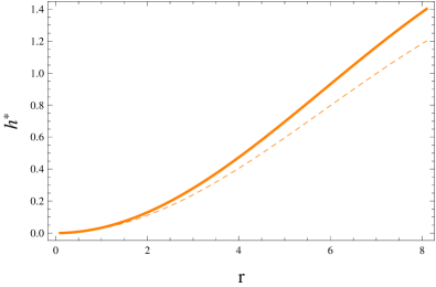
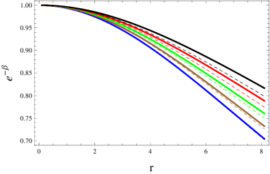
Figure 1: Plots of $h^{\ast}$ and $e^{-\beta}$ versus $r$ corresponding to $\lambda=-0.4$ (solid), $-0.5$ (dashed), $\delta=0.01$ (blue), $0.03$ (brown), $0.05$ (green), $0.07$ (red) and $0.09$ (black) for solution I.

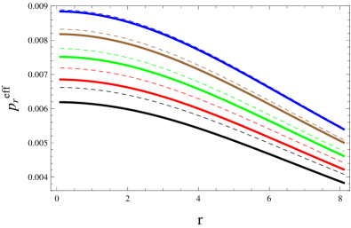
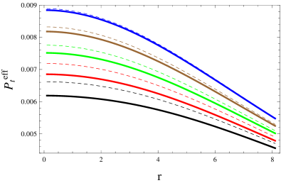
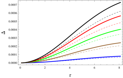
Figure 2: Plots of $\rho^{eff},P_{r}^{eff},P_{t}^{eff}$ and $\Delta$ versus $r$ corresponding to $\lambda=-0.4$ (solid), $-0.5$ (dashed), $\delta=0.01$ (blue), $0.03$ (brown), $0.05$ (green), $0.07$ (red) and $0.09$ (black) for solution I.

The interior metric functions (41) and (50) denote the minimally deformed Finch-Skea solution by virtue of Eq.(48). We can now obtain the expressions for the effective parameters together with the induced anisotropy, jointly constituting the anisotropic solution. Due to lengthy expressions, we have displayed these parameters in the appendix.

We now discuss the graphical analysis of the effective parameters $\rho^{eff}$, $P_{r}^{eff}$, $P_{t}^{eff}$ and the anisotropy $\Delta$ for solution I. The graphical analysis is carried out using the star candidate Her X-1 with mass $M_{0}=0.85M_{\bigodot}$ and radius $R=8.1km$ [53]. We use two values of the Rastall parameter, given by $\lambda=-0.4,-0.5,$ and the coupling constant as $\delta=0.01,0.03,0.05,0.07,0.09$. We mention here that these parametric values are chosen after a long trial of values for which they were found to induce the desired behavior in the graphical analysis of the obtained models. We highlight the importance of investigating the effect of the fluctuation of the Rastall and decoupling parameters. It is essential to study the impact of the Rastall parameter as it creates the sole deviation of Rastall theory from general relativity. As for the decoupling parameter $\delta$, its essence lies in the fact that it sets the stage for the gravitational decoupling process, as it is through this parameter that the anisotropic extra source is gravitationally coupled to the isotropic seed source. Figure 1 shows the deformation function $(h^{\ast})$ and deformed radial coefficient. As expected from the deformation function, it vanishes at the core. The behavior of the effective parameters (energy density, radial and tangential pressures) ought to be finite, positive and maximum at the center whilst exhibiting a monotonically decreasing behavior towards the star’s surface, as shown in Figure 2. It is observed that the density attains lower values for the Rastall parameter $\lambda=-0.4$ as compared to its other value, leading to the conclusion that an increment in the Rastall parameter makes the interior of compact star less dense. A similar observation is made with regards to the radial and tangential pressures. In addition, the radial and tangential pressures attain the same values at the core and thus induce an anisotropy that vanishes at that point and increases towards the surface. This positive anisotropy depicts an outward directed pressure by virtue of which the anti-gravitational force is produced, helping in stabilizing the compact structure. A higher anisotropy is obtained with a reduction of the Rastall parameter.

4.3 Solution II

Here we adopt a new constraint to derive a second anisotropic solution. This constraint is imposed on the density parameter and is taken to be

$$\Theta_{0}^{0}(r)=\rho(r)\,.$$ (51)

Using Eqs.(28) and (30) in the constraint above, we have

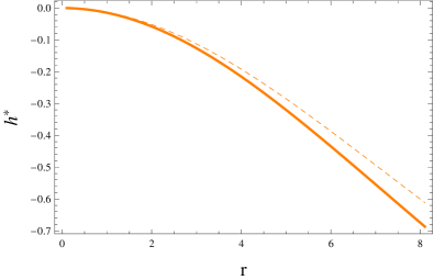
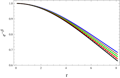
Figure 3: Plots of $h^{\ast}$ and $e^{-\beta}$ versus $r$ corresponding to $\lambda=-0.4$ (solid), $-0.5$ (dashed), $\delta=0.01$ (blue), $0.03$ (brown), $0.05$ (green), $0.07$ (red) and $0.09$ (black) for solution II.

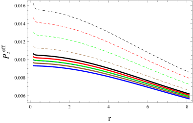
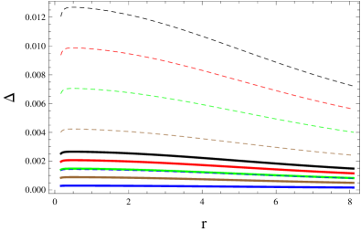
Figure 4: Plots of $\rho^{eff},P_{r}^{eff},P_{t}^{eff}$ and $\Delta$ versus $r$ corresponding to $\lambda=-0.4$ (solid), $-0.5$ (dashed), $\delta=0.01$ (blue), $0.03$ (brown), $0.05$ (green), $0.07$ (red) and $0.09$ (black) for solution II.

$$-\frac{h^{\ast^{\prime}}}{r}-\frac{h^{\ast}}{r^{2}}=\frac{1}{r^{2}}-\frac{\sigma^{\prime}}{r}-\frac{\sigma}{r^{2}}-\lambda\bigg{[}\frac{4}{r^{2}}-\frac{\sigma^{\prime}}{r}-\sigma\bigg{(}\frac{3\eta^{\prime}}{r}+\frac{4}{r^{2}}\bigg{)}\bigg{]}\,.$$ (52)

Due to the unavailability of an exact solution of the differential equation (52), we proceed with a numerical approximation. The graphical description for solution II follows exactly as in the case of solution I. The deformation function and the deformed radial coefficient are obtained and shown in Figure 3. The effective parameters and anisotropy are also obtained and plotted in Figure 4. As the case of the solution I, they exhibit a behavior consistent with compact stars (i.e., positive, finite, maximum at the core and monotonically decreasing towards the boundary). However, in contrast to solution I, it is observed here that an increment in the Rastall parameter makes the interior of compact stars more dense. The effect of the increment in the Rastall parameter is seen to coincide with a reduction in the radial and tangential pressures. Due to the inequality of the radial and tangential pressures at the core, the corresponding anisotropy is non-vanishing at the core and possesses a positive profile everywhere.

4.4 Analysis of Physical Viability and Stability

Here, we shall investigate various physical features of both solutions, ranging from physical viability to stability. The energy conditions are physical restrictions imposed on the stress-energy tensor and (if satisfied) portray the existence of ordinary matter in the interior of stellar distribution. These conditions can be classified as dominant, strong, weak and null energy conditions as follows.

• Dominant Energy Conditions
  $\rho^{eff}-P_{r}^{eff}\geq 0,\quad\rho^{eff}-P_{t}^{eff}\geq 0.$

• Strong Energy Conditions
  $\rho^{eff}+P_{r}^{eff}\geq 0,\quad\rho^{eff}+P_{t}^{eff}\geq 0,\quad\rho^{eff}+P_{r}^{eff}+2P_{t}^{eff}\geq 0.$

• Weak Energy Conditions
  $\rho^{eff}\geq 0,\quad\rho^{eff}+P_{r}^{eff}\geq 0,\quad\rho^{eff}+P_{t}^{eff}\geq 0.$

• Null Energy Conditions
  $\rho^{eff}+P_{r}^{eff}\geq 0,\quad\rho^{eff}+P_{t}^{eff}\geq 0.$

As seen in Figures 5 and 6, all the energy bounds are met by our obtained solutions thereby implying physical viability. We also investigate an interesting physical feature of celestial objects, dubbed the EoS parameter. With respect to the radial and tangential EoS denoted by $\omega_{r}=\frac{P_{r}^{eff}}{\rho^{eff}}$ and $\omega_{t}=\frac{P_{t}^{eff}}{\rho^{eff}}$, respectively, an effective stellar configuration is implied if $0\leq\omega_{r}\leq 1$ and $0\leq\omega_{t}\leq 1$ [54]. This condition is also satisfied by both solutions as shown in Figure 7.

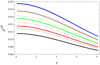
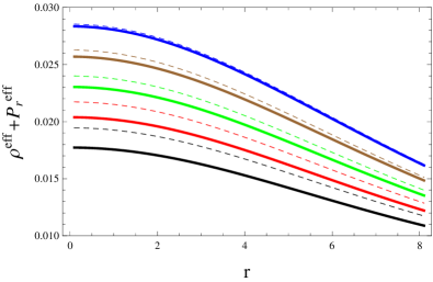
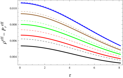
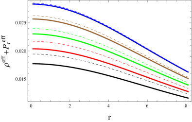
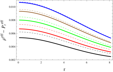
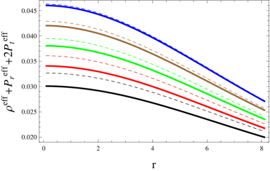
Figure 5: Plots of energy conditions versus $r$ corresponding to $\lambda=-0.4$ (solid), $-0.5$ (dashed), $\delta=0.01$ (blue), $0.03$ (brown), $0.05$ (green), $0.07$ (red) and $0.09$ (black) for solution I.

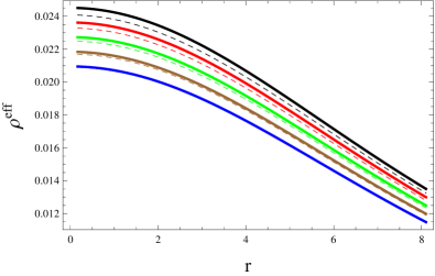
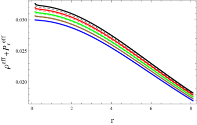
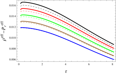
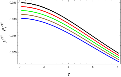
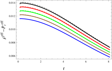
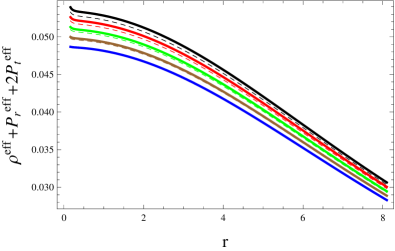
Figure 6: Plots of energy conditions versus $r$ corresponding to $\lambda=-0.4$ (solid), $-0.5$ (dashed), $\delta=0.01$ (blue), $0.03$ (brown), $0.05$ (green), $0.07$ (red) and $0.09$ (black) for solution II.

Additionally, we examine the compactness $u(r)=\frac{m(r)}{r}$ and surface redshift $Z_{s}=\frac{1}{\sqrt{1-2u(r)}}-1$. The compactness of a celestial body describes how densely its mass is packed within a specific volume or radius. This measure is dimensionless and helps to determine the intensity of the gravitational field at the object’s surface. On the other hand, surface redshift refers to the shift in the wavelength of light or electromagnetic radiation emitted from the surface of a dense object when viewed from a distance. The powerful gravitational pull near the object’s surface causes the light to lose energy, resulting in a longer wavelength, or redshift. With these parameters, the limits $u(r)<\frac{4}{9}$ [55] and $Z_{s}\leq 5.2$ [56] guaranty an effective matter configuration. It can be observed that the surface redshift is dependent on the compactness function which, in turn, depends on the mass function. The mass of the sphere can be determined by the equation

$$m(r)=4\pi\int_{0}^{r}\rho^{eff}r^{2}dr.$$ (53)

Both solutions satisfy the stated compactness and surface redshift limits as shown in their plots displayed in Figure 8.

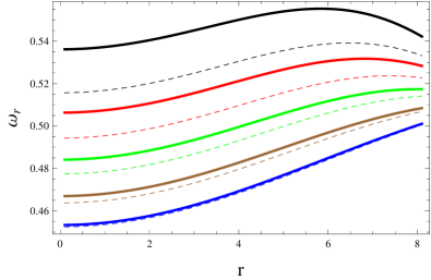
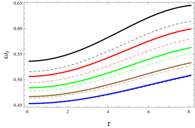
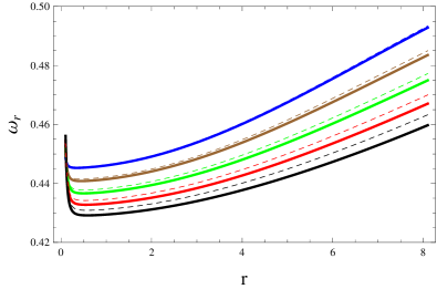
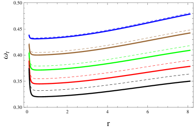
Figure 7: Plots of radial and tangential EoS parameters versus $r$ corresponding to $\lambda=-0.4$ (solid), $-0.5$ (dashed), $\delta=0.01$ (blue), $0.03$ (brown), $0.05$ (green), $0.07$ (red) and $0.09$ (black) for solutions I (top row) and II (bottom row).

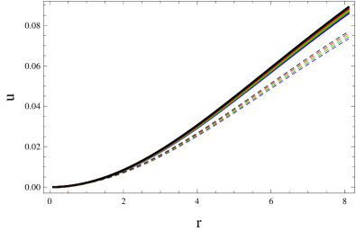
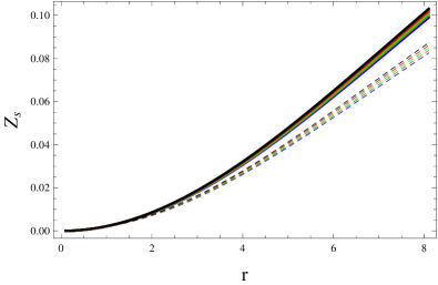
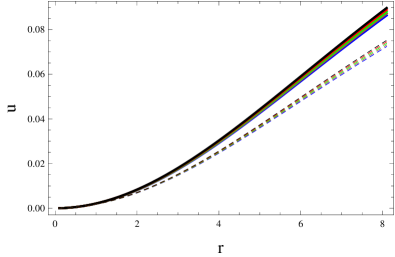
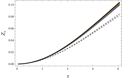
Figure 8: Plots of compactness and surface redshift versus $r$ corresponding to $\lambda=-0.4$ (solid), $-0.5$ (dashed), $\delta=0.01$ (blue), $0.03$ (brown), $0.05$ (green), $0.07$ (red) and $0.09$ (black) for solutions I (top row) and II (bottom row).

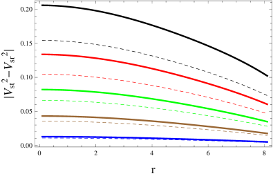
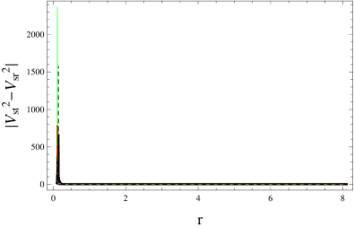
Figure 9: Plots of $|V_{st}^{2}-V_{sr}^{2}|$ versus $r$ corresponding to $\lambda=-0.4$ (solid), $-0.5$ (dashed), $\delta=0.01$ (blue), $0.03$ (brown), $0.05$ (green), $0.07$ (red) and $0.09$ (black) for solutions I (left) and II (right).

We now shift our focus to the stability analysis of the obtained solutions. We first use the Herrera cracking technique [20] in which stability demands that $0\leq|V_{st}^{2}-V_{sr}^{2}|\leq 1$, where $V_{st}^{2}=\frac{dP_{t}^{eff}}{d\rho^{eff}}$ and $V_{sr}^{2}=\frac{dP_{r}^{eff}}{d\rho^{eff}}$ denote the tangential and radial sound speeds, respectively. Through this test, we show that solution I is stable while solution II is unstable (Figure 9). The stability of both solutions is further tested using the causality condition wherein stability necessitates that the speed of sound components must be contained in the range $\left[0,~{}1\right]$, i.e., $0\leq V_{sr}^{2}\leq 1$ and $0\leq V_{st}^{2}\leq 1\,.$ The results of this test which are shown in Figure 10, corroborates the outcome of the Herrera cracking test. The plot of the Herrera cracking condition for solution II (in the right panel of Figure 9) as well as the plots of the causality conditions for solution II (in the bottom panel of Figure 10) display unbounded behavior at the core. This behavior at the core can be attributed to the instability of the said model. We highlight that the discontinuity portrayed at the core, in some of the matter variables (for solution II) plotted in Figures 4 and 6 are in line with the obtained results for the stability of this model. This behavior is the characteristic of an unstable model as deduced through the aforementioned stability analysis.

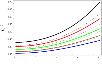
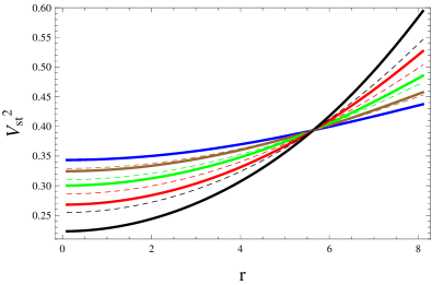
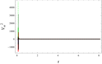
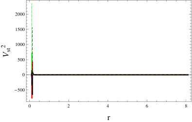
Figure 10: Plots of radial and tangential sound speeds versus $r$ corresponding to $\lambda=-0.4$ (solid), $-0.5$ (dashed), $\delta=0.01$ (blue), $0.03$ (brown), $0.05$ (green), $0.07$ (red) and $0.09$ (black) for solutions I (top row) and II (bottom row).

5 Conclusions

Numerous researchers are involved in the search for interior solutions defining self-gravitating systems. To this end, astrophysicists have made several efforts to build stable and physically viable solutions for compact objects. Recently, the MGD technique has been widely applied to obtain precise solutions for the internal constitution of stellar objects. In this paper, we have used this approach to obtain anisotropic spherical solutions by extending a known isotropic interior solution, namely, the Finch-Skea ansatz. The static and spherically symmetric Rastall field equations (15)-(17) have been decoupled into two sets, the first set corresponding to the Rastall field equations (24)-(26) for isotropic matter distribution $\bar{T}_{\tau\upsilon}$ while the second set (30)-(32) characterizes the anisotropic source $\Theta_{\tau\upsilon}\,.$ The junction conditions that govern the smooth matching at the stellar surface have also been studied, taking the exterior geometry to be the Schwarzschild spacetime.

Since the Rastall theory of gravity contains an extra term that deviates from general relativity, we have investigated the effects of this term in this work. To extend the Finch-Skea solution to an anisotropic domain, we have followed the same procedure given in [16]. Using the mimic constraint approach, we impose suitable conditions that relate the thermodynamic seed variables with the corresponding components of the $\Theta$-sector so that the decoupling function $h^{\ast}(r)$ can be determined. We have thus used two constraints: a pressure-like constraint in which the $1-1$ component of the $\Theta$-sector mimics the seed pressure $P(r)$, and a density-like constraint in which the $0-0$ component mimics seed energy density $\rho(r)$. In the case of solution I, a simple algebraic equation has been obtained from which an explicit expression for the decoupling function is easily derived. However, for solution II, a first order differential equation has appeared from which a numerical solution of the decoupling function is obtained due to mathematical complications introduced by the Rastall contribution $G_{\lambda}(r)$.

For the Rastall parameter $\lambda=-0.4,-0.5~{}$ with the decoupling constant $~{}\delta=0.01,0.03,0.05,0.07,0.09,$ the physical behavior of the effective parameters for both solutions have been found to be in agreement with the requirements for compact stars. The generated anisotropy in both cases has been found to be positive, implying an outward directed pressure that produces the anti-gravitational force necessary to keep the compact object in an equilibrium state. We have found that increasing the value of $\lambda$ provides a less dense interior of compact stars in the case of solution I and a more dense interior corresponding to solution II. We have also found that increasing the value of the decoupling parameter $\delta$ enhances a less dense interior of compact stars in the case of solution I and a more dense interior corresponding to solution II. In addition, the physical viability of both solutions has been endorsed through analysis of the energy conditions. Stability analysis has also been done through the Herrera cracking and causality condition through which we have established that solution I is stable while solution II is unstable. We would like to point out that such tests for physical viability and stability have not been executed in the case of general relativity [16]. Finally, all our results can be reduced to general relativity for $\lambda=0$.

Appendix: Effective parameters $\rho^{eff},P_{r}^{eff},P_{t}^{eff}$ and Anisotropy $\Delta$

$$\rho^{eff} =\frac{C\sqrt{Cr^{2}}}{\left(Cr^{2}+1\right)^{3}\left(2A+Br\sqrt{Cr^{2}}\right)}$$

$$\times\bigg{[}\frac{\left(Cr^{2}+1\right)\left(Cr^{2}+3\right)\left(4A\left(A+Br\sqrt{Cr^{2}}\right)+B^{2}Cr^{4}\right)}{2A\sqrt{Cr^{2}}+BCr^{3}}$$

$$+\frac{C\sqrt{Cr^{2}}}{\left(BCr^{3}\left(4\ln\left(A+\frac{1}{2}Br\sqrt{Cr^{2}}\right)+1\right)+2A\sqrt{Cr^{2}}\right)^{2}}$$

$$\times\bigg{(}8A^{3}\sqrt{Cr^{2}}\left(Cr^{2}\left(C(4\lambda-1)r^{2}+14\lambda-4\right)+18\lambda-3\right)$$

$$+4Br\ln\left(A+\frac{1}{2}Br\sqrt{Cr^{2}}\right)\bigg{(}4A^{2}\bigg{(}Cr^{2}\bigg{(}Cr^{2}\left(C(1-4\lambda)r^{2}-9\lambda+1\right)$$

$$-6\lambda+3\bigg{)}-9\lambda+3\bigg{)}+4Br(3\lambda-1)\left(C^{2}r^{4}-1\right)\left(2A\sqrt{Cr^{2}}+BCr^{3}\right)$$

$$\times\ln\left(A+\frac{1}{2}Br\sqrt{Cr^{2}}\right)+8ABr\sqrt{Cr^{2}}\bigg{(}Cr^{2}\left(C(2\lambda-1)r^{2}+3\lambda\right)$$

$$-3\lambda+1\bigg{)}+B^{2}Cr^{4}\bigg{(}Cr^{2}\left(Cr^{2}\left(C(4\lambda-1)r^{2}+17\lambda-5\right)+18\lambda-3\right)$$

$$-3\lambda+1\bigg{)}\bigg{)}+12A^{2}BCr^{3}\left(Cr^{2}\left(C(4\lambda-1)r^{2}+14\lambda-4\right)+18\lambda-3\right)$$

$$+2AB^{2}r^{2}\sqrt{Cr^{2}}\bigg{(}Cr^{2}\left(Cr^{2}\left(5C(1-4\lambda)r^{2}-62\lambda+12\right)-42\lambda+15\right)$$

$$-24\lambda+8\bigg{)}+B^{3}Cr^{5}\bigg{(}Cr^{2}\bigg{(}Cr^{2}\left(7C(1-4\lambda)r^{2}-90\lambda+20\right)$$

$$-78\lambda+21\bigg{)}-24\lambda+8\bigg{)}\bigg{)}\bigg{]},$$

$$P_{r}^{eff} =\frac{4BCr\left(Cr^{2}+1\right)(\delta(3\lambda-1)+1)\ln\left(A+\frac{1}{2}Br\sqrt{Cr^{2}}\right)}{\sqrt{Cr^{2}}\left(Cr^{2}+1\right)^{2}\left(2A+Br\sqrt{Cr^{2}}\right)}$$

$$-\frac{C\left(2A\sqrt{Cr^{2}}+Bcr^{3}\right)\bigg{(}Cr^{2}(4\delta\lambda-\delta+1)+6\delta\lambda-\delta+1\bigg{)}}{\sqrt{Cr^{2}}\left(Cr^{2}+1\right)^{2}\left(2A+Br\sqrt{Cr^{2}}\right)},$$

$$P_{t}^{eff} =\frac{C}{\left(Cr^{2}+1\right)^{3}\left(2A+Br\sqrt{Cr^{2}}\right)^{2}}$$

$$\times\bigg{[}\bigg{(}\frac{(1+Cr^{2})^{2}4B\left(2A\sqrt{Cr^{2}}+BCr^{3}\right)\ln\left(A+\frac{1}{2}Br\sqrt{Cr^{2}}\right)}{Cr}$$

$$-\frac{(1+Cr^{2})^{2}Cr\left(4A\left(A+Br\sqrt{Cr^{2}}\right)+B^{2}Cr^{4}\right)}{Cr}\bigg{)}$$

$$+\frac{\delta}{\left(BCr^{3}\left(4\ln\left(A+\frac{1}{2}Br\sqrt{Cr^{2}}\right)+1\right)+2A\sqrt{Cr^{2}}\right)^{2}}$$

$$\times\bigg{(}\left(BCr^{3}\left(2\ln\left(A+\frac{1}{2}Br\sqrt{Cr^{2}}\right)+1\right)+2A\sqrt{Cr^{2}}\right)$$

$$\times\bigg{(}8A^{3}\sqrt{Cr^{2}}\left(C(1-2\lambda)r^{2}-6\lambda+1\right)+4Br\ln\left(A+\frac{1}{2}Br\sqrt{Cr^{2}}\right)$$

$$\times\bigg{(}4A^{2}\left(Cr^{2}\left(Cr^{2}\left(C(4\lambda-1)r^{2}+8\lambda-1\right)+3\lambda-1\right)+3\lambda-1\right)$$

$$+2ABr\sqrt{Cr^{2}}\left(Cr^{2}\left(Cr^{2}\left(C(4\lambda-1)r^{2}+3\lambda+1\right)-6\lambda+1\right)+3\lambda-1\right)$$

$$-4BC(3\lambda-1)r^{3}\left(Cr^{2}+1\right)\left(2A\sqrt{Cr^{2}}+BCr^{3}\right)\ln\left(A+\frac{1}{2}Br\sqrt{Cr^{2}}\right)$$

$$+B^{2}C^{2}r^{6}\left(C(2-5\lambda)r^{2}-9\lambda+2\right)\bigg{)}+12A^{2}BCr^{3}\left(C(1-2\lambda)r^{2}-6\lambda+1\right)$$

$$+2AB^{2}r^{2}\sqrt{Cr^{2}}\bigg{(}Cr^{2}\left(Cr^{2}\left(4C(4\lambda-1)r^{2}+46\lambda-9\right)+30\lambda-9\right)$$

$$+12\lambda-4\bigg{)}+B^{3}Cr^{5}\bigg{(}Cr^{2}\left(Cr^{2}\left(4C(4\lambda-1)r^{2}+50\lambda-11\right)+42\lambda-11\right)$$

$$+12\lambda-4\bigg{)}\bigg{)}-4Br\sqrt{Cr^{2}}\left(Cr^{2}+1\right)\bigg{(}Br\sqrt{Cr^{2}}2\ln\left(A+\frac{1}{2}Br\sqrt{Cr^{2}}\right)$$

$$+2A\ln\left(A+\frac{1}{2}Br\sqrt{Cr^{2}}\right)+Br\sqrt{Cr^{2}}\bigg{)}\bigg{(}BCr^{3}\bigg{(}4\ln\left(A+\frac{1}{2}Br\sqrt{Cr^{2}}\right)$$

$$+1\bigg{)}+2A\sqrt{Cr^{2}}\bigg{)}\bigg{(}\left(C(4\lambda-1)r^{2}+6\lambda-1\right)\left(2A\sqrt{Cr^{2}}+BCr^{3}\right)$$

$$-4B(3\lambda-1)r\left(Cr^{2}+1\right)\ln\left(A+\frac{1}{2}Br\sqrt{Cr^{2}}\right)\bigg{)}\bigg{)}\bigg{]},$$

$$\Delta =\frac{\delta\,C}{\left(Cr^{2}+1\right)^{3}\left(2A+Br\sqrt{Cr^{2}}\right)^{2}}\bigg{[}\bigg{(}\frac{\left(Cr^{2}+1\right)\left(2A+Br\sqrt{Cr^{2}}\right)}{\sqrt{Cr^{2}}}$$

$$\times\bigg{(}\left(C(4\lambda-1)r^{2}+6\lambda-1\right)\left(2A\sqrt{Cr^{2}}+BCr^{3}\right)$$

$$-4B(3\lambda-1)r\left(Cr^{2}+1\right)\ln\left(A+\frac{1}{2}Br\sqrt{Cr^{2}}\right)\bigg{)}\bigg{)}$$

$$-\frac{1}{BCr^{3}\left(4\ln\left(A+\frac{1}{2}Br\sqrt{Cr^{2}}\right)+1\right)+2A\sqrt{Cr^{2}}}$$

$$\times 4Br\sqrt{Cr^{2}}\left(Cr^{2}+1\right)\bigg{(}Br\sqrt{Cr^{2}}\ln^{2}\left(A+\frac{1}{2}Br\sqrt{Cr^{2}}\right)$$

$$+2A\ln\left(A+\frac{1}{2}Br\sqrt{Cr^{2}}\right)+Br\sqrt{Cr^{2}}\bigg{)}\bigg{(}\left(C(4\lambda-1)r^{2}+6\lambda-1\right)$$

$$\times\left(2A\sqrt{Cr^{2}}+BCr^{3}\right)-4B(3\lambda-1)r\left(Cr^{2}+1\right)\ln\left(A+\frac{1}{2}Br\sqrt{Cr^{2}}\right)\bigg{)}$$

$$+\frac{1}{\left(BCr^{3}\left(4\ln\left(A+\frac{1}{2}Br\sqrt{Cr^{2}}\right)+1\right)+2A\sqrt{Cr^{2}}\right)^{2}}\bigg{(}BCr^{3}\bigg{(}2\ln\bigg{(}A$$

$$+\frac{1}{2}Br\sqrt{Cr^{2}}\bigg{)}+1\bigg{)}+2A\sqrt{Cr^{2}}\bigg{)}\bigg{(}8A^{3}\sqrt{Cr^{2}}\left(C(1-2\lambda)r^{2}-6\lambda+1\right)$$

$$+4Br\ln\left(A+\frac{1}{2}Br\sqrt{Cr^{2}}\right)\bigg{(}4A^{2}\bigg{(}Cr^{2}\left(Cr^{2}\left(C(4\lambda-1)r^{2}+8\lambda-1\right)+3\lambda-1\right)$$

$$+3\lambda-1\bigg{)}+2ABr\sqrt{Cr^{2}}\left(cr^{2}\left(Cr^{2}\left(C(4\lambda-1)r^{2}+3\lambda+1\right)-6\lambda+1\right)+3\lambda-1\right)$$

$$-4BC(3\lambda-1)r^{3}\left(Cr^{2}+1\right)\left(2A\sqrt{Cr^{2}}+BCr^{3}\right)\ln\left(A+\frac{1}{2}Br\sqrt{Cr^{2}}\right)+B^{2}C^{2}r^{6}$$

$$\times\left(C(2-5\lambda)r^{2}-9\lambda+2\right)\bigg{)}+12A^{2}BCr^{3}\left(C(1-2\lambda)r^{2}-6\lambda+1\right)$$

$$+2AB^{2}r^{2}\sqrt{Cr^{2}}\bigg{(}Cr^{2}\left(Cr^{2}\left(4C(4\lambda-1)r^{2}+46\lambda-9\right)+30\lambda-9\right)$$

$$+12\lambda-4\bigg{)}+B^{3}Cr^{5}\bigg{(}Cr^{2}\bigg{(}Cr^{2}\bigg{(}4C(4\lambda-1)r^{2}+50\lambda-11\bigg{)}$$

$$+42\lambda-11\bigg{)}+12\lambda-4\bigg{)}\bigg{)}\bigg{]}.$$

Data Availability Statement: No data was used for the research described in this paper.

References

- [1] Rastall, P.: Phys. Rev. D 6(1972)3357.
- [2] Heydarzade, Y. and Darabi, F.: Phys. Lett. B 771(2017)365.
- [3] Licata, I., Moradpour, H. and Corda, C.: Int. J. Geom. Methods Mod. Phys. 14(2017)1730003.
- [4] Xu, Z., Hou, X., Gong, X. and Wang, J.: Eur. Phys. J. C 78(2018)01; Graca, J.M. and Lobo, I.P.: Eur. Phys. J. C 78(2018)101; Kumar, R. and Ghosh, S.G.: Eur. Phys. J. C. 78(2018)750; Bamba, K., Jawad, A., Rafique, S. and Moradpour, H.: Eur. Phys. J. C 78(2018)986.
- [5] Fabris, J.C. et al.: Int. J. Mod. Phys. D 27(2018)1841006; Spallucci, E. and Smailagic, A.: Int. J. Mod. Phys. D 27(2018)1850003; Lobo, I.P., Moradpour, H., Morais Graça, J.P. and Salako, I.G.: Int. J. Mod. Phys. D 27(2018)1850069.
- [6] Darabi, F., Atazadeh, K. and Heydarzade, Y.: Eur. Phys. J. Plus 133(2018)249.
- [7] Haghani, Z., Harko, T. and Shahidi, S.: Phys. Dark Universe 21(2018)27.
- [8] Visser, M.: Phys. Lett. B 782(2018)83.
- [9] Ovalle, J.: Mod. Phys. Lett. A 23(2008)3247.
- [10] Randall, L. and Sundrum, R.: Phys. Rev. Lett. 83(1999)3370; ibid. 4690
- [11] Casadio, R., Ovalle, J. and Da Rocha, R.: Class. Quantum Grav. 32(2015)215020.
- [12] Ovalle, J.: Int. J. Mod. Phys.: Conf. Ser. 41(2016)1660132.
- [13] Ovalle, J. and Linares, F.: Phys. Rev. D 88(2013)104026.
- [14] Casadio, R., Ovalle, J. and Da Rocha, R.: Class. Quantum Grav. 32(2015)215020.
- [15] Ovalle, J.: Phys. Rev. D 95(2017)104019.
- [16] Ovalle, J., Casadio, R., Da Rocha, R. and Sotomayor, A.: Eur. Phys. J. C 78(2018)122.
- [17] Mak, M.K., Dobson, Jr., P.N. and Harkó, T.: Int. J. Mod. Phys. D 11(2002)207; Mak, M.K. and Harkó, T.: Proc. Roy. Soc. Lond. A 459(2003)393
- [18] Gleiser, M. and Dev, K.: Int. J. Mod. Phys. D 13(2004)1389.
- [19] Sharma, R. and Maharaj, S.D.: Mon. Not. R Astron. Soc. 375(2007)1265.
- [20] Herrera, L.: Phys. Lett. A 165(1992)206.
- [21] Abreu, H., Hernández, H. and Núñez, L.A.: J. Phys.: Conf. Ser. 66(2006)012038.
- [22] Maurya, S.K. and Govender, M.: Eur. Phys. J. C 77(2017)420.
- [23] Colpi, M., Shapiro, S.L. and Wasserman, I.: Phys. Rev. Lett. 57(1986)2485.
- [24] Schunck, F.E. and Mielke, E.W.: Class. Quantum Grav. 20(2003)R301.
- [25] Zloshchastiev, K.G.: Phys. Rev. Lett. 94(2005)121101.
- [26] Dzhunushaliev, V., Folomeev, V., Myrzakulov, R. and Singleton, D.: J. High Energy Phys. 0807(2008)094.
- [27] Lü, H., Perkins, A., Pope, C. N. and Stelle, K. S.: Phys. Rev. Lett. 114(2015)171601.
- [28] Chakraborty, S. and SenGupta, S.: Eur. Phys. J. C 76(2016)552.
- [29] Kokkotas, K.D., Konoplya, R.A. and Zhidenko, A.: Phys. Rev. D 96(2017)064007.
- [30] De Felice, A. and Tsujikawa, S.: Living Rev. Rel. 13(2010)3.
- [31] Sotiriou, T.P. and Faraoni, V.: Rev. Mod. Phys. 82(2010)451.
- [32] Capozziello, S. and De Laurentis, M.: Phys. Rep. 509(2011)167.
- [33] Capozziello, S., Cardone, V. F. and Troisi, A.: Phys. Rev. D 71(2005)043503.
- [34] Jaime, L.G., Patino, L. and Salgado, M.: Phys. Rev. D 83(2011)024039.
- [35] Caate, P., Jaime, L.G. and Salgado, M.: Class. Quantum Grav. 33(2016)155005.
- [36] Alvarez-Gaume, L., Kehagias, A., Kounnas, C., Lust, D. and Riotto, A.: Fortschr. Phys. 64(2016)176.
- [37] Vernieri, D. and Carloni, S.: Eur. Phy. Lett. 121(2018)30002.
- [38] Eling, C. and Jacobson, T.: Class. Quantum Grav. 23(2006)5625.
- [39] Stuchlík, Z., Hledik, S. and Novotnỳ, J.: Phys. Rev. D 94(2016)103513.
- [40] Novotnỳ, J., Hladik, J. and Stuchlík, Z.: Phys. Rev. D 95(2017)043009.
- [41] Stuchlík, Z., Schee, J., Toshmatov, B., Hladik, J. and Novotnỳ, J.: J. Cosmol. Astropart. Phys. 06(2017)056.
- [42] Stephani, H., Kramer, D., MacCallum, M., Hoenselaers, C. and Herlt, E.: Exact Solutions of Einstein’s Field Equations (Cambridge University Press, 2003).
- [43] Finch, M.R. and Skea, J.E.F.: Class. Quantum Grav. 6(1989)467.
- [44] Sharif, M. and Sadiq, S.: Eur. Phys. J. C 78(2018)410.
- [45] Sharif, M. and Majid, A.: Chin. J. Phys. 68(2020)406; Phys. Dark Universe 30(2020)100610.
- [46] Sharif, M. and Saba, S.: Chin. J. Phys. 63(2020)348; Int. J. Mod. Phys. D 29(2020)2050041.
- [47] Sharif, M. and Naseer, T.: Chin. J. Phys. 73(2021)179; Universe 8(2022)62.
- [48] Sharif, M. and Hassan, K.: Eur. Phys. J. Plus 137(2022)997; Universe 9(2023)165.
- [49] Maurya, S.K. and Tello-Ortiz, F.: Phys. Dark Universe 29(2020)100577.
- [50] Sharif, M. and Sallah, M.: New Astron. 109(2024)102198.
- [51] Ovalle, J. et al.: Eur. Phys. J. C 78(2018)960.
- [52] Sharif, M. and Majid, A.: Phys. Scr. 96(2021)035002.
- [53] Abubekerov, M.K., Antokhina, E.A., Cherepashchuk, A.M. and Shimanskii, V.V.: Astron. Rep. 52(2008)379
- [54] Shamir, M.F. and Zia, S.: Eur. Phys. J. C 77(2017)448.
- [55] Buchdahl, H.A.: Phys. Rev. 116(1959)1027.
- [56] Ivanov, B.V.: Phys. Rev. D 65(2002)104011.