Free cumulants and freeness for unitarily invariant random tensors
Abstract
We address the question of the asymptotic description of random tensors that are local unitary invariant, that is, invariant by conjugation by tensor products of (independent) unitary matrices. We consider both the case of an invariant random tensor with inputs and outputs, called mixed, and the case where there is a factorization between the inputs and outputs, called pure, and which includes the random tensor models that have been extensively studied in the physics literature (we provide a short review of these results).
The finite size and asymptotic moments are defined in terms of the correlations of certain invariant polynomials called trace-invariants, encoded by -uplets of permutations, up to relabelling equivalence. Using the unitary invariance, we define a notion of finite free cumulants associated to the expectations of these trace-invariants, through invertible finite size moment-cumulants formulas.
In order to characterize the asymptotic distributions at first order, two important classes of random tensors are considered: pure random tensors that scale like a pure complex Gaussian, and mixed random tensors that scale like a Wishart tensor. In both cases, we derive a notion of free cumulants associated to the first order trace-invariants, through closed moment-cumulant formulas, which involve independent summations over non-crossing permutations. While the formulas involve the same combinatorics, the asymptotic distributions differ by the class of invariants that define the distribution at first order. Both in the pure and in the mixed case, the first order free-cumulants of a sum of two independent random tensors are shown to be additive. A preliminary discussion of the higher orders is provided. Finally, tensor freeness is then defined (at first order) as the vanishing of mixed free cumulants associated to first order trace-invariants.
1 Introduction
In this paper, tensors are arrays of complex numbers of the form , where all indices take value in for some . Tensors for which the components factor as are called pure, in which case , and tensor for which they do not are called mixed. We study in this paper random tensors whose probability measure is local-unitary invariant, or LU-invariant, that is invariant upon conjugation by a tensor product of unitary matrices: and have the same distribution for any , where is the set of unitary matrices.
Examples of such probability distributions include the pure complex Gaussian as well as perturbed Gaussian models, for which the probability density function of the Gaussian is altered by the addition of an invariant potential, see e.g. [21, 25, 26, 28, 29, 30, 32, 33]. Regarding random tensors, see also [34, 45, 35, 36, 37, 38, 39, 40, 41, 42, 43, 44]. Such models were initially studied because they provide generating functions for random triangulations relevant for the study random geometry and quantum gravity. Example of mixed distributions include Wishart tensors formed by partially tracing pure tensors, or a GUE random matrix with subdivided index sets.
Another important motivation for studying LU-invariant distribution comes from quantum entanglement. Consider a -partite quantum system. Its state space is a Hilbert space with a tensor product structure , and we assume that for all , for some . Seen as density matrices, pure quantum state are projectors , and fixing an orthonormal basis in each factor , decomposes as:
Component-wise, a pure density matrix corresponds to a pure tensor , with a normalization condition. A mixed density matrix is a positive semi definite operator:
with a normalization condition. Thus, mixed density matrices correspond to normalized mixed tensors. This explains the terminology.
Local unitary invariance plays an important role in quantum information: such transformations - which correspond to local changes of orthonormal basis in each - don’t affect the entanglement between the subsystems. In fact, local unitary invariance is sometimes introduced as a definition of equivalent entanglement [66, 67, 68, 69], although in this context a more operational definition of equivalent entanglement is often preferred. However, local unitary invariance always plays an important role in multipartite entanglement: entanglement measures are LU-invariant, two-ways LOCC is equivalent to LU-equivalence, and so on. In order to study the entanglement properties of classes of quantum states that are equivalently entangled, one introduces distributions on the tensor coefficients of the states and, since LU-transformations don’t affect entanglement, it is necessary to require that these distributions are LU-invariant.
In this paper, we address the question of how to characterize a LU-invariant random tensor distribution starting from its moments. Results in invariant theory justify our choice to characterize such distributions by the expectations of invariant homogeneous polynomials [58, 59, 60, 61, 64]. Our purpose is to ultimately study the distributions asymptotically, when the size of the index set (or the dimension) goes to infinity, while the number of indices (or subsystems) stays constant. Generalizing the approach of [7], we discuss which quantities play the role of asymptotic moments, a choice which generally differs for mixed and pure random tensors. A notion of order is introduced, related to how the finite quantities must be rescaled in order to obtain the asymptotic moments. First order asymptotic moments are those which require the strongest rescaling.
For non-commutative random variables, freeness, or free independence, is a notion of independence which is weaker than the usual independence [4, 1, 2, 3, 7, 13]. Usual independence can be formulated as the vanishing of classical cumulants. For random matrices, asymptotic freeness in the limit can be characterized by the vanishing of free cumulants (or first order free cumulants), a sequence of numbers which represent the same information as the sequence of the first order asymptotic moments. Such free cumulants are defined in terms of the first order asymptotic moments, and by Möebius inversion one can write the asymptotic moments in terms of the free cumulants.
Independent unitarily invariant random matrices are known to be asymptotically free, which implies that their free cumulants are additive. This gives access to the spectrum of the sum of two independent unitarily invariant random matrices whose spectrum is known (random Horn problem). Freeness plays a role in the study of random quantum states, see [10, 50, 47, random-state3, 48, 49, 51, 52, 53].
The pure complex Gaussian tensor ensemble is obtain by requesting that the coefficients of are independent and identically distributed complex Gaussian variables. Appropriately normalized, the vector can be written as where is a fixed pure state and is a Haar distributed random unitary matrix: the pure complex Gaussian tensor corresponds in this interpretation to taking a uniform distribution on pure quantum states. We call Wishart tensor the mixed tensor obtained by summing one of the indices of with the corresponding index of of the same position (color) . This corresponds to partially tracing the associated density matrix over one of the subsystems , obtaining the density matrix induced on the remaining subsystems.
The pure random tensors distributions whose asymptotic behavior we study here are assumed to scale at large like the pure complex Gaussian, in the sense that their asymptotic moments are obtained with the same rescaling at large . However, no other assumption is made on the asymptotic moments. The mixed tensors considered are those which scale like the Wishart tensor.
With these assumptions, using Weingarten calculus [8, 9, 12], we derive a notion of finite free cumulants by studying the expansion of the generating function of the classical cumulants (related to the tensor HCIZ integral, see [5, 6]) on the trace-invariants which play the role of moments for LU-invariant random tensors. Taking the asymptotic of these relations, we obtain combinations of first order asymptotic moments which define first order free cumulants for random tensors that satisfy our scaling assumptions, and which by construction are additive for independent random tensors. These formulas involve the same combinatorial restriction in the pure and the mixed case considered, but the asymptotic distributions differ by the classes of invariants that arise at first order. These relations can therefore be inverted in the lattice product of non-crossing partitions: knowing the first order free cumulants is equivalent to knowing the asymptotic distribution at first order.
This paper is just a first step in a vast program of study of freeness for random tensors. Further work is needed to pursue the generalization of free probability to random tensors, as well as its applications to quantum information theory, and so on.
Acknowledgments
R. G. is and L. L. has been supported by the European Research Council (ERC) under the European Union’s Horizon 2020 research and innovation program (grant agreement No 818066) and by the Deutsche Forschungs-gemeinschaft (DFG) under Germany’s Excellence Strategy EXC– 2181/1 – 390900948 (the Heidelberg STRUCTURES Cluster of Excellence). B. C. is supported by JSPS Grant-in-Aid Scientific Research (B) no. 21H00987, and Challenging Research (Exploratory) no. 20K20882 and 23K17299. L. L. receives support from CNRS grants FEI 2024 - AAP TREMPLIN-INP.
2 Notations and prerequisites
Partitions and permutations.
We will denote by be the group of permutations of elements, and the set of -uplets of permutations , . The cyclic permutation will be denoted by , and denotes the identity permutation. For , denotes the number of disjoint cycles of and the minimal number of transpositions required to obtain and .
We denote by the set of all partitions of elements. The notation is used for the number of blocks of , denotes the blocks, and the cardinal of . The refinement partial order is denoted by , that is if all the blocks of are subsets of blocks of . Furthermore, denotes the joining of partitions: is the finest partition which is coarser than both and . and respectively denote the one-block and the blocks partitions of . The partition induced by the cycles of the permutation is denoted by , hence . If is such that and if , refers to the permutation induced by on . The number of partitions of elements with parts of size is .
In particular we will encounter bipartite partitions of bipartite sets. A bipartite partition of the bipartite set is a partition such that each block has the same number of elements in and in . We denote the set of such partitions. A bipartite partition can also be seen as a partition having the same number of blocks as and a permutation in which joins to the block of containing the element , up to relabelling of the elements in the image of the same block of . In detail, defining if for some permutation with and denoting the set of equivalence classes of permutations under the relation we have:
| (2.1) |
and does not depend on the representative of the class in we have chosen. As the number of partitions of elements with parts of size is and the cardinal of is , the number of bipartite partitions of a bipartite set with elements having parts with elements is . We denote the one set bipartite partition with part .
We denote -uples of permutations in bold face, and we denote . We call the blocks of the connected components of for reasons that will become clear below, and we denote and respectively if . We say that is connected if .
Given a -uple of permutations , we sometimes distinguish their domain and co domain and consider the permutations as maps from to , . In this case, for every color , yields a bipartite partition of the set into pairs:
| (2.2) |
corresponding to the partition of and the permutation . We denote the join of this partitions, which is also bipartite: . We refer to the parts of as the pure connected components of and we denote by their number. We say that is purely connected if . The parts of and those of , where are in a one to one correspondence: one passes from the parts of to the ones of by identifying .
The notation denotes that is an integer partition of the integer , that is, a multiplet of integers such that . The are the parts of , and we denote , the number of parts of , and is the number of parts of equal to , so that and . If , is the partition of given by the number of elements of the disjoint cycles of .
Distance between permutations.
The map , defines a distance between permutations (see [1] and e.g. [2], Lecture 23). For and , we denote and . Considering some permutations , since is a distance:
| (2.3) |
with equality if and only if these permutations lie on a geodesic . A permutation satisfying is said to be geodesic or non-crossing on . More generally, we will use the notation for two permutations saturating the triangular inequality , that is such that lies on a geodesic from the identity to .
Fixing an ordering of elements, a non-crossing partition has no four elements such that and for two different blocks of . As a consequence of Eq. (2.7) below, if and only if the partition is non-crossing on , and the cyclic ordering of the elements of each cycle of agrees with in the sense that they are cyclically increasing. As a consequence, the sets of non-crossing partitions on ordered elements and are isomorphic posets (see Prop. 23.23 in [2]). Changing to another cycle with elements amounts to changing the ordering of the elements.
From Eq. (2.7) it also follows that the condition is equivalent to , and for each cycle , is non-crossing on the cycle . If , the notation indicates that for all , and if , the notation means that for all , .
The number of such that is the Catalan number :
| (2.4) |
This is also the number of pairings (partitions into blocks of two elements) of elements, and there exists an explicit bijection between parings of elements and non crossing partitions of elements.444Listing the elements along a cycle and adding two marks after each element, a non crossing partition of the elements is bijectively mapped on a planar chord diagram among the marks.
The Möbius function on the lattice of non-crossing partitions is:
| (2.5) |
where is the number of blocks of with elements and we denote .
Genus.
If , the Euler characteristics of is:
| (2.6) |
where is the genus of . Such a pair of permutations is called a “bipartite map”. Up to simultaneous conjugation of and , bipartite maps bijectively encode isomorphism classes of embeddings of bipartite graphs on oreintable surfaces of genus , where white and black vertices are respectively associated to the cycles of and and label the edges. The Euler relation (2.6) can be reformulated as:
| (2.7) |
and since with equality if and only if , we see that a non-crossing permutation corresponds to a planar bipartite map with one white vertex while corresponds to a planar bipartite map with only one white vertex per connected component.
Classical moment-cumulant formula.
The classical cumulants of some random variables are defined in terms of the expectations as:
| (2.8) |
with the Möebius function on the lattice of the partitions. If all are equal to , we use the notation . By Möbius inversion in the lattice of partitions, we have:
| (2.9) |
A particular case we need to consider is the case of a complex variable , with the additional assumption that only the expectations and cumulants with the same number of s and s are non zero. In that case, the sums above are restricted to bipartite partitions of bipartite sets:555In terms of partitions of elements and equivalence classes of permutations this is:
| (2.10) |
The exact same holds for bipartite distributions of a couples of random variables. Below we will often use the notation to designate such bipartite couples of variables: while sometimes we will specify to be the complex conjugate of , unless otherwise specified, the formulas apply for both cases.
Weingarten functions.
The Weingarten functions appear when integrating over unitary matrices [12, 9]. One has for :
| (2.11) |
where is the normalized Haar measure on the group of unitary matrices, and the are the Weingarten functions [9]:
| (2.12) |
which at large behave as:
| (2.13) |
We note that the Weingarten functions are class functions for any .
3 Unitarily invariant random matrices
In this section we follow [7]. A unitarily invariant random matrix is such that for any , and have the same distribution.
3.1 Moments of unitarily invariant random matrices
Trace-invariants of matrices.
The trace-invariants of a matrix are the products of traces of powers of that matrix: , We denote this product in a more compact manner as , where are the parts of the integer partition . If and the cycle-type of is , then we denote .
The trace-invariants are unitarily invariant homogeneous polynomials in the matrix entries and , form a basis in the ring of unitarily invariant polynomials of , and by extension of sufficiently regular unitarily invariant functions666For normal matrices, by diagonalization this is equivalent to the fact that products of power sums of degree of the eigenvalues form a basis of the ring of symmetric polynomials in the eigenvalues..
Finite size moments.
Due to the unitary invariance, the appropriate moments for a unitarily invariant random matrix are the expectations of the trace-invariants:
| (3.1) |
This follows from the remark that if is a polynomial of degree at most (or by extension, a sufficiently regular function in the limit) in the entries of , then there exists a unique set of coefficients such that:777This follows from , with the Haar measure, and computing the integral using the Weingarten functions yields the desired decomposition.
| (3.2) |
3.2 Asymptotic moments
Asymptotic characterization of the distribution.
In principle one needs the expectations to describe unitarily invariant formal series. On the other hand, the dominant contributions in the limit to these expectations usually do not contain more information on the asymptotic distribution than the subset of expectations . This is due to the fact that the random matrix ensembles classically studied, like the Ginibre and Wishart ensembles, share the property that the expectations of trace-invariants factorize asymptotically:
| (3.3) |
In fact, for having more than one part, one has to dig quite far in the expansion of to recover information on the asymptotic correlations between the , which is captured by the dominant contribution to the classical cumulants .
More precisely, for classical random matrix ensembles888For instance for the GUE defined by the probability measure for Hermitian. the dominant contribution to the classical cumulants takes the form (see e.g. [13]):
| (3.4) |
that is the classical cumulants scale asymptotically as , and we denoted the asymptotic coefficient as:
| (3.5) |
where . If has only one part we use the notation .
Recalling that denotes the cycle-type of the permutation , we define for the multiplicative extension:
| (3.6) |
and we note that with this notation, if the cycle type of is , then:
| (3.7) |
Below we will also denote .
In the case of several matrices , we generalize the notation in the obvious manner. For instance, for , with we have the following scaling:
| (3.8) |
where the matrix product inside the trace follows the cyclic ordering of the elements in the .
Order of dominance.
We define the order of dominance of a classical cumulant as minus its leading scaling in , that is for . With definition the invariants with the largest scaling are order , while the order of the other invariants indicates how much more they suppressed in scaling than the dominant invariants. We have that that:
-
-
the asymptotic distribution is described at first order by , the limits of the rescaled expectations . This first order information fixes for instance the asymptotic spectrum of , if is a normal matrix;
-
-
the fluctuations of order (the correlations between eigenvalues) are encoded in the order invariants .
The factorization of the expectations is seen as follows. The expectations of products of appropriately normalized traces admit large limits:
| (3.9) |
and going further in the expansion we find that the classical cumulant contributes to the corresponding normalized expectation at a lower order:
| (3.10) |
The Wishart ensemble.
A particular example we will be interested in below is that of a Wishart random matrix. Let be a random matrix with independent and identically distributed complex Gaussian entries (a Ginibre matrix) satisfying999Equivalently with probability measure . , and assume that asymptotically for some . The moments of the Wishart random matrix are (see e.g. [10]):
| (3.11) |
where we recall that is the cycle . From Sec. 2, we have that , with equality if and only if , hence , where:
| (3.12) |
is the th moment of the Marčenko-Pastur law of parameter . For square Wishart, , one gets the Catalan number:
| (3.13) |
The asymptotic behavior of the cumulants is the sum (3.11) with a connectivity condition (see for instance [13]):
| (3.14) |
where and is a permutation of cycle-type . Applying (2.6) to the map , which is connected, yields , hence we reproduce the scaling advertised in (3.4) with:
| (3.15) |
3.3 Free cumulants and first order freeness
Free cumulants.
The free cumulants are the central tools of free probability. For a unitarily invariant random matrix , they are defined through the relations:
| (3.16) |
where we recall that if has cycle-type then , and is the Möbius function on the lattice of non-crossing partitions from Eq. (2.5). By Möbius inversion in the lattice of non-crossing partitions [2] we have:
| (3.17) |
where, for having cycle-type , we denoted . These are the so-called free moment-cumulant formulas and generalize in the obvious manner to distinct matrices , yielding .
Freeness.
Just like two random variables are independent if and only if their mixed (classical) cumulants vanish, some non-commutative random variables are said to be free, if the free cumulants involving two different variables from this set at least vanish, that is, if for some . Two random matrices converging to free non-commutative variables are said to be asymptotically free. As an easy consequence, since the free cumulants are multilinear, just like classical cumulants are additive for independent random variables, two free random variables satisfy:
| (3.19) |
Higher order free cumulants.
Higher order free cumulants play the same role as for , but for higher order asymptotic moments . Higher order free moment-cumulant formulas [7] define the higher order free cumulants for , and the sets of cumulants and corresponding moments encode equivalent data on the asymptotic distribution of . The higher order free moment-cumulant formulas are more complicated than the first order ones and can be found in [7, 11].
3.4 Moment-cumulant relations at finite
We have so far discussed the asymptotic moments and free cumulants. The free moment-cumulant formulas of first and higher orders are obtained as the limits of finite-size moment-cumulant relations.
Let , , and for , denote by the number of cycles of and the ordered list of the number of elements of these cycles. Following [7], we define the finite multiplicative extension of the classical cumulants:
| (3.20) |
such that classical moment-cumulant formulas write as:
| (3.21) |
with the Möebius function on the lattice of partitions. Naturally, is just the classical cumulant corresponding to the integer partition . For distinct matrices , denoting , we extend the notation to:
| (3.22) |
The finite precursors of the free cumulants are then defined for and (see [7], Eq. (24) and (14)) via:
| (3.23) |
where the are the Weingarten functions and for is again the Möebius function . The precursors of the free cumulants can be writted also directly in terms of expectations of traces. For instance, for we have:
| (3.24) |
and exchanging the sums we get:
| (3.25) |
The relations between classical and free cumulants in Eq. (3.23) can be inverted as [7]:
| (3.26) |
The finite classical cumulant is of order and the precursors of the free cumulant is of order . Their rescaled limits converge to the asymptotic versions we defined previously:
| (3.27) |
The free moment-cumulant formulas of arbitrary order are recovered [7, 11] by taking the large limit in the finite relations (3.23) and (3.26).
4 Local-unitary invariant random tensors
We will consider throughout this paper two classes of random tensors ensembles:
-
•
Mixed ensembles. The first case consists in a complex random tensor of the form with . The distribution is local-unitary invariant if for any , and have the same distribution. Mixed random tensors are adapted for describing random operators, or random mixed quantum states, on a -partite Hilbert space Note that is not a priori assumed to be Hermitian.
-
•
Pure ensembles. The second case is the case of a pair of tensors and . The distribution is local-unitary invariant if and have the same distributions. Pure random tensors are adapted for describing random quantum states on a -partite Hilbert space. Just as is not a priori assumed to be Hermitian, is not a priori assumed to be . The case of a complex Gaussian (Ginibre) tensor is the ensemble that has been studied the most in the literature.
Both in the mixed and in the pure case we call the indices on which the unitary matrix acts output indices, and the indices on which the Hermitian conjugate acts the input indices. We sometimes use the shorthand notation to denote the -uple of indices .
It is sometimes useful to regard the pure case as a factorize version of the mixed one , or component wise . Below we will often first discuss the mixed case and then adapt the various notions to the pure one.
4.1 Trace-invariants and moments of invariant distributions of finite size
We discuss a family of invariant polynomials which generalize the traces of powers of matrices to tensors.
4.1.1 Trace-invariants
Similarly to invariant matrix functions, a function of the tensor is said to be local-unitary invariant (LU-invariant), if for any ,
| (4.1) |
We call trace-invariants the homogeneous local-unitary invariant polynomials in the tensor components [21] such that all the output indices are identified and summed (contracted) with input indices respecting the color .
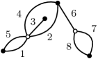
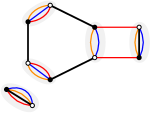
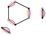
Graphical representation.
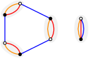
The trace-invariants can be represented as edge colored graphs.
In the mixed case we represent a tensor by a pair consisting in a white and a black vertex connected by a thick edge to which we assign a color . The input (resp. output) indices of color , (resp. ) are represented by half-edges of color connected to the black (resp. white) vertex. This is depicted in Fig. 2, on the left. In the pure case we represent a tensor as a white vertex with output half-edges , and a tensor as a black vertex with input half-edges , as depicted in Fig. 2, on the right.
The pairing of a half-edge of color on a white vertex with a half-edge of color on a black one to form an edge of color represents the identification and summation of the two corresponding indices and .
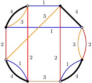
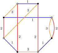
As illustrated in Fig. 3, the resulting graphs are bipartite -edge-colored graphs in the mixed case (simply colored graphs below), while in the pure case they are -colored, as there are no thick edges.
The trace-invariants are in one to one correspondence with the non-isomorphic unlabelled bipartite edge colored graphs with white and black vertices. Due to the presence of the extra edges, the invariance under relabelling in the mixed case is different from the one of the pure case.
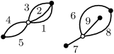
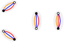
Encoding via permutations.
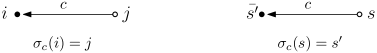
Trace-invariants are encoded by permutations. In the mixed case we label to the copies of the tensor , and we consider the permutations , obtained by setting if the output index of the tensor labeled is identified and summed with the input index of the tensor labeled . Denoting the labeled trace-invariants, we have:
| (4.2) |
In the pure case we label to the tensors and to the tensors , and we set if the output index on the white vertex is connected with the input index on the black vertex :
| (4.3) |
The summation convention is represented in Fig. 4.
Remark that if , then .
The connected components of the -edge colored graph obtained in the mixed case correspond to the blocks of the partition , and we denoted their number . This follows by observing that the cycles of the permutation correspond to the bi-colored cycles of edges with colors in the graph. We call these the mixed connected components of .
The connected components of the -edge colored graph obtained in the pure case (also called pure connected components) correspond to the blocks of the bipartite partition discussed in Sec. 2, whose number we denoted . If , we say that is purely connected.
Relabelling.
We denote for :
| (4.4) |
The trace-invariants do not depend on the labels of the tensors. The mixed and pure cases behave slightly differently:
-
•
The mixed case. In the mixed case a relabelling of the tensors corresponds to a simultaneous conjugation of all the by the same permutation , that is:
(4.5) In this case a non-labelled trace-invariant is an equivalence class (orbit in ) of labelled bipartite -edge colored graphs with the equivalence relation:
(4.6) -
•
The pure case. In the pure case the white and black vertices can be relabelled independently, that is for any :
(4.7) In this case a non-labelled trace-invariant is an equivalence class (orbit in ) of labelled bipartite -edge colored graphs (with no thick edges) with the equivalence relation:
(4.8)
Remark 4.1.
It is obvious that implies , but the converse is not true in general. What holds however is the following:
| (4.9) |
where , that is one can treat a pure invariant like a mixed one with one less color by declaring the edges of color of the pure invariant to be thick.
Matrices.
The mixed case reproduces the matrix trace invariants discussed in Sec. 3.1. Indeed, for a mixed trace-invariant is a collection of cycles with thick edges of color 2 and thin edges of color 1. Labeling the matrices corresponds to labelling the thick edges and Eq. (4.2) becomes . Relabelling the matrices corresponds to conjugating by some permutation and a non-labeled trace-invariant corresponds to the conjugacy class of of permutations of fixed cycle type.
The pure case is also matricial: one has matrices and , typically the adjoint of . A trace-invariant corresponds to a collection of alternating cycles with white and black vertices and thin edges of color 1 and 2. The invariant observables are functions of .
4.1.2 Theory of invariants
In this section, we show that asymptotically at large the trace-invariants generate the set local-unitary invariant polynomials and are linearly independent. The results we derive are weaker than the results for unitarily invariant matrices, and it should be possible to improve them. While similar results have already been obtained in the literature [59, 60, 61, 62, 63, 65, 57, 64], due to differences in vocabulary and methods we find it useful to re-derive them here.
Distance between orbits.
In the mixed case, a distance between two equivalence classes is defined by:
| (4.10) |
and it is well defined as it is independent on the particular representatives and of the classes and .
In the pure case, a distance between two equivalence classes is defined by:
| (4.11) |
which is again independent on the representatives chosen in each equivalence class.
The statement that the above functions are indeed distance functions is not trivial: in Appendix A.1 we prove the following lemma.
Lemma 4.2.
The functions and are distance functions between the equivalence classes, in particular:
and analogously for and .
A spanning family.
Let be a local-unitary invariant polynomial of degree in the tensor entries:
where the coefficients are complex numbers. Since is local-unitary invariant:
with the Haar measure on unitary matrices and using the Weingarten formula (2.11) we get:
Proceeding similarly in the pure case we establish the following lemma.
Lemma 4.3.
The trace-invariants of a tensor are a spanning family for the local-unitary invariant polynomials of degree . More precisely, for any LU-invariant polynomial of degree , there exists a set of complex coefficients such that:
where for any representative .
In the pure case, for any LU-invariant polynomial of degree in each of and , there exists a set of complex coefficients such that:
where for any representative .
Remark 4.4.
For a matrix, the statement is easily extended to polynomials of any degree using the Cayley-Hamilton Theorem. For tensors, the statement can be extended to polynomials whose degree is exponential in the system size, by application of a result by Deksen [57], see also[64], where the bound is explicitly computed for the local unitary case101010L.L. thanks Michael Walter for mentioning this fact.
Linear independence.
In what concerns the linear independence of the trace invariants, the following holds.
Theorem 4.5.
For any , there exists such that for the families of functionals below are linearly independent on :
-
•
Mixed case:
-
•
Pure case:
Proof.
The theorem is proved in Appendix A.1. ∎
Note that, in order to include all the trace invariants of degree up to , one needs to choose a larger than the number of all such invariants, which scales super exponentially with .
Scalar products between orbits.
In the course of the proof of Thm. 4.5 in the appendix we establish the following two instructive propositions.
Proposition 4.6 (Mixed case).
We consider a Ginibre random tensor, that is the components are independent complex Gaussian variables111111The joint probability measure writes . with covariance . For we define the matrix:
| (4.12) |
where is the distance between orbits in the mixed case; is the number of permutations for which and is the cardinal of the centralizer of . For large enough, the form is symmetric positive-definite and in the limit the orbits are asymptotically orthogonal:
| (4.13) |
Proposition 4.7 (Pure case).
Let be two independent Ginibre random tensors with . For the matrix:
| (4.14) |
where is the distance function in the pure case; is the number of couples of permutations for which and we denote . For large enough, the form is symmetric positive-definite, and in the limit the orbits are asymptotically orthogonal:
| (4.15) |
We have the following remark.
Remark 4.8.
In [63] a similar scalar product is considered in the pure case, but for only one Ginibre tensor , that is when and the complex conjugate, instead of the two independent ones . In order to eliminate the self contractions on , the authors introduce a “normal-ordering” of the trace-invariants:
The use of two independent tensors has the effect of precisely eliminating these self contractions without the need for normal-ordering. This small point is essentially the only difference between the complex tensor case and the bipartite distribution of two random tensors.
Non-polynomial invariants.
As grows, Lemma 4.3 and Thm. 4.5 imply that the trace-invariants are both spanning and linearity independent, hence a basis in the space of invariant polynomials. In the limit , the statement formally extends to sufficiently nice functions.
Loosely speaking, the functions we are interested in are series in the components of the tensor:
which, rescaling to with , admit a formal expansion of the form:
where for every and , is a convergent series in some neighborhood of and each is a homogeneous LU-invariant polynomial of degree . Note that the order is just the leading order in of , but can still contain some subleading dependence which washes out in the large limit. In this case there exists such that for , admits a unique expansion in trace invariants . Taking a sequence of tensors indexed by the size , for every , we assume that converges to some finite limit:
where captrues some information about at large , and for each , the series is convergent in some neighborhood of . The full expansion is usually divergent for , but for any , one has a unique convergent expansion of on asymptotic trace-invariants.
4.1.3 Finite size moments
The appropriate invariant moments for a local-unitary invariant mixed random tensor for finite are the expectations of trace-invariants [14, 15, 16, 17, 18, 19, 20, 21, 25, 26, 28, 29, 30]:
| (4.16) |
where we do not require any connectivity condition on . For a pure tensor this is replaced by with . From Lemma 4.3 and Thm. 4.5, if is a polynomial of degree in the components of , then:
| (4.17) |
and the coefficients of this expansion are unique for large enough, and similarly in the pure case. This extends to sufficiently regular invariant functions which can be obtained as the limits of sequences of polynomials, but precisely characterizing this class of functions is beyond the scope of this paper.
4.2 Finite size free cumulants
4.2.1 Linearization: intuitive picture
Our aim is to construct the equivalent of the free cumulants of random matrices discussed in Sec. 3.3 in the tensor case. In particular, the tensor free cumulants should be asymptotically linear for sums of independent random tensors.
From now on we switch notation to in the pure case to instead of . The generating functions of the moments in the mixed and pure cases are:
| (4.18) |
where and respectively and the tensors respectively are fixed sources. Note that the source terms are chosen so as to ensure that the indices of the sources and the random tensors have the same nature, for instance the indices in the first position on are contracted with the indices in the first position on etc.
From this formulas it is apparent why the pure case is not just the substitution : performing this substitution in the generating function leads to a generating function with a bi-linear source for and , which different from the generating function of the moments in the pure case which has linear sources.
Let us consider two independent LU-invariant mixed random tensors and and the two generating functions of the moments . As and are independent the generating function factors:
| (4.19) |
so that the generating function of the moments are additive:
| (4.20) |
Replacing by , differentiating times with respect to and setting to zero we have:
| (4.21) |
From the LU-invariance of the measures of and it follows that, as functions of , are LU-invariant, is LU-invariant, and the three terms in (4.21) are LU-invariant as well. Since they are homogeneous polynomials in of degree , for sufficiently large, they expand uniquely on the set of trace-invariants:
| (4.22) |
where the coefficients are explicitly computed below. Due to the linear independence, Eq (4.21) implies that are additive, as formalized in the proposition below.
Proposition 4.9.
Let and be two sufficiently regular independent random tensors, and consider coefficients for as well as defined in (4.22). Then there exists such that for any :
| (4.23) |
Everything goes through, mutatis mutandis, in the pure case:
| (4.24) |
and for two independent pairs and the cumulants are additive for any :
| (4.25) |
4.2.2 Moment-cumulant relations at finite
A trick to derive the finite versions of the free cumulants in the matrix case is to take the generating function of the classical cumulants and to average over the unitary group using Weingarten calculs. We will employ the exact same strategy to tensors and derive explicit expressions for the coefficients and . As these expressions turn out to be invertible, we posit that this coefficients yield the correct generalization of finite free cumulants to tensors.
Theorem 4.10.
Consider a mixed -invariant random tensor. Then for any fixed tensor , the Taylor coefficients of the logarithm of admit the expansion:
| (4.26) |
where the mixed finite free cumulants are (the natural generalization of (3.25)):
| (4.27) |
In the pure case, we view permutations over elements as bijections from the set of white elements to the set of black elements, and denoting the set of such bijections, we have:
| (4.28) |
where the pure free cumulants are written in terms of bipartite partitions as:
| (4.29) |
where is the restriction121212This restriction is compatible with the block, as . of the bijection to the block , and takes the labels in the set to the ones in the set , is a permutation of the elements of having the same cycle type as the permutation of the elements of , and denotes the bipartite partition into pure connected components corresponding to .
Observe that in terms of classical cumulants we have:
The equations (4.27) and (4.29) are inverted as:
| (4.30) |
where we denoted respectively the multiplicative extensions of the finite cumulants and where we recall that .
It is self evident that and are class functions for the equivalence relations respectively and regrouping the sums over into the corresponding equivalence classes and using Proposition 4.9 it follows that and are additive.
Proof.
See Appendix A.2. ∎
Note that for a purely connected we have not only (the one set bipartite partition), but also , therefore:
| (4.31) |
that is the pure cumulants can be obtained from the mixed ones by simply substituting .
4.3 Asymptotic moments
While one needs all the trace-invariants to describe unitarily invariant functions, similar to random matrices, the dominant contribution of the expectations of these quantities in the large limit should not contain more information on the asymptotic distribution than the expectations of the connected ones. This is because one expects again an asymptotic factorization of the expectations of trace-invariants over their connected components, with the non factorized parts playing a role only at sub leading orders.
4.3.1 Mixed case
We consider a mixed invariant consisting in several mixed connected components corresponding to the blocks of and we denote:
| (4.32) |
the associated finite classical cumulant. The superscript “” denotes that the components are connected in the “mixed sense”: these are the connected components of the -edge colored graph, which includes the thick edges, in representation introduced in Sec. 4.1.1.
The approach we pursue is to study invariant tensor distributions for which an asymptotic scaling function of the classical cumulants is given:
| (4.33) |
where the are non vanishing and are called asymptotic moments. The aim is to obtain a theory of (free) probability for all invariant distributions that share the same scaling function , but might have different asymptotic moments. For matrices for instance the scaling function is .
If is mixed connected, the classical cumulant equals the expectation and we have:
| (4.34) |
while if is not mixed connected, we sometimes render its connected components explicit and denote:
| (4.35) |
For we define the multiplicative extension of the asymptotic moments:
| (4.36) |
where are the mixed connected components of . We use similar notation for the finite versions , and for different ensembles , we define in the obvious manner the notations respectively and their multiplicative extensions.
4.3.2 Pure case
In the pure case, the trace invariants factor over the pure connected components, that is the connected components of the -edge colored graph described in Sec. 4.1.1. Denoting the pure connected components of corresponding to the blocks of the bipartite partition we have , and similar to the mixed case, we denote the pure classical cumulants:
| (4.37) |
We assume that a scaling function is given such that:
| (4.38) |
where the are not vanishing. If is purely connected, , then:
| (4.39) |
and if it is not we sometimes use the notation: . If is a bipartite partition such that , we define the multiplicative extension:
| (4.40) |
where , the restriction of the map to the set (which is such that ) is well defined as .
The pure case corresponds to matrices and (where can be the complex conjugate of or not). The Gaussian scaling is in this case , yielding a Wishart random matrix with asymptotic moments of order :
| (4.41) |
For , pure complex random tensor ensembles with the complex conjugate of and LU-invariant perturbed Gaussian distributions have been studied extensively [18, 21]. We review them below in Sec. 5.1 and Sec. 5.4. For such models it can be proven [21] that the classical cumulants admit an asymptotic behavior:
| (4.42) |
with . Contrary to the case, for higher the scaling factor is not necessarily additive over the pure connected components, with explicit counterexamples known for .
4.3.3 Order of dominance and asymptotic factorization
Both in the mixed and in the pure case, denoting some connected (in the appropriate sense) invariants the classical moment cumulant formula writes:
| (4.43) |
By our scaling assumption, goes to some finite value in the large limit, therefore:
-
•
all the rescaled expectations have well defined large limits if and only if the scaling function is subadditive on connected components, that is for any set of connected components :
(4.44) -
•
the rescaled expectations factor at first order:
(4.45) if and only if the scaling function is strictly subadditive, that is for any set of connected components :
(4.46)
A scaling function is clearly strictly subadditive if is additive (as it is the case for ), but because of the presence of the factor, it may very well be subadditive even if is not additive, as it is the case for .
The dominant, or first order invariants are the invariants with maximal ; the order of dominance of an invariant is the amount by which its scaling is supressed with respect to the first order ones, that is .
5 The Gaussian scaling
We discuss the scaling function for pure LU-invariant random tensors with the complex conjugate of . We first discuss the Gaussian case, when the components of are i.i.d. complex Gaussian random variables (a Ginibre like tensor) and subsequently the case of a LU-invariant perturbed Gaussian distribution. In both cases we will show that the first order asymptotic moments corresponding to invariants with maximal scaling are a subclass of the purely connected invariants, called melonic, which we will discuss in detail.
This discussion is also crucial for the rest of the paper. In Sec. 6, we will derive the first order free cumulants for generic ensembles of either pure random tensors that scale like a complex Gaussian tensor, or mixed random tensors that scale like a Wishart tensor. Due to these scaling assumption, such distributions have the same first order invariants as the pure complex Gaussian and Wishart tensors discussed here.
5.1 Asymptotic scaling of pure Gaussian tensors
We start by recalling some well-known [18] results for a Gaussian pure random tensor , that is the components of are i.i.d. complex Gaussian random variables. As shown in [18], a large class of perturbed Gaussian tensor measures fall in the same universality class. The expectation of an observables is:
| (5.1) |
where and similarly for the complex conjugate, the normalization is chosen so that , and .
We are interested in studying the asymptotic moments , which we denote from now on simply , and the scaling function , henceforth denoted . The expectations of trace-invariants are computed using Wick theorem, that is the classical moment-cumulant formula for a centered Gaussian random variable:
| (5.2) |
where defines the “Wick pairing”. Since , we get:
| (5.3) |
The classical cumulants are given by similar expressions, but with an additional connectivity condition. To be precise for a collection of purely connected trace-invariants, , denoting their disjoint union, we have:
| (5.4) |
where is the number of pure connected components of the trace-invariant defined by the permutations . This sum is dominated by the terms which minimize that is:
| (5.5) |
where:
| (5.6) |
It follows that the scaling function for a complex pure Gaussian tensor is:
| (5.7) |
We will review below various known properties of this Gaussian scaling function. However, we emphasize from the beginning that one main question remains open: it is not known wether this scaling function is subadditive or not. We conjecture this to be the case.
Conjecture 5.1.
The Gaussian scaling function:
is strictly subadditive on the connected components, that is for any with connected components for , .
5.2 Melonic and compatible invariants
Two classes of trace-invariants will play an important role in the following.
Melonic invariants.
Melonic invariants [17] dominate the asymptotic moments in the Gaussian and perturbed Gaussian cases, and more generally, in the case of pure random tensors for which the exhibit Gaussian scaling. The following definitions and results are folklore in the random tensor literature, see [21] and references therein.
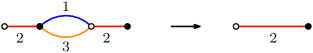
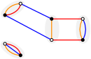
Let us fix . Melonic invariants are defined recursively in the graphical representation: the only invariant with two vertices is melonic (represented on the left in Fig. 5) and corresponds to the unique element of . If a connected trace-invariant is melonic and has more than two vertices, then it contains a black and a white vertex linked by edges, representing a tensor and a tensor sharing contracted indices. If the non contracted indices have color , replacing this pair by an edge of color as in Fig. 5, the resulting invariant is itself melonic. Fig. 6 depicts some examples of melonic graphs.131313Conversely, melonic graphs are constructed by recursive insertions of pairs of vertices connected by edges, respecting the colorings, starting from the graph with two vertices.

This recursive construction induces a pairing of the black and white vertices, corresponding to the list of pairs of vertices recursively removed. The pairing of vertices does not depend on the order in which the removals are performed: for each melonic trace-invariant this pairing is unique and will be called its canonical pairing.
An alternating cycle in the colored graph consisting in edges of a color and canonical pairs is said to be a separating cycle, if cutting any pair of edges of color in the cycle, the number of pure connected components of the graph is raised by one. An equivalent characterization of melonic invariants is that any cycle alternating edges of a fixed color and canonical pairs either contains a single colored edge, or is separating.
The following shows that among connected invariants in , melonic invariants are those which minimize the sum of distances between all the pairs of permutations .
Theorem 5.2 (Gurau, Rivasseau [14, 15, 16]).
Consider a trace-invariant . The degree of the invariant:
is a non-negative integer and for , the degree vanishes if and only if is melonic.
We have the following associated result (see e.g. [18]).
Theorem 5.3.
For , consider a trace-invariant and . Then:
| (5.8) |
with equality if and only if the trace-invariant is melonic, which implies that is melonic.
If is melonic, then there exists a unique such that and : it corresponds to the canonical pairing of . This holds in particular if is melonic and purely connected.
If is melonic but not purely connected, there are other (different from the canonical pairing) such that and .
Compatible invariants.
Compatible invariants (see e.g. [55]) are those for which there exists a permutation lying on a geodesic linking every pair of permutations of . Defining:
| (5.9) |
then vanishes if and only if is compatible and if , we say that renders compatible.
Lemma 5.4.
Melonic invariants are compatible. If is melonic, there is a unique permutation which realizes , and it corresponds to the canonical pairing of .
5.3 Order of dominance for the Gaussian scaling
Rewriting the Gaussian scaling function in using Thm. 5.3 we conclude that the finite cumulants scale like:
| (5.12) |
where the minimum is taken over the such that and is the number of with which minimize .
First order invariants.
The first order contributions are the invariants with maximal scaling.
Theorem 5.5.
For and the order complex pure Gaussian tensor the invariants with maximal scaling are the purely connected, melonic invariants. Furthermore, the corresponding asymptotic moment is one, and the first correction is of order :
The only point not contained in Thm. 5.3 is the order of the correction, see e.g. [24]. The fact that is to be compared with the case (4.41), for which one obtains the Catalan number . The melonic invariants can be enumerated and the number of connected melonic invariants is the Fuss-Catalan number [17], which is to be compared with the case for which there is only one such invariant at each .
Purely connected invariants.
The order of dominance of an invariant captures the amount by which its scaling is suppressed with respect to the leading order invariants. The invariants of orders are purely connected and such that . For order and above, both and play a role in determining the order. This is new with respect to the case, where there is no equivalent of .
For purely connected trace-invariants, (5.12) simplifies to:
| (5.13) |
and one can in principle [22, 30] identify for any order the purely connected trace-invariants with . The contributions of order 2 and 3 are for instance given in (19) and (25), (26) and (27) of [22] and are asymptotically enumerated in [23]. In practice, this becomes rapidly quite tedious. Given a purely connected trace-invariant , short of a full computation, it is not obvious how to relate to the properties of .
Proposition 5.6.
From Eq. (5.11) it follows that for purely connected we have:
with equality if and only if is compatible.
This bound is useful when it is saturated, that is for compatible invariants. However this is of limited interest as for every it is easy to construct both compatible and non-compatible invariants satisfying .141414This relies on the method of [24]. One can also prove that the probability for an invariant of degree to be compatible tends to one when goes to infinity.
Non-connected invariants.
The first contribution with arises at order and corresponds to consisting of two purely connected melonic graphs. This generalizes to arbitrary number of connected components.
Theorem 5.7.
For and the order complex pure Gaussian tensor, the invariants with maximal scaling at fixed number of connected components are the disjoint unions of melonic purely connected components:
where is the number of such that is melonic.151515It should be straightforward to enumerate this family.
For non-melonic, non-connected invariants, the situation is worse. The task of computing the Gaussian scaling function for an arbitrary invariant is computationally hard: beyond checking all the Wick contractions, no procedure is known to read off or to construct the minimizing under the constraint . As general exact results are lacking, the best one can do is to search for convenient bounds on the scaling function. For any invariant an obvious bound on the Gaussian scaling is:
| (5.14) |
The bound is saturated by the melonic family and is additive on the connected components.
The whole idea is to try to improve this naive bound as much as possible. The strategy is to search for bounds consisting in a constant term , the scaling of the expectation of , plus a piece which is additive on the connected components. The whole point is to find optimal upper bounds: for various families of connected invariants one searches for some numbers for such that:
| (5.15) |
and the bound is tight,161616It is immediate to prove that if such a bound holds and it is saturated for all the connected invariants then the scaling is strictly subadditive. that is for any , there exists some with such that the bound is saturated for . Of course this always works for , and the point is to improve this by increasing as much as possible: while for purely connected melonic invariants can not be improved, it turns out that for other invariants this can be improved to some [25, 26, 27, 28, 29, 30, 31].
For , the maximal allowed by the scaling of the connected invariants, , works in all the examples treated so far.171717Rigorously, one should denote this , as one proves the bound for a fixed family of invariants. It is an open question wether these improved bounds change by including more invariants. However, as detailed in the last section of [30] this can not be true in general. For there exists a connected such that but , inconsistent with this choice of . In particular:
which is less suppressed that what the intuition from measure concentration estimates would suggest [56]. To our knowledge this counter-intuitive scaling is specific to the tensor realm. However, we stress that the Gaussian scaling function is clearly subadditive in this case, that is this example does not contradict our conjecture 5.1.
5.4 Random tensor models with invariant potentials
The expectations of a perturbed Gaussian tensor measure are given by:
| (5.16) |
where the perturbation potential is an invariant:
with a choice of scaling, suitable combinatorial factors and the coupling constants. The convergence of the integral is ensured for some choices of the couplings. We denote the (potentially infinite) set of trace-invariants for which . The Gaussian case is recovered by setting all the couplings to , and will be denoted in this subsection.
The characterization of the asymptotic moments of such distributions is usually approached “perturbatively”, that is by expanding in Taylor series end exchanging the Gaussian integral and the sum. The cumulants are then expressed as divergent sums over connected -colored graphs. The limit selects sub-series of graphs that optimize some combinatorial constraints and are summable when the coupling constants are sufficiently small. The fact that this procedure provides the true large asymptotic of the cumulants of (5.16) is proved by constructive methods [18, 33, 21].
The advantage of the perturbative approach is that it reduces the computation of the asymptotic scaling of the cumulants for distributed as in (5.16), to the evaluation of the asymptotic scaling of Gaussian cumulants of the form:
| (5.17) |
where is the order pure Gaussian tensor of the previous subsections, and the can be any invariant in .
Denoting the disjoint unions of the respectively the , the total number of tensors , such that , and and arbitrary permutation, the asymptotic scaling of is obtained (5.5) by maximizing over such that . As discussed in the previous section, a bound of the type (5.15) on the Gaussian scaling always holds, at least for . Optimizing this bound on all the possible , which is at least in principle possible, the scaling of is:181818Strictly speaking this is just an upper bound, as it might happen that, although optimal, the scaling bound is not saturated by the particular configuration of s which maximize the right hand side.
| (5.18) |
where we call the optimized optimal.
The statements in the theorem below are either reformulations of the results in [18], or follow from Eq. (5.18).
Theorem 5.8 (Gaussian universality).
As a function of the scaling of the potential in the distribution (5.16), we obtain different large limits:
-
•
If for all the invariants , then the distribution is asymptotically Gaussian with a modified covariance [18]:191919The non trivial part in [18] is the use of the in the Gaussian scaling function, which is not captured by (5.18).
(5.19) where the notation signifies that the two are identical at leading order in the large limit. Furthermore, denoting the cardinal of the set on which acts, is the unique power series solution of the equation:
(5.20) We stress this hold independently on wether the bound on scaling can be optimized or not. The same holds if for the melonic graphs and for the non melonic ones.
Assuming the bound on scaling can be optimized and (5.18) holds for some optimal for the non melonic , then:
-
•
If for all , ,202020For instance if for all , . then the distribution is asymptotically Gaussian identical with the distribution of , in the sense that for any trace-invariant :
(5.21) - •
- •
-
•
If for some , , then the distribution does not admit a large limit.
5.5 Scaling of the Wishart tensor
Similar to a Wishart matrix, the Wishart tensor is obtained from the pure complex Gaussian tensor partially tracing over one of its indices:
| (5.22) |
A priori this is just an equivalent perspective on the pure case with the difference that there is a fixed labelling of the and indicating the pairs whose th indices are contracted to form a mixed tensor.
Scaling function.
As is a pure complex Gaussian, we have for :
| (5.23) |
where the minimum is taken over for which , and so that . As with the Gaussian scaling in (5.7) we have:
| (5.24) |
First order.
The first order corresponds to the which are mixed connected (hence not necessarily purely connected) and for which is melonic, that is they are melonic when including the thick edges corresponding to the permutation , therefore:
-
If is purely connected, then its canonical pairing must be the identity: .
-
If is not purely connected, then each of its pure connected components is melonic the thick edges either connect canonical pairs in the same connected component or, alternating with canonical pairs, form separating cycles in .
This is just a partition of the melonic connected graphs with colors into two classes, according to the effect the deletion of all the edges of color has on the graph: either the deletion of these edges does not disconnect the graph, or it does disconnect it into a union of melonic connected components.
6 Free cumulants of unitarily invariant random tensors
In this section, we define and discuss first order free cumulants in two situations: pure random tensors that scale like a pure complex Gaussian, and mixed random tensors that scale like a Wishart tensor.
6.1 Free cumulants for pure Gaussian tensors
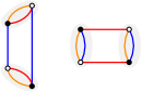
We strart from the example of a pure complex Gaussian tensor with covariance . One then has for the two-tensors invariant (left of Fig. 5), the only element of , which we denote by :
| (6.1) |
so that the asymptotic covariance is:
| (6.2) |
In the case discussed in Thm. 5.8 of an asymptotically Gaussian random tensor model for instance, one would have .
Free cumulants.
In the Gaussian case the generating function of the moments ca be directly computed:
| (6.3) |
hence the only finite free cumulant is , and the only non trivial asymptotic free cumulant is:
| (6.4) |
The free cumulants asymptotic moments relation is then and Eq. (5.6) gives its inverse, that is the asymptotic moments free cumulants relation:
| (6.5) |
In particular, for if is purely connected and melonic the cardinal is just , see Thm. 5.5, therefore one has:
| (6.6) |
Remark 6.1.
This is to be compared with the result, when (6.4) still holds, but for with , the number of which minimize is the Catalan number (2.4):
| (6.7) |
The notion of cumulant depends on whether we consider a pure complex tensor with , or a (mixed) Wishart matrix in . The cumulants in the two cases are related by:
| (6.8) |
which agree since the pure connected components of are a collection of invariants in . More generally .
6.2 Free cumulants for pure unitarily invariant random tensors
We aim to identify the corresct notion of free-cumulants associated to the first order moments for LU-invariant pure random tensors whose classical cumulants scale with the Gaussian scaling function (5.5), that is:
| (6.9) |
We do not assume anything regarding the asymptotic moments : they are an unspecified list of numbers that characterize the distribution asymptotically. This includes the pure complex Gaussian case and some Gaussian measures perturbed by invariant potentials, but the results derived here are a priori more general.
Our starting point is Theorem 4.10, namely the formula of the finite free cumulant:
| (6.10) |
supplemented by the finite moment cumulant expressions for :
| (6.11) |
and the asymptotic of the Weingarten function for .
Limit of first order finite free-cumulants.
As discussed in Section 5.3, the first order consists of the purely connected melonic trace-invariants.
In order to state the appropriate moment cumulant relation at first order, we recall that means that for all , , that is, for each cycle of , the restriction of to the support of this cycle is a non-crossing permutation. Also, for , we define , where is the Möbius function on the lattice of non-crossing partitions. Denoting the lattice of non-crossing partitions on elements, is the Möbius function on the direct product of lattices , which is itself a lattice.
Theorem 6.2.
Let and let be a melonic purely connected invariant, , and let be the permutation defined by the canonical pairs of . Consider a pure random tensor whose classical cumulants scale as in Eq. (6.9). Then the finite free-cumulant scales as and:
| (6.12) |
In particular the s in the sum are melonic, but not necessarily purely connected and is the canonical pairing on .
Proof.
The proof is presented in Sec. B.1. ∎
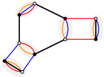
In order to gain some intuition on the s contributing to this sum, we consider a melonic graph with canonical pairing given by the identity212121The graph in the previous theorem.. Then for any color the permutation consists of either fixed points or cycles of length and can at most split some cycles of length 2 into fixed points. It follows that the graphs are obtained from by choosing pairs of edges of the same color incident to canonical pairs and flip them, that is disconnect the two edges in the pair and reconnect them in the only possible configuration different from the original one. See Fig. 7
The theorem generalizes trivially for pure random tensors. Let us revert to the notation instead of . We consider some pure random tensors , and so on with bipartite joint distribution and we denote with and and with . For and , we define:
| (6.13) |
where collects the labels of the white vertices, and the ones of the black vertices. We denote the appropriate generalization of the pure cumulants in (4.29) to pairs of tensors and assuming that the generalized scaling ansatz:
| (6.14) |
holds, then Theorem 6.2 goes through, thus defining . If for all and , and are drawn independently from a set of complex pairs (or a bipartite distribution), then define the joint distribution of the pairs.
Note that using pure cumulants with pairs , as we do here, or mixed cumulants with substitutions in these scaling assumptions leads to different results as in the second case one considers only trace invariants in which the tensors on the vertices and belong to the same pair. To clarify this point, consider the invariant consisting in the disjoint union of two fundamental melons and two pairs and then:
-
•
with pure invariants (as we chose to do here) one makes scaling assumptions on the four combinations:
-
•
with mixed invariants, but substituting one only obtains the two combinations:
Asymptotic additivity.
We have so far only considered pure cumulants and pure random tensors, and therefore we dropped the index on the cumulants. For the purposes of the next proposition we, will reinstate it, in order to differentiate them from the mixed cumulants which are obtained as the large limits of the mixed finite free cumulants in Theorem 4.10.
Let and be two independent LU-invariant pure random tensors satisfying (6.9) and we assume that (6.14) holds for drawn from and drawn from . This assumption holds for classical random matrix ensembles, and for instance for pure Gaussian tensors. In that case, the scaling is satruated if among the Wick contractions at leading order there exist some such that for all , and are all of the same type or , and if not the moment is supressed in scaling.
Theorem 6.3.
Let , be melonic , purely connected , and labeled such that its canonical pairing is . Let and be two independent LU-invariant pure random tensors satisfying (6.14), and define . Then is a mixed tensor, and consequently one can consider the finite free cumulants:
| (6.15) |
With the scaling assumptions (6.14), the mixed free cumulant at large exists:
and at large the state purifies, that is:
| (6.16) |
Proof.
The theorem is proven in Sec. B.2. ∎
In this proposition we distinguish between the pure and the mixed cumulants, notably on the left and right hand side of the Equation (6.16). However, as shown in Eq. (4.31) for the purely connected invariants the mixed cumulant for and tensor product tensor is equal to the pure cumulant for the pair and this holds at finite :
| (6.17) |
Properties of first order free cumulants.
Free-cumulants for arbitrary melonic invariants are defined as multiplicative extensions. The following theorem (proven in Sec. B.3) is analogous to Prop. 11.4 of [2].
Theorem 6.4.
Let be a melonic trace-invariant () and be the permutation defined by the canonical pairs. We denote its pure connected components and we define:
| (6.18) |
where . Then:
-
•
Each is itself melonic, with the same canonical pairing as .
-
•
The family is the multiplicative extension of the family defined in Theorem 6.2 :
(6.19) - •
For a Gaussian complex tensor we have and, setting , the only non-zero term in the sum (6.20) is , the -uplet of permutations (the melonic invariant consisting of disjoint two-vertex graphs with canonical pairing is the identity), that is:
| (6.21) |
and one recovers (6.7).
For the free cumulants of the square Wishart random matrix (3.18) are , and those of the GUE random matrix are . Both lead to similar combinatorics, in the sense that the associated asymptotic moments enumerate graphs embedded on the 2-sphere in the same combinatorial universality classes. For the pure case treated here this is no longer the case: as explained above, choosing for purely connected melonic invariants leads to richer combinatorics (6.20) in comparison to the choice , which leads to (6.21).
6.3 A first glimpse at purely connected higher orders
Non-melonic purely connected invariants are higher-order free cumulants as they are more suppressed that their melonic counterparts in the large limit. This is new with respect to matrices, for which the order of dominance is given only by the number of pure connected components.
In the proof of Theorem 6.2 we have obtained (see Eq. B.4 and subsequent) the general formula for a finite free cumulant associated to a purely connected invariant:
| (6.23) |
where . Furthermore, we have shown that if and only if:
| (6.24) |
and that , that is the condition is always satisfied at least for . We denote the set of terms contributing to leading order by:
| (6.25) |
Proposition 6.5.
Let , , be purely connected. Consider a pure random tensor whose cumulants scale as (6.9). Then the finite free-cumulant scales as , where , and:
| (6.26) |
We note that if there exists a for which both and , that is , then , and in this case the cumulant is a sum over a lattice and the relation can be inverted using Möbius inversion. However, at this point, it is not clear if such a permutation always exist, or how to organize as a lattice in general.
The condition (6.24) can be writted in a form addapted to compatible invariants discussed in Section 5.2. We first reformulate the Equation (5.10) as:
| (6.27) |
On the other hand, we define:
| (6.28) |
and with the help of these two relations we express:222222We used .
| (6.29) |
We conclude that the set is also the set of pairs such that and:
| (6.30) |
Assuming that is compatible, this condition becomes . On the other hand, we also have that if , then renders compatible if and only if it renders compatible and moreover it is such that .
This allows defining equivalently as the set of pairs such that and there exists which renders compatible and it is such that . At this point, in order to proceed, we would need to determine whether it is possible for a to contribute to the leading order. We posit that this is not the case.
Conjecture 6.6.
Consider . Then any satisfying is such that , that is, .
It is straightforward to prove that if the Gaussian scaling is subadditive then this conjecture holds, that is Conjecture 5.1 implies the present conjecture.
Assuming this conjecture,232323And assuming that if several permutations render compatible then the families of invariants such that are disjoint, which is a weak assumption view that one expects usually at most one such to exist. then the cumulants of purely connected invariants in Proposition 6.5 become for compatible:
| (6.31) |
This is a sum which can be inverted. In particular, if there is a unique such that then, choosing the labelling of so that this is the identity, we have:
| (6.32) |
6.4 Random tensors that scale like a Wishart tensor
In this section, we will discuss the case when our random tensor is mixed rather than pure. As scaling assumption, we will consider mixed random tensors that scales like the square Wishart random tensor of Section 5.5, that is we assume that for :
| (6.34) |
where the minimum is taken over for which . Note that and also with the Gaussian scaling function in (5.7).
For the version of the theorem that involves different tensors, one must make the following stronger assumption for any :
| (6.35) |
This includes the case where there exists a LU-invariant pure random tensor with indices, not necessarily the pure complex Gaussian itself, but displaying Gaussian scaling (6.9), and is:
| (6.36) |
For this case the results discussed here are to be compared to the pure case with one additional color (see Sec. 5.5), and we review this comparison at the end of this subsection.
For the general case of a mixed tensor with scaling function , the thick edges cannot a priori be seen simpliy as an additional color. In order to understand this, let us first study the free moment-cumulant relations for the first order moments , corresponding to a melonic connected invariant such that is melonic.
Theorem 6.8.
Let be connected and such that (which implies that is melonic) and let be the canonical pairing of . Consider some mixed random tensors that scale as in (6.34), and satisfy (6.35). Then the limit of the mixed finite free cumulant associated to is:
| (6.37) |
and the in the sum are such that , with canonical pairing . Furthermore:
- •
-
•
The relation can be inverted. With the notations above:
(6.38)
Proof.
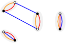
The proof can be found Section B.4. ∎
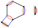
In the general mixed case one cannot treat the thick edges (the identity) as an additional color because the inverse relation (6.38) does not include a sum over permutations such that , as one would have in the pure case with one additional color. See the examples in Fig. 8
The inverse relation (6.38) simplifies if the connected components of are purely connected, as it is that case if the canonical pairing on is , to:
| (6.39) |
that is one recovers the formula from the pure case with indices with canonical pairing (6.20). Thus for the purely-connected melonic invariants, which are first order in both situations, nothing distinguishes a pure distribution with indices with Gaussian scaling function from a mixed distribution with scaling function . The difference between the two comes from fact that there are more first order invariants in the mixed case, namely those which are connected but not purely connected
Observe that there are observables for which forces . This is for instance the case for melonic with all equal. For such observables the asymptotic moment equals the free cumulant, and it is additive. This phenomenon is specific to the tensor case and does not arise for matrices.
If for the first order (connected and melonic) and we pick a connected melonic invariant such that its the canonical pairing is is the identity (in which case is purely connected) that is given by the same product of Catalan numbers as in Equation (6.22).
Higher orders.
Mixed perspective on the pure case.
For the genuine Wishart like case, we have the following.
Proposition 6.9.
Let for some pure random tensor with indices with Gaussian scaling (6.9). Let be such that is melonic with canonical pairing of . Then the pure cumulants of and the mixed cumulant of are related by:
| (6.41) |
where the permutation encodes a change of the thick edges representing the tensors .242424If we change variable to corresponding to a change of labeling of the black vertices, the identity after the change of variables represent the thick edges, but before this change of labeling, the thick edges are represented by the permutation . Conversely:
| (6.42) |
If is purely connected, and .
Proof.
See Section B.5. ∎
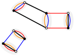


In particular, if is a pure Gaussian for and is as in (6.36), we have from (6.4) with , that which is zero unless has only two vertices, in which case it is one. Inserting this into (6.42) for satisfying melonic, we see that the right-hand side is zero unless , and hence , which is different from the case of a pure complex Gaussian random matrix and Wishart matrix (6.8).
6.5 Asymptotic tensor freeness at the level of free cumulants
We will say that a family of random tensors are asymptotically free, if and only if the free cumulants that involve at least two different tensors from this set vanish.
The asymptotic tensor freeness (or asymptotic first order tensor freeness) of a collection of random tensors can be formulated as the fact that for any first order , the involving different tensors vanish.
-
•
For mixed tensors that scale like the tensor Wishart (6.34) and (6.35), the first order consists of the connected , such that . This constrains the thick edges as follows: in the graph , any cycle of alternated thick edges and canonical pairs that involves more than one thick edge must be separating. are asymptotically free if for any such and any with :
(6.43) whenever for some .
-
•
For pure tensors, , , , that scale like a complex Gaussian (6.9) and (6.14), the first order consists of the purely connected and melonic . We require that be labelled such that its canonical pairing is the identity and consider for , and with and . Note that we allow , that is one could have and . In that case, , , are asymptotically free if:
(6.44) whenever or , or for some .
In the pure case, if there exists such that for each , , then by changing the labeling of the black vertices one may replace by , setting with now defining the canonical pairing . After this change of labeling, the black and white vertices represent the inputs and the outputs of the same pure tensor , and are linked by a thick edge encoded by the permutation .
If this holds, the vanishing condition for purely connected with canonical pairing the identity (i.e. with ) must be considered in both the pure and mixed cases.
On the other hand, the vanishing condition in the pure case when this does not hold must be considered only in the pure case, while the vanishing condition for such that , connected but not purely connected, must be considered only in the mixed case.
Appendix A Proofs of Sec. 4
We gather here the proofs of statements in Sec. 4.
A.1 Proofs of Sec. 4.1.2
Proof of Lemma 4.2:
The two posited distance functions are class functions, hence well defined. They are clearly non negative, symmetric and respect the triangle inequality. For instance, for any and any we have and we take the minimum first over and then over .
It remains to prove that if then (the reciprocal is trivial). From the triangle inequality, for any :
therefore if we have that for all , and there exists an such that either or for each . Note that in principle we could have for , but for some .
However, the bipartite map has the same number of and vertices and every connected component of this map has either only one or only one vertex. It follows that each connected component of this map must have exactly one and one vertex and be planar, that is either , or , therefore . The proof for is similar. ∎
Proof of Thm. 4.5:
We start by proving the linear independence in the mixed case. We consider the family of trace invariants with with , a set of corresponding complex numbers , and the linear combination:
But then trivially, if is a complex random tensor with finite moments, this implies:
| (A.1) |
and in order to conclude it is enough to exhibit a particular random tensor such that the covariance matrix:
is invertible for large enough. Let us take distributed according to the Ginibre ensemble, that is the components are independent complex Gaussians with covariance . The only non zero elements of the covariance matrix are obtained from the Wick theorem as:
| (A.2) |
where the permutation encodes the Wick pairings between s and s. In terms of the distance function in Eq. (4.10) this becomes:
where is the number of for which the distance is attained. Since , the diagonal terms are strictly positive are of order , while the off-diagonal terms are all suppressed in , as for any two different classes. The following lemma completes the proof.
Lemma A.1.
Let be a Hermitian matrix with positive diagonal entries . If , then is positive definite and invertible
Proof.
Without loss of generality, we may assume that the matrix has diagonal entries equal to one (otherwise we multiply on the left and on the right by ) and off-diagonal entries bounded as . We split , where has null diagonal and operator-norm less than : as the latter is bounded by the Frobenius norm, , therefore is positive-definite and , where the series converges in operator norm. ∎
The proof is similar in the pure case, choosing and to be independent, distributed on complex Gaussians with covariances and evaluating the covariance matrix:
| (A.3) |
where is the number of for which the distance is attained. ∎
A.2 Proof of Thm. 4.10
In the mixed case, due to the -invariance of , we can write in terms of the tensor HCIZ integral [5, 6]. Denoting with and , where denotes the Haar measure on , from the moment-cumulant relation (2.8) we have:
The integral over the unitary group is computed from Eq. (2.11):
As factors over the mixed connected components in and the summand is invariant under relabellings, we can exchange the sum over partitions with the ones over permutations to obtain:
In the pure case, similar manipulations lead to the similar formulae, but with the “mixed” replaced by “pure”. In detail, we start from:
and we integrate over the unitary group. In this context, it is convenient to regard the permutations in Eq. (2.11) as bijective mappings from the white elements to the black ones, that is . Denoting the set of bijections from the elements of to the ones of we have:
and we observe that is a permutation of the black elements having the same cycle type as the permutation of the white ones. The invariants now factor over the pure connected components, and when commuting the sum over with the ones over and , the compatibility condition that correspond to the parts of implies that must be coarser that the partitions in pure connected components and , leading to:
In order to invert the relations we start by averaging the expectations over the unitary group:
which is, using the definition (4.2) of the trace-invariants and Eq. (2.11):
where again in the pure case the sum should be considered as a sum over bijections between the white and the black vertices. Recalling that , this is:
and similarly for the pure case. We define the multiplicative extension in the mixed case:
| (A.4) |
while in the pure case we have and . Comapring with (4.27) leads to:
| (A.5) |
where the last equality follows by Möebius inversion. The pure case is similar. ∎
Appendix B Proofs of Sec. 6
B.1 Proof of Thm. 6.2
General asymptotic.
The finite free cumulants in Theorem 6.2 simplify for a purely connected , as the sum over partitions reduces to one term corresponding to the one set partition. Expressing it in terms of classical cumulants we have:
| (B.1) |
where all the partitions encounterd in this proof are bipartite, and all the permutations should be sees as mapping white to black vertices.
The Gaussian scaling hypothesis (6.9) yields:
| (B.2) |
where each minimum is taken over the with . We denote
the sets of permutations over which the minimum in the Gaussian scaling is taken, that is:
| (B.3) |
Taking into account that asymptotically the Weingarten functions behave as:
we obtain the large asymptotic behaviour of the finite free cumulant:
| (B.4) |
where . Now, for any , one has the -fold triangular inequality:
| (B.5) |
with equality if and only if . It follows that and at leading large order, , only the couples belonging to the set:
| (B.6) |
contribute to the cumulant. Note that this set is nonempty, as for we have .
Expressions in terms of degrees.
In order to use our results on the degree of graphs, it is convenient to parametrize the set using the degree form Theorem 5.3. For , and , as the restriction of to each block of is connected, we have and:
| (B.7) |
At the same time, we also have the following.
Lemma B.1.
For any we have:
| (B.8) |
Proof.
Consider the colored graph . Deleting an edge in each cycle does not disconnect the graph. Deleting the remaining edges in lead to the graph , and the number of connected components can not increase by more than for each of these edges. ∎
The -fold triangular inequality (B.5) is expressed equivalently for any , , and as:
| (B.9) |
hence the condition defining the set becomes in terms of the degree:
| (B.10) |
The melonic case.
If is simply connected and melonic, and , then from Theorem 5.3, for there exists a unique such that , and (B.10) simplifies to:
| (B.11) |
and since all the three terms are non-negative, this implies , , and . The last condition tels us that must be melonic, but not necessarily purely connected.
From (B.9), for any with we have that for any :
| (B.12) |
with equality if and only if . Let such that : then , and as is purely connected, is the canonical pairing of , and .
Reciprocally, if is melonic purely connected and is its canonical pairing and if is such that , then for one has and from (B.9):
| (B.13) |
It follows that , that is, or said otherwise, , and on the other hand , hence and in particular is melonic.
B.2 Proof of Thm. 6.3
Asymptotic scaling of the sum.
The first statement that needs to be proven is that, with the scaling hypothesis (6.9), the finit cumulants of admit a large limit:
| (B.15) |
Using the multilinearity of the trace-invariants, one has for the purely connected components of :
| (B.16) |
and due to the multilinearity of the classical cumulants we obtain:
| (B.17) |
From the assumption (6.14) we have that at large :
Limit of mixed invariant tensors that scale like a pure Gaussian.
The starting point is now:
| (B.18) |
where the difference with (B.4) lies in the fact that . Following the same steps as in Sec. B.1, we decompose the exponent in the same way, with an additional term . This brings the additional condition , or equivalently . Having imposed the labeling of to be such that its canonical pairing is the identity, is satisfied for any , as the canonical pairing on is also the identity. The rest of the reasoning is similar to Sec. B.1. The additivity (purification) is just a consequence of the additivity of pure finite free cumulants.
B.3 Proof of Thm. 6.4
The first assertion has been proven in Theorem 6.2
Multiplicativity.
Inversion.
If all the tensors are identical, the inversion is an example of Möbius inversion. Without loss of generality we set . The direct product of copies of the lattice of non crossing partitions is the lattice whose Möbius function is (Prop. 10.14 of [2]), and we recall that is isomorphic to the lattice of non crossing permutations on , , for any cycle with elements.
Here for each we fix some with elements for which , and we work in the lattice product , which contains . Any interval where is itself a lattice (Remark 9.26 in [2]). In particular, letting be melonic and with canonical pairing the identity, and be the -uplet of permutations , that is the melonic invariant consisting in disjoint two-vertex graphs with canonical pairing the identity, the Möbius inversion (Proposition 10.6 in [2]) ensures that (6.18) can be inverted on the interval , hence for any :
| (B.19) |
and in particular this holds for .
We now turn to the case when the tensors are not identical: we take and and we consider:
for melonic (not necessarily connected) with canonical pairing . We posit that the inverse relations are , and we verify by substitution:
| (B.20) | ||||
| (B.21) |
and summing the Möbius function of a lattice gives the delta function (see Remark 10.7 of [2]), hence the last sum is .252525 Setting , and the sum becomes which factors over . Reciprocally:
| (B.22) | ||||
| (B.23) |
B.4 Proof of Thm. 6.8.
The proof follows the one in the pure case presented in Section B.1 by replacing with and observing that the pure connected components of are one to one with the mixed connected components of , thus:
where for , .
General asymptotics.
The -fold triangular inequality (B.5) is now replaced with:
| (B.24) |
with equality if and only if , that is , and the leading order contributions satisfy:
| (B.25) |
which is saturated at least , hence for a connected , scales as .
First order.
Using the degree, the Eq. (B.7) gives rise to a term instead of , and applying Lemma B.1 to and we get:
| (B.26) |
where for connected, and (B.24) is equivalent to:
| (B.27) |
The rest follows as in Sec. B.1, identifying for connected such that is melonic, the set of satisfying (B.25) as and , where is the canonical pairing of .
The additivity follows from the additivity of the finite free cumulants.
Inversion.
The inversion is slightly more involved. We start from the multiplicative extension to any non-necessarily connected such that with canonical pairing :
| (B.28) |
where . Changing variables for and , we rewrite this as:
| (B.29) |
where the notation indicates that after the change of variable, the variable is now associated to the thick edge going from the white vertex to the black vertex . After this change of variable, which corresponds to a relabelling of the black vertices to set the canonical pairing to the identity, one has , , and similarly for . For we denote:
| (B.30) |
We fix a connected with and consider the relations above for all the such that : the are not necessarily connected and satisfy . We rewrite (B.29) for any as:
| (B.31) |
which holds as in the lattice interval we have and . Note that is a sublattice of , and we ca invert this formula (Proposition 10.6 in [2]) to obtain for all :
| (B.32) |
and again forces . Retracing our steps we conclude.
B.5 Proof of Prop. 6.9
Starting from the free moment-cumulant formula for the pure case:
| (B.33) |
we use the invariance and observe that:
| (B.34) |
The invariant is such that is melonic, with canonical pairing , so that:
| (B.35) |
Changing back to and and putting the two relations together, we have:
One has to be careful that for and , the identity is the permutation encoding the thick edges and the canonical pairing is , but after the change of labeling the permutation encoding the thick edges is , and the canonical pairing is . As , factors over the connected components of , exchanging the sums over and , we get:
and the last sum is , so that setting , we get:
| (B.36) |
Reciprocally, starting from the mixed moments in terms of the pure ones which we express in terms of pure cumulants, and substituting into the mixed cumulant moment formula we get:
| (B.37) |
and exchanging the summations and summing the Möebius functions we find:
| (B.38) |
References
- [1] P. Biane, “Some properties of crossings and partitions”, Discrete Mathematics 175 (1997), 41–53.
- [2] A. Nica and R. Speicher, “Lectures on the combinatorics of free probability," volume 13. Cambridge University Press, 2006.
- [3] R. Speicher, “Multiplicative functions on the lattice of non-crossing partitions and free convolution”, Mathematische Annalen 298 (1994), 611–628.
- [4] D. Voiculescu, “A strengthened asymptotic freeness result for random matrices with applications to free entropy” International Mathematics Research Notices, Volume 1998, Issue 1, 1998, Pages 41–63.
- [5] B. Collins, R. Gurau, L. Lionni, “The tensor Harish-Chandra–Itzykson–Zuber integral I: Weingarten calculus and a generalization of monotone Hurwitz numbers”, accepted for publication in J. Eur. Math. Soc. (JEMS), [arXiv:2010.13661].
- [6] B. Collins, R. Gurau, L. Lionni, “The tensor Harish-Chandra–Itzykson–Zuber integral II: detecting entanglement in large quantum systems”, [arXiv:2201.12778].
- [7] B. Collins, J.A. Mingo, P. Śniady, R. Speicher, “Second Order Freeness and Fluctuations of Random Matrices, III. Higher order freeness and free cumulants”, Documenta Mathematica 12 (2007) 1-70, [arXiv:math/0606431].
- [8] D. Weingarten, “Asymptotic behavior of group integrals in the limit of infinite rank,” Journal of Mathematical Physics 19, 999 (1978).
- [9] B. Collins, P. Śniady, “Integration with Respect to the Haar Measure on Unitary, Orthogonal and Symplectic Group,” Commun. Math. Phys. 264, 773-795 (2006), [arXiv:math-ph/0402073].
- [10] S. Dartois, L. Lionni, I. Nechita, “On the joint distribution of the marginals of multipartite random quantum states”, Random Matrices: Theory and Applications, 9(03):2050010, 2020 [arXiv :1808.08554].
- [11] L. Lionni, “From higher order free cumulants to non-separable hypermaps”, [arXiv:2212.14885].
- [12] B. Collins, “Moments and Cumulants of Polynomial random variables on unitary groups, the Itzykson Zuber integral and free probability”, Int. Math. Res. Not. 2003(17), 953-982 (2003).
- [13] J. Mingo and R. Speicher, “Second Order Freeness and Fluctuations of Random Matrices: I. Gaussian and Wishart matrices and Cyclic Fock spaces”. J. Funct. Anal., 235, 2006, pp. 226-270.
- [14] R. Gurau, “The expansion of colored tensor models”, Annales Henri Poincaré 12:829-847, 2011.
- [15] R. Gurau, V. Rivasseau, “The expansion of colored tensor models in arbitrary dimension”, Europhys. Lett. 95:50004, 2011.
- [16] R. Gurau, “The Complete Expansion of Colored Tensor Models in Arbitrary Dimension”, Ann. Henri Poincaré 13, 399–423 (2012).
- [17] V. Bonzom, R. Gurau, A. Riello, V. Rivasseau, “Critical behavior of colored tensor models in the large limit”, Nucl. Phys. B853 (2011) 174-195.
- [18] R. Gurau,“Universality for random tensors”, Annales de l’I.H.P. Probabilités et statistiques 50.4 (2014): 1474-1525.
- [19] V. Bonzom, R. Gurau, and V. Rivasseau, “Random tensor models in the large limit: Uncoloring the colored tensor models”, Physical Review D, 85:084037, 2012.
- [20] V. Bonzom, “Revisiting random tensor models at large via the Schwinger-Dyson equations”, J. High Energ. Phys. 2013, 160 (2013).
- [21] R, Gurau, “Random Tensors”, Oxford University Press, 2016.
- [22] V. Bonzom, L. Lionni, and A. Tanasa, “Diagrammatics of a colored SYK model and of an SYK-like tensor model, leading and next-to-leading orders”, J. Math. Phys., 58:052301, 2017.
- [23] E. Fusy, L. Lionni, and A. Tanasa, “Combinatorial study of graphs arising from the Sachdev-Ye-Kitaev model”, European Journal of Combinatorics, Volume 86, May 2020, 103066, arXiv:1810.02146 [math.CO], 2018.
- [24] R. Gurau, G. Schaeffer, “Regular colored graphs of positive degree”, Ann. Inst. Henri Poincaré Comb. Phys. Interact. 3 (2016), no. 3, pp. 257–320.
- [25] V. Bonzom, T. Delepouve, V. Rivasseau, “Enhancing non-melonic triangulations: A tensor model mixing melonic and planar maps”, Nuclear Physics B, 895:161–191, 2015.
- [26] V. Bonzom, L. Lionni, and V. Rivasseau, “Colored triangulations of arbitrary dimensions are stuffed Walsh maps”, Electronic Journal of Combinatorics, 24(1):#P1.56, 2017.
- [27] V. Bonzom and L. Lionni, “Counting gluings of octahedra”, The Electronic Journal of Combinatorics, 24(3):P3.36, 2017.
- [28] L. Lionni and J. Thürigen, “Multi-critical behaviour of 4-dimensional tensor models up to order 6”, Nucl. Phys. B 941 (2019) 600-635.
- [29] V. Bonzom, “Large Limits in Tensor Models: Towards More Universality Classes of Colored Triangulations in Dimension ”, SIGMA 12 (2016), 073.
- [30] L. Lionni, “Colored discrete spaces: higher dimensional combinatorial maps and quantum gravity”, PhD thesis, Université Paris-Sud 2017, Springer thesis 2018, 2017.
- [31] V. Bonzom, “Maximizing the number of edges in three-dimensional colored triangulations whose building blocks are balls”, arXiv:1802.06419 [math.CO], 2018.
- [32] R. Gurau, “The Schwinger Dyson equations and the algebra of constraints of random tensor models at all orders,” Nucl. Phys. B 865, 133-147 (2012) doi:10.1016/j.nuclphysb.2012.07.028 [arXiv:1203.4965 [hep-th]].
- [33] R. Gurau, “The 1/N Expansion of Tensor Models Beyond Perturbation Theory,” Commun. Math. Phys. 330, 973-1019 (2014) doi:10.1007/s00220-014-1907-2 [arXiv:1304.2666 [math-ph]].
- [34] A. Auffinger, G.B. Arous, and J. Cerny, “Random Matrices and Complexity of Spin Glasses”, Comm. Pure Appl. Math., 66, 165-201 (2013), [arXiv:1003.1129 [math.PR]].
- [35] A. Montanari and E. Richard, “A statistical model for ten- sor PCA”, Advances in Neural Information Processing Systems (NIPS). Montréal, Canada, 2014.
- [36] N. Sasakura, “Real tensor eigenvalue/vector distributions of the Gaussian tensor model via a four-fermi theory,” PTEP 2023, no.1, 013A02 (2023), [arXiv:2209.07032 [hep-th]].
- [37] Razvan Gurau, “On the generalization of the Wigner semi- circle law to real symmetric tensors”, arXiv:2004.02660 (2020).
- [38] J. H. de M. Goulart, R. Couillet, and P. Comon, “A Random Matrix Perspective on Random Tensors”,. Journal of Ma- chine Learning Research (2022).
- [39] N. Cheng, C. Lancien, G. Penington, M. Walter, and F. Witteveen. “Random Tensor Networks with Non-trivial Links”, Annales Henri Poincaré 25.4 (2024), pp. 2107–2212.
- [40] B. Au and J. Garza-Vargas,“Spectral asymptotics for contracted tensor ensembles”, Electron. J. Probab., 28:Paper No. 113, 32, 2023.
- [41] S. Majumder, N. Sasakura, “Three cases of complex eigenvalue/vector distributions of symmetric order-three random tensors”, arXiv:2408.01030 [hep-th].
- [42] S. Dartois and B. cKenna, “Injective norm of real and complex random tensors I: From spin glasses to geometric entanglement”, arXiv preprint arXiv:2404.03627 (2024).
- [43] R. Bonnin, “Universality of the Wigner-Gurau limit for random tensors”, arXiv:2404.14144 (2024).
- [44] D. Kunisky, C. Moore, and A. Wein, “Tensor cumulants for statistical inference on invariant distributions”, arXiv:2404.18735 (2024).
- [45] R. Bonnin and C. Bordenave, “Freeness for tensors”, arXiv:2407.18881.
- [46] P. Hayden, D. Leung, P. W. Shor and A. Winter, “Randomizing quantum states: constructions and applications," Comm. Math. Phys. 250 (2004), 371–391, arXiv:quant-ph/0307104.
- [47] P. Hayden, D.W. Leung, and A. Winter, “Aspects of generic entanglement”, Communications in Mathematical Physics, 265(1):95–117, 2006.
- [48] B. Collins, I. Nechita, K. Zyczkowski, “Random graph states, maximal flow and Fuss-Catalan distributions”, J. Phys. A: Math. Theor. 43 (2010), no. 27, 275303, arXiv:1003.3075.
- [49]
- [50] G. Aubrun, “Partial transposition of random states and non-centered semicircular distributions”, Random Matrices Theor. Appl. 1 1250001, arXiv:1011.0275.
- [51] G. Aubrun, I. Nechita, “Realigning quantum states”, Journal of Mathematical Physics, 53(10):102210, 2012, arXiv:1203.3974.
- [52] M. Christandl, B. Doran, S. Kousidis, and M. Walter, “Eigenvalue distributions of reduced density matrices”, Communications in Mathematical Physics, 332(1):1–52, 2014.
- [53] G. Aubrun, S.J. Szarek, D. Ye, “Entanglement thresholds for random induced states”, Comm. Pure Appl. Math., 67 (1) (2014) 129-171.
- [54] B. Collins, I. Nechita, “Random matrix techniques in quantum information theory," Journal of Mathematical Physics 57, 015215 (2016), arXiv:1509.04689.
- [55] G. Penington, M. Walter, F. Witteveen “Fun with replicas: tripartitions in tensor networks and gravity”, J. High Energ. Phys. 2023, 8 (2023).
- [56] M. Ledoux, “The Concentration of Measure Phenomenon,” Mathematical Surveys and Monographs, American Mathematical Society, 2001.
- [57] H. Deksen “Polynomial bounds for rings of invariants”, proceedings of the AMS 129 - 4, 955–963 S 0002-9939(00)05698-7.
- [58] M.S. Leifer, N. Linden, and A. Winter, “Measuring polynomial invariants of multiparty quantum states”, Phys. Rev. A 69, 052304, arXiv:quant-ph/0308008.
- [59] M. W. Hero, J. F. Willenbring, L. Kelly Williams, “The measurement of quantum entanglement and enumeration of graph coverings”, arXiv:0911.0222 [math.RT].
- [60] P. Vrana, “An algebraically independent generating set of the algebra of local unitary invariants”, arXiv:1102.2861 [quant-ph].
- [61] P. Vrana, “The algebra of local unitary invariants of identical particles”, arXiv:1107.2438 [quant-ph].
- [62] J. Ben Geloun, S. Ramgoolam, Counting Tensor Model Observables and Branched Covers of the 2-Sphere Ann. Inst. H. Poincare Comb. Phys. Interact. 1 (2014) 1, 77-138.
- [63] J. Ben Geloun and S. Ramgoolam, “Counting tensor model observables and branched covers of the 2-sphere,” Ann. Inst. H. Poincare D Comb. Phys. Interact. 1, no.1, 77-138 (2014) doi:10.4171/aihpd/4 [arXiv:1307.6490 [hep-th]].
- [64] J. Turner, J. Morton, “A Complete Set of Invariants for LU-Equivalence of Density Operators”, SIGMA 13 (2017), 028.
- [65] J. Ben Geloun and S. Ramgoolam, “All-orders asymptotics of tensor model observables from symmetries of restricted partitions”, J. Phys. A: Math. Theor. 55 435203, 2022.
- [66] R. Horodecki, P. Horodecki, M. Horodecki, and K. Horodecki, “Quantum entanglement”, Rev. Mod. Phys. 81, 865, [arXiv:quant-ph/0702225].
- [67] B. Kraus, Local Unitary Equivalence of Multipartite Pure States Phys. Rev. Lett. 104, 020504, [arXiv:0909.5152].
- [68] B. Kraus. Local unitary equivalence and entanglement of multipartite pure states Phys. Rev. A 82, 032121, [arXiv:1005.5295].
- [69] M. Walter, D. Gross, and J. Eisert, “Multipartite Entanglement”, In Quantum Information (eds D. Bruss and G. Leuchs), 2016, [arXiv:1612.02437].