The Complexity of Proper Homotopy Equivalence of Graphs

Abstract.

We demonstrate that the proper homotopy equivalence relation for locally finite graphs is Borel complete. Furthermore, among the infinite graphs, there is a comeager equivalence class. As corollaries, we obtain the analogous results for the homeomorphism relation of noncompact surfaces with pants decompositions.

1. Introduction

1.1. Mapping class groups

The mapping class group of a surface is the group of homeomorphisms of that surface considered up to homotopy. The group of outer automorphisms of a free group can be realized as the group of homotopy equivalences of a graph whose fundamental group is that free group. These two groups of symmetries are closely related and classical objects of study in geometric group theory. Traditionally, the study of these objects focused on finite-type surfaces, those with finitely generated fundamental groups, and finite graphs. The corresponding groups of symmetries are then finitely generated groups. Recently, there has been a considerable rise in interest in infinite-type surfaces, those with infinitely-generated fundamental group, and their mapping class groups. In parallel, Algom-Kfir and Bestvina introduced the mapping class group of an infinite graph, a geometric infinite-type analog of $\operatorname{Out}(F_{n})$, in [AB21].

The mapping class group of a graph is defined to be the group of proper homotopy equivalences, up to proper homotopy. Thus, graphs which are themselves proper homotopy equivalent have the same (ie isomorphic) mapping class groups, just as homeomorphic surfaces have the same mapping class groups. So, it is natural to ask the parallel questions:

1. “How hard is it to recognize when two surfaces are homeomorphic?” and

2. “How hard is it to recognize when two graphs are proper homotopy equivalent?”

1.2. Classification of definable equivalence relations

To make the above questions precise, we use the terminology of complexity of equivalence relations from descriptive set theory. In general, given an equivalence relation $E$ on a Polish space $X$, we say that $E$ is at most as complicated as the equivalence relation $F$ on Polish space $Y$, and we write $E\leq_{B}F$, if there is a Borel reduction $\phi:X\to Y$ in the sense that

$$x\;E\;y\iff\phi(x)\;F\;\phi(y).$$

Intuitively, existence of such a reduction says that to check if $x$ and $y$ are $E$-related, we can pass the points to $Y$ via $\phi$ and check if they are $F$-related. Thus, $E$ cannot be any “harder” of a classification problem than $F$. The condition that the reduction must be Borel is to ensure that the reduction is constructive (otherwise, we could always use the axiom of choice to map each $E$-class to a unique $F$-class). If we have $E\leq_{B}F$ and $F\leq_{B}E$, we say that $E$ and $F$ are bireducible and we write $E\equiv_{B}F$. Studying the relative complexities of equivalence relations on Polish spaces, up to bireducibility, has been a major recent focus of descriptive set theory. The following are some important points in the hierarchy of analytic equivalence relations in increasing order of complexity, see also fig. 1.

• All orbit equivalence relations of countable groups reduce to the shift action of $\mathbb{F}_{2}$, the free group on two generators, on $2^{\mathbb{F}_{2}}$. This is due to Dougherty, Jackson, and Kechris in [DJK94]. This orbit equivalence relation is sometimes called $\mathbb{E}_{\infty}$.

• All orbit equivalence relations of non-archimedean group actions reduce to a universal $S_{\infty}$ action called $C_{\infty}$. This is due to Becker and Kechris in [BK96]. If $E\equiv_{B}C_{\infty}$, then $E$ is sometimes called Borel complete in the literature.

• All orbit equivalence relations of Polish group actions reduce to the homeomorphism relation of compact metric spaces. This is due to Zielinski in [Zie16].

• All analytic equivalence relations reduce to the isomorphism relation of separable Banach spaces. This is due to Ferenczi, Louveau, and Rosendal in [FLR09].

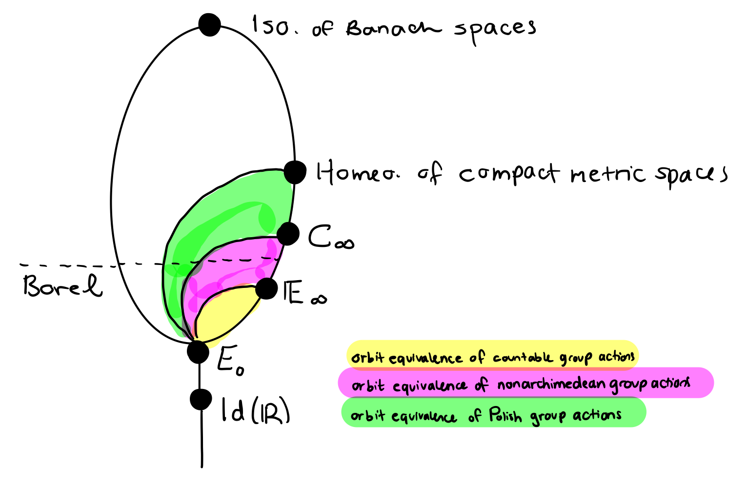
Figure 1. A partial illustration of analytic equivalence relations up to bireducibility. Below the dotted line are the Borel equivalence relations, where each equivalence class is a Borel set.

1.3. Results for proper homotopy equivalence of graphs

We first realize the set of locally finite graphs as a Polish space, in Section 2.2, which makes proper homotopy equivalence an analytic equivalence relation. Our main result is the following.

Theorem 1.1.

Proper homotopy equivalence on the space of locally finite graphs is bireducible with $C_{\infty}$. That is, the equivalence relation $\operatorname{\thicksim_{\text{PHE}}}$ is Borel complete.

We get the same complexity result when considering the subspaces of graphs of uniform or bounded degree. It should be noted that while being bireducible with $C_{\infty}$ is often reffered to as being “Borel complete,” the equivalence relations we are considering are not Borel equivalence relations. Our proof relies heavily on the result of Camerlo and Gao in [CG01] that the equivalence relation of homeomorphism on closed subsets of the Cantor set is bireducible with $C_{\infty}$.

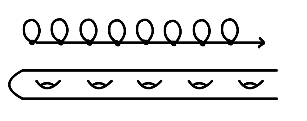
Figure 2. The Loch Ness Monster graph (top) and surface (bottom).

The graph formed by taking a ray and attaching infinitely many loops is often called the Loch Ness Monster graph (see fig. 2). This was after the corresponding surface, constructed from the plane by attaching handles along the positive real axis was named the Loch Ness Monster surface. Our second result shows that the equivalence classes of this graph is generic among infinite graphs.

Theorem 1.2.

The proper homotopy equivalence class of the Loch Ness Monster graph is a dense $G_{\delta}$ set in the space of locally finite, infinite graphs.

1.4. Results for homeomorphism of surfaces

In order to realize orientable surfaces as a Polish space, we endow them with a pants decomposition. Here a pants decomposition can mean a collection of simple closed curves on the surface up to isotopy so that the complementary components are $d$-holed spheres, for fixed, bounded, or finite $d$. See Section 2.3 for precise definitions of the spaces under consideration with examples.

Corollary 1.3.

The equivalence relation of homeomorphism on the space of surfaces with a pants decomposition is bireducible with $C_{\infty}$.

A version of the above corollary (where the result is the same, but the Polish space of surfaces is different) was proven by Bergfalk and Smythe in their upcoming preprint.

The analogous corollary to 1.2 for surfaces says that the homeomorphism class of the Loch Ness Monster surface is a dense $G_{\delta}$ set in the space of noncompact surfaces with a pants decomposition. We interpret this result as saying the following: If you randomly glue pairs of pants together to build a noncompact surface, that surface will almost surely be homeomorphic to a Loch Ness Monster surface. This holds true if you allow your building blocks to include annuli or pants with arbitrarily many legs.

1.5. Outline

In Section 2, we give some background information about the spaces we are working in and the tools we use. In Section 3 we prove 1.1 and 1.3 in the space of $3$-regular graphs. We show how to extend the proofs given in Section 3 to other spaces of graphs and surfaces in Section 4.

2. Background

2.1. Graphs

A graph $\Gamma$ is a triple consisting of two sets: the vertex set and the edge set, and an incidence relation between them associating to each edge two (not necessarily distinct) vertices. We call an edge which is incident to the same vertex twice a self-loop. This definition of a graph also allows for multiple edges, that is, edges which are incident to the same pair of vertices. Two distinct vertices are adjacent if they are incident to the same edge. An infinite graph is one where the vertex set or edge set is an infinite set.

The degree of a vertex, denoted $\deg(v)$, is the number of edges that are incident to it, counting multiplicity, so that a self-loop contributes degree two. We say a graph is locally finite if each vertex has finite degree. A graph is $k$-regular if every vertex in the graph has degree $k$. Note that locally-finite, infinite graphs necessarily have infinite vertex sets.

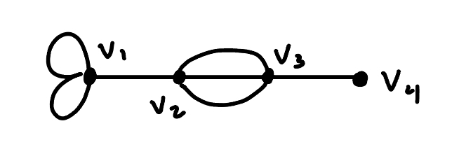
Figure 3. An example of a graph where $v_{1}$ has two self loops, and there are multiple edges between $v_{2}$ and $v_{3}$. The degree of $v_{1}$ is $5$, the degrees of $v_{2}$ and $v_{3}$ are $4$, and the degree of $v_{4}$ is $1$.

We realize a graph as a topological space by building the CW-complex with $0$-cells corresponding to the vertex set of $\Gamma$ and $1$-cells corresponding to the edge set of $\Gamma$. The $1$-cells are then glued to the $0$-cells by the incidence relation. The graph has a natural metric, called the path metric, which assigns each edge length one, so that adjacent vertices are distance one from each other. A graph is connected if it is connected as a CW complex; for the rest of the paper we will assume all graphs are connected. Note that connected, locally finite, infinite graphs necessarily have infinite but countable vertex and edge sets.

The fundamental group of a (connected) graph is always a free group, so we define the rank of a graph to be $\operatorname{rk}(\Gamma):=\operatorname{rk}(\pi_{1}(\Gamma))$. It is an exercise in algebraic topology to show that two graphs are homotopy equivalent exactly when they have the same rank. Because we will focus on infinite graphs, we will consider the equivalence relation of proper homotopy equivalence. Recall that a function between topological spaces is proper if the preimage of compact sets is compact. A proper homotopy equivalence is a continuous map $f:X\rightarrow Y$ which is proper with proper homotopy inverse $g:Y\rightarrow X$, so that both $f\circ g$ and $g\circ f$ are properly homotopic to identity maps. We study the equivalence relation of proper homotopy equivalence (PHE), and we will write $\Gamma\operatorname{\thicksim_{\text{PHE}}}\Delta$ if $\Gamma$ and $\Delta$ are PHE. The classification of locally finite, infinite graphs up to proper homotopy equivalence was done by Ayala, Dominguez, Márquez, and Quintero in [ADMQ90]. In order to understand the classification, we need to understand the end space of a graph.

Definition 2.1.

Let $\Gamma$ be a locally finite graph. The end space of ${\Gamma}$ is the following inverse limit with the inverse limit topology,

$$E(\Gamma):=\varprojlim_{K\subset\Gamma}\pi_{0}(\Gamma\setminus K),$$

where $K$ are compact subsets of ${\Gamma}$.

The end space will always be Hausdorff, totally disconnected, and compact, so a Stone space. Because graphs are Hausdorff, locally compact, and $\sigma$-compact, we can find a countable sequence of compact sets $K_{i}$ that obtain $E(\Gamma)$. Let $e\in E({\Gamma})$, and define the $i$th neighborhood of $e$, denoted $N_{i}(e)$, to be the component of $\Gamma\setminus K_{i}$ which contains $e$. We say that the end $e$ is accumulated by loops if $\operatorname{rk}(N_{i}(e))=\infty$ for all $i$. The set of ends of ${\Gamma}$ accumulated by loops is a closed subspace of $E(\Gamma)$, denoted by $E_{\ell}({\Gamma})$. Together $(E({\Gamma}),E_{\ell}({\Gamma}))$ are called the endspace pair of ${\Gamma}$. Endspace pairs $(E(\Gamma),E_{\ell}({\Gamma}))$ and $(E(\Delta),E_{\ell}(\Delta))$ are isomorphic if there is a homeomorphism $\phi:E(\Gamma)\rightarrow E(\Delta)$ with $\phi(E_{\ell}(\Gamma))=E_{\ell}(\Delta)$. We are now ready to state the proper homotopy equivalence classification theorem for graphs.

Theorem 2.2 ([ADMQ90, Theorem 2.7]).

Two locally finite graphs $\Gamma$ and $\Delta$ are proper homotopy equivalent exactly when $\operatorname{rk}(\Gamma)=\operatorname{rk}(\Delta)$ and $(E(\Gamma),E_{\ell}({\Gamma}))\simeq(E(\Delta),E_{\ell}(\Delta))$.

Figure 4 shows three graphs which are not proper homotopy equivalent to each other. The first graph is rank $3$ and has end space homeomorphic to $(\{\ast\},\emptyset)$, a singleton and the empty set. The second has infinite rank and end space homeomorphic to $(\{\frac{1}{n}\}\cup\{0\},\{0\})$, with the subspace topology from $\mathbb{R}$. The third graph has a Cantor set of ends, with a clopen subset (so itself homeomorphic to a Cantor set) of ends accumulated by loops.

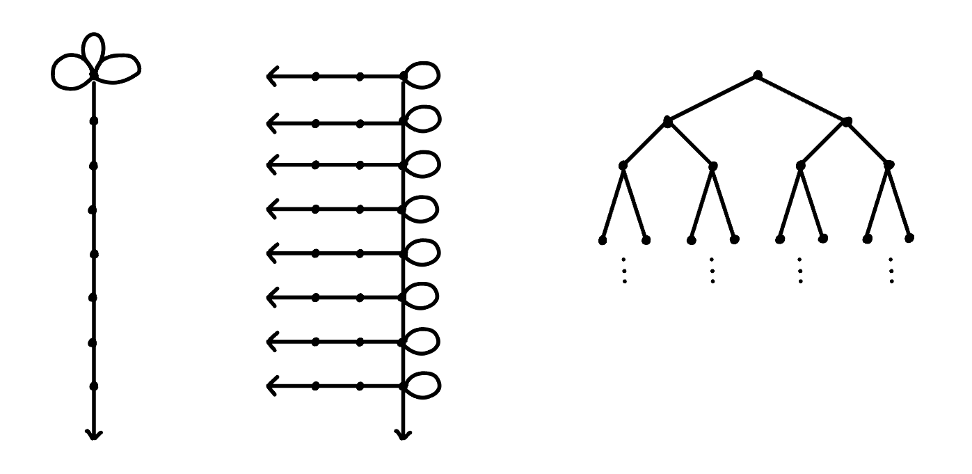
Figure 4. Examples of graphs with different end spaces. Each of these graphs have different PHE types.

2.2. Spaces of Graphs

We first define the set $\mathcal{G}_{k}$ to be the set of infinite, $k$-regular graphs with a basepoint, considered up to graph isomorphism fixing the basepoint. We topologize this set by comparing $r$-balls of the basepoint, denoted $B_{r}({\Gamma})$. We use $\cong$ to denote isomorphism fixing the base point. The following defines a metric on $\mathcal{G}_{k}$:

$$d(\Gamma_{1},\Gamma_{2})=\inf\left\{\frac{1}{2^{r}}\mid\;B_{r}(\Gamma_{1})\cong B_{r}(\Gamma_{2})\right\}.$$

Two graphs will be distance zero exactly when there is an isomorphism between them fixing the basepoint, so the metric topology is Haurdorff. The $\epsilon$-balls of the basepoints of any two graphs in $\mathcal{G}_{k}$ will be isomorphic for all ${\epsilon}<\frac{1}{2}$. Thus, the distance function is always finite valued and $\mathcal{G}_{k}$ is finite diameter. The sets

$$\mathcal{U}_{(\Gamma,r)}=\{\Delta\in\mathcal{G}_{k}\mid B_{r}({\Gamma})\cong B_{r}(\Delta)\},$$

form a clopen basis for the topology. The basis is clopen because the sets $\mathcal{U}_{({\Gamma},r)}$ and $\mathcal{U}_{({\Gamma},r+{\epsilon})}$ will agree when $[r,r+{\epsilon}]$ does not contain an integer or half-integer. Note that it is again very important that our graphs be connected, otherwise this topology will not be Hausdorff.

The space $\mathcal{G}_{1}$ is empty, and $\mathcal{G}_{2}$ is a singleton, corresponding to the graph which is homeomorphic to a line. The space $\mathcal{G}_{3}$ is our first infinite, non-discrete, Polish space, as are $\mathcal{G}_{k}$ for all $k\geq 4$. However, none of these spaces contain all PHE-types of infinite graphs. For example, there is only one $k$-regular tree for each $k$, and for $k\geq 3$ these all have end space homeomorphic to the Cantor set. So, we also consider the spaces $\mathcal{G}_{\leq k}$, which consists of infinite graphs where each vertex has degree less than or equal to $k$. We topologize the space in the exact same way as $\mathcal{G}_{k}$ above, allowing $r=0$, so that graphs with different degree basepoints are distance $1$ from each other. Each space $\mathcal{G}_{\leq k}$ for $k\geq 3$ contains every proper homotopy equivalence type of graph. To see this, start with the construction of standard models in Definition 2.5 of [AB21] and possibly apply proper homotopy equivalences as in fig. 5 to decrease the degree of any vertex. The final space we consider is $\mathcal{G}_{<\infty}$, which is the space of all locally finite, infinite graphs, again topologized in the same way. We will use the notation $\mathcal{G}_{\star}$ to denote any of the previously described spaces of graphs.

The degree of a vertex is not invariant under proper homotopy equivalence, so while we study the equivalence relation of PHE, note that the homotopies only necessarily live in $\mathcal{G}_{<\infty}$.

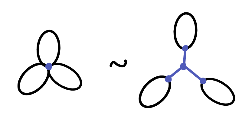
Figure 5. The graphs are proper homotopy equivalent, while the one on the left is $6$-regular, the one on the right is $3$-regular.

2.3. Surfaces

By surface we mean a second countable, Hausdorff, orientable, 2-manifold without boundary. A surface is of finite type if its fundamental group is finitely generated. Two finite-type surfaces are homeomorphic if they have the same number of genus and punctures. A surface is of infinite type if its fundamental group is not finitely generated. The classification of infinite-type surfaces predates, but is in direct analogy with, the classification of infinite graphs up to proper homotopy equivalence. It is due independently to Kerékjártó [Ker23] and Richards [Ric63].

Theorem 2.3.

Two surfaces $\Sigma$ and $\Sigma^{\prime}$ are homeomorphic exactly when $g(\Sigma)=g(\Sigma^{\prime})$ and
$(E(\Sigma),E_{g}(\Sigma))\simeq(E(\Sigma^{\prime}),E_{g}(\Sigma^{\prime}))$.

In this statement, $g(\Sigma)\in\mathbb{N}\cup\{0,\infty\}$ is the number of genus, $E(\Sigma)$ is the end space, and $E_{g}(\Sigma)$ is the subspace of ends accumulated by genus. The endspace of a surface can be defined mutatis mutandis with 2.1, replacing ${\Gamma}$ with $\Sigma$. To get the ends accumulated by genus, replace rank with genus in the definition of ends accumulated by loops.

2.3.1. Spaces of Surfaces

Next we want to realize sets of noncompact surfaces as Polish spaces; this includes infinite-type surfaces as well as finite-type surfaces with punctures. First, we define a pair of pants to be any orientable genus zero surface with at least one boundary component. If the pair of pants $P$ has $d+1$ boundary components we call them specifically a $d$-legged pair of pants, so that a $3$-holed sphere has two legs (the third boundary component being the waist). We allow $1$-legged pants, which are topologically annuli, and $0$-legged pants, which are topologically disks. A pants decomposition of a surface $S$ is a collection of subsurfaces $\mathcal{P}=\{P_{j}\}_{j\in I}$ which are each themselves pants, cover the surface $S$, and overlap exactly on their boundary components. Denote the boundary components of $P_{j}$ by $\{\partial_{1}P_{j},\dots,\partial_{d+1}P_{j}\}$. That is, $S$ can be constructed by gluing the pants together along their boundary components by orientation preserving homeomorphisms, and we can write

$$S=\left(\bigsqcup_{j\in I}P_{j}\right)/\left(\partial_{i}P_{j}\sim\partial_{k}P_{\ell}\right),$$

with each $\partial_{i}P_{j}$ appearing in the quotient exactly once. Note that our pants have boundary, so the only possible pants decomposition around a puncture is a sequence of annuli.

For any surface with a pants decomposition $(S,\mathcal{P})$ we associate a graph in the following way. For each pair of paints $P_{j}$, associate a vertex $v_{j}$. Whenever a boundary component of $P_{j}$ is glued to a boundary component of $P_{k}$, associate an edge from $(v_{j},v_{k})$, note that $j$ and $k$ may be equal. In this way, each $d$-legged pants corresponds to a vertex of degree $d+1$. If we consider surfaces with a basepoint interior to the pants decomposition, then we can associate a based graph. See fig. 6 for an example.

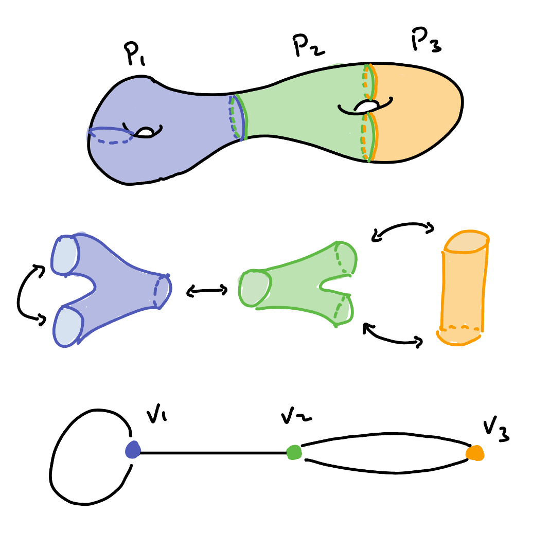
Figure 6. Constructing a graph from a surface with a pants decomposition.

For each space of graphs $\mathcal{G}_{\star}$ discussed in Section 2.2 we will define an analogous space of surfaces, $\mathcal{S}_{\star}$. The maps $\Phi_{\star}:\hat{\mathcal{S}_{\star}}\rightarrow\mathcal{G}_{\star}$ are surjective, so we can then endow $\hat{\mathcal{S}_{\star}}$ with the initial topology. Recall that the initial topology is the coarsest topology which makes $\Phi_{\star}$ continuous and has the sets

$$\mathcal{B}=\{\Phi^{-1}(\mathcal{U})\mid\mathcal{U}\text{ is open in }\mathcal{G}_{\star}\}$$

as a subbase. Note that this topology will not be Hausdorff. For example, the same surface with two pants decompositions in which pants curves are isotopic, but not equal, are indistinguishable by open sets in the topology. So, we quotient by the equivalence relation induced by $\Phi_{\star}$, that is $(S,\mathcal{P},b)\sim(S^{\prime},\mathcal{P}^{\prime},b^{\prime})$ if $\Phi_{\star}(S,\mathcal{P},b)=\Phi_{\star}(S^{\prime},\mathcal{P}^{\prime},b^{\prime})$. Call these quotient spaces (with the quotient topologies) $\mathcal{S}_{\star}$, and note that they are Hausdorff and homeomorphic to the corresponding space $\mathcal{G}_{\star}$. For detailed explanation, see for example Corollary 22.3 of Munkres’ Topology, [Mun00].

Points in $\mathcal{S}_{\star}$ can be thought of as surfaces, up to homeomorphism, with based pants decompositions, up to isotopy. A puncture on a surface will map to a ray in the associated graph. So, similar to the discussion of which graphs live in which spaces $\mathcal{G}_{\star}$, there are no surfaces with isolated punctures in $\mathcal{S}_{k}$ and all homeomorphism types of noncompact surfaces are realized in $\mathcal{S}_{\leq k}$ for $k\geq 3$.

2.4. Complexity of Borel equivalence relations

Our main result, 3.2, discusses the complexity of the proper homotopy equivalence relation on $\mathcal{G}_{n}$ for $n\geq 3$. To formalize what we mean by complexity, we need to introduce the notion of Borel reducibility of equivalence relations. For a more in depth introduction to this area, we refer the reader to [Tse22, Part 4].

By a Borel (resp., analytic) equivalence relation $E$ on a Polish space $X$, we mean that $E$ is a Borel (resp., analytic) subset of $X^{2}$ with respect to the product topology. For equivalence relations $E$ and $F$ on Polish spaces $X$ and $Y$, we say that $E$ is Borel reducible to $F$, and we write $E\leq_{B}F$, if there is a Borel function $\phi:X\to Y$ so that $(x,y)\in E$ if and only if $(\phi(x),\phi(y))\in F$. In other words, to check whether two points are $E$-equivalent, we can pass the points to $Y$ via our Borel function and check whether the images are $F$-equivalent. In this case, we say that $\phi$ is a Borel reduction from $E$ to $F$. We say that $E$ is Borel bireducible with $F$ (or that $E$ and $F$ are Borel equivalent) if $E\leq_{B}F$ and $F\leq_{B}E$.

An equivalence relation $E$ is called concretely classifiable (or smooth) if there is a Borel reduction from $E$ to the equality relation on some Polish space $Y$. For example, similarity of $n\times n$ matrices is smooth since similarity is determined by computing the Jordan canonical form. However, many notable equivalence relations are not smooth. We say that $E$ is classifiable by countable structures if for some countable language $\mathcal{L}$, there is a Borel reduction from $E$ to the isomorphism relation of the space of $\mathcal{L}$-structures with universe $\mathbb{N}$.

By [BK96], there is an orbit equivalence relation, denoted $C_{\infty}$, induced by a Borel action of $S_{\infty}$ (the Polish group of all permutations of $\mathbb{N}$) that is “complete” in the sense that any orbit equivalence relation induced by a Borel action of a closed subgroup of $S_{\infty}$ is Borel reducible to $C_{\infty}$. In the literature, analytic equivalence relations which are bireducible with $C_{\infty}$ are often referred to as Borel complete. We will see in 3.2 that the proper homotopy equivalence relation on each of the spaces $\mathcal{G}_{\star}$ is Borel complete.

An important class of analytic equivalence relations that are reducible to $C_{\infty}$ are those that are classifiable by countable structures: if $\mathcal{L}$ is a countable language, then the isomorphism relation of the space of $\mathcal{L}$-structures can be viewed as an $S_{\infty}$ orbit equivalence relation (see, e.g. [Kec95, 16.C]).

3. Proofs of main results for 3-regular graphs

We begin by showing that every closed subset of the Cantor set can be found as the endspace of a graph in $\mathcal{G}_{3}$. This allows us to define a Borel reduction from the homeomorphism relation on closed subsets of the Cantor set to the PHE relation.

Lemma 3.1.

For any closed subset $C$ of the Cantor space, $C$ is realized as the end space accumulated by loops of some $\Gamma_{C}\in\mathcal{G}_{3}$. Moreover, $\Gamma_{C}$ can be taken to have all of its ends accumulated by loops.

Proof.

We use the standard identification of $2^{\mathbb{N}}$ with the Cantor set and with ends of a rooted binary tree. Let $C\subseteq{2^{\mathbb{N}}}$ be closed and not a singleton. Let ${\Gamma}_{C}^{*}$ be the subgraph of the rooted binary tree with endspace $C$ and no leaves. Note that every vertex in $\Gamma_{C}^{*}$ has valence $2$ or $3$. Let $\Gamma_{C}$ be the graph obtained by subdividing each edge of ${\Gamma}_{C}^{*}$ and then adding “lollipops” to each vertex of degree two, as illustrated in fig. 7. This modification doesn’t add or collapse any ends, so the resulting graph $\Gamma_{C}$ has $E({\Gamma_{C}})=E_{\ell}({\Gamma_{C}})=C$, and is of infinite rank.

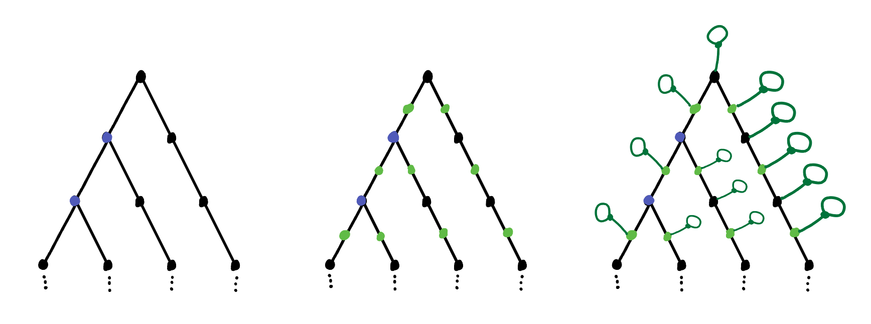
Figure 7. Modifying a graph $\Gamma_{C}^{*}$ (left) so that it is in $\mathcal{G}_{3}$ by subdividing edges (middle) and then adding lollipops to degree $2$ vertices (right).

If $C$ is a singleton, then an example of a graph ${\Gamma}_{C}$ in $\mathcal{G}_{3}$ is given in fig. 8.

∎

We are now ready to prove our main theorem for the space $\mathcal{G}_{3}$.

Theorem 3.2.

Proper homotopy equivalence on $\mathcal{G}_{3}$ is bireducible with $C_{\infty}$. That is, $\operatorname{\thicksim_{\text{PHE}}}$ is Borel complete.

Proof.

We start by showing that $C_{\infty}\leq_{B}\;\operatorname{\thicksim_{\text{PHE}}}$. By [CG01], it suffices to demonstrate a Borel reduction from the homeomorphism relation for closed subsets of the Cantor space to $\operatorname{\thicksim_{\text{PHE}}}$ on $\mathcal{G}_{3}$. This follows from 3.1 and the observation that the assignment $C\mapsto\Gamma_{C}$ in the proof of 3.1 is Borel. Indeed, because each nonempty basic open subset of $\mathcal{G}_{3}$ is determined by finitely many conditions on the graph; hence, the preimage of the set is Borel in $\mathcal{K}(2^{\mathbb{N}})$. Hence, the map $\phi:\mathcal{K}(2^{\mathbb{N}})\to\mathcal{G}_{3}$ defined by $C\mapsto\Gamma_{C}$ is a Borel reduction of homeomorphisms of closed subsets of $2^{\mathbb{N}}$ to $\operatorname{\thicksim_{\text{PHE}}}$, as desired.

Next we show the other direction, that $\operatorname{\thicksim_{\text{PHE}}}\;\leq_{B}\;C_{\infty}$; we give the intuition before the formal argument.

Intuitively: 2.2 tells us that two graphs are proper homotopy equivalent when they have the same rank and simultaneously homeomorphic endspace pairs. Each part of the endspace pair is homeomorphic to a closed subset of $2^{\mathbb{N}}$, the Cantor set. By [CG01], the homeomorphism relation on closed subsets of $2^{\mathbb{N}}$ is bireducible with isomorphism of countable structures. Since homeomorphism is the most complicated aspect of $\operatorname{\thicksim_{\text{PHE}}}$, we have the desired Borel reduction.

Formally: We use a similar argument to the one in [CG01]. Let $\mathcal{K}(2^{\mathbb{N}})$ be the space of closed subsets of the Cantor space, equipped with the Vietoris topology. Let $\mathcal{L}$ be the language of Boolean algebras $\{\vee,\wedge,-,0,1\}$, along with an extra constant symbol $n$, unary relation symbols $K$ and $L$, and unary function symbol $f$. Let $\mathcal{T}$ be the axioms of Boolean algebras along with a sentence asserting that $K$ and $L$ are disjoint, and that $f$ is a surjection from $K$ to $L$. Let $\mathcal{M}$ be the space of models of $\mathcal{T}$ with universe $\mathbb{N}$.

To each $\Gamma\in\mathcal{G}_{k}$ with rank $\operatorname{rk}(\Gamma)\in\mathbb{N}\cup\{\mathbb{N}\}$, end space $E(\Gamma)$, and end space accumulated by loops $E_{\ell}(\Gamma)$, we associate the countable structure $\mathcal{B}_{\Gamma}\in\mathcal{M}$:

$$(n_{\Gamma},K_{\Gamma},L_{\Gamma},f_{\Gamma},\vee,\wedge,-,0,1)$$

where:

• $n_{\Gamma}=\text{rk}_{\Gamma}+1$ if $\text{rk}_{\Gamma}\in\mathbb{N}$ or $n_{\Gamma}=0$ if $\text{rk}_{\Gamma}=\mathbb{N}$,

• $K_{\Gamma}$ is the Boolean algebra of clopen subsets of $E(\Gamma)$,

• $L_{\Gamma}$ is the Boolean algebra of clopen subsets of $E_{\ell}(\Gamma)$,

• $f_{\Gamma}$ is the (surjective) map $f_{\Gamma}:K_{\Gamma}\to L_{\Gamma}$ defined by $Y\mapsto Y\cap E_{\ell}(\Gamma)$,

• and $\vee,\wedge,-,0,1$ are the usual Boolean operations.

By the usual proof of Stone duality, $\Gamma_{1}\operatorname{\thicksim_{\text{PHE}}}\Gamma_{2}$ if and only if $\mathcal{B}_{\Gamma_{1}}\cong\mathcal{B}_{\Gamma_{2}}$. To see that the assignment $\Gamma\mapsto\mathcal{B}_{\Gamma}$ is Borel, we first note that the assignments $\Gamma\mapsto n_{\Gamma}\in\mathbb{N}$, $\Gamma\mapsto E(\Gamma)\in\mathcal{K}(2^{\mathbb{N}})$, and $\Gamma\mapsto E_{\ell}(\Gamma)\in\mathcal{K}(2^{\mathbb{N}})$ are Borel. Note also that the Boolean operations are Borel over the space $\mathcal{K}(2^{\mathbb{N}})$.

It remains to verify that the assignments $\Gamma\mapsto K_{\Gamma}$ and $\Gamma\mapsto L_{\Gamma}$ are Borel. As in [CG01], we from a canonical enumeration of the clopen subsets of $2^{\mathbb{N}}$, denoted $\{\mathcal{O}^{\prime}_{i}\}_{i\in\mathbb{N}}$. To disjointify $K_{\Gamma}$ and $L_{\Gamma}$, we modify the enumeration to $\{\mathcal{O}_{i}\}_{i\in\mathbb{N}}$, where $\mathcal{O}_{2i}=\mathcal{O}_{2i+1}=\mathcal{O}^{\prime}_{i}$.

We first enumerate the clopen subsets of $E(\Gamma)$ and $E_{\ell}(\Gamma)$ respectively as $\{\mathcal{O}_{2i}\cap E(\Gamma)\}_{i\in\mathbb{N}}$ and $\{\mathcal{O}_{2i+1}\cap E_{\ell}(\Gamma)\}_{i\in\mathbb{N}}$, possibly with repetitions. Now let $\rho$ be the enumeration of the sequence $\{\mathcal{O}_{2i}\cap E(\Gamma)\}_{i\in\mathbb{N}}$ without repetitions (but preserving the order), and let $\rho_{\ell}$ be the enumeration of the sequence $\{\mathcal{O}_{2i+1}\cap E_{\ell}(\Gamma)\}_{i\in\mathbb{N}}$ without repetitions (but preserving the order). Then $\rho$ and $\rho_{\ell}$ are Borel functions that uniquely describe $K_{\Gamma}$ and $L_{\Gamma}$. ∎

We close this section by showing that $\operatorname{\thicksim_{\text{PHE}}}$ on $\mathcal{G}_{3}$ has a dense $G_{\delta}$ equivalence class, the class of one-ended graphs with infinite rank. This is the Loch Ness monster equivalence class, and the graphs in fig. 8 are examples.

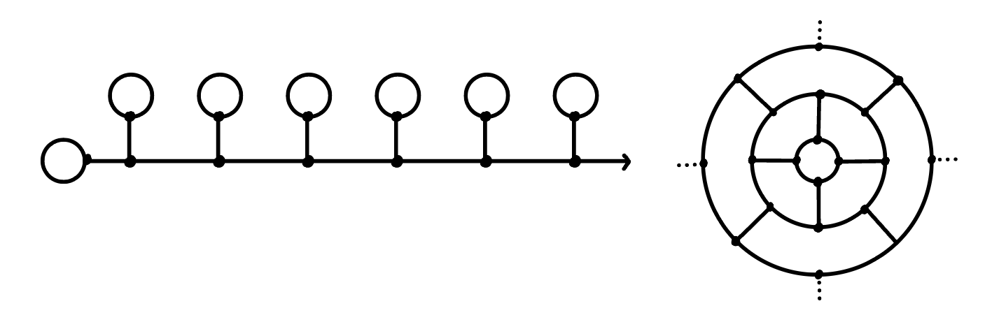
Figure 8. Two representatives of the generic proper homotopy equivalence class of graphs in $\mathcal{G}_{3}$.

It is perhaps unsurprising that the generic graph is of infinite rank, since avoiding loops in the construction of a graph is quite restrictive. The key to showing that both finite rank and one-endedness are generic will be that rank and connectedness can be checked for inside balls of finite radius.

Proposition 3.3.

The equivalence class of one-ended graphs with infinite rank is dense $G_{\delta}$ in $\mathcal{G}_{3}$.

Proof.

First, we claim that the set of graphs in $\mathcal{G}_{3}$ with infinite rank is a dense $G_{\delta}$ set. Let $U_{n}$ be the graphs in $\mathcal{G}_{3}$ with rank at least $n$. Each set $U_{n}$ is open because for any $\Gamma\in U_{n}$, there is an $r\in\mathbb{N}$ such that $B_{r}(\Gamma)$ already has rank $n$. Then $\mathcal{U}_{(\Gamma,r)}\subseteq U_{n}$. To see that $U_{n}$ is dense, we show that for any $\Gamma\in\mathcal{G}_{3}$ and $r\in\mathbb{N}$, we can find $\Delta_{U}$ with rank at least $n$ and $B_{r}(\Delta_{U})\cong B_{r}({\Gamma})$. Such a graph $\Delta_{U}$ can be constructed from ${\Gamma}$ by subdividing $n$ edges of ${\Gamma}$ outside of $B_{r}({\Gamma})$ and attaching lollipop graphs to the new vertices. We finish the claim by observing that $\bigcap U_{n}$ is exactly the set of graphs of infinite rank.

Now we verify that the generic $\Gamma$ is one-ended. Let $V_{n}$ be the set of $\Gamma\in\mathcal{G}_{3}$ such that each pair of vertices in the sphere of radius $n$ of $\Gamma$ is path-connected outside of $B_{n}(\Gamma)$. If a graph $\Gamma$ is one ended, then eventually ${\Gamma}\setminus B_{r}({\Gamma})$ has one connected component, so the set of one-ended graphs is $\bigcup_{i\in\mathbb{N}}\bigcap_{n\geq i}V_{n}$. Each $V_{n}$ is open because for ${\Gamma}\in V_{n}$ there is a finite path between any two vertices on the $n$-sphere. All these paths live inside some $B_{r}({\Gamma})$, for $r\geq n$, and so $\mathcal{U}_{({\Gamma},r)}\subset V_{n}$. To see that $V_{n}$ is dense, we construct a graph $\Delta_{V}$ from any $\Gamma\in\mathcal{G}_{3}$ so that $\Delta_{V}\in V_{n}$ with $B_{r}(\Delta_{V})\cong B_{r}(\Gamma)$. For each pair of connected components of ${\Gamma}\setminus B_{r}({\Gamma})$ subdivide an edge in each component and add an edge between the new vertices, see fig. 9. Because there are finitely many vertices on the $n$-sphere of ${\Gamma}$, there are finitely many connected components, and the modifications can be done successively in any order to construct the desired graph $\Delta_{V}$.

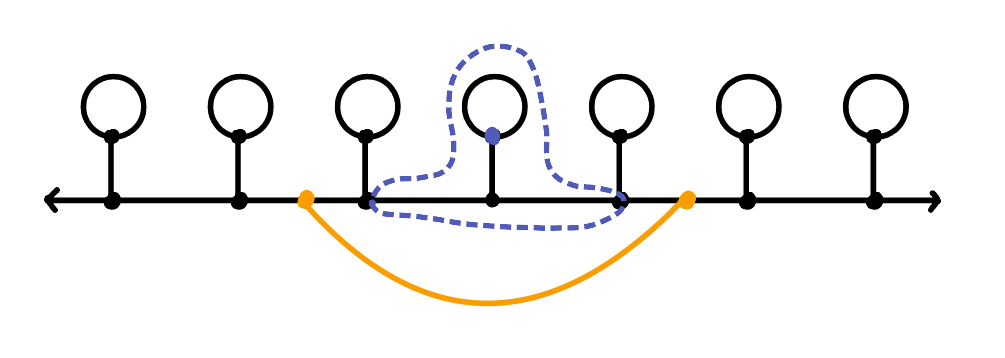
Figure 9. For the black graph ${\Gamma}$, the ball of radius $2$ is drawn in blue. To find a one-ended graph in $\mathcal{U}_{({\Gamma},2)}$ we add the orange edge.

Because having infinite rank and one end are each generic properties and determine a unique PHE class, we see that the equivalence class of the Loch Ness monster graph is dense $G_{\delta}$. ∎

4. Extending the results to other spaces

We begin with a version of 3.1 for larger values of $k$.

Lemma 4.1.

For every $k>3$ and any closed subset $C$ of the Cantor space, $C$ is realized as the end space accumulated by loops of some $\Gamma_{C}^{k}\in\mathcal{G}_{k}$. Moreover, $\Gamma_{C}^{k}$ can be taken to have all of its ends accumulated by loops.

Proof.

We begin as in 3.1 with $C\subset 2^{\mathbb{N}}$, not a singleton, and the graph ${\Gamma}_{C}^{*}$. For each value of $k$ we describe how to modify ${\Gamma}_{C}^{*}$ to get a graph in $\mathcal{G}_{k}$ with $E({\Gamma}_{C}^{k})=E_{\ell}({\Gamma}_{C}^{k})=C$.

For $k$ odd, perform the following modifications to ${\Gamma}_{C}$:

• for each degree $3$ vertex add $\frac{k-3}{2}$ self-loops,

• for each degree $2$ vertex add a new vertex, connect them by $k-2$ edges, and add a self-loop to the new vertex.

This process adds loops to each vertex, so ultimately every end is accumulated by loops. See fig. 10 for an example where $k=7$.

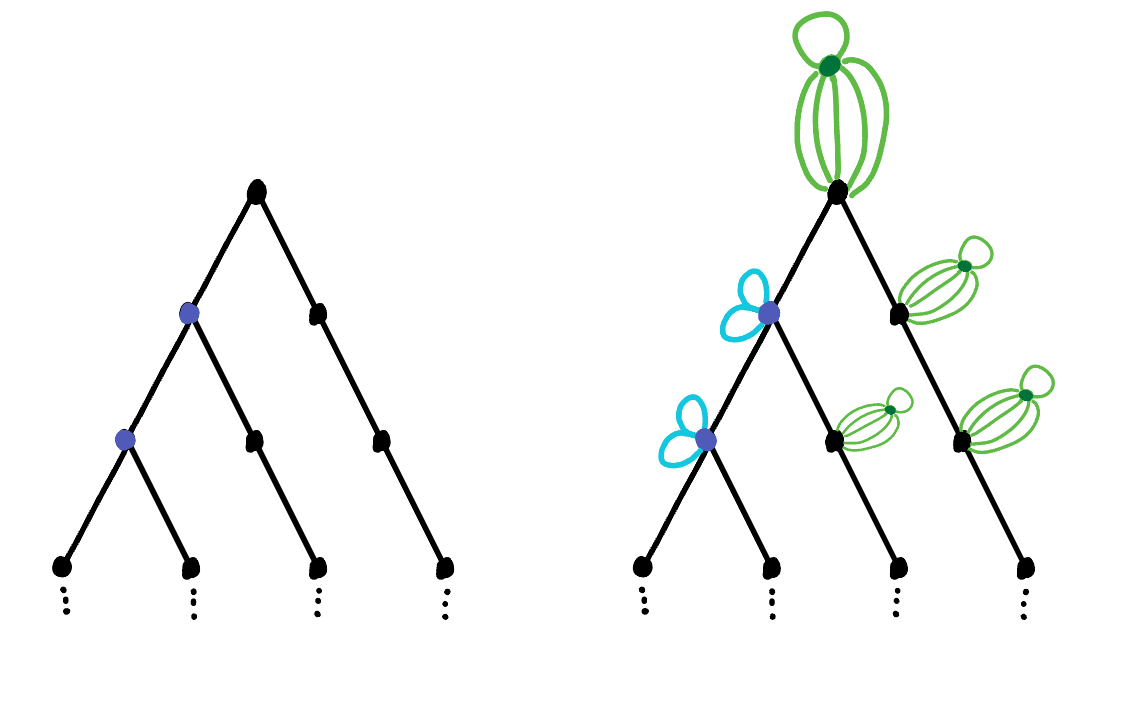
Figure 10. Modifying the graph ${\Gamma}_{C}$ so that it is in $\mathcal{G}_{7}$.

For $k$ even, $k\neq 4$, we first double every edge of $\Gamma_{C}$ so that every vertex has degree $4$ or $6$. Then

• for each degree $4$ vertex add $\frac{k-4}{2}$ self-loops,

• for each degree $6$ vertex add $\frac{k-6}{2}$ self-loops.

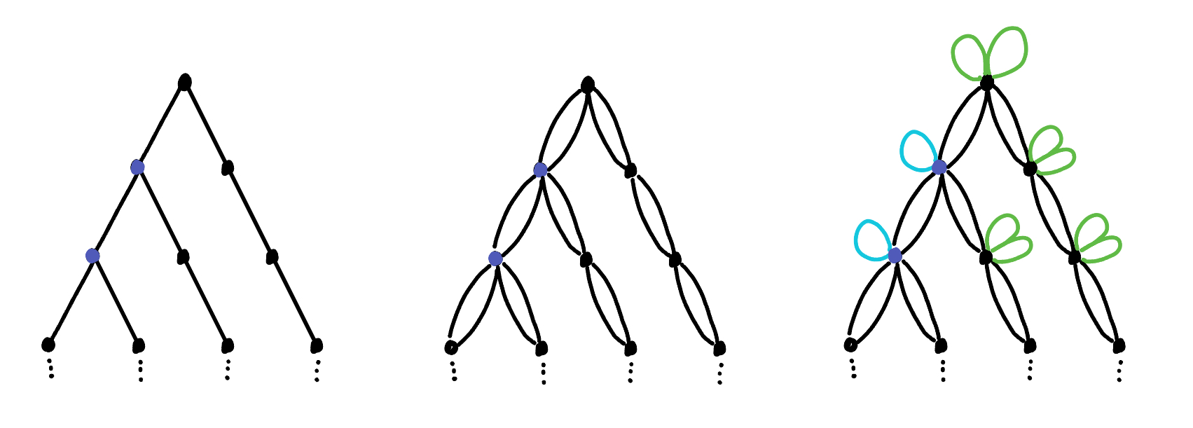
Figure 11. Modifying the graph ${\Gamma}^{*}_{C}$ so that it is in $\mathcal{G}_{8}$, first by doubling edges, then adding self-loops.

Finally, the case where $k=4$ requires a bit more subtlety. First double every edge of ${\Gamma}_{C}$ and then perform a local PHE at every degree $6$ vertex to split it into two degree $4$ vertices, as in fig. 12. Because these are disjoint, compactly supported, homotopy equivalences, they do not change the PHE type of the graph, and in particular do not change the end space. Note that after doubling edges, every end of the graph was accumulated by loops.

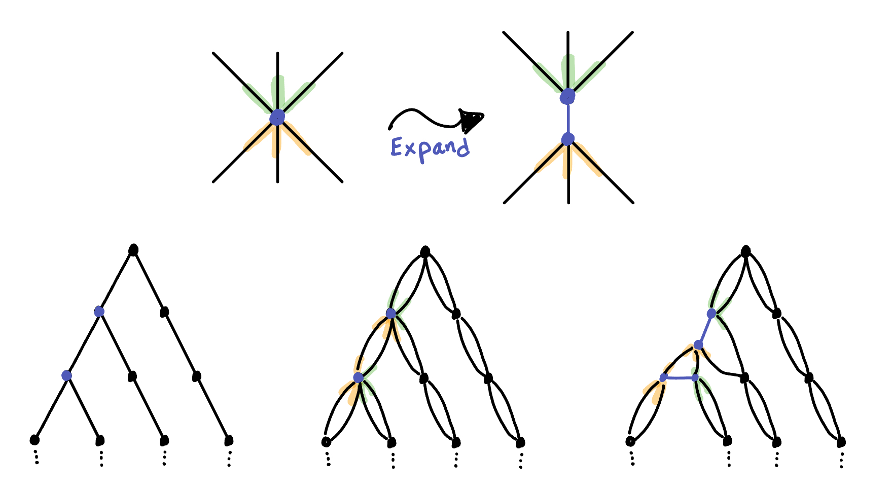
Figure 12. A local PHE is done at each degree $6$ vertex to split it into two degree $4$ vertices. The choice of grouping of the $6$ edges into groups of $3$ does not affect the PHE type of the graph.

When $C$ is a singleton, we take ${\Gamma}_{C}^{*}$ to be a ray graph, so it has one vertex of degree $1$, call it $v$. To construct ${\Gamma}_{C}^{k}$, follow the instructions above with the following modifications for the degree one vertex.

• For $k$ odd, add $\frac{k-1}{2}$ self-loops to $v$.

• For $k$ even, after doubling edges $v$ will have degree $2$, so add $\frac{k-2}{2}$ self-loops.

∎

The only place the $3$-regularity was used in the proof of 3.2 was 3.1. So, with 4.1 in hand, we have the complexity result for each space $\mathcal{G}_{k}$. Because $\mathcal{G}_{k}\subset\mathcal{G}_{\leq k}\subset\mathcal{G}_{\infty}$, we get the complexity result for each space $\mathcal{G}_{\star}$.

Corollary 4.2 (Intro 1.1 expanded).

Proper homotopy equivalence on $\mathcal{G}_{k}$, $\mathcal{G}_{\leq k}$, or $\mathcal{G}_{<\infty}$ is bireducible with $C_{\infty}$. That is, the equivalence relation $\operatorname{\thicksim_{\text{PHE}}}$ is Borel complete.

Next we show that the Loch Ness monster graph is still generic in the other spaces of infinite graphs.

Proposition 4.3 (Intro 1.2 expanded).

The equivalence class of one-ended graphs with infinite rank is dense $G_{\delta}$ in $\mathcal{G}_{k}$, $\mathcal{G}_{\leq k}$, and $\mathcal{G}_{<\infty}$.

Proof.

Following the proof of 3.3, we just need to modify the constructions of $\Delta_{U}$ and $\Delta_{V}$ to show that the corresponding sets $U_{n}$ and $V_{n}$ are dense in each $\mathcal{G}_{k}$. For each step we start with any graph ${\Gamma}\in\mathcal{G}_{k}$ and construct $k$-regular graphs, called $\Delta_{U}^{k}$ and $\Delta_{V}^{k}$, with the desired property.

1. To construct $\Delta_{U}^{k}$: subdivide $n$ edges of ${\Gamma}$ outside of $B_{r}({\Gamma})$ and attach the following graphs to the new vertices.

   • For even $k$, attach $k-2$ self loops.

   • For odd $k$, attach the barrel cactus graphs from 4.1 and fig. 10. That is, for each vertex from the subdivision, add another vertex, connect them by $k-2$ edges, and add a self-loop to the new vertex.

2. To construct $\Delta_{V}^{k}$: For each pair of connected components of ${\Gamma}\setminus B_{r}({\Gamma})$ subdivide an edge in each and add $k-2$ edges between the new vertices.

Because a $k$-regular graph is also in $\mathcal{G}_{\leq k}$, and $\mathcal{G}_{<\infty}$, this concludes the proof for all spaces. ∎

When we defined the spaces $\mathcal{G}_{\star}$ we required that the graphs be infinite. We can drop this requirement and define analogous spaces with the same topology, call them $\mathcal{G}^{\prime}_{\star}$. These spaces will look the same as before but with the addition of the countably many finite graphs, which are all isolated points in the topology. The complexity of $\operatorname{\thicksim_{\text{PHE}}}$ does not change, since $\mathcal{G}_{\leq k}\subseteq\mathcal{G}^{\prime}_{\leq k}$ and the restriction of $\operatorname{\thicksim_{\text{PHE}}}$ to the set of finite graphs is smooth since rank is a Borel function from the space of finite graphs to $\mathbb{N}$. However, there is no longer a dense $G_{\delta}$ equivalence class, since each finite graph is an isolated point in the topology. When we construct surfaces from the finite graphs we get compact surfaces with a pants decomposition in the analogously defined spaces $\mathcal{S}^{\prime}_{\star}$. Because the homeomorphisms between $\mathcal{G}^{\prime}_{\star}$ and $\mathcal{S}^{\prime}_{\star}$ respect the equivalence classes of finite graphs and compact surfaces, which are determined only by rank and genus, we get all the analogous results for $\mathcal{S}_{\star}$. The conclusions of this discussion are summarized in the table below.

Space $(k\geq 3)$	Complexity class	Dense $G_{\delta}$ equivalence class?
$\mathcal{G}_{k}$, $\mathcal{G}_{\leq k}$, $\mathcal{G}_{\leq\infty}$	$C_{\infty}$	Yes: Loch Ness Monster Graph
$\mathcal{G}^{\prime}_{k}$, $\mathcal{G}^{\prime}_{\leq k}$, $\mathcal{G}^{\prime}_{\leq\infty}$	$C_{\infty}$	No
$\mathcal{S}_{k}$, $\mathcal{S}_{\leq k}$, $\mathcal{S}_{\leq\infty}$	$C_{\infty}$	Yes: Loch Ness Monster Surface
$\mathcal{S}^{\prime}_{k}$, $\mathcal{S}^{\prime}_{\leq k}$, $\mathcal{S}^{\prime}_{\leq\infty}$	$C_{\infty}$	No

Table 1. Summary of results.

References

- [AB21] Yael Algom-Kfir and Mladen Bestvina, Groups of proper homotopy equivalences of graphs and Nielsen realization, arXiv preprint arXiv:2109.06908 (2021), To appear in Contemp. Math.
- [ADMQ90] R. Ayala, E. Dominguez, A. Márquez, and A. Quintero, Proper homotopy classification of graphs, Bull. London Math. Soc. 22 (1990), no. 5, 417–421. MR 1082009
- [BK96] H. Becker and A. S. Kechris, The descriptive set theory of Polish group actions, London Mathematical Society Lecture Note Series, vol. 232, Cambridge University Press, Cambridge, 1996. MR 1425877
- [CG01] Riccardo Camerlo and Su Gao, The completeness of the isomorphism relation for countable Boolean algebras, Trans. Amer. Math. Soc. 353 (2001), no. 2, 491–518. MR 1804507
- [DJK94] R. Dougherty, S. Jackson, and A. S. Kechris, The structure of hyperfinite Borel equivalence relations, Trans. Amer. Math. Soc. 341 (1994), no. 1, 193–225. MR 1149121
- [FLR09] Valentin Ferenczi, Alain Louveau, and Christian Rosendal, The complexity of classifying separable Banach spaces up to isomorphism, J. Lond. Math. Soc. (2) 79 (2009), no. 2, 323–345. MR 2496517
- [Kec95] A. S. Kechris, Classical descriptive set theory, Grad. Texts in Math., vol. 156, Springer, 1995.
- [Ker23] B. v. Kerékjártó, Vorlesungen über topologie. i, Spring, Berlin, 1923.
- [Mun00] J.R. Munkres, Topology, Featured Titles for Topology, Prentice Hall, Incorporated, 2000.
- [Ric63] Ian Richards, On the classification of noncompact surfaces, Trans. Amer. Math. Soc. 106 (1963), 259–269. MR 143186
- [Tse22] A. Tserunyan, Introduction to descriptive set theory, Preprint (2022), https://www.math.mcgill.ca/atserunyan/Teaching_notes/dst_lectures.pdf.
- [Zie16] Joseph Zielinski, The complexity of the homeomorphism relation between compact metric spaces, Adv. Math. 291 (2016), 635–645. MR 3459026