GSPR: Multimodal Place Recognition Using 3D Gaussian Splatting for Autonomous Driving

Abstract

Place recognition is a crucial module to ensure autonomous vehicles obtain usable localization information in GPS-denied environments. In recent years, multimodal place recognition methods have gained increasing attention due to their ability to overcome the weaknesses of unimodal sensor systems by leveraging complementary information from different modalities. However, challenges arise from the necessity of harmonizing data across modalities and exploiting the spatio-temporal correlations between them sufficiently. In this paper, we propose a 3D Gaussian Splatting-based multimodal place recognition neural network dubbed GSPR. It explicitly combines multi-view RGB images and LiDAR point clouds into a spatio-temporally unified scene representation with the proposed Multimodal Gaussian Splatting. A network composed of 3D graph convolution and transformer is designed to extract high-level spatio-temporal features and global descriptors from the Gaussian scenes for place recognition. We evaluate our method on the nuScenes dataset, and the experimental results demonstrate that our method can effectively leverage complementary strengths of both multi-view cameras and LiDAR, achieving SOTA place recognition performance while maintaining solid generalization ability. Our open-source code is available at https://github.com/QiZS-BIT/GSPR.

I Introduction

Given an observation from sensors at the current moment (query), place recognition needs to determine which location in the global map (database) the observation corresponds to. Place recognition is an important module in most navigation systems, capable of correcting accumulated drift in SLAM algorithms and often serving as the first step in global localization. In autonomous driving systems, cameras are commonly used for vision-based place recognition (VPR), providing rich semantics and texture information [1, 2, 3]. However, vision features extracted from camera images exhibit lower stability and result in suboptimal recognition accuracy when facing variations in lighting, seasons, and weather in large-scale outdoor environments. In contrast, LiDAR sensors show high stability against these factors, leading to more robust LiDAR-based place recognition (LPR) in large-scale outdoor scenes [4, 5, 6]. However, the recognition performance of LPR is still limited by the natural sparsity of LiDAR point clouds, and the lack of texture and semantic information.

In recent years, multimodal place recognition (MPR) methods such as MinkLoc++ [7] and LCPR [8] have demonstrated the potential advantages of fusing data from complementary camera and LiDAR modalities, attracting more research interests. However, most MPR methods independently extract features from primitive representations of scenes, i.e., raw images and point clouds, and implement unexplainable feature-level fusion. This results in insufficient exploitation of the spatio-temporal correlations between different modalities. Therefore, how to effectively fuse multimodal sensor data into a unified scene representation and fully extract multimodal spatio-temporal correlations remains a topic worthy of further research. Recently, 3D Gaussian Splatting (3D-GS) [9] is proposed to construct an explicit scene representation using 3D Gaussians, ensuring fast rendering of novel view while effectively capturing accurate geometry information. By aggregating temporally continuous observations from multiple views, 3D-GS constructs spatial structural representations comprehensively, providing the possibility for spatio-temporal fusion of multimodal place recognition.

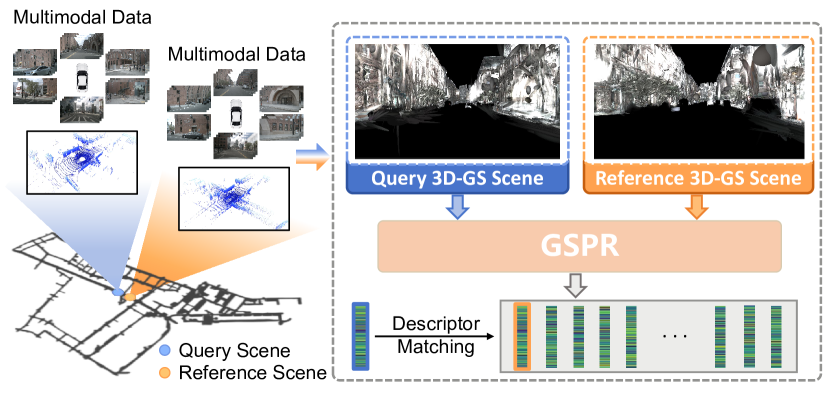
Figure 1: Effectively integrating different modalities is crucial for leveraging multimodal data. GSPR harmonizes multi-view RGB images and LiDAR point clouds into a unified scene representation based on Multimodal Gaussian Splatting. 3D graph convolution and transformer are utilized to extract both local and global spatio-temporal information embedded in the scene. This approach enables the generation of discriminative descriptors for place recognition.

In this paper, we propose a 3D Gaussian Splatting-based multimodal place recognition method namely GSPR, as shown in Fig. 1. We first design a Multimodal Gaussian Splatting (MGS) method to represent autonomous driving scenarios. We utilize LiDAR point clouds as a prior for the initialization of Gaussians, which helps to address the failures of structure-from-motion (SfM) in such environments. In addition, a mixed masking mechanism is employed to remove unstable features less valuable for place recognition. By doing so, we fuse multimodal data into a spatio-temporally unified Gaussian scene representation. We then downsample the unordered Gaussians within each scene into a set of voxels through voxel partitioning, and develop a network based on 3D graph convolution and transformer to extract high-level spatio-temporal features for generating discriminative descriptors for place recognition. Through the proposed Multimodal Gaussian Splatting, we fuse multimodal data into a unified explicit scene representation, providing a foundation for spatio-temporal fusion of multimodal place recognition.

In summary, our main contributions are as follows:

• We propose Multimodal Gaussian Splatting method to harmonize multi-view camera and LiDAR data into a spatio-temporally unified explicit scene representation.

• We propose GSPR, a novel MPR network equipped with 3D graph convolution and transformer to aggregate high-level local and global spatio-temporal information inherent in the MGS scene representation.

• Extensive experimental results demonstrate that our method outperforms the state-of-the-art unimodal and multimodal methods on place recognition performance while showing a solid generalization ability on unseen driving scenarios.

II Related Work

II-A Scene Representation in Place Recognition

Place recognition is a classic topic in the fields of robotics and computer vision, and there have been various types of traditional methods based on handcrafted descriptors [10, 1, 11]. With the rapid development of deep learning, an increasing number of learning-based approaches [2, 12, 4, 5, 6] have been proposed and overall present better recognition performance than traditional counterparts.

In place recognition tasks, autonomous vehicles perceive the environment through cameras or LiDAR sensors and attempt to build a reasonable scene representation corresponding to the place where the vehicle is situated. The input form of place recognition methods is closely related to the type of sensors. Most vision-based place recognition methods [2, 12, 13, 14] treat RGB images as trivial scene representations. NetVLAD [2] aggregates features from RGB images into global descriptors. Building on this, SPE-NetVLAD [12] and Patch-NetVLAD [3] introduces a focus on local image features, enhancing the place recognition performance in complex environments. R2Former [13] directly inputs RGB images into transformers for image retrieval and re-ranking. SALAD [14] aggregates image features using optimal transport algorithm, producing discriminative descriptors. LiDAR or Radar-based place recognition [15, 16, 17, 18, 8], on the other hand, uses sparse point cloud representations from range detection to depict driving scenes. For instance, PointNetVLAD [4] uses submaps obtained by stacking LiDAR point clouds as the scene representation, Autoplace [16] uses BEV views constructed from multi-view radars to capture structural information of the scene, OverlapNet [19] obtains dense depth information by projecting unordered LiDAR point clouds into range images, and CVTNet [18] combines multi-layer BEVs and range images to alleviate the information loss of 3D point cloud projection. However, these primitive scene representations typically fail to adequately reflect the spatio-temporal correlation within the scene. Our method, utilizing 3D-GS, generates unified explicit scene representations, which encompass richer and more harmonized spatio-temporal information compared to primitive representations.

II-B Multimodal Place Recognition

Recently, multimodal place recognition has aroused great interest due to its ability to leverage the complementary advantages of multiple sensors. PIC-Net proposed by Lu et al. [20] uses global channel attention to fuse descriptors from point clouds and images. MinkLoc++ [7] concatenates point cloud descriptors from sparse convolutions with image descriptors from pre-trained ResNet Blocks. AdaFusion proposed by Lai et al. [21] adjusts the weights of different modalities in the global descriptor through a weight generation branch. LCPR introduced by Zhou et al. [8] employs multi-scale attention to explore inner feature correlations between different modalities during feature extraction. EINet proposed by Xu et al. [22] introduces a novel multimodal fusion strategy that supervises image feature extraction with LiDAR depth maps and enhances LiDAR point clouds with image texture information. It is notable that most MPR methods extract features from each modality independently or perform inexplicable feature-level fusion. In contrast, our approach employs Multimodal Gaussian Splatting to integrate multimodal data into a unified explicit scene representation, allowing for a more thorough exploitation of the spatio-temporal correlations between different modalities.

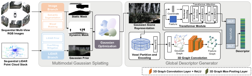
Figure 2: The overall architecture of GSPR. Multimodal Gaussian Splatting employs strategies including LiDAR-based Gaussian initialization and mixed masking mechanism to fuse LiDAR and camera data into a spatio-temporal unified MGS scene representation. The Global Descriptor Generator voxelizes the MGS scene representation and employs 3D graph convolution and transformer to extract high-level local and global spatio-temporal features embedded within the scene. Finally, the high-level spatio-temporal features are aggregated into place recognition descriptors using NetVLAD-MLPs combos.

II-C 3D Gaussian Splatting for Autonomous Driving

3D-GS performs well in static, bounded small scenes, but faces limitations such as scale uncertainty and training view overfitting in autonomous driving scenarios. To address these challenges, Yan et al. [23] propose Street Gaussian, which uses LiDAR point prior and introduces 4D spherical harmonics to represent dynamic objects. Zhou et al. [24] introduce Driving Gaussian, integrating an incremental static Gaussian model with a composite dynamic Gaussian graph for scene reconstruction. Following this, S3Gaussian, proposed by Huang et al. [25], attempts to eliminate the reliance on annotated data by introducing a multi-resolution hex plane for self-supervised foreground-background decomposition. DHGS proposed by Shi et al. [26] uses a signed distance field to supervise the geometric attributes of road surfaces. Inspired by these works, we propose Multimodal Gaussian Splatting, leveraging multimodal data and the proposed mixed masking mechanism, to provide stable and geometrically accurate reconstruction results of autonomous driving scenes for place recognition.

III Our Approach

The overview of our proposed GSPR is depicted in Fig. 2. GSPR is composed of two components: Multimodal Gaussian Splatting (MGS) and Global Descriptor Generator (GDG). Multimodal Gaussian Splatting fuses the multi-view camera and LiDAR data into a spatio-temporally unified Gaussian scene representation. Global Descriptor Generator extracts high-level spatio-temporal features from the scene through 3D graph convolution and transformer module, and aggregates the features into discriminative global descriptors for place recognition.

III-A Multimodal Gaussian Splatting

As illustrated in Fig. 3, we introduce Multimodal Gaussian Splatting for autonomous driving scene reconstruction. The method processes multimodal data through the Image Branch and the LiDAR Branch, and then integrates different modalities into a spatio-temporally unified explicit scene representation through Gaussian Optimization. The Image Branch utilizes sequential multi-view RGB images as input, generating dynamic and static masks through the mixed masking mechanism. The LiDAR Branch complements the LiDAR coverage of distant landscapes to mitigate overfitting, and provide a LiDAR prior for the initialization of Gaussians.

III-A1 LiDAR Prior

The vanilla 3D-GS uses SfM to reconstruct point clouds for initializing the Gaussian model. However, in autonomous driving scenarios, SfM can fail due to the complexity of the scene, illumination changes, and the high-speed movement of the ego vehicle. To address this, we introduce LiDAR point clouds for initializing the position of Gaussians following [23, 24]. Using LiDAR point as position prior, the distribution of 3D Gaussian can be represented as:

$$f(\mathbf{x}|\mu^{\scriptscriptstyle\text{L}},\Sigma)=e^{-\frac{1}{2}(\mathbf{x}-\mu^{\scriptscriptstyle\text{L}})^{\mathrm{T}}\Sigma^{-1}(\mathbf{x}-\mu^{\scriptscriptstyle\text{L}})}$$ (1)

where $\mu^{\scriptscriptstyle\text{L}}\in\mathbb{R}^{3}$ is the position of the LiDAR point, $\Sigma\in\mathbb{R}^{3\times 3}$ is the covariance matrix of the 3D Gaussian.

To fully utilize the spatio-temporal consistency between different modalities during the Gaussian initialization, we employ RGB images to perform LiDAR point cloud coloring. This approach provides a prior for initializing the spherical harmonic coefficients of the Gaussians. To obtain accurate correspondences between LiDAR points $(x^{\scriptscriptstyle\text{L}},y^{\scriptscriptstyle\text{L}},z^{\scriptscriptstyle\text{L}})^{\mathrm{T}}\in\mathbb{R}^{3}$ and pixels $(u,v)^{\mathrm{T}}\in\mathbb{R}^{2}$, we segment the LiDAR points that fall within the frustum of each training view and subsequently project these points onto the pixel coordinate of the corresponding image to obtain RGB values:

$$C^{p_{i}^{\scriptscriptstyle\text{L}}}_{\text{rgb}}=\mathrm{Interpolate}\left(I,K_{\text{intr}}(Rp_{i}^{\scriptscriptstyle\text{L}}+t)\right),p_{i}^{\scriptscriptstyle\text{L}}\in F$$ (2)

where $C^{p_{i}^{\scriptscriptstyle\text{L}}}_{\text{rgb}}$ is the corresponding color of LiDAR point $p_{i}^{\scriptscriptstyle\text{L}}$, $I$ represents the image, $K_{\text{intr}}$ and $R$ are the intrinsic parameters and extrinsic parameters of the camera corresponding to image $I$, while $F$ denotes the set of LiDAR points within the frustum of the camera.

In addition, we filter the ground points from the LiDAR point cloud and employ ground-truth annotations for object bounding box erasing, in order to ensure high-quality reconstruction of the static background.

III-A2 Overfitting Mitigation

Unlike bounded scenarios that the vanilla 3D-GS can trivially render, autonomous driving scenes present challenges due to their boundlessness and sparse distribution of training views. This scarcity of supervision signals results in overfitting of training views, leading to floating artifacts and misalignment of geometric structures.

An important cause of overfitting is the confusion between near and distant scenes. Due to insufficient geometric information on distant landscapes, the Gaussians are prone to fit distant scenes as floating artifacts in near scenes during the training process, leading to background collapse. Referring to the strategy employed in [27] for sky reconstruction, we mitigate this effect by adding spherical $\mathcal{P}_{\text{s}}$, composed of a set of points uniformly distributed along the periphery of the LiDAR point cloud. This operation aims to enhance the reconstruction quality of distant scenes beyond the LiDAR coverage. The spherical is also colored through multi-view RGB images to serve as the initial Gaussian prior.

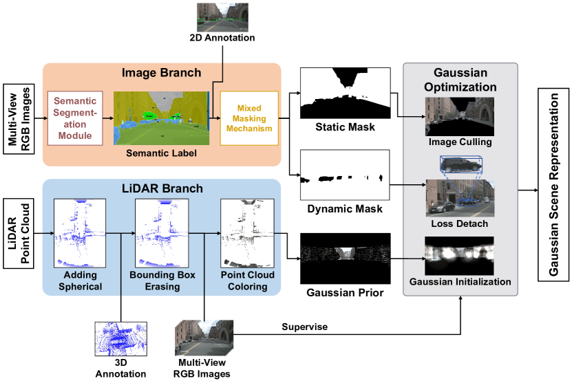
Figure 3: The pipeline of Multimodal Gaussian Splatting. Processed LiDAR point clouds supply prior information for initializing the Gaussian model. RGB image sequences are utilized to generate distinct masks that supervise the Gaussian optimization process, following semantic segmentation and mixed masking mechanism. After iterative Gaussian optimization, the multimodal data are integrated into a unified MGS scene representation.

III-A3 Mixed Masking Mechanism

In autonomous driving scenes, there are environmental features that exhibit instability over time and contain less valuable information for place recognition. Therefore, we propose the mixed masking mechanism focusing on reconstructing only the stable parts during the Gaussian optimization process.

We employ Mask2Former [28], pre-trained on the Cityscapes dataset [29], as our semantic segmentation module to generate semantic labels for the training images. By integrating semantic labels with 2D ground-truth annotations, we can obtain instance-level mask representations. In light of the nature of unstable environmental features, we categorize the masked regions into static masks (e.g., sky and road surfaces) and dynamic masks (e.g., vehicles and pedestrians), each playing distinct roles during the Gaussian optimization process. The static masks are utilized as a criterion for training image culling. Areas of the training images covered by the static masks are overlaid with the background color of the 3D-GS renderer, serving to restrict the generation of Gaussians. Conversely, the dynamic masks encompass dynamic objects within the scenarios. Notably, directly culling the shadow areas of these dynamic objects may result in unnecessary information loss. Therefore, we adopt a loss detach strategy, omitting the $\mathcal{L}_{\text{MGS}}$ loss [9] (see Eq. (10)) for the masked regions during the Gaussian optimization process. This strategy mitigates the negative effects of dynamic objects and simultaneously maintains enough supervision for large-scale reconstruction compared to directly filtering out frames with dynamic objects.

As demonstrated in Fig. 4, our proposed mixed masking mechanism effectively masks out unstable features. Additionally, the employment of LiDAR prior and the adaption of overfitting mitigation techniques contribute to maintaining a consistent scale and accurate geometric structure of the reconstructed scene. Consequently, our proposed MGS exhibits enhanced novel view synthesis capabilities compared to the vanilla 3D-GS in autonomous driving scenarios, providing MGS scene representations with spatio-temporal consistency to describe places.

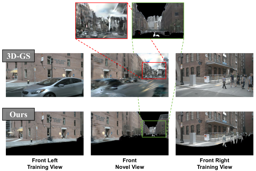
Figure 4: A comparison of the rendering results between our MGS and the vanilla 3D-GS. The environmental features of lesser significance for place recognition are masked, while the integration of LiDAR prior enhances the geometric accuracy of explicit scene reconstruction.

III-B Global Descriptor Generator

Global Descriptor Generator is used to extract distinctive place recognition descriptors from the proposed MGS representations. To extract the high-level spatio-temporal features, we first voxelize the MGS scene, and then extract local and global features through a backbone network composed of 3D graph convolutions [30] and transformer [31] module. Finally, the spatio-temporal features are fed into NetVLAD-MLPs combos [4] and aggregated into discriminative descriptors.

III-B1 Voxel Partition and Encoding

To tackle the disordered distribution of Gaussians, we first organize the MGS scene into a form that facilitates feature extraction through voxelization. Denote $\mathcal{G}=\{g_{m}=[x_{m}^{\scriptscriptstyle\text{G}},y_{m}^{\scriptscriptstyle\text{G}},z_{m}^{\scriptscriptstyle\text{G}},s_{m},q_{m},sh_{m},\alpha_{m}]^{\mathrm{T}}\in\mathbb{R}^{59}\}_{m=1...M}$ as a MGS scene, where $g_{m}$ represents the $m$-th Gaussian in the scene, $x_{m}^{\scriptscriptstyle\text{G}},y_{m}^{\scriptscriptstyle\text{G}},z_{m}^{\scriptscriptstyle\text{G}}$ denote the position of the Gaussian, $s_{m}$ means the scale matrix, $q_{m}$ is the quaternion, $sh_{m}$ means the SH coefficents, and $\alpha_{m}$ denotes the opacity. Inspired by [32], we subdivide the space into voxels in cylindrical coordinates, to ensure the uniformity of the partitioning of the Gaussian model. Considering the position property of the Gaussians, we allocate them to the corresponding voxels using the voxel partition implementation of [33], converting the Gaussian model with sizes of $M\times 59$ to $N\times H\times 59$, where $N$ is the number of voxels, and $H$ is the maximum number of Gaussians within each voxel.

Let $\mathcal{V}=\{g_{h}=[x_{h}^{\scriptscriptstyle\text{G}},y_{h}^{\scriptscriptstyle\text{G}},z_{h}^{\scriptscriptstyle\text{G}},s_{h},q_{h},sh_{h},\alpha_{h}]^{\mathrm{T}}\in\mathbb{R}^{59}\}_{h=1...H}$ as a non-empty voxel containing $H$ Gaussians, we use MeanVFE [34] to encode the voxel feature to ensure the real-time performance and usability of the network:

$$\overline{\mathcal{V}}=\{\frac{\sum\limits_{h=1}^{H}\mu_{h}^{\scriptscriptstyle\text{G}}}{H},\frac{\sum\limits_{h=1}^{H}s_{h}}{H},\frac{\sum\limits_{h=1}^{H}q_{h}}{H},\frac{\sum\limits_{h=1}^{H}sh_{h}}{H},\frac{\sum\limits_{h=1}^{H}\alpha_{h}}{H}\}$$ (3)

where $\overline{\mathcal{V}}$ denotes the encoded voxel, and $\mu^{\scriptscriptstyle\text{G}}_{h}$ means the position $(x_{h}^{\scriptscriptstyle\text{G}},y_{h}^{\scriptscriptstyle\text{G}},z_{h}^{\scriptscriptstyle\text{G}})$ of the $h$-th Gaussian in the voxel. After the voxel encoding operation, the voxel set of shape $N\times H\times 59$ is encoded into an input form of $N\times 59$. We denote the encoded MGS scene representation as $\overline{\mathcal{G}}=\{\overline{g}_{n}=[\overline{x}_{n}^{\scriptscriptstyle\text{G}},\overline{y}_{n}^{\scriptscriptstyle\text{G}},\overline{z}_{n}^{\scriptscriptstyle\text{G}},\overline{s}_{n},\overline{q}_{n},\overline{sh}_{n},\overline{\alpha}_{n}]^{\mathrm{T}}\in\mathbb{R}^{59}\}_{n=1...N}$. Ultimately, the voxel downsampling operation imparts orderliness to the Gaussian scene and reduces the number of Gaussians that need to be processed.

III-B2 3D Graph Convolution

Inspired by the successful application of graph convolution in place recognition [35, 15], we use a 3D-GCN-based [30] graph convolution backbone network to fully exploit the local features in the scene.

Based on the encoded MGS scene representation $\overline{\mathcal{G}}$, we construct a Gaussian graph according to the spatial relationships within it, using $p_{\text{gs}}=\{\overline{x}^{\scriptscriptstyle\text{G}},\overline{y}^{\scriptscriptstyle\text{G}},\overline{z}^{\scriptscriptstyle\text{G}}\}\in\mathbb{R}^{3}$ as the graph node’s coordinate and $\bm{f}(p_{\text{gs}})=\{\overline{s},\overline{q},\overline{sh},\overline{\alpha}\}\in\mathbb{R}^{56}$ as the node’s feature vector. To extract the local features of each node $p_{\text{gs}}^{n}$, we use kNN to construct the receptive field $R_{n}^{J}$ of $p_{\text{gs}}^{n}$ in 3D graph structure:

$$R_{n}^{J}=\left\{p_{\text{gs}}^{n},p_{\text{gs}}^{j}|\forall p_{\text{gs}}^{j}\in\mathcal{N}\left(p_{\text{gs}}^{n},J\right)\right\}$$ (4)

where $\mathcal{N}(.)$ denote the nearest neighbors operation using Euclidean distance, $J$ means the predefined number of neighbors, and $p_{\text{gs}}^{j}$ is the $j$-th neighbor of $p_{\text{gs}}^{n}$.

Additionally, we follow the definition in 3D-GCN, representing the 3D graph convolution kernel $K^{S}$ as a combination of unit support vectors with the origin as the starting point and their associated weights:

$$K^{S}=\left\{\bm{w}(k_{\text{C}}),\left(k_{s},\bm{w}(k_{s})\right)|s=1,2,...S\right\}$$ (5)

where $k_{\text{C}}$ is the center of the kernel, $k_{s}$ are the support vectors, $\bm{w}(k)$ denote the associated weights, and $S$ is the number of the support vectors in the kernel. Thus, we can define the 3D-GCN graph convolution operation $Conv(R_{n}^{J},K^{S})$ as:

$$\begin{split}Conv(R_{n}^{J},K^{S})&=\langle\bm{f}(p_{\text{gs}}^{n}),\bm{w}(k_{\text{C}})\rangle\\ &+\sum\limits_{s=1}^{S}\mathop{\max}_{j\in(1,J)}\left\{sim(p_{\text{gs}}^{j},k_{s})\right\}\end{split}$$ (6)

$$sim(p_{\text{gs}}^{j},k_{s})=\langle\bm{f}(p_{\text{gs}}^{j}),\bm{w}(k_{s})\rangle\frac{\langle d_{j,n},k_{s}\rangle}{||d_{j,n}||\cdot||k_{s}||}$$ (7)

We perform zero-mean normalization on the coordinates of the Gaussian graph and subsequently feed the Gaussian graph into stacked 3D graph convolution layers, 3D graph max-pooling layers [30], and ReLU nonlinear activation layers. The graph convolution backbone network generates output feature graph $F^{\text{out}}\in\mathbb{R}^{B\times N_{\text{out}}\times CH}$ based on the input features of Gaussian graph $F^{\text{in}}\in\mathbb{R}^{B\times N\times 56}$, which are then used for subsequent processing, where $B$ means the batch size, and $CH$ denotes the output channel dimension. The use of graph convolution enhances the network’s ability to aggregate local spatio-temporal features within the Gaussian graph, contributing to the discriminativity of place recognition representations.

III-B3 Transformer Module

We use transformers following the previous works [36, 6] to boost place recognition performance. Compared to these works that focus primarily on self-attention mechanisms without incorporating positional embedding, we propose using a learnable positional embedding to integrate spatial correlations from the feature graph into the latent feature space of the transformer.

The architecture of the transformer module is depicted in Fig. 5. To enable the transformer to capture the spatial correlations embedded in the feature graph, we explicitly encode the coordinates of the feature graph $p_{\mathrm{feat}}^{i}$ using learnable positional embedding:

$$\bm{r}_{i}=\mathrm{MLP}\left(\mathrm{ReLU}\left(\mathrm{MLP}(p_{\text{feat}}^{i})\right)\right)$$ (8)

where $\bm{r}_{i}$ is the positional embedding of feature $\bm{f}(p_{\text{feat}}^{i})$.

After adding the positional embeddings to the features and performing feature fusion through 3D graph convolution layers, we feed the position-encoded features into multi-head attention to fully extract the global spatio-temporal information in the scene. The self-attention mechanism can be formulated as:

$$\mathcal{A}=\mathrm{Attention}(Q,K,V)=\mathrm{softmax}\left(\frac{QK^{\mathrm{T}}}{\sqrt{d_{\text{k}}}}\right)V$$ (9)

where $\mathcal{A}$ denotes the feature with global context, $Q,K,V$ represent the queries, keys and values respectively, and $d_{\text{k}}$ is the dimension of keys.

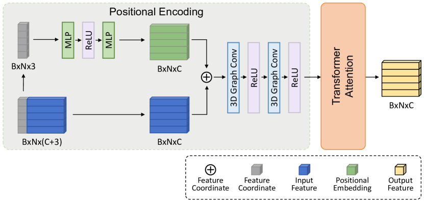
Figure 5: The detailed architecture of transformer module. Feature coordinates are explicitly encoded as positional embeddings and fused with features through graph convolutions. A transformer attention is used to extract global context from the features.

TABLE I: Comparision of place recognition performance on the BS, SON and SHV split

Methods	Sequence1	Modality2	BS split			SON split			SQ split
			AR@1	AR@5	AR@10	AR@1	AR@5	AR@10	AR@1	AR@5	AR@10
NetVLAD [2]	$\times$	V	69.94	78.51	83.57	73.42	83.04	87.09	67.28	79.20	83.49
OverlapTransformer [6]	$\times$	L	66.62	86.26	89.76	78.03	94.19	97.22	77.13	95.12	97.26
MinkLoc++ [7]	$\times$	V+L	74.19	90.04	92.99	86.62	96.46	97.98	88.11	94.21	95.12
LCPR [8]	$\times$	V+L	71.25	84.99	88.92	90.40	97.73	98.48	74.09	89.33	92.38
SeqNet [37]	$\checkmark$	V	74.86	83.29	87.78	87.09	92.66	95.19	78.59	86.85	88.99
OT+SeqNet [6, 37]	$\checkmark$	L	72.61	87.50	91.29	90.38	97.47	98.73	93.88	98.47	98.78
SeqOT [17]	$\checkmark$	L	78.68	89.76	93.41	94.70	98.23	98.74	96.34	98.48	99.39
Autoplace [16]	$\checkmark$	R	83.85	93.12	95.93	95.70	98.73	99.24	95.72	98.78	98.78
GSPR (ours)	$\checkmark$	V+L	97.05	99.16	99.72	97.22	99.49	99.75	96.95	99.09	99.70
1 Use sequential data. 2 V: Visual, L: LiDAR, R: Radar, V+L: Visual+LiDAR.

III-C Two-step Training Strategy

We adopt a two-stage process to train the GSPR. First, we train explicit representations of autonomous driving scenes based on Multimodal Gaussian Splatting. Subsequently, the Global Descriptor Generator is trained for place recognition using the generated MGS scene representations.

Following 3D-GS [9], we supervise the Gaussian optimization process of Multimodal Gaussian Splatting using the combination of the Mean Absolute Error loss $\mathcal{L}_{1}$ and the Structural Similarity Index Measure loss $\mathcal{L}_{\text{D-SSIM}}$:

$$\begin{split}\mathcal{L}_{\text{MGS}}\left(I_{\text{render}},I_{\text{gt}}\right)&=(1-\lambda)\mathcal{L}_{1}\left(I_{\text{render}},I_{\text{gt}}\right)\\ &+\lambda\mathcal{L}_{\text{D-SSIM}}\left(I_{\text{render}},I_{\text{gt}}\right)\end{split}$$ (10)

where $I_{\text{render}}$ is the image rendered by the 3D-GS renderer from the MGS scene representation, and $I_{\text{gt}}$ represents the ground-truth image. By evaluating the differences between the rendered image and the ground-truth image, we supervise the updates of Gaussian attributes and adjust the Gaussian distribution density. This process enables the iterative refinement of an accurate MGS scene representation of the real autonomous driving scenario.

To supervise the Global Descriptor Generator, we employ the contrastive learning scheme. For each query descriptor $\mathcal{D}$ representing an MGS scene representation, we choose $k_{\text{pos}}$ positive descriptors $\left\{\mathcal{D}_{\text{pos}}\right\}$ and $k_{\text{neg}}$ negative descriptors $\left\{\mathcal{D}_{\text{neg}}\right\}$ to construct a triplet $\mathcal{T}=\left(\mathcal{D},\left\{\mathcal{D}_{\text{pos}}\right\},\left\{\mathcal{D}_{\text{neg}}\right\}\right)$. Following previous works [16, 8], we define samples within 9 meters of the query sample as positive, otherwise negative. We input the triplets into lazy triplet loss [4] to compute the loss, accelerating network convergence and boosting place recognition performance through mini-batch hard mining. The loss function is given by:

$$\mathcal{L}_{\text{GDG}}(\mathcal{T})\!=\!\left[\beta\!+\!\mathop{\min}_{o}(d(\mathcal{D}\!,\mathcal{D}_{\text{pos}}^{o}))\!-\!\mathop{\max}_{a}(d(\mathcal{D}\!,\mathcal{D}_{\text{neg}}^{a}))\right]_{+}$$ (11)

where $\left[\cdots\right]_{+}$ denotes the hinge loss, $d(\cdot)$ is the Euclidean distance between a pair of descriptors, and $\beta$ is the margin.

IV Experiments

IV-A Experimental Setup and Implementation Details

We use nuScenes dataset [38] to evaluate our method, which consists of autonomous driving scenes collected from four different locations in Boston and Singapore: Boston Seaport (BS), SG-OneNorth (SON), SG-Queenstown (SQ), and SG-HollandVillage (SHV). The dataset provides multimodal data from 32-beam LiDAR and multi-view cameras, as well as rich 3D object annotations, facilitating scene reconstruction and allowing for comprehensive evaluation of place recognition methods. To obtain statistically significant results, we conduct experiments on the BS, SON, and SQ splits, which have sufficient loop closures and diverse situations.

We design the data preparation pipeline following previous works [16, 8], with some modifications. Specifically, we divide the data into the trainval set and the test set according to data collection time, and extract train query set and val query set from the trainval set, and test query set from the test set. We decrease the place density of the global map to 3 meters, and the place density of the query frames to 9 meters, thus widening the gap between viewpoints and raising the difficulty of place recognition. Additionally, both the database set and the training query set are utilized as query frames to ensure that the training set contains a sufficient number of triplets.

For the Multimodal Gaussian Splatting module, we set the training iterations to 4000, the densification interval to 200, and stop densifying within 2000 iterations. This configuration is employed to reduce the training time of MGS and regulate the number of Gaussians. For the 3D graph convolution backbone, we set the number of neighbors $J=25$, the kernel support number $S=1$, and the sampling rate of the 3D graph max-pooling $r_{\text{pool}}=0.25$. For the transformer module, we set the positional embedding and the feature embedding dimension $d_{\text{pe}}=d_{\text{model}}=512$, the feed-forward dimension $d_{\text{ffn}}=1024$, and the number of heads $n_{\text{head}}=8$. For the NetVLAD module, we set the number of clusters $d_{\text{cluster}}=64$, and the output dimension $d_{\text{out}}=256$. An ADAM optimizer is used to train the network, while the initial learning rate is set to $1\times 10^{-7}$ and decays by a factor of 0.5 every 5 epochs. For the lazy triplet loss, we set the number of positive samples $k_{\text{pos}}=2$, the number of negative samples $k_{\text{neg}}=6$, and the margin $\beta=0.5$.

IV-B Evaluation for Place Recognition

To validate the place recognition performance of GSPR in large-scale outdoor environments, we compare it with state-of-the-art baseline methods, including the visual-based methods NetVLAD [2] and SeqNet [37], the LiDAR-based methods OverlapTransformer [6], SeqNet-enhanced OverlapTransformer, and SeqOT [17], the radar-based method Autoplace [16], and the multimodal methods MinkLoc++ [7] and LCPR [8]. Among these, SeqNet [37], SeqNet-enhanced OverlapTransformer, SeqOT [17], and Autoplace [16] use sequential observations as inputs, compared to the other baselines only using one single frame for each retrieval. All experiments are conducted on a system with an Intel i7-14700KF CPU and an Nvidia RTX 4060Ti GPU.

We first train and test GSPR and the baseline methods on the largest BS split, and use the pretrained weights to perform zero-shot generalization experiments on the SON and SQ splits. We set the sequence length for all sequence-enhanced place recognition methods to 3 for evaluation fairness.

Following previous works [16, 18], we use average top 1 recall (AR@1), top 5 recall (AR@5), and top 10 recall (AR@10) as metrics to evaluate place recognition performance, with results presented in Tab. I. Our proposed GSPR outperforms all baselines on the BS, SON, and SQ splits, which include challenging conditions such as rain and nighttime. This demonstrates that our method effectively handles scenarios where unimodal approaches often fall short. Additionally, zero-shot generalization experiments on the SON and SQ splits indicate that our method achieves cross-scene and long-term generalization capability with limited training data.

IV-C Study on Maximum Sampling Range

We conduct an ablation study to investigate the impact of varying the maximum sampling range during voxel partitioning on GSPR’s place recognition performance. This study aims to evaluate the contribution of Gaussians distributed at different distances within the scene. The experimental results on the BS split are presented in Fig. 6. As can be observed, the best place recognition performance occurs when the maximum sampling distance is at least 40 meters. Notably, the AR@1 does not significantly improve with sampling range increase after 40 meters. A possible reason is that each Gaussian scene is initialized from LiDAR data where points at greater distances are more sparse, leading to less distinct spatio-temporal features to boost the recognition performance.

TABLE II: The impact of different voxel numbers

Voxel Number	AR@1	AR@5	AR@10	AR@20	Inference Time [ms]
1024	72.09	91.58	95.93	97.76	4.32
2048	88.22	97.62	98.88	99.72	4.52
4096	96.77	98.60	99.16	99.16	11.76
8192	97.05	99.16	99.72	99.72	41.02

IV-D Study on Number of Voxels

In our experimental setup, each scene consists of approximately 100,000 Gaussians. To organize the unordered Gaussian scene and mitigate computational load, we downsample it into a set of $N$ voxels using voxel partitioning. Inspired by the LiDAR downsampling algorithm in PointNetVLAD [4], we adaptively adjust voxel size to transform all Gaussian scenes into $N$ voxels. A larger $N$ preserves fine details but incurs higher computational costs, while a smaller $N$ increases inference speed at the cost of information loss. To assess the impact of voxel count $N$ on place recognition performance, we conduct experiments on the BS split. As shown in Tab. II, setting $N$ to 4096 achieves a balance between performance and inference speed, as very low voxel counts result in significant information loss, while excessively high counts lead to impractical computational demands.

TABLE III: Ablation study of input features on the BS split

SH	Opacity	Rotation	Scale	Position	AR@1	AR@5	AR@10
✓					64.38	81.91	86.54
✓	✓				73.63	88.50	93.41
✓	✓	✓			73.77	89.06	93.55
✓	✓	✓	✓		86.26	96.91	98.32
✓	✓	✓	✓	✓	97.05	99.16	99.72

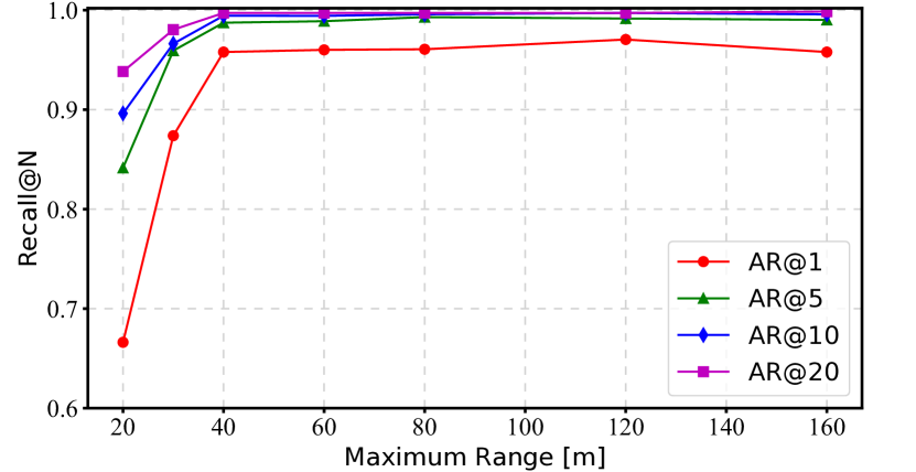
Figure 6: The impact of maximum sampling distance on place recognition performance.

IV-E Ablation Study on Input Features

A Gaussian $g=[\mu^{\scriptscriptstyle\text{G}},s,q,sh,\alpha]\in\mathbb{R}^{59}$ is composed of different parts of features, including position $\mu^{\scriptscriptstyle\text{G}}\in\mathbb{R}^{3}$, scale $s\in\mathbb{R}^{3}$, rotation $q\in\mathbb{R}^{4}$, SH coefficients $sh\in\mathbb{R}^{48}$, and opacity $\alpha\in\mathbb{R}^{1}$. In GSPR, position is fed into the transformer module as positional encoding, while scale, rotation, SH coefficients, and opacity are input features of the graph convolution backbone network. We conduct an ablation study on input features using the BS split to examine the impact of different components of the Gaussian on place recognition performance. The results are shown in Tab. III. As can be seen, in addition to the SH coefficients, the Gaussian features of position, scale, and opacity provide valuable information for place recognition, while the rotation feature contributes relatively less. This suggests that ”where it is” is more expressive than ”which direction it is heading” for Gaussian-based place description, as the former corresponds more directly to the explicit spatial structure of the places.

V Conclusion

In this paper, we present GSPR, a novel multimodal place recognition network based on 3D-GS. Our method proposes Multimodal Gaussian Splatting to harmonize continuous observations, including multi-view RGB images and LiDAR point clouds, creating a spatio-temporal unified MGS scene representation tailored for autonomous driving scenarios. To manage the unordered Gaussians, we implement voxel downsampling for effective organization. We further propose using 3D graph convolution networks and transformer module to exploit local and global spatio-temporal features from Gaussian graphs, generating discriminative descriptors for place recognition. The experimental results suggest that our method outperforms state-of-the-art baselines, including unimodal, multimodal, and sequence-enhanced methods. It demonstrates the advantages of the 3D-GS-based multimodal fusion approach in handling challenging place recognition tasks with notable generalization ability.

References

- [1] Relja Arandjelovic and Andrew Zisserman. All about vlad. In Proceedings of the IEEE conference on Computer Vision and Pattern Recognition, pages 1578–1585, 2013.
- [2] Relja Arandjelovic, Petr Gronat, Akihiko Torii, Tomas Pajdla, and Josef Sivic. Netvlad: Cnn architecture for weakly supervised place recognition. In Proceedings of the IEEE conference on computer vision and pattern recognition, pages 5297–5307, 2016.
- [3] Stephen Hausler, Sourav Garg, Ming Xu, Michael Milford, and Tobias Fischer. Patch-netvlad: Multi-scale fusion of locally-global descriptors for place recognition. In Proceedings of the IEEE/CVF Conference on Computer Vision and Pattern Recognition, pages 14141–14152, 2021.
- [4] Mikaela Angelina Uy and Gim Hee Lee. Pointnetvlad: Deep point cloud based retrieval for large-scale place recognition. In Proceedings of the IEEE conference on computer vision and pattern recognition, pages 4470–4479, 2018.
- [5] Jacek Komorowski. Minkloc3d: Point cloud based large-scale place recognition. In Proceedings of the IEEE/CVF Winter Conference on Applications of Computer Vision, pages 1790–1799, 2021.
- [6] Junyi Ma, Jun Zhang, Jintao Xu, Rui Ai, Weihao Gu, and Xieyuanli Chen. Overlaptransformer: An efficient and yaw-angle-invariant transformer network for lidar-based place recognition. IEEE Robotics and Automation Letters, 7(3):6958–6965, 2022.
- [7] Jacek Komorowski, Monika Wysoczańska, and Tomasz Trzcinski. Minkloc++: lidar and monocular image fusion for place recognition. In 2021 International Joint Conference on Neural Networks (IJCNN), pages 1–8. IEEE, 2021.
- [8] Zijie Zhou, Jingyi Xu, Guangming Xiong, and Junyi Ma. Lcpr: A multi-scale attention-based lidar-camera fusion network for place recognition. IEEE Robotics and Automation Letters, 2023.
- [9] Bernhard Kerbl, Georgios Kopanas, Thomas Leimkühler, and George Drettakis. 3d gaussian splatting for real-time radiance field rendering. ACM Trans. Graph., 42(4):139–1, 2023.
- [10] Michael J Milford and Gordon F Wyeth. Seqslam: Visual route-based navigation for sunny summer days and stormy winter nights. In 2012 IEEE international conference on robotics and automation, pages 1643–1649. IEEE, 2012.
- [11] Yunge Cui, Xieyuanli Chen, Yinlong Zhang, Jiahua Dong, Qingxiao Wu, and Feng Zhu. Bow3d: Bag of words for real-time loop closing in 3d lidar slam. IEEE Robotics and Automation Letters, 8(5):2828–2835, 2023.
- [12] Jun Yu, Chaoyang Zhu, Jian Zhang, Qingming Huang, and Dacheng Tao. Spatial pyramid-enhanced netvlad with weighted triplet loss for place recognition. IEEE transactions on neural networks and learning systems, 31(2):661–674, 2019.
- [13] Sijie Zhu, Linjie Yang, Chen Chen, Mubarak Shah, Xiaohui Shen, and Heng Wang. R2former: Unified retrieval and reranking transformer for place recognition. In Proceedings of the IEEE/CVF Conference on Computer Vision and Pattern Recognition, pages 19370–19380, 2023.
- [14] Sergio Izquierdo and Javier Civera. Optimal transport aggregation for visual place recognition. In Proceedings of the IEEE/CVF Conference on Computer Vision and Pattern Recognition, pages 17658–17668, 2024.
- [15] Le Hui, Hang Yang, Mingmei Cheng, Jin Xie, and Jian Yang. Pyramid point cloud transformer for large-scale place recognition. In Proceedings of the IEEE/CVF International Conference on Computer Vision, pages 6098–6107, 2021.
- [16] Kaiwen Cait, Bing Wang, and Chris Xiaoxuan Lu. Autoplace: Robust place recognition with single-chip automotive radar. In 2022 International Conference on Robotics and Automation (ICRA), pages 2222–2228. IEEE, 2022.
- [17] Junyi Ma, Xieyuanli Chen, Jingyi Xu, and Guangming Xiong. Seqot: A spatial-temporal transformer network for place recognition using sequential lidar data. IEEE Transactions on Industrial Electronics, 2022.
- [18] Junyi Ma, Guangming Xiong, Jingyi Xu, and Xieyuanli Chen. Cvtnet: A cross-view transformer network for lidar-based place recognition in autonomous driving environments. IEEE Transactions on Industrial Informatics, 2023.
- [19] Xieyuanli Chen, Thomas Läbe, Andres Milioto, Timo Röhling, Jens Behley, and Cyrill Stachniss. Overlapnet: A siamese network for computing lidar scan similarity with applications to loop closing and localization. Autonomous Robots, pages 1–21, 2022.
- [20] Yuheng Lu, Fan Yang, Fangping Chen, and Don Xie. Pic-net: Point cloud and image collaboration network for large-scale place recognition. arXiv preprint arXiv:2008.00658, 2020.
- [21] Haowen Lai, Peng Yin, and Sebastian Scherer. Adafusion: Visual-lidar fusion with adaptive weights for place recognition. IEEE Robotics and Automation Letters, 7(4):12038–12045, 2022.
- [22] Jingyi Xu, Junyi Ma, Qi Wu, Zijie Zhou, Yue Wang, Xieyuanli Chen, and Ling Pei. Explicit interaction for fusion-based place recognition. arXiv preprint arXiv:2402.17264, 2024.
- [23] Yunzhi Yan, Haotong Lin, Chenxu Zhou, Weijie Wang, Haiyang Sun, Kun Zhan, Xianpeng Lang, Xiaowei Zhou, and Sida Peng. Street gaussians for modeling dynamic urban scenes. arXiv preprint arXiv:2401.01339, 2024.
- [24] Xiaoyu Zhou, Zhiwei Lin, Xiaojun Shan, Yongtao Wang, Deqing Sun, and Ming-Hsuan Yang. Drivinggaussian: Composite gaussian splatting for surrounding dynamic autonomous driving scenes. In Proceedings of the IEEE/CVF Conference on Computer Vision and Pattern Recognition, pages 21634–21643, 2024.
- [25] Nan Huang, Xiaobao Wei, Wenzhao Zheng, Pengju An, Ming Lu, Wei Zhan, Masayoshi Tomizuka, Kurt Keutzer, and Shanghang Zhang. S3gaussian: Self-supervised street gaussians for autonomous driving. arXiv preprint arXiv:2405.20323, 2024.
- [26] Xi Shi, Lingli Chen, Peng Wei, Xi Wu, Tian Jiang, Yonggang Luo, and Lecheng Xie. Dhgs: Decoupled hybrid gaussian splatting for driving scene. arXiv preprint arXiv:2407.16600, 2024.
- [27] Ke Wu, Kaizhao Zhang, Zhiwei Zhang, Shanshuai Yuan, Muer Tie, Julong Wei, Zijun Xu, Jieru Zhao, Zhongxue Gan, and Wenchao Ding. Hgs-mapping: Online dense mapping using hybrid gaussian representation in urban scenes, 2024.
- [28] Bowen Cheng, Ishan Misra, Alexander G Schwing, Alexander Kirillov, and Rohit Girdhar. Masked-attention mask transformer for universal image segmentation. In Proceedings of the IEEE/CVF conference on computer vision and pattern recognition, pages 1290–1299, 2022.
- [29] Marius Cordts, Mohamed Omran, Sebastian Ramos, Timo Scharwächter, Markus Enzweiler, Rodrigo Benenson, Uwe Franke, Stefan Roth, and Bernt Schiele. The cityscapes dataset. In CVPR Workshop on the Future of Datasets in Vision, volume 2, page 1, 2015.
- [30] Zhi-Hao Lin, Sheng-Yu Huang, and Yu-Chiang Frank Wang. Convolution in the cloud: Learning deformable kernels in 3d graph convolution networks for point cloud analysis. In Proceedings of the IEEE/CVF conference on computer vision and pattern recognition, pages 1800–1809, 2020.
- [31] A Vaswani. Attention is all you need. Advances in Neural Information Processing Systems, 2017.
- [32] Hui Zhou, Xinge Zhu, Xiao Song, Yuexin Ma, Zhe Wang, Hongsheng Li, and Dahua Lin. Cylinder3d: An effective 3d framework for driving-scene lidar semantic segmentation. arXiv preprint arXiv:2008.01550, 2020.
- [33] Spconv Contributors. Spconv: Spatially sparse convolution library. https://github.com/traveller59/spconv, 2022.
- [34] Yan Yan, Yuxing Mao, and Bo Li. Second: Sparsely embedded convolutional detection. Sensors, 18(10):3337, 2018.
- [35] Zhe Liu, Shunbo Zhou, Chuanzhe Suo, Peng Yin, Wen Chen, Hesheng Wang, Haoang Li, and Yun-Hui Liu. Lpd-net: 3d point cloud learning for large-scale place recognition and environment analysis. In Proceedings of the IEEE/CVF International Conference on Computer Vision, pages 2831–2840, 2019.
- [36] Zhicheng Zhou, Cheng Zhao, Daniel Adolfsson, Songzhi Su, Yang Gao, Tom Duckett, and Li Sun. Ndt-transformer: Large-scale 3d point cloud localisation using the normal distribution transform representation. In 2021 IEEE International Conference on Robotics and Automation (ICRA), pages 5654–5660. IEEE, 2021.
- [37] Sourav Garg and Michael Milford. Seqnet: Learning descriptors for sequence-based hierarchical place recognition. IEEE Robotics and Automation Letters, 6(3):4305–4312, 2021.
- [38] Holger Caesar, Varun Bankiti, Alex H Lang, Sourabh Vora, Venice Erin Liong, Qiang Xu, Anush Krishnan, Yu Pan, Giancarlo Baldan, and Oscar Beijbom. nuscenes: A multimodal dataset for autonomous driving. In Proceedings of the IEEE/CVF conference on computer vision and pattern recognition, pages 11621–11631, 2020.