Fisher Forecast of Finite-Size Effects with Future Gravitational Wave Detectors

Joshua Shterenberg and Zihan Zhou

Department of Physics, Princeton University, Princeton, NJ 08540, USA

  Abstract

We use Fisher information theory to forecast the bounds on the finite-size effects of astrophysical compact objects with next-generation gravitational wave detectors, including the ground-based Cosmic Explorer (CE) and Einstein Telescope (ET), as well as the space-based Laser Infrared Space Antenna (LISA). Exploiting the worldline effective field theory (EFT) formalism, we first characterize three types of quadrupole finite-size effects: the spin-induced quadrupole moments, the conservative tidal deformations, and the tidal heating. We then derive the corresponding contributions to the gravitational waveform phases for binary compact objects in aligned-spin quasi-circular orbits. We separately estimate the constraints on these finite-size effects for black holes using the power spectral densities (PSDs) of the CE+ET detector network and LISA observations. For the CE+ET network, we find that the bounds on the mass-weighted spin-independent dissipation number $\mathcal{H}_{0}$ are of the order $\mathcal{O}(1)$, while the bounds on the mass-weighted tidal Love number $\tilde{\Lambda}$ are of the order $\mathcal{O}(10)$. For high-spin binary black holes with dimensionless spin $\chi\simeq 0.8$, the bounds on the symmetric spin-induced quadrupole moment $\kappa_{s}$ are of the order $\mathcal{O}(10^{-1})$. LISA observations of supermassive black hole mergers offer slightly tighter constraints on all three finite-size parameters. Additionally, we perform a Fisher analysis for a binary neutron star merger within the CE+ET network. The bounds on the tidal parameter $\mathcal{H}_{0}$ and on $\tilde{\Lambda}$ are around two orders of magnitude better than the current LIGO-Virgo-KAGRA (LVK) bounds.

 

Email: jshteren@princeton.edu, zihanz@princeton.edu

1 Introduction

The advent of gravitational-wave (GW) astronomy, following the successful detection of GWs by the LIGO-Virgo-KAGRA (LVK) collaboration [1, 2, 3, 4, 5, 6, 7, 8, 9, 10, 11, 12, 13, 14], has significantly heightened global interest in this field over the past decade. Given the ever-increasing sensitivities of GW detectors, precise and accurate waveform modeling is crucial for deepening our understanding of the structure of compact objects [15, 16, 17, 18, 19, 20, 21]. In the early inspiral phase of mergers of compact objects, where the relative velocities of the orbiting bodies remain small, binary systems can be perturbatively described using the methods of the post-Newtonian (PN) expansion (see [22, 15, 23] for comprehensive reviews). In this framework, the binary system is initially modeled as two point particles orbiting around each other. To account for finite-size effects, one goes beyond the point-particle approximation by introducing corrections via the standard multipole expansion. At the quadrupolar level, finite-size effects in GW observables can be broadly categorized into three types: spin-induced multipole moments [24, 25, 26, 27, 28, 29, 30, 31, 32, 33], conservative tidal deformability [34, 35, 36, 37, 38, 39, 40, 41], and tidal heating [42, 43, 44, 45, 46, 47, 48, 49, 50, 51]. In this paper, we analyze the capability of future GW detectors, such as Einstein Telescope (ET) [52, 53], Cosmic Explorer (CE) [54, 55], and the Laser Interferometer Space Antenna (LISA) [56] to constrain these quadrupole finite-size effects. The former two will be treated as the CE+ET network.

In PN theories, the spin-induced quadrupole moment of a self-gravitating body arises from its rotation [57, 58, 24]. From the standpoint of PN counting, the spin-induced quadrupole moments of the binary system $\{\kappa_{1},\kappa_{2}\}$ are the dominant finite-size effects. They first appear in the phase of binary waveforms at the 2PN order [24]. For Kerr black holes (BHs), the theoretical prediction is $\kappa_{1}=\kappa_{2}=1$ [57, 58]. The first sub-leading finite-size effect is the tidal heating [42, 43, 44, 45, 46, 47, 48, 49, 50, 51, 59, 60, 61, 62] — also referred to as the tidal dissipation and characterized by the dissipation numbers $\{H_{1\omega}^{E},H_{2\omega}^{E}\}$– which appears at 2.5PN order for rotating objects and at 4PN order for spherically symmetric objects [59, 60, 61, 62]. Tidal dissipation quantifies the viscous properties of compact objects by describing the irreversible transfer of energy and angular momentum from the surrounding tidal environment into the body itself. A well-known example of this process is observed in the Earth-Moon system [50, 51, 63]. The conservative tidal deformation parameters, which first appear at 5PN order, describe the change in the density distribution and shape of a body under the influence of an external gravitational field. These deformations are characterized by the well-known “Love numbers” $\{\Lambda_{1},\Lambda_{2}\}$ [38, 39, 64, 65, 66, 67, 68, 69, 70, 71, 72, 73, 74, 12, 75, 76, 77, 78, 79]. For Kerr BHs, the Love numbers are identically zero, i.e. $\Lambda_{1}=\Lambda_{2}=0$ [67, 68, 69, 70, 71, 72, 60]. In contrast, for neutron stars (NSs), the Love numbers provide critical information that can be used to distinguish between various degrees of compactness and different equations of state (EoS) [36, 80, 81, 82], offering insight into the internal structure and composition of these compact objects.

The constraints on the spin-induced quadrupole moments and the tidal Love numbers have been studied extensively in current GW events from LVK’s observations [29, 30, 83, 84, 85, 86, 87]. For BHs, the symmetric spin-induced quadrupole moment parameter $\kappa_{s}$ is constrained to $|\kappa_{s}|\lesssim\mathcal{O}(10^{2})$ for individual events, with improvements of $|\kappa_{s}|\lesssim\mathcal{O}(10)$ at the population level [86, 87]. Similarly, the symmetric mass-weighted tidal Love number $\tilde{\Lambda}$ is constrained to $|\tilde{\Lambda}|\lesssim\mathcal{O}(10^{4})$, which is consistent with the prediction of a vanishing Love number from general relativity (GR), though far from the precision test [86, 12]. Tidal heating effects of BHs have recently been explored in data analysis [88, 61, 89]. In Ref. [61], it is shown that the symmetric mass-weighted dissipation number $\mathcal{H}_{0}$ for BHs can be constrained to $|\mathcal{H}_{0}|\lesssim 20$ at the population level. The analysis of finite-size effects for NSs requires more work because of the variety of their compactness and EoS. For spinning neutron stars with $|\chi|\lesssim 0.6$ [82], studies have shown that the spin-induced quadrupole moments $\kappa$ can vary from $2\sim 10$ depending on the EoS [90, 91]. The tidal Love number and dissipation also vary widely, from $\mathcal{O}(10^{2})$ to $\mathcal{O}(10^{4})$, again depending on the compactness and the EoS [92, 62]. Parameter estimation for both conservative and dissipative tidal effects has been applied to real data from the binary neutron star (BNS) event GW170817, yielding constraints of $\tilde{\Lambda}=300^{+420}_{-230}$ and $\mathcal{H}_{0}<1200$ at the 90% credible level [82, 88, 89].

Looking ahead, the sensitivities of next-generation gravitational wave detectors such as the ET, CE, and LISA are expected to increase dramatically compared to current detectors. ET and CE are projected to detect compact binaries in the mass range of stellar-mass BHs to roughly one hundred stellar-mass BHs, with sensitivities increased by nearly two orders of magnitude compared with the current LVK observations [52, 53, 54, 55, 93, 94]. This improvement will naturally lead to higher signal-to-noise ratios (SNRs) and tighter constraints on the finite-size effects of compact objects. LISA, on the other hand, is designed to detect gravitational waves in the millihertz range, which will enable the observation of supermassive ($10^{4}\sim 10^{7}M_{\odot}$) BBH mergers [56, 95]. These systems often involve the merger of a supermassive BH with much smaller compact objects, forming extreme-mass-ratio inspirals (EMRIs). Due to their long inspiral phases, EMRIs provide an exceptional opportunity to test GR and constrain finite-size effects in the strong-field regime. For these future detectors, some studies have already assessed the ability of carrying out such tests of GR for EMRIs and other scenarios [56, 95]. Together with the future advanced LIGO [96], advanced Virgo [97], LIGO-India [98, 99] and more, the bounds on the finite-size effects of compact objects are going to be rapidly improved both at the individual and population level.

In this paper, we follow the foundations set up by Ref. [61] and extend them to study the signature of finite-size effects of compact objects with future detectors. More specifically, we will adopt the worldline effective field theory (EFT) formalism to model the finite-size effects of compact objects and estimate the bounds on these parameters with future GW detectors. In the EFT framework [35, 100, 101, 102, 103, 104, 59, 60], all of the information about the finite-size effects is embedded in the composite operator of the quadrupole moments $Q_{ij}$. In general, $Q_{ij}$ is not known, but for spherically symmetric objects within a slowly varying external tidal environment we can exploit the time derivative expansion and linear response theory to parameterize the quadrupole moment as the following (to first order in $D_{\tau}E_{ij}$):

$$Q_{ij}^{E{\rm(tidal)}}=-m(Gm)^{4}\Bigg{[}\Lambda^{E}E_{ij}-(Gm)H_{\omega}^{E}\dfrac{D}{D\tau}E_{ij}\Bigg{]}\leavevmode\nobreak\ ,$$ (1.1)

where $\Lambda^{E}$ is the Love number and $H_{\omega}^{E}$ is the spin-independent dissipation number. The subscript $E$ denotes the parity-even electric-type tidal effects. Going beyond Newtonian gravity, one must also account for parity-odd magnetic-type tidal effects. If we extend the theory to include intrinsically rotating objects, there are two such additional contributions to the quadrupole moment [28, 63, 105, 18]:

$$Q_{ij,S}^{E{\rm(tidal)}}=-m(Gm)^{4}H_{S}^{E}\chi\hat{S}^{\langle i}{}_{k}E^{k|j\rangle}\leavevmode\nobreak\ ,\leavevmode\nobreak\ Q_{ij}^{E{\rm(spin)}}=-m(Gm\chi)^{2}\kappa\hat{S}^{i}{}_{k}\hat{S}^{k}{}_{j}\leavevmode\nobreak\ ,$$ (1.2)

where $H_{S}^{E}$ is the spin-linear dissipation number, $\kappa$ is the spin-induced quadrupole moment parameter and $\hat{S}_{ij}$ is the unit spin tensor. Previous studies have separately examined the constraining power of future detectors on spin-induced quadrupole moments and tidal Love numbers [29, 33, 106, 107, 108]. However, tidal dissipation effects have received less attention. More importantly, no analysis has yet simultaneously considered all three types of finite-size effects. In this work, we aim to fill this gap by analyzing the ability of the three aforementioned future detectors to measure the three symmetric mass-weighted finite-size parameters $\kappa_{s}$, $\mathcal{H}_{0}$, and $\tilde{\Lambda}$ for binary compact objects simultaneously.

We separately estimate the projected bounds for these parameters on the CE+ET detector network for stellar-mass BHs, and on LISA for supermassive BHs. Throughout, we adopt the electric-magnetic duality for binary black holes [109, 110, 111, 100, 112, 67, 65]. Furthermore, for the low-spin events, we use the low-spin superradiance condition to achieve better constraints for dissipation numbers (see [61] for detailed discussion). Our marginalized constraints on $\mathcal{H}_{0}$ are of the same magnitude as the theoretical predictions from GR. For high-spin events, where we do not use the superradiance condition, we get slightly less stringent constraints on the dissipation numbers, but significantly better constraints on the spin-induced quadrupole moments — about an order of magnitude tighter than the values predicted by GR. We additionally perform the Fisher analysis for the binary neutron star with the fiducial values chosen from median values of the GW170817 posterior(we set all fiducial dissipation numbers to zero) and find the 90% credible bounds on the mass-weighted tidal dissipation number to be $\mathcal{H}_{0}=0^{+1.8}_{-1.8}$, and that of the tidal Love number to be $\tilde{\Lambda}=456^{+18}_{-18}$.

Outline: The remaining structure of this paper is as follows. §2 gives a short review of the worldline EFT formalism and its modeling of the finite-size effects of compact objects. We focus on three types of finite-size effects: spin-induced quadrupole moments, conservative tidal deformation, and tidal heating. We then derive our corresponding IMRPhenomD+FiniteSize waveform to capture the imprints of these finite-size effects on GW waveforms. §3 presents our Fisher forecasting of the projected bounds on the three finite-size effects mentioned above. In §4, we first summarize our results. Then we identify possible systematic errors in our waveform modeling and give some outlook on future research directions. The Appendix complements §2 in further detailing the derivations for the waveform observables used.

Notations and Conventions: We use the natural units $G=c=1$ unless otherwise specified. We use the $(-+++)$ metric signature, with Greek letters for covariant indices and Latin letters for indices within local tetrads. We use $m_{\ell}$ to denote the azimuthal angular momentum to avoid confusion with the component mass $m$. We adopt the following conventions for several convenient mass and spin quantities:

$$M :=m_{1}+m_{2}\,\qquad\eta:=m_{1}m_{2}/M^{2}\,\qquad\delta:=\left(m_{1}-m_{2}\right)/M$$ (1.3)

$$\chi_{i} :=\mathbf{S}_{i}/m_{i}^{2}\,\qquad\bm{\chi}_{s}:=\left(\bm{\chi}_{1}+\bm{\chi}_{2}\right)/2\,\qquad\bm{\chi}_{a}:=\left(\bm{\chi}_{1}-\bm{\chi}_{2}\right)/2$$

where $\mathbf{S}_{i}$ is the component spin angular momentum vector and $\chi_{i}$ is the dimensionless spin. The mass-weighted symmetrized versions of various finite-size parameters are defined in Eqs. (2.11).

2 Finite-Size Effects on Gravitational Waves

2.1 Short Review: EFT Formalism with Finite-Size Effects

The theoretical basis surrounding our work is the worldline effective field theory (EFT) formalism of gravitational compact objects, which has been extensively studied in the literature [100, 25, 112, 104, 113, 114]. The construction of the EFT is based on the multipole expansion approach, where the higher order terms are designed to capture more detailed information about the system. The leading order term of the EFT describes the compact objects as point particles. More specifically, the point-particle degrees of freedom are captured by the four velocity $u^{\mu}$ of the worldline. When going beyond this point-particle limit, we use the multipole expansion to account for the fine structure within the compact object. In this paper, we will only focus on the quadrupole terms. Let us denote the co-moving four-tetrads as $e_{i}^{\mu};i\in\{0,1,2,3\}$. Within the external gravitational field $g_{\mu\nu}$, one can write down the effective action of the system as

$$S=\int d\tau\Bigg{[}-m+\mathcal{L}(Q_{ij}^{E/B},\dot{Q}_{ij}^{E/B})-\dfrac{1}{2}Q_{ij}^{E}E^{ij}-\dfrac{1}{2}Q_{ij}^{B}B^{ij}\Bigg{]}\leavevmode\nobreak\ ,$$ (2.1)

where $m$ is the mass of the compact object and $Q_{ij}$ is the quadrupole moment. Here, the external electric and magnetic fields $E_{ij}$ and $B_{ij}$ are defined as

$$E_{ij}=C_{\mu\rho\nu\sigma}u^{\rho}u^{\sigma}e_{i}^{\mu}e_{j}^{\nu};\qquad B_{ij}=u^{\mu}e_{i}^{\nu}u^{\rho}e_{j}^{\sigma}{}^{*}C_{\mu\nu\rho\sigma}\leavevmode\nobreak\ ,$$ (2.2)

where $C_{\mu\nu\rho\sigma}$ is the Weyl tensor of the external gravitational field and ${}^{*}C_{\mu\nu\rho\sigma}$ stands for its dual. Once we treat $Q_{ij}$ as a dynamical variable, the Lagrangian $\mathcal{L}(Q_{ij},\dot{Q}_{ij})$ describes the quadrupole-level internal dynamics of the given particle. Then, to describe the rotating compact objects, we need to recast the tetrads into a co-rotating frame $e_{A}^{\mu}$ and identify the angular velocity of the particles:

$$\Omega^{\mu\nu}\equiv e_{A}^{\mu}\dfrac{D}{D\tau}e^{A\nu}$$ (2.3)

as new dynamical degrees of freedom in the system. The most general action is now extended to be

$$S =\int d\tau\mathcal{L}\left(u^{\mu},\Omega^{\mu\nu},g_{\mu\nu},Q_{ij}^{E/B},\dot{Q}_{ij}^{E/B}\right)-\dfrac{1}{2}\int d\tau\Bigg{[}Q_{ij}^{E}E^{ij}+Q_{ij}^{B}B^{ij}\Bigg{]}$$ (2.4)

$$=\int d\tau\Bigg{[}-m+\dfrac{I}{2}\Omega_{\mu\nu}\Omega^{\mu\nu}+\mathcal{L}(Q_{ij}^{E/B},\dot{Q}_{ij}^{E/B},\Omega^{\mu\nu})\Bigg{]}-\dfrac{1}{2}\int d\tau\Bigg{[}Q_{ij}^{E}E^{ij}+Q_{ij}^{B}B^{ij}\Bigg{]}$$

where $I$ is the moment of inertia. As has been demonstrated in [25, 115, 18], it is more convenient to adopt the “Routhian approach” by introducing the conjugate momentum of the angular velocity, i.e. the spin tensors of the particles:

$$S_{\mu\nu}=-2\dfrac{\partial\mathcal{L}}{\partial\Omega^{\mu\nu}}\leavevmode\nobreak\ .$$ (2.5)

We choose the following normalization: $J\equiv\chi Gm^{2}=\sqrt{1/2S_{\mu\nu}S^{\mu\nu}}$. For convenience, we further introduce the unit spin tensor $\hat{S}_{\mu\nu}\equiv S_{\mu\nu}/J$ with normalization $\hat{S}_{\mu\nu}\hat{S}^{\mu\nu}=2$. With these definitions and the recasting of the action, we can now clearly identify that all of the finite-size effects in the system are encoded in the composite quadrupole operator $Q_{ij}^{E/B}$.

To further quantify the finite-size effects, we shall use the linear response theory to parameterize the dynamical multipole moments $Q_{ij}$. The contributions can be separated into the tidal part

$$Q^{ij}_{E{\rm(tidal)}} =-m(Gm)^{4}\left[\Lambda^{E}E^{ij}-(Gm)H_{\omega}^{E}\dfrac{D}{D\tau}E^{ij}+H_{S}^{E}\chi\hat{S}^{\langle i}{}_{k}E^{k|j\rangle}\right]\leavevmode\nobreak\ ,$$ (2.6)

$$Q^{ij}_{B{\rm(tidal)}} =-m(Gm)^{4}\left[\Lambda^{B}B^{ij}-(Gm)H_{\omega}^{B}\dfrac{D}{D\tau}B^{ij}+H_{S}^{B}\chi\hat{S}^{\langle i}{}_{k}B^{k|j\rangle}\right]\leavevmode\nobreak\ ,$$

and the spin part

$$Q_{ij{\rm(spin)}}^{E}=-m(Gm\chi)^{2}\kappa\hat{S}^{i}{}_{k}\hat{S}^{k}{}_{j}\leavevmode\nobreak\ .$$ (2.7)

Then, plugging Eq. (2.6) and Eq. (2.7) into the effective action Eq. (2.4), one can immediately see that the tidal effects are quadratic in curvature and the spin-induced moments are linear in curvature. Furthermore, by analyzing the properties of time-reversal transformations in Eq. (2.6), $\Lambda^{E/B}$ corresponds to the time-reversal even contribution which leads to conservative tidal effects, while $H_{\omega}^{E/B}$ and $H_{S}^{E/B}$ are time-reversal odd and correspond to dissipative tidal effects. As a benchmark for our following analysis, we list the fiducial values for the finite-size effects of Kerr BHs extracted from the Kerr metric and linear BH perturbations [59, 60, 61]:

$$H_{\omega}^{E/B}=\dfrac{16}{45}(1+\sqrt{1-\chi^{2}})\leavevmode\nobreak\ ,\quad\leavevmode\nobreak\ H_{S}^{E/B}=-\dfrac{16}{45}(1+3\chi^{2})\leavevmode\nobreak\ ,\quad\leavevmode\nobreak\ \kappa=1\leavevmode\nobreak\ .$$ (2.8)

We also note that, especially when the spins are small, $H_{S}^{E/B}$ and $H_{\omega}^{E/B}$ are not independent. These parameters obey the superradiance relation (for more detailed discussion see [61])

$$H_{S}^{E/B}=-2\dfrac{Gm\Omega}{\chi}H_{\omega}^{E/B}\leavevmode\nobreak\ .$$ (2.9)

For small spin Kerr BHs, this simplifies to

$$H_{S}^{E/B}=-\dfrac{1}{2}H_{\omega}^{E/B}\leavevmode\nobreak\ ,$$ (2.10)

which can be seen from Eq. (2.8). For general compact objects, one should consider the electric and magnetic Love/dissipation numbers separately. However, for BHs in four dimensions, these two parameters turn out to have the same values, based on the principle of electric-magnetic duality. As mentioned, we apply this principle for BHs throughout our remaining analysis.

Strictly speaking, there are more spin-dependent finite-size effects for high-spin systems, such as spin-cubic dissipation numbers, the spin-dependent Love numbers, the spin-induced octopole moments, and more [116, 59, 60]. In this paper, we do not consider the effects of these parameters because they only demonstrate relevant effects in the waveform at very high spins, such as in near-extremal black holes, which we do not consider here as they are not astrophysically relevant in observed GW data.

2.2 Imprints on Waveforms: IMRPhenomD+FiniteSize

We now start the discussion of the imprints of these finite-size effects on GW waveforms. As we have mentioned before, we are going to focus on the following finite-size effects for binary systems: spin-induced quadrupole moments $\{\kappa_{1},\kappa_{2}\}$, static tidal Love numbers $\{\Lambda_{1},\Lambda_{2}\}$ and spin-independent dissipation numbers $\{H_{1\omega}^{E/B},H_{2\omega}^{E/B}\}$. For small-spin systems, the superradiance condition sets the relationship between the spin-indepdent and spin-linear dissipation numbers $\{H_{1S}^{E/B},H_{2S}^{E/B}\}$. For binary systems, it is also convenient for us to further define the following mass-weighted symmetric (anti-symmetric) quantities:

$$\begin{gathered}\kappa_{s}\equiv\dfrac{1}{2}(\kappa_{1}+\kappa_{2})\leavevmode\nobreak\ ,\quad\kappa_{a}\equiv\dfrac{1}{2}(\kappa_{1}-\kappa_{2})\leavevmode\nobreak\ ,\\ \mathcal{H}_{1}^{E/B}\equiv\dfrac{1}{M^{3}}\left(m_{1}^{3}H_{1S}^{E/B}+m_{2}^{3}H_{2S}^{E/B}\right),\quad\overline{\mathcal{H}}_{1}^{E/B}\equiv\dfrac{1}{M^{3}}\left(m_{1}^{3}H_{1S}^{E/B}-m_{2}^{3}H_{2S}^{E/B}\right)\\ \mathcal{H}_{0}^{E/B}\equiv\dfrac{1}{M^{4}}\left(m_{1}^{4}H_{1\omega}^{E/B}+m_{2}^{4}H_{2\omega}^{E/B}\right)\leavevmode\nobreak\ ,\quad\tilde{\Lambda}\equiv\dfrac{16}{13}\dfrac{\left(m_{1}+12m_{2}\right)m_{1}^{4}\Lambda_{1}^{E}}{M^{5}}+1\leftrightarrow 2\leavevmode\nobreak\ ,\end{gathered}$$ (2.11)

where $m_{1},m_{2}$ are the masses for individual objects and $M=m_{1}+m_{2}$ is the total mass.

For quasi-circular aligned-spin binary systems, the $(\ell=2,m_{\ell}=2)$ gravitational radiation mode takes the following form in the Fourier domain

$$\tilde{h}(f)=A(f)e^{-i\psi(f)},\quad\tilde{h}_{+}(f)=\tilde{h}(f)\dfrac{1+\cos^{2}\iota}{2},\quad\tilde{h}_{\times}(f)=-i\tilde{h}(f)\cos\iota\leavevmode\nobreak\ ,$$ (2.12)

where $A$ is the amplitude, $\psi$ is the phase, $h_{+,\times}$ are the two polarizations of gravitational waves, and $\iota$ is the inclination angle between the line of sight and the orbital angular momentum. Since we are not considering a specific source in this paper, in §3, we will marginalize over the inclination angle $\iota$ along with the detector antenna functions when performing the Fisher analysis.

The evolution of the phase $\psi$ can be derived from the stationary phase approximation [117]. This can be done explicitly by integrating Kepler’s third law for the dominant ($\ell,m_{\ell}=2,2$) mode of GW emmission:

$$t(v)=t_{0}+\int dv\dfrac{1}{\dot{v}}\qquad\phi(v)=\phi_{0}+\dfrac{1}{M}\int dv\dfrac{v^{3}}{\dot{v}}$$ (2.13)

where $\dot{v}$ can be derived from the energy balance equation given in Eq. (A.1). Iteratively solving Kepler’s laws after Taylor expanding about $\dot{v}$, one can then solve for the phase $\psi(v)=2\pi ft(v)-2\phi(v)$. The contributions involving finite-size effects are then given by the following formula:

$$\psi^{\rm FS}(v)=\dfrac{3}{128\eta v^{5}}\left(\psi^{\rm TDN}(v)+\psi^{\rm TLN}(v)+\psi^{\rm SIM}(v)\right)$$ (2.14)

where the tidal dissipation term is given by [61]

$$\psi^{\rm TDN} =v^{5}(1+3\ln v)\left[\dfrac{25}{8}\mathcal{H}_{1}^{E}\chi_{s}+\dfrac{25}{8}\bar{\mathcal{H}}_{1}^{E}\chi_{a}\right]$$ (2.15)

$$+v^{7}\Bigg{[}\left(\dfrac{225}{16}\mathcal{H}_{1}^{B}+\dfrac{102975}{896}\mathcal{H}_{1}^{E}+\dfrac{675}{64}\bar{\mathcal{H}}_{1}^{E}\delta+\dfrac{1425}{32}\mathcal{H}_{1}^{E}\eta\right)\chi_{s}$$

$$\qquad+\left(\dfrac{225}{16}\bar{\mathcal{H}}_{1}^{B}+\dfrac{102975}{896}\bar{\mathcal{H}}_{1}^{E}+\dfrac{675}{64}\mathcal{H}_{1}^{E}\delta+\dfrac{1425}{32}\bar{\mathcal{H}}_{1}^{E}\eta\right)\chi_{a}\Bigg{]}$$

$$+v^{8}(1-3\ln v)\left[\dfrac{25}{4}\mathcal{H}_{0}^{E}+\cdots\text{(other spin-dependent terms)}\right]\leavevmode\nobreak\ .$$

The contribution from the tidal Love number is [36]

$$\psi^{\rm TLN}=v^{10}\left[-\dfrac{39}{2}\tilde{\Lambda}\right]\leavevmode\nobreak\ .$$ (2.16)

The GW phase from spin-induced moments is [29, 18]

$$\psi^{\rm SIM}=v^{4}\psi^{\rm SIM}_{\rm 2PN}+v^{6}\psi^{\rm SIM}_{\rm 3PN}+v^{7}\psi^{\rm SIM}_{\rm 3.5PN}\leavevmode\nobreak\ ,$$ (2.17)

where the 2PN term is given by

$$\psi^{\rm SIM}_{\rm 2PN}=-\left(\left(50\delta\kappa_{a}+50(1-2\eta)\kappa_{s}\right)\left(\chi_{s}^{2}+\chi_{a}^{2}\right)+\left(50\delta\kappa_{s}+50(1-2\eta)\kappa_{a}\right)\chi_{s}\chi_{a}\right)\leavevmode\nobreak\ ,$$ (2.18)

the 3PN term is

$$\psi^{\rm SIM}_{\rm 3PN} =\Bigg{(}\left(\dfrac{26015}{14}-\dfrac{88510}{21}\eta-480\eta^{2}\right)\kappa_{a}+\delta\left(\dfrac{26015}{14}-\dfrac{1495}{3}\eta\right)\kappa_{s}\Bigg{)}\chi_{s}\chi_{a}$$ (2.19)

$$\qquad+\left(\left(\dfrac{26015}{28}-\dfrac{44255}{21}\eta-240\eta^{2}\right)\kappa_{s}+\delta\left(\dfrac{26015}{28}-\dfrac{1495}{6}\eta\right)\kappa_{a}\right)(\chi_{s}^{2}+\chi_{a}^{2})\leavevmode\nobreak\ ,$$

and the 3.5PN term is

$$\psi^{\rm SIM}_{\rm 3.5PN} =(-400\pi\delta\kappa_{a}-400\pi\kappa_{s}+\eta(800\pi\kappa_{s}))(\chi_{a}^{2}+\chi_{s}^{2})+(-800\pi\kappa_{a}+1600\pi\eta\kappa_{s}-800\pi\delta\kappa_{s})\chi_{a}\chi_{s}$$ (2.20)

$$\qquad+\Bigg{(}\left(\dfrac{3110}{3}-\dfrac{10250}{3}\eta+40\eta^{2}\right)\kappa_{s}+\left(\dfrac{3110}{3}-\dfrac{4030}{3}\eta\right)\delta\kappa_{a}\Bigg{)}\chi_{s}^{3}$$

$$\qquad+\Bigg{(}\left(\dfrac{3110}{3}-\dfrac{8470}{3}\eta\right)\kappa_{a}+\left(\dfrac{3110}{3}-750\eta\right)\delta\kappa_{s}\Bigg{)}\chi_{a}^{3}$$

$$\qquad+\Bigg{(}\left(3110-\dfrac{28970}{3}\eta+80\eta^{2}\right)\kappa_{a}+\left(3110-\dfrac{10310}{3}\eta\right)\delta\kappa_{s}\Bigg{)}\chi_{s}^{2}\chi_{a}$$

$$\qquad+\Bigg{(}\left(3110-\dfrac{27190}{3}\eta+40\eta^{2}\right)\kappa_{s}+\left(3110-\dfrac{8530}{3}\eta\right)\delta\kappa_{s}\Bigg{)}\chi_{a}^{2}\chi_{s}\leavevmode\nobreak\ .$$

The mass and spin quantities $\eta,\delta,\chi_{s}$ and $\chi_{a}$ are defined in Eq. (1.3). We further incorporate these finite-size effects into the well-known IMRPhenomD waveform for BBH mergers and IMRPhenomD_NRTidalv2 for BNS waveforms. To do this, we introduce our modified waveform:

$$\psi(f)=\left\{\begin{array}[]{l}\psi^{\mathrm{IMRPhenomD}}(f)+\psi^{\mathrm{FS}}(f)-\psi^{\mathrm{FS}}\left(f_{22}^{\text{ref }}\right),\quad f\leq f_{22}^{\text{tape }}\leavevmode\nobreak\ ,\\ \psi^{\mathrm{IMRPhenomD}}(f)+\psi^{\mathrm{FS}}\left(f_{22}^{\text{tape }}\right)-\psi^{\mathrm{FS}}\left(f_{22}^{\text{ref }}\right),\quad f>f_{22}^{\text{tape }}\leavevmode\nobreak\ .\end{array}\right.$$ (2.21)

Because the above finite-size GW phase is only valid in the inspiral phase of the binary evolution, it should be terminated when close to merger. To incorporate this, we introduce the so-called taping frequency $f_{22}^{\rm tape}=\alpha f_{22}^{\rm peak}$, where $f_{22}^{\rm peak}$ is the frequency at the largest amplitude of the waveform of the $(\ell,m_{\ell})=(2,2)$ mode. In this paper, we choose $\alpha=0.35$, aligning with the test GR analysis in LVK observations [118]. The reference frequency is the frequency at which the phase of the (2,2) mode of the waveform vanishes, which therefore acts as an overall constant. We denote our new waveform as IMRPhenomD+FiniteSize. For BNS systems, the contribution from the tidal Love numbers has already been incorporated in the known IMRPhenomD_NRTidalv2 waveform, and therefore we only need to add the contributions from tidal dissipation and spin-induced moments to produce a modified version of this waveform. For BBHs, several simplifications can be made using both the electric-magnetic duality (as the electric and the magnetic components are equivalent), and the superradiance condition in Eq. (2.10) for low-spin systems.

3 Fisher Matrix Forecasting

In this section, we implement the above IMRPhenomD+FiniteSize GW waveforms and use them to forecast the detection capabilities on finite-size parameters of compact objects using the Fisher information matrix method. For binary systems, the well-measured parameters that we analyze here are the symmetric spin-induced quadrupole moment $\kappa_{s}$, the symmetric mass-weighted dissipation number $\mathcal{H}_{0}$, and the symmetric mass-weighted Love number $\tilde{\Lambda}$ defined in Eq. (2.11).

3.1 Fisher Information Matrix Basics

Before we present the concrete results for the bounds on finite-size parameters, we first recap the basics of the Fisher information matrix method [119, 120, 121, 122]. In the frequency domain, the observed data $d$ in a detector is a pure waveform $h$ overlayed with some known noise function $n$, i.e. $d(f)=\tilde{h}(f)+n(f)$. The noise function in a single detector is characterized by its one-sided power-spectral density (PSD) $S_{n}(f)$. Now, instead of calculating the exact likelihood $\mathcal{L}(d|\bm{\theta})$ of data given some parameters, we approximate it by a multivariable Gaussian distribution around certain chosen fiducial values. For that purpose, we Taylor expand the waveform $h(f,\bm{\theta})$ around this set of fiducial values $\bm{\theta}_{0}$ representing the best-fit parameters to linear order

$$\tilde{h}(f,\bm{\theta})=\tilde{h}_{0}+\tilde{h}_{i}\delta\theta^{i}+\ldots\leavevmode\nobreak\ ,$$ (3.1)

where $\delta\theta^{i}\equiv\theta^{i}-\theta_{0}^{i}$ and $\tilde{h}_{i}\equiv\partial_{\theta^{i}}\tilde{h}$. Within this approximation, the likelihood can be written as

$$\mathcal{L}(d\mid\bm{\theta})\propto\exp\left[-\dfrac{1}{2}(n\mid n)+\delta\theta^{i}\left(n\mid\tilde{h}_{i}\right)-\dfrac{1}{2}\delta\theta^{i}\delta\theta^{j}\left(\tilde{h}_{i}\mid\tilde{h}_{j}\right)\right]\leavevmode\nobreak\ ,$$ (3.2)

where the noise-weighted inner product $(\cdot|\cdot)$ is defined as

$$(a|b)=4{\rm Re}\int_{0}^{\infty}df\dfrac{a^{*}(f)b(f)}{S_{n}(f)}\leavevmode\nobreak\ .$$ (3.3)

From a Bayesian point of view, we can treat the likelihood in Eq. (3.2) as the probability distribution for $\bm{\delta\theta}$ and we can rewrite the likelihood as

$$\mathcal{L}(d|\bm{\theta})\propto\exp\Bigg{[}-\dfrac{1}{2}\Gamma_{ij}(\delta\theta^{i}-\langle\delta\theta^{i}\rangle)(\delta\theta^{j}-\langle\delta\theta^{j}\rangle)\Bigg{]}$$ (3.4)

where the Fisher matrix $\Gamma_{ij}$ is given by

$$\Gamma_{ij}=\Bigg{(}\dfrac{\partial\tilde{h}}{\partial\theta^{i}}\Bigg{|}\dfrac{\partial\tilde{h}}{\partial\theta^{j}}\Bigg{)}=4{\rm Re}\int_{f_{\rm low}}^{f_{\rm high}}df\dfrac{\partial_{\theta^{i}}\tilde{h}^{*}(f,\bm{\theta})\partial_{\theta^{j}}\tilde{h}(f,\bm{\theta})}{S_{n}(f)}\leavevmode\nobreak\ ,$$ (3.5)

where the low frequency cutoff is detector dependent. In this paper, we choose the cutoff for CE at 5Hz, ET at 1Hz, and LISA at $10^{-5}$Hz. The high frequency cutoff is infinity for our purposes. From Eq. (3.4), we can immediately see that the inverse of the Fisher matrix gives the covariance matrix of the set of parameters $\text{Cov}[\theta_{i},\theta_{j}]$. Therefore the calculation of the Fisher matrix alone is sufficient to determine the variances (and covariances) of the observed parameter values as compared to their fiducial values.

Given a single detector, the strain of the gravitational wave alone can be written as

$$\tilde{h}_{\rm det}(f)=F_{+}(\theta,\phi)\tilde{h}_{+}(f)+F_{\times}(\theta,\phi)\tilde{h}_{\times}(f)\leavevmode\nobreak\ ,$$ (3.6)

where $\tilde{h}_{+}$ and $\tilde{h}_{\times}$ are the plus and cross polarization components given in Eq. (2.12), and $\theta,\phi$ are the sky locations. For this agnostic analysis, we do not fix the sky locations $\theta,\phi$. Instead, we will average over $\theta,\phi$ along with the inclination angle $\psi$, which then leads to [123]

$$\tilde{h}_{\rm det}(f)=\dfrac{2}{5}\tilde{h}(f)$$ (3.7)

for interferometers with arms perpendicular to each other. For the triangle shape detectors like ${\rm ET}$, this is equivalent to setting [95]

$$\tilde{h}_{\rm det}(f)=\dfrac{\sqrt{3}}{2}\tilde{h}(f)\leavevmode\nobreak\ .$$ (3.8)

It worth noting that the PSD of LISA in the original review already accounts for the $60^{\circ}$ angle between the detector arms and therefore we only need to add a factor of $\sqrt{4/5}$ in the amplitude of the waveform [95]. This averaging ensures that the strain on the detector is independent of the antenna functions, and will also therefore be independent of all extrinsic parameters about the data we choose, which should be the case for the future detectors.

3.2 Bounds on Finite-size Parameters

CE+ET Network

In this section, we show the 90% credible bounds on the finite-size parameters $\kappa_{s},\mathcal{H}_{0}$ and $\tilde{\Lambda}$ for BBHs similar to the known events ${\rm GW150914}$ (representative of high mass events) [124], ${\rm GW151226}$ (representative of low mass events) [125] and BNS similar to ${\rm GW170817}$ [81] using the future detector network ${\rm CE+ET}$: the triangle configuration of ET with $10$ km arms, and two CE detectors with 40km and 20km arms respectively. For illustrative purposes, we show the PSDs for the above three detectors in Fig. 1 along with the IMRPhenomD waveform of GW150914-like events with parameters given in the second line in Table 1. The specific PSDs we use are taken from their respective design reviews, for CE [93] and ET [94]. Comparing with the sensitivity curves from the LVK observations, CE and ET improve upon existing detector sensitivities by around two orders of magnitude.

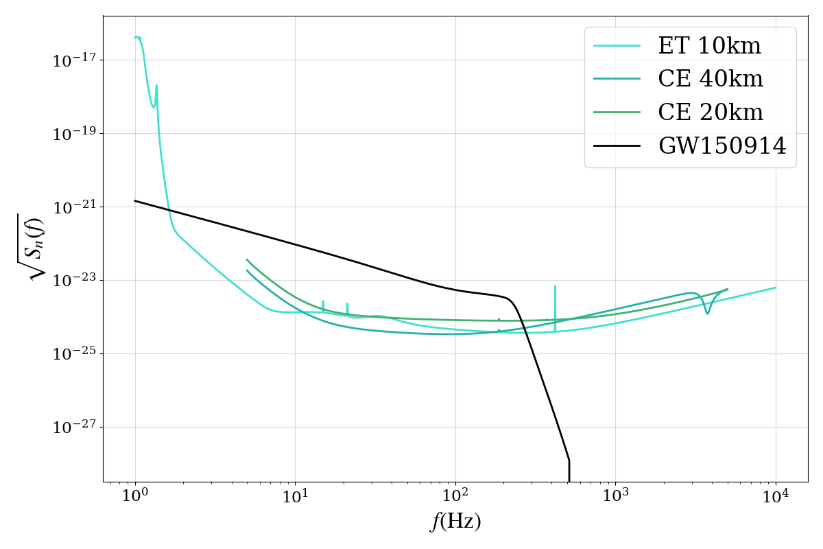
Figure 1: The PSDs of the CE and ET detectors used, plotted with the strain of GW190514-like event with parameters given in the third row (blue row) in Table 1.

One common feature of the three chosen events is that they all have relatively small spins, which makes it hard to put constraints on the spin-dependent finite-size parameters. Therefore we also consider systems with similar masses and redshifts to these, but with artificially amplified spins, i.e. $\chi_{1}=\chi_{2}=0.8$. For these choices of fiducial values, we get much better constraints on the spin-induced quadrupole moment parameter $\kappa_{s}$. However, the price we pay for this choice is that we lose the constraints from the small-spin superradiance condition in Eq. (2.10), which leads to slightly worse constraint on $\mathcal{H}_{0}$ than for small-spin systems.

In Fig. 2, we present the Fisher posterior for a GW150914-like event using the PSDs of CE+ET. This cornerplot showcases the relative degeneracies of the parameters that we are trying to bound as well as their individual variances. We find that the constraints on the finite-size parameters are generally strongly correlated with each other. The direction of the degeneracies in the graph can be mostly understood from the waveform phases given in Eqs. (2.15), (2.16) and (2.17). Heuristically, we can collect the first few relevant finite-size effects:

$$\psi^{\rm FS}\supset\dfrac{3}{128\eta v^{5}}\Bigg{[}-v^{4}\left[50(1-2\eta)\kappa_{s}(\chi_{s}^{2}+\chi_{a}^{2})+\cdots\right]+v^{8}\left[(1-3\log v)\dfrac{25}{2}\mathcal{H}_{0}^{E}+\cdots\right]-v^{10}\left[\dfrac{39}{2}\tilde{\Lambda}\right]\Bigg{]}\leavevmode\nobreak\ .$$ (3.9)

From this expression, we see that the lines of constant phase between 2PN spin-induced moments $\kappa_{s}$ and 5PN Love number $\tilde{\Lambda}$ appear to be negatively correlated. Similar arguments also work for the postive correlation between $\mathcal{H}_{0}^{E}$ and $\tilde{\Lambda}$. The opposite correlations between $\kappa_{s}-\tilde{\Lambda}$ and $\mathcal{H}_{0}-\tilde{\Lambda}$ ensure the Love numbers to be well-constrained.

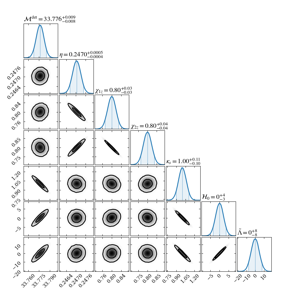
Figure 2: A sample corner plot of the covariance matrix, generated from the Fisher matrix for the GW150914-like event. The center of each graph represents it’s mean (fiducial) value, with the left and right shading bounds representing the $1\sigma$ bound. Here, $\mathcal{M}^{\rm det}$ (in unit of $M_{\odot}$) is the chirp mass in the detector frame.

Finally, we present the marginalized bounds of finite-size parameters $\kappa_{s}$, ${\mathcal{H}}_{0}$ and $\tilde{\Lambda}$ in Table 1. The first line represents the bounds on finite-size effects of GW170817-like event with the fiducial values for Love numbers $\Lambda_{1}=368.2,\Lambda_{2}=586.5$ and dissipation numbers $H_{1\omega}^{E}=0,H_{2\omega}^{E}=0$. Given the relatively small magnitudes of individual spins, we are not able to provide bounds on the spin-induced moments. For tidal dissipations, we choose the fiducial value based on the assumption that neutron stars have almost zero viscosity. In Ref. [62], the authors have shown that for realistic EoS coming from the relativistic mean-field approximation, the 4PN dissipation number purely comes from the contribution of shear viscosity, which scales as $H_{\omega}^{E}\propto T^{-2}$, with $T$ being the neutron star core temperature, so long as the inspiral frequency does not hit the NS gravity mode resonance frequency. For relatively low temperature NSs in a binary system (core temperature $T\sim 10^{5}K$), the dissipation number ranges from $\mathcal{O}(10^{2})$ to $\mathcal{O}(10^{4})$, falling sharply with compactness $H_{\omega}^{E}\propto C^{-6}$, which is defined as $C\equiv GM/R$. Based on the bounds we provide in Table 1, these low-temperature BNS systems may be visible to these forthcoming detectors in the near future.

From the second to the last line in Table 1, we present bounds on finite-size parameters for BBHs. The second and the third lines show the bounds on the GW150914-like event which has relatively high mass. Such an event has a shorter inspiral phase and therefore the constraints are slightly worse than those from the lighter GW151226-like event shown in the fourth and fifth lines. The bounds on dissipation numbers and Love numbers from ET+CE are two order of magnitude better than the bounds we get from the current LVK observations. However, we notice that it is still not possible to rule out the zero dissipaition at the level of individual event which has been claimed for some exotic compact objects [126, 127, 128, 129, 130] . Therefore, to test the nature of BHs, population analysis will be needed. For high spin events, we further put constraints on $\kappa_{s}$. Since this spin-dependent finite-size effects first appear at 2PN order, therefore we get the tightest constraints.

90% bounds for CE+ET Detector Network Results
point-particle parameters					finite-size parameters
$m_{1}$	$m_{2}$	$\chi_{1}$	$\chi_{2}$	$z$	$\tilde{\kappa}$	${\mathcal{H}}_{0}$	$\tilde{\Lambda}$
1.496	1.243	0.00513	0.00323	0.0098	$-$	$0^{+1.8}_{-1.8}$	$456^{+18}_{-18}$
36.2	29.1	0.20	0.20	0.094	$-$	$0.1^{+0.7}_{-0.7}$	$0^{+4.9}_{-4.9}$
36.2	29.1	0.80	0.80	0.094	$1^{+0.23}_{-0.30}$	$0.0^{+0.5}_{-0.7}$	$0^{+15}_{-15}$
14.2	7.5	0.21	0.21	0.090	$-$	$0.2^{+0.3}_{-0.5}$	$0^{+3}_{-3}$
14.2	7.5	0.80	0.80	0.090	$1^{+0.06}_{-0.06}$	$0.0^{+3.3}_{-3.3}$	$0^{+8}_{-8}$

Table 1: Data for parameter bounding for CE+ET network. The first row represents a GW170817-like event, the second/third rows represent a low/high spin GW150914-like event, and the fourth/fifth rows represent a low/high spin GW151226-like event. The third row (blue row) of this table corresponds to the parameters in Fig 2. Note that this table shows the 90% bounds, but the corner plot in Fig. 2 shows the $1\sigma$ bounds for display purpose.

LISA

Likewise, we now present similar marginalized bounds for the same three parameters $\kappa_{s}$, $\mathcal{H}_{0}$, and $\tilde{\Lambda}$ for the LISA detector network in Table 2. The details of calculation remain the same as for the CE+ET network described above. The PSD that we use for LISA analysis is similarly sourced from its respective design review [131].

The GW signals from stellar-mass events fall outside of the parameter space of what LISA is anticipated to be able to observe. Instead, LISA is targeted to detect the GW signals from supermassive BBHs with mass range from $\mathcal{O}(10^{4})$ to $\mathcal{O}(10^{7})$ solar masses. We design four such events, with large ($m_{1}/m_{2}$=9) and small ($m_{1}/m_{2}\approx 1$) mass ratios and large ($\chi_{i}=0.8$) and small ($\chi_{i}=0.2$) spins. The specific data we use and the bounds placed on finite-size parameters thereof are recorded in Table 2. This data shows similar patterns to the CE+ET data, with slightly better bounds overall. The bounds on the spin-induced moments are observed to be comparable with a previous study [84].

90% bounds for LISA Network Results
point particle parameters					finite-size parameters
$m_{1}$	$m_{2}$	$\chi_{1}$	$\chi_{2}$	$z$	$\kappa_{s}$	${\mathcal{H}}_{0}$	$\tilde{\Lambda}$
$5.5\times 10^{5}$	$4.5\times 10^{5}$	0.20	0.20	0.512	$-$	$0.11^{+0.13}_{-0.15}$	$0.0^{+1.3}_{-1.3}$
$5.5\times 10^{5}$	$4.5\times 10^{5}$	0.80	0.80	0.512	$1^{+0.031}_{-0.031}$	$0.1^{+1.3}_{-1.3}$	$0^{+3.3}_{-3.3}$
$9.0\times 10^{5}$	$1.0\times 10^{5}$	0.20	0.20	0.512	$-$	$0.5^{+0.33}_{-0.33}$	$0^{+3}_{-3}$
$9.0\times 10^{5}$	$1.0\times 10^{5}$	0.80	0.80	0.512	$1^{+0.031}_{-0.031}$	$0.4^{+3.1}_{-3.1}$	$0^{+5}_{-5}$

Table 2: Data for parameter bounding for LISA. These point particle parameters are not based on any real data but, mirroring the above table, we sample low- and high-spin components and low- and high-mass-ratio events. We believe this data describes a range of characteristic events that LISA will be able to observe.

4 Conclusions and Outlook

In this paper we have utilized our newly constructed IMRPhenomD+FiniteSize waveform to forecast the constraining power of three future detectors on the $\kappa_{s}$, $\mathcal{H}_{0}$, and $\tilde{\Lambda}$ parameters. Making use of the worldline EFT, we have calculated the finite-size modifications to the point-particle PN framework, and have derived the updated waveform. Using the Fisher matrix method on PSDs for CE, ET, and LISA, we were able to indicate various constraining powers on the finite-size effects for BBHs and BNSs. For CE+ET, we have found bounds for $\kappa_{s}$, $\mathcal{H}_{0}$, and $\tilde{\Lambda}$ of order $\mathcal{O}(10^{-1})$, $\mathcal{O}(10^{0})$, and $\mathcal{O}(10^{1})$, respectively, and we identify that LISA better constrains the values of all of these bounds.

Our work can be extended in various directions that may help get better understanding of the finite-size effects in GW observables. The biggest obstucle we now have is lacking of information about the finite-size contributions to the merger-ringdown part because it is beyond the treatment of worldline EFT. In this paper, we use the taping frequency technique to truncate GW phase evolution due to the finite-size effects before merger and therefore we losing the SNR and further introducing the systematic errors in the waveform modeling. For the future events with high SNR, we need a much more robust and rigorous treatment to have better control on the finite-size effects on the merger-ringdown phase. Secondly, in the analysis for BNSs, we do not put much effort to analyze the magnetic-type finite-size effects. Even though Ref. [39] has pointed out that the magnetic tidal parameters are much smaller compared with corresponding electric ones, it is still interesting to quantify the bounds on these parameters. Additionally, Ref. [132] has shown that the non-linear fluid effects can enhance the GW phase by $10\%\sim 20\%$ at GW frequency 1000 Hz even at Newtonian order. Thus, a complete treatment of non-linear tidal effects seems to be necessary for future detectors.

Appendix A Derivation of IMRPhenomD+FiniteSize Waveform Observables

In this Appendix, we detail the PN derivation of waveform observables including our modifications. In the slow inspiral phase (where the PN expansion is still valid), all of the waveform ovservables including the time-evolution of the frequency and phase are directly governed by the energy balance equation:

$$-\mathcal{F}_{\infty}-\dot{M}=\dot{\mathcal{E}}$$ (A.1)

Where $\mathcal{F}_{\infty}$ is the energy flux at infinity, $\mathcal{E}$ is the binding energy of the system, $M$ is the total mass, and $\dot{X}$ denotes time derivative. Here, $\mathcal{E}$ and $\mathcal{F}_{\infty}$ must both be functions of the object masses, spins, finite-size parameters, and the PN expansion parameter $v=(\pi GMf)^{1/3}$.

The result of the binding energy takes the following form:

$$\mathcal{E}(v)=-\dfrac{M\eta v^{2}}{2}\left(\mathcal{E}_{\rm NS}(v)+\mathcal{E}_{\rm SO}(v)v^{3}+\mathcal{E}_{\rm SS}(v)v^{4}+\mathcal{E}_{\rm SSS}(v)v^{7}+\mathcal{E}_{\rm Love}(v)v^{10}\right)$$ (A.2)

Here $v$ is the expansion velocity. The non-spinning (NS) and spin-orbital (SO) terms are well known and documented in the literature [21, 23, 61]. The spin quadratic (SS) and cubic (SSS) terms contain contributions both from point-particle terms and spin-induced quadrupole moments. Here, we only list the contribution from spin-induced quadrupole moments as

$$\mathcal{E}_{\rm SS}^{\rm SIM}(v) =\chi_{a}\chi_{s}\left(-\dfrac{\delta^{2}\kappa_{a}}{2}-\delta\kappa_{s}-\dfrac{\kappa_{a}}{2}\right)$$

$$+\chi_{s}^{2}\left(-\dfrac{\delta^{2}\kappa_{s}}{4}-\dfrac{\delta\kappa_{a}}{2}-\dfrac{\kappa_{s}}{4}\right)+\chi_{a}^{2}\left(-\dfrac{\delta\kappa_{a}}{2}+\eta\kappa_{s}-\dfrac{\kappa_{s}}{2}\right)$$

$$+v^{2}\Bigg{(}\chi_{a}^{2}\left(\dfrac{25\delta\eta\kappa_{a}}{12}-\dfrac{35\delta\kappa_{a}}{12}-\dfrac{5\eta^{2}\kappa_{s}}{6}+\dfrac{95\eta\kappa_{s}}{12}-\dfrac{35\kappa_{s}}{12}\right)$$

$$+\chi_{a}\chi_{s}\left(\dfrac{25\delta\eta\kappa_{s}}{6}-\dfrac{35\delta\kappa_{s}}{6}-\dfrac{5\eta^{2}\kappa_{a}}{3}+\dfrac{95\eta\kappa_{a}}{6}-\dfrac{35\kappa_{a}}{6}\right)$$

$$+\chi_{s}^{2}\left(\dfrac{25\delta\eta\kappa_{a}}{12}-\dfrac{35\delta\kappa_{a}}{12}-\dfrac{5\eta^{2}\kappa_{s}}{6}+\dfrac{95\eta\kappa_{s}}{12}-\dfrac{35\kappa_{s}}{12}\right)\Bigg{)}$$ (A.3)

$$\mathcal{E}_{\rm SSS}^{\rm SIM}(v) =\chi_{a}\chi_{s}^{2}\left(-2\delta^{2}\eta\kappa_{a}-5\delta^{2}\kappa_{a}+6\delta\eta\kappa_{s}-6\delta\kappa_{s}-\kappa_{a}\right)$$

$$+\chi_{s}^{3}\left(\delta^{3}(-\kappa_{a})-\delta^{2}\eta\kappa_{s}-\dfrac{9\delta^{2}\kappa_{s}}{4}-\delta\kappa_{a}+\dfrac{\kappa_{s}}{4}\right)$$

$$+\chi_{a}^{2}\chi_{s}\left(-6\delta\kappa_{a}+4\eta^{2}\kappa_{s}+12\eta\kappa_{s}-6\kappa_{s}\right)$$

$$+\chi_{a}^{3}(-2\delta\eta\kappa_{s}-2\delta\kappa_{s}+2\eta\kappa_{a}-2\kappa_{a})$$ (A.4)

Similarly, the energy flux at infinity is known to take a similar form:

$$\mathcal{F}_{\infty}=\dfrac{32}{5}\eta^{2}v^{10}\left(\mathcal{F}_{\rm NS}(v)+\mathcal{F}_{\rm SO}(v)v^{3}+\mathcal{F}_{\rm SS}(v)v^{4}+\mathcal{F}_{\rm SSS}(v)v^{7}+\mathcal{F}_{\rm Love}(v)v^{10}\right)$$ (A.5)

where the NS and SO terms are known in the literature [21, 23, 61]. The contributions from the spin-induced quadrupole moments to the energy-flux are

$$\mathcal{F}_{\rm SS}(v) =\chi_{a}\chi_{s}\left(\delta^{2}\kappa_{a}+2\delta\kappa_{s}+\kappa_{a}\right)+\chi_{a}^{2}\left(\delta\kappa_{a}-2\eta\kappa_{s}+\kappa_{s}\right)$$

$$+\chi_{s}^{2}\left(\delta\kappa_{a}-2\eta\kappa_{s}+\kappa_{s}\right)$$

$$+v^{2}\Bigg{(}\chi_{a}^{2}\left(-\dfrac{127\delta\eta\kappa_{a}}{16}+\dfrac{\delta\kappa_{a}}{14}+\dfrac{43\eta^{2}\kappa_{s}}{4}-\dfrac{905\eta\kappa_{s}}{112}+\dfrac{\kappa_{s}}{14}\right)$$

$$+\chi_{a}\chi_{s}\left(-\dfrac{127\delta\eta\kappa_{s}}{8}+\dfrac{\delta\kappa_{s}}{7}+\dfrac{43\eta^{2}\kappa_{a}}{2}-\dfrac{905\eta\kappa_{a}}{56}+\dfrac{\kappa_{a}}{7}\right)$$

$$+\chi_{s}^{2}\left(-\dfrac{127\delta\eta\kappa_{a}}{16}+\dfrac{\delta\kappa_{a}}{14}+\dfrac{43\eta^{2}\kappa_{s}}{4}-\dfrac{905\eta\kappa_{s}}{112}+\dfrac{\kappa_{s}}{14}\right)\Bigg{)}$$

$$+v^{3}\Bigg{(}\chi_{a}^{2}\left(4\pi\delta\kappa_{a}-8\pi\eta\kappa_{s}+4\pi\kappa_{s}\right)+\chi_{a}\chi_{s}\left(8\pi\delta\kappa_{s}-16\pi\eta\kappa_{a}+8\pi\kappa_{a}\right)$$

$$+\chi_{s}^{2}\left(4\pi\delta\kappa_{a}-8\pi\eta\kappa_{s}+4\pi\kappa_{s}\right)\Bigg{)}$$ (A.6)

$$\mathcal{F}_{\rm SSS}(v) =\chi_{a}\chi_{s}^{2}\left(\dfrac{13}{3}\delta^{2}\eta\kappa_{a}+\dfrac{27\delta^{2}\kappa_{a}}{16}+\dfrac{4\delta\eta\kappa_{s}}{3}+\dfrac{15\delta\kappa_{s}}{8}+\dfrac{3\kappa_{a}}{16}\right)$$

$$+\chi_{a}^{2}\chi_{s}\left(\dfrac{95\delta\eta\kappa_{a}}{12}+\dfrac{15\delta\kappa_{a}}{8}-\dfrac{26\eta^{2}\kappa_{s}}{3}+\dfrac{25\eta\kappa_{s}}{6}+\dfrac{15\kappa_{s}}{8}\right)$$

$$+\chi_{s}^{3}\left(-\dfrac{7\delta\eta\kappa_{a}}{4}+\dfrac{5\delta\kappa_{a}}{8}-\dfrac{26\eta^{2}\kappa_{s}}{3}-3\eta\kappa_{s}+\dfrac{5\kappa_{s}}{8}\right)$$

$$+\chi_{a}^{3}\left(\dfrac{29\delta\eta\kappa_{s}}{6}+\dfrac{5\delta\kappa_{s}}{8}+\dfrac{43\eta\kappa_{a}}{12}+\dfrac{5\kappa_{a}}{8}\right)$$ (A.7)

For general tidal dissipation numbers, the horizon flux is given by

$$\dot{M}(v)= \dfrac{1}{2}\left(9\overline{\mathcal{H}}_{1}^{E}\eta^{2}\chi_{a}+9\mathcal{H}_{1}^{E}\eta^{2}\chi_{s}\right)v^{15}+\dfrac{1}{2}\left[\left(9\mathcal{H}_{1}^{B}\eta^{2}+\dfrac{45\mathcal{H}_{1}^{E}\eta^{2}}{2}+\dfrac{9}{2}\overline{\mathcal{H}}_{1}^{E}\delta\eta^{2}-27\mathcal{H}_{1}^{E}\eta^{3}\right)\chi_{s}\right.$$ (A.8)

$$\left.+\left(9\overline{\mathcal{H}}_{1}^{B}\eta^{2}+\dfrac{45\overline{\mathcal{H}}_{1}^{E}\eta^{2}}{2}+\dfrac{9}{2}\mathcal{H}_{1}^{E}\delta\eta^{2}-27\overline{\mathcal{H}}_{1}^{E}\eta^{3}\right)\chi_{a}\right]v^{17}+9\mathcal{H}_{0}\eta^{2}v^{18}$$

where the dissipation numbers $\mathcal{H}_{1}^{E/B},\overline{H}_{1}^{E/B}$ and $\mathcal{H}_{0}$ are defined in Eq. (2.11). The binding energy $\mathcal{E}_{\rm Love}$ and the energy flux $\mathcal{F}_{\rm Love}$ involving Love numbers are given in Ref. [36].

References

- [1] LIGO Scientific, Virgo Collaboration, B. P. Abbott et al., “GWTC-1: A Gravitational-Wave Transient Catalog of Compact Binary Mergers Observed by LIGO and Virgo during the First and Second Observing Runs,” Phys. Rev. X 9 no. 3, (2019) 031040, arXiv:1811.12907 [astro-ph.HE].
- [2] LIGO Scientific, Virgo Collaboration, R. Abbott et al., “GWTC-2: Compact Binary Coalescences Observed by LIGO and Virgo During the First Half of the Third Observing Run,” Phys. Rev. X 11 (2021) 021053, arXiv:2010.14527 [gr-qc].
- [3] LIGO Scientific, VIRGO Collaboration, R. Abbott et al., “GWTC-2.1: Deep Extended Catalog of Compact Binary Coalescences Observed by LIGO and Virgo During the First Half of the Third Observing Run,” arXiv:2108.01045 [gr-qc].
- [4] LIGO Scientific, VIRGO, KAGRA Collaboration, R. Abbott et al., “GWTC-3: Compact Binary Coalescences Observed by LIGO and Virgo During the Second Part of the Third Observing Run,” arXiv:2111.03606 [gr-qc].
- [5] T. Venumadhav, B. Zackay, J. Roulet, L. Dai, and M. Zaldarriaga, “New Search Pipeline for Compact Binary Mergers: Results for Binary Black Holes in the First Observing Run of Advanced LIGO,” Phys. Rev. D100 (2019) 023011, arXiv:1902.10341 [astro-ph.IM].
- [6] T. Venumadhav, B. Zackay, J. Roulet, L. Dai, and M. Zaldarriaga, “New Binary Black Hole Mergers in the Second Observing Run of Advanced LIGO and Advanced Virgo,” Phys. Rev. D 101 (2020) 083030, arXiv:1904.07214 [astro-ph.HE].
- [7] S. Olsen, T. Venumadhav, J. Mushkin, J. Roulet, B. Zackay, and M. Zaldarriaga, “New binary black hole mergers in the LIGO-Virgo O3a data,” Phys. Rev. D 106 no. 4, (2022) 043009, arXiv:2201.02252 [astro-ph.HE].
- [8] A. H. Nitz, C. Capano, A. B. Nielsen, S. Reyes, R. White, D. A. Brown, and B. Krishnan, “1-OGC: The first open gravitational-wave catalog of binary mergers from analysis of public Advanced LIGO data,” Astrophys. J. 872 no. 2, (2019) 195, arXiv:1811.01921 [gr-qc].
- [9] A. H. Nitz, T. Dent, G. S. Davies, S. Kumar, C. D. Capano, I. Harry, S. Mozzon, L. Nuttall, A. Lundgren, and M. Tápai, “2-OGC: Open Gravitational-wave Catalog of Binary Mergers from Analysis of Public Advanced LIGO and Virgo Data,” Astrophys. J. 891 (10, 2019) 123, arXiv:1910.05331 [astro-ph.HE].
- [10] A. H. Nitz, C. D. Capano, S. Kumar, Y.-F. Wang, S. Kastha, M. Schäfer, R. Dhurkunde, and M. Cabero, “3-OGC: Catalog of Gravitational Waves from Compact-binary Mergers,” Astrophys. J. 922 no. 1, (2021) 76, arXiv:2105.09151 [astro-ph.HE].
- [11] A. H. Nitz, S. Kumar, Y.-F. Wang, S. Kastha, S. Wu, M. Schäfer, R. Dhurkunde, and C. D. Capano, “4-OGC: Catalog of Gravitational Waves from Compact Binary Mergers,” Astrophys. J. 946 no. 2, (2023) 59, arXiv:2112.06878 [astro-ph.HE].
- [12] H. S. Chia, T. D. P. Edwards, D. Wadekar, A. Zimmerman, S. Olsen, J. Roulet, T. Venumadhav, B. Zackay, and M. Zaldarriaga, “In Pursuit of Love: First Templated Search for Compact Objects with Large Tidal Deformabilities in the LIGO-Virgo Data,” arXiv:2306.00050 [gr-qc].
- [13] A. K. Mehta, S. Olsen, D. Wadekar, J. Roulet, T. Venumadhav, J. Mushkin, B. Zackay, and M. Zaldarriaga, “New binary black hole mergers in the LIGO-Virgo O3b data,” arXiv:2311.06061 [gr-qc].
- [14] D. Wadekar, J. Roulet, T. Venumadhav, A. K. Mehta, B. Zackay, J. Mushkin, S. Olsen, and M. Zaldarriaga, “New black hole mergers in the LIGO-Virgo O3 data from a gravitational wave search including higher-order harmonics,” arXiv:2312.06631 [gr-qc].
- [15] L. Blanchet, “Gravitational Radiation from Post-Newtonian Sources and Inspiralling Compact Binaries,” Living Rev. Rel. 17 (2014) 2, arXiv:1310.1528 [gr-qc].
- [16] J. Blümlein, A. Maier, P. Marquard, and G. Schäfer, “The fifth-order post-Newtonian Hamiltonian dynamics of two-body systems from an effective field theory approach,” Nucl. Phys. B 983 (2022) 115900, arXiv:2110.13822 [gr-qc]. [Erratum: Nucl.Phys.B 985, 115991 (2022)].
- [17] J. Blümlein, A. Maier, P. Marquard, and G. Schäfer, “The 6th post-Newtonian potential terms at ,” Phys. Lett. B 816 (2021) 136260, arXiv:2101.08630 [gr-qc].
- [18] G. Cho, R. A. Porto, and Z. Yang, “Gravitational radiation from inspiralling compact objects: Spin effects to the fourth post-Newtonian order,” Phys. Rev. D 106 no. 10, (2022) L101501, arXiv:2201.05138 [gr-qc].
- [19] L. Blanchet, G. Faye, Q. Henry, F. Larrouturou, and D. Trestini, “Gravitational waves from compact binaries to the fourth post-Newtonian order,” in 57th Rencontres de Moriond on Gravitation. 4, 2023. arXiv:2304.13647 [gr-qc].
- [20] D. Trestini and L. Blanchet, “Gravitational-wave tails of memory at 4PN order,” in 57th Rencontres de Moriond on Gravitation. 6, 2023. arXiv:2306.00546 [gr-qc].
- [21] L. Blanchet, G. Faye, and D. Trestini, “Gravitational radiation reaction for compact binary systems at the fourth-and-a-half post-Newtonian order,” arXiv:2407.18295 [gr-qc].
- [22] E. Poisson and C. Will, Gravity: Newtonian, Post-Newtonian, Relativistic. Cambridge University Press, 2014. https://books.google.com/books?id=PZ5cAwAAQBAJ.
- [23] L. Blanchet, “Post-Newtonian theory for gravitational waves,” Living Rev. Rel. 27 no. 1, (2024) 4.
- [24] E. Poisson, “Gravitational Waves from Inspiraling Compact Binaries: The Quadrupole Moment Term,” Phys. Rev. D 57 (1998) 5287, arXiv:gr-qc/9709032 [gr-qc].
- [25] R. A. Porto, “Post-Newtonian corrections to the motion of spinning bodies in NRGR,” Phys. Rev. D 73 (2006) 104031, arXiv:gr-qc/0511061.
- [26] S. Marsat, “Cubic Order Spin Effects in the Dynamics and Gravitational Wave Energy Flux of Compact Object Binaries,” Class. Quant. Grav. 32 (2015) 085008, arXiv:1411.4118 [gr-qc].
- [27] M. Levi and J. Steinhoff, “Leading Order Finite Size Effects with Spins for Inspiralling Compact Binaries,” JHEP 06 (2015) 059, arXiv:1410.2601 [gr-qc].
- [28] M. Levi and J. Steinhoff, “Spinning gravitating objects in the effective field theory in the post-Newtonian scheme,” JHEP 09 (2015) 219, arXiv:1501.04956 [gr-qc].
- [29] N. Krishnendu, K. Arun, and C. Mishra, “Testing the Binary Black Hole Nature of a Compact Binary Coalescence,” Phys. Rev. Lett. 119 (2017) 091101, arXiv:1701.06318 [gr-qc].
- [30] N. V. Krishnendu, C. K. Mishra, and K. G. Arun, “Spin-Induced Deformations and Tests of Binary Black Hole Nature Using Third-Generation Detectors,” Phys. Rev. D99 (2019) 064008, arXiv:1811.00317 [gr-qc].
- [31] H. S. Chia and T. D. Edwards, “Searching for General Binary Inspirals with Gravitational Waves,” JCAP 11 (2020) 033, arXiv:2004.06729 [astro-ph.HE].
- [32] H. S. Chia, T. D. P. Edwards, R. N. George, A. Zimmerman, A. Coogan, K. Freese, C. Messick, and C. N. Setzer, “Dimensionally Reduced Waveforms for Spin-Induced Quadrupole Searches,” arXiv:2211.00039 [gr-qc].
- [33] Z. Lyu, M. LaHaye, H. Yang, and B. Bonga, “Probing spin-induced quadrupole moments in precessing compact binaries,” Phys. Rev. D 109 no. 6, (2024) 064081, arXiv:2308.09032 [gr-qc].
- [34] H. Love, “Some problems of geodynamics,” Nature 89 no. 2228, (1912) 471–472. https://doi.org/10.1038/089471a0.
- [35] W. D. Goldberger and I. Z. Rothstein, “An Effective field theory of gravity for extended objects,” Phys. Rev. D 73 (2006) 104029, arXiv:hep-th/0409156.
- [36] E. Flanagan and T. Hinderer, “Constraining Neutron Star Tidal Love Numbers with Gravitational Wave Detectors,” Phys. Rev. D 77 (2008) 021502, arXiv:0709.1915 [astro-ph].
- [37] C. Li and G. Lovelace, “A Generalization of Ryan’s theorem: Probing tidal coupling with gravitational waves from nearly circular, nearly equatorial, extreme-mass-ratio inspirals,” Phys. Rev. D 77 (2008) 064022, arXiv:gr-qc/0702146.
- [38] T. Damour and A. Nagar, “Relativistic Tidal Properties of Neutron Stars,” Phys. Rev. D 80 (2009) 084035, arXiv:0906.0096 [gr-qc].
- [39] T. Binnington and E. Poisson, “Relativistic Theory of Tidal Love Numbers,” Phys. Rev. D 80 (2009) 084018, arXiv:0906.1366 [gr-qc].
- [40] J. Vines, E. E. Flanagan, and T. Hinderer, “Post-1-Newtonian Tidal Effects in the Gravitational Waveform from Binary Inspirals,” Phys. Rev. D 83 (2011) 084051, arXiv:1101.1673 [gr-qc].
- [41] V. Cardoso, E. Franzin, A. Maselli, P. Pani, and G. Raposo, “Testing Strong-Field Gravity with Tidal Love Numbers,” Phys. Rev. D 95 (2017) 084014, arXiv:1701.01116 [gr-qc]. [Addendum: Phys. Rev. D 95 (2017) 089901].
- [42] J. B. Hartle, “Tidal friction in slowly rotating black holes,” Phys. Rev. D 8 (Aug, 1973) 1010–1024. https://link.aps.org/doi/10.1103/PhysRevD.8.1010.
- [43] E. Poisson and M. Sasaki, “Gravitational radiation from a particle in circular orbit around a black hole. 5: Black hole absorption and tail corrections,” Phys. Rev. D 51 (1995) 5753–5767, arXiv:gr-qc/9412027.
- [44] H. Tagoshi, S. Mano, and E. Takasugi, “PostNewtonian expansion of gravitational waves from a particle in circular orbits around a rotating black hole: Effects of black hole absorption,” Prog. Theor. Phys. 98 (1997) 829–850, arXiv:gr-qc/9711072.
- [45] K. Alvi, “Energy and angular momentum flow into a black hole in a binary,” Phys. Rev. D 64 (2001) 104020, arXiv:gr-qc/0107080.
- [46] S. A. Hughes, “Evolution of circular, nonequatorial orbits of Kerr black holes due to gravitational wave emission. II. Inspiral trajectories and gravitational wave forms,” Phys. Rev. D 64 (2001) 064004, arXiv:gr-qc/0104041. [Erratum: Phys.Rev.D 88, 109902 (2013)].
- [47] E. Poisson, “Tidal interaction of black holes and Newtonian viscous bodies,” Phys. Rev. D 80 (2009) 064029, arXiv:0907.0874 [gr-qc].
- [48] J.-P. Zahn, “Tidal dissipation in binary systems,” EAS Publ. Ser. 29 (2008) 67, arXiv:0807.4870 [astro-ph].
- [49] G. I. Ogilvie, “Tidal dissipation in stars and giant planets,” Ann. Rev. Astron. Astrophys. 52 (2014) 171–210, arXiv:1406.2207 [astro-ph.SR].
- [50] E. Poisson and C. M. Will, Gravity: Newtonian, Post-Newtonian, Relativistic. Cambridge University Press, 2014.
- [51] C. D. Murray and S. F. Dermott, Solar system dynamics. Cambridge university press, 1999.
- [52] M. Punturo et al., “The Einstein Telescope: A third-generation gravitational wave observatory,” Class. Quant. Grav. 27 (2010) 194002.
- [53] S. Hild et al., “Sensitivity Studies for Third-Generation Gravitational Wave Observatories,” Class. Quant. Grav. 28 (2011) 094013, arXiv:1012.0908 [gr-qc].
- [54] D. Reitze et al., “Cosmic Explorer: The U.S. Contribution to Gravitational-Wave Astronomy Beyond LIGO,” Bull. Am. Astron. Soc. 51 (7, 2019) 035, arXiv:1907.04833 [astro-ph.IM].
- [55] M. Evans et al., “A Horizon Study for Cosmic Explorer: Science, Observatories, and Community,” arXiv:2109.09882 [astro-ph.IM].
- [56] P. Amaro-Seoane, H. Audley, et al., “Laser interferometer space antenna,” arXiv preprint arXiv:1702.00786 (2017) .
- [57] R. Hansen, “Multipole Moments of Stationary Spacetimes,” J. Math. Phys. 15 (1974) 46.
- [58] K. Thorne, “Multipole Expansions of Gravitational Radiation,” Rev. Mod. Phys. 52 (1980) 299–339.
- [59] M. V. S. Saketh, J. Steinhoff, J. Vines, and A. Buonanno, “Modeling horizon absorption in spinning binary black holes using effective worldline theory,” arXiv:2212.13095 [gr-qc].
- [60] M. V. S. Saketh, Z. Zhou, and M. M. Ivanov, “Dynamical Tidal Response of Kerr Black Holes from Scattering Amplitudes,” arXiv:2307.10391 [hep-th].
- [61] H. S. Chia, Z. Zhou, and M. M. Ivanov, “Bring the Heat: Tidal Heating Constraints for Black Holes and Exotic Compact Objects from the LIGO-Virgo-KAGRA Data,” arXiv:2404.14641 [gr-qc].
- [62] M. V. S. Saketh, Z. Zhou, S. Ghosh, J. Steinhoff, and D. Chatterjee, “Investigating tidal heating in neutron stars via gravitational Raman scattering,” arXiv:2407.08327 [gr-qc].
- [63] S. Endlich and R. Penco, “Effective field theory approach to tidal dynamics of spinning astrophysical systems,” Phys. Rev. D 93 no. 6, (2016) 064021, arXiv:1510.08889 [gr-qc].
- [64] B. Kol and M. Smolkin, “Black Hole Stereotyping: Induced Gravito-Static Polarization,” JHEP 02 (2012) 010, arXiv:1110.3764 [hep-th].
- [65] L. Hui, A. Joyce, R. Penco, L. Santoni, and A. R. Solomon, “Static response and Love numbers of Schwarzschild black holes,” JCAP 04 (2021) 052, arXiv:2010.00593 [hep-th].
- [66] A. Le Tiec and M. Casals, “Spinning Black Holes Fall in Love,” Phys. Rev. Lett. 126 no. 13, (2021) 131102, arXiv:2007.00214 [gr-qc].
- [67] H. S. Chia, “Tidal deformation and dissipation of rotating black holes,” Phys. Rev. D 104 no. 2, (2021) 024013, arXiv:2010.07300 [gr-qc].
- [68] P. Charalambous, S. Dubovsky, and M. M. Ivanov, “On the Vanishing of Love Numbers for Kerr Black Holes,” JHEP 05 (2021) 038, arXiv:2102.08917 [hep-th].
- [69] P. Charalambous, S. Dubovsky, and M. M. Ivanov, “Hidden Symmetry of Vanishing Love Numbers,” Phys. Rev. Lett. 127 no. 10, (2021) 101101, arXiv:2103.01234 [hep-th].
- [70] L. Hui, A. Joyce, R. Penco, L. Santoni, and A. R. Solomon, “Ladder symmetries of black holes. Implications for love numbers and no-hair theorems,” JCAP 01 no. 01, (2022) 032, arXiv:2105.01069 [hep-th].
- [71] P. Charalambous, S. Dubovsky, and M. M. Ivanov, “Love symmetry,” JHEP 10 (2022) 175, arXiv:2209.02091 [hep-th].
- [72] M. M. Ivanov and Z. Zhou, “Vanishing of Black Hole Tidal Love Numbers from Scattering Amplitudes,” Phys. Rev. Lett. 130 no. 9, (2023) 091403, arXiv:2209.14324 [hep-th].
- [73] L. Hui, A. Joyce, R. Penco, L. Santoni, and A. R. Solomon, “Near-zone symmetries of Kerr black holes,” JHEP 09 (2022) 049, arXiv:2203.08832 [hep-th].
- [74] V. De Luca, J. Khoury, and S. S. C. Wong, “Implications of the weak gravity conjecture for tidal Love numbers of black holes,” Phys. Rev. D 108 no. 4, (2023) 044066, arXiv:2211.14325 [hep-th].
- [75] P. Charalambous and M. M. Ivanov, “Scalar Love numbers and Love symmetries of 5-dimensional Myers-Perry black holes,” JHEP 07 (2023) 222, arXiv:2303.16036 [hep-th].
- [76] M. J. Rodriguez, L. Santoni, A. R. Solomon, and L. F. Temoche, “Love numbers for rotating black holes in higher dimensions,” Phys. Rev. D 108 no. 8, (2023) 084011, arXiv:2304.03743 [hep-th].
- [77] V. De Luca, J. Khoury, and S. S. C. Wong, “Nonlinearities in the tidal Love numbers of black holes,” Phys. Rev. D 108 no. 2, (2023) 024048, arXiv:2305.14444 [gr-qc].
- [78] P. Charalambous, “Love numbers and Love symmetries for -form and gravitational perturbations of higher-dimensional spherically symmetric black holes,” arXiv:2402.07574 [hep-th].
- [79] E. Berti, V. De Luca, L. Del Grosso, and P. Pani, “Tidal Love numbers and approximate universal relations for fermion soliton stars,” arXiv:2404.06979 [gr-qc].
- [80] T. Hinderer, “Tidal Love Numbers of Neutron Stars,” Astrophys. J. 677 (2008) 1216, arXiv:0711.2420 [astro-ph].
- [81] LIGO Scientific, Virgo Collaboration, B. P. Abbott et al., “GW170817: Observation of Gravitational Waves from a Binary Neutron Star Inspiral,” Phys. Rev. Lett. 119 no. 16, (2017) 161101, arXiv:1710.05832 [gr-qc].
- [82] LIGO Scientific, Virgo Collaboration, B. P. Abbott et al., “Properties of the binary neutron star merger GW170817,” Phys. Rev. X 9 no. 1, (2019) 011001, arXiv:1805.11579 [gr-qc].
- [83] S. Kastha, A. Gupta, K. G. Arun, B. S. Sathyaprakash, and C. Van Den Broeck, “Testing the Multipole Structure of Compact Binaries Using Gravitational Save Observations,” Phys. Rev. D98 (2018) 124033, arXiv:1809.10465 [gr-qc].
- [84] N. V. Krishnendu and A. B. Yelikar, “Testing the Kerr nature of supermassive and intermediate-mass black hole binaries using spin-induced multipole moment measurements,” Class. Quant. Grav. 37 no. 20, (2020) 205019, arXiv:1904.12712 [gr-qc].
- [85] N. V. Krishnendu, M. Saleem, A. Samajdar, K. G. Arun, W. Del Pozzo, and C. K. Mishra, “Constraints on the binary black hole nature of GW151226 and GW170608 from the measurement of spin-induced quadrupole moments,” Phys. Rev. D 100 no. 10, (2019) 104019, arXiv:1908.02247 [gr-qc].
- [86] T. Narikawa, N. Uchikata, and T. Tanaka, “Gravitational-wave constraints on the GWTC-2 events by measuring the tidal deformability and the spin-induced quadrupole moment,” Phys. Rev. D 104 no. 8, (2021) 084056, arXiv:2106.09193 [gr-qc].
- [87] M. Saleem, N. V. Krishnendu, A. Ghosh, A. Gupta, W. Del Pozzo, A. Ghosh, and K. G. Arun, “Population inference of spin-induced quadrupole moments as a probe for nonblack hole compact binaries,” Phys. Rev. D 105 no. 10, (2022) 104066, arXiv:2111.04135 [gr-qc].
- [88] J. L. Ripley, A. Hegade K. R., R. S. Chandramouli, and N. Yunes, “First constraint on the dissipative tidal deformability of neutron stars,” arXiv:2312.11659 [gr-qc].
- [89] A. Hegade K. R., J. L. Ripley, and N. Yunes, “Dissipative tidal effects to next-to-leading order and constraints on the dissipative tidal deformability using gravitational wave data,” Phys. Rev. D 110 no. 4, (2024) 044041, arXiv:2407.02584 [gr-qc].
- [90] W. Laarakkers and E. Poisson, “Quadrupole Moments of Rotating Neutron Stars,” Astrophys. J. 512 (1999) 282, arXiv:gr-qc/9709033 [gr-qc].
- [91] G. Pappas and T. Apostolatos, “Revising the Multipole Moments of Numerical Spacetimes, and its Consequences,” Phys. Rev. Lett. 108 (2012) 231104, arXiv:1201.6067 [gr-qc].
- [92] A. Hegade K. R., J. L. Ripley, and N. Yunes, “Dynamical tidal response of non-rotating relativistic stars,” arXiv:2403.03254 [gr-qc].
- [93] V. Srivastava, D. Davis, K. Kuns, P. Landry, S. Ballmer, M. Evans, E. D. Hall, J. Read, and B. S. Sathyaprakash, “Science-driven Tunable Design of Cosmic Explorer Detectors,” Astrophys. J. 931 no. 1, (2022) 22, arXiv:2201.10668 [gr-qc].
- [94] M. Branchesi et al., “Science with the Einstein Telescope: a comparison of different designs,” JCAP 07 (2023) 068, arXiv:2303.15923 [gr-qc].
- [95] P. Dutta Roy, S. Datta, and K. G. Arun, “Tests of general relativity at the fourth post-Newtonian order,” Phys. Rev. D 110 no. 6, (2024) 064002, arXiv:2406.07691 [gr-qc].
- [96] M. Tse et al., “Quantum-Enhanced Advanced LIGO Detectors in the Era of Gravitational-Wave Astronomy,” Phys. Rev. Lett. 123 no. 23, (2019) 231107.
- [97] VIRGO Collaboration, F. Acernese et al., “Advanced Virgo: a second-generation interferometric gravitational wave detector,” Class. Quant. Grav. 32 no. 2, (2015) 024001, arXiv:1408.3978 [gr-qc].
- [98] C. Unnikrishnan, “IndIGO and LIGO-India: Scope and Plans for Gravitational Wave Research and Precision Metrology in India,” Int. J. Mod. Phys. D 22 (2013) 1341010, arXiv:1510.06059 [physics.ins-det].
- [99] M. Saleem et al., “The science case for LIGO-India,” Class. Quant. Grav. 39 no. 2, (2022) 025004, arXiv:2105.01716 [gr-qc].
- [100] W. D. Goldberger and I. Z. Rothstein, “Dissipative effects in the worldline approach to black hole dynamics,” Phys. Rev. D 73 (2006) 104030, arXiv:hep-th/0511133.
- [101] W. D. Goldberger and A. Ross, “Gravitational radiative corrections from effective field theory,” Phys. Rev. D 81 (2010) 124015, arXiv:0912.4254 [gr-qc].
- [102] R. A. Porto, “The effective field theorist’s approach to gravitational dynamics,” Phys. Rept. 633 (2016) 1–104, arXiv:1601.04914 [hep-th].
- [103] M. Levi, “Effective Field Theories of Post-Newtonian Gravity: A comprehensive review,” Rept. Prog. Phys. 83 no. 7, (2020) 075901, arXiv:1807.01699 [hep-th].
- [104] W. D. Goldberger, J. Li, and I. Z. Rothstein, “Non-conservative effects on spinning black holes from world-line effective field theory,” JHEP 06 (2021) 053, arXiv:2012.14869 [hep-th].
- [105] J. Steinhoff, T. Hinderer, T. Dietrich, and F. Foucart, “Spin effects on neutron star fundamental-mode dynamical tides: Phenomenology and comparison to numerical simulations,” Phys. Rev. Res. 3 no. 3, (2021) 033129, arXiv:2103.06100 [gr-qc].
- [106] C. Pacilio, A. Maselli, M. Fasano, and P. Pani, “Ranking Love Numbers for the Neutron Star Equation of State: The Need for Third-Generation Detectors,” Phys. Rev. Lett. 128 no. 10, (2022) 101101, arXiv:2104.10035 [gr-qc].
- [107] F. Iacovelli, M. Mancarella, C. Mondal, A. Puecher, T. Dietrich, F. Gulminelli, M. Maggiore, and M. Oertel, “Nuclear physics constraints from binary neutron star mergers in the Einstein Telescope era,” Phys. Rev. D 108 no. 12, (2023) 122006, arXiv:2308.12378 [gr-qc].
- [108] R. Huxford, R. Kashyap, S. Borhanian, A. Dhani, I. Gupta, and B. S. Sathyaprakash, “Accuracy of neutron star radius measurement with the next generation of terrestrial gravitational-wave observatories,” Phys. Rev. D 109 no. 10, (2024) 103035, arXiv:2307.05376 [gr-qc].
- [109] S. A. Teukolsky, “Perturbations of a rotating black hole. i. fundamental equations for gravitational, electromagnetic, and neutrino-field perturbations,” The Astrophysical Journal 185 (1973) 635–648.
- [110] S. A. Teukolsky and W. Press, “Perturbations of a rotating black hole. iii-interaction of the hole with gravitational and electromagnetic radiation,” The Astrophysical Journal 193 (1974) 443–461.
- [111] S. Chandrasekhar, The mathematical theory of black holes. 1985.
- [112] R. A. Porto, “Absorption effects due to spin in the worldline approach to black hole dynamics,” Phys. Rev. D 77 (2008) 064026, arXiv:0710.5150 [hep-th].
- [113] W. D. Goldberger, “Effective field theories of gravity and compact binary dynamics: A Snowmass 2021 whitepaper,” in 2022 Snowmass Summer Study. 6, 2022. arXiv:2206.14249 [hep-th].
- [114] W. D. Goldberger, “Effective Field Theory for Compact Binary Dynamics,” arXiv:2212.06677 [hep-th].
- [115] R. A. Porto and I. Z. Rothstein, “Spin(1)Spin(2) Effects in the Motion of Inspiralling Compact Binaries at Third Order in the Post-Newtonian Expansion,” Phys. Rev. D 78 (2008) 044012, arXiv:0802.0720 [gr-qc]. [Erratum: Phys.Rev.D 81, 029904 (2010)].
- [116] P. Saini and N. V. Krishnendu, “Constraining the nature of dark compact objects with spin-induced octupole moment measurement,” Phys. Rev. D 109 no. 2, (2024) 024009, arXiv:2308.01309 [gr-qc].
- [117] K. Thorne, “Gravitational Radiation,” in 300 Years of Gravitation, S. Hawking and W. Israel, eds., pp. 330. Cambridge University Press. 1987.
- [118] A. K. Mehta, A. Buonanno, R. Cotesta, A. Ghosh, N. Sennett, and J. Steinhoff, “Tests of general relativity with gravitational-wave observations using a flexible theory-independent method,” Phys. Rev. D 107 no. 4, (2023) 044020, arXiv:2203.13937 [gr-qc].
- [119] C. Cutler and E. E. Flanagan, “Gravitational waves from merging compact binaries: How accurately can one extract the binary’s parameters from the inspiral waveform?” Phys. Rev. D 49 (Mar, 1994) 2658–2697. https://link.aps.org/doi/10.1103/PhysRevD.49.2658.
- [120] M. Vallisneri, “Use and abuse of the Fisher information matrix in the assessment of gravitational-wave parameter-estimation prospects,” Phys. Rev. D 77 (2008) 042001, arXiv:gr-qc/0703086.
- [121] C. L. Rodriguez, B. Farr, W. M. Farr, and I. Mandel, “Inadequacies of the Fisher Information Matrix in gravitational-wave parameter estimation,” Phys. Rev. D 88 no. 8, (2013) 084013, arXiv:1308.1397 [astro-ph.IM].
- [122] F. Iacovelli, M. Mancarella, S. Foffa, and M. Maggiore, “Forecasting the Detection Capabilities of Third-generation Gravitational-wave Detectors Using GWFAST,” Astrophys. J. 941 no. 2, (2022) 208, arXiv:2207.02771 [gr-qc].
- [123] M. Maggiore, Gravitational Waves. Vol. 1: Theory and Experiments. Oxford University Press, 2007.
- [124] LIGO Scientific, Virgo Collaboration, B. P. Abbott et al., “Observation of Gravitational Waves from a Binary Black Hole Merger,” Phys. Rev. Lett. 116 no. 6, (2016) 061102, arXiv:1602.03837 [gr-qc].
- [125] LIGO Scientific, Virgo Collaboration, B. P. Abbott et al., “GW151226: Observation of Gravitational Waves from a 22-Solar-Mass Binary Black Hole Coalescence,” Phys. Rev. Lett. 116 no. 24, (2016) 241103, arXiv:1606.04855 [gr-qc].
- [126] A. Maselli, P. Pani, V. Cardoso, T. Abdelsalhin, L. Gualtieri, and V. Ferrari, “Probing Planckian Corrections at the Horizon Scale with LISA Binaries,” Phys. Rev. Lett. 120 (2018) 081101, arXiv:1703.10612 [gr-qc].
- [127] S. Datta and S. Bose, “Probing the nature of central objects in extreme-mass-ratio inspirals with gravitational waves,” Phys. Rev. D 99 no. 8, (2019) 084001, arXiv:1902.01723 [gr-qc].
- [128] S. Datta, R. Brito, S. Bose, P. Pani, and S. A. Hughes, “Tidal heating as a discriminator for horizons in extreme mass ratio inspirals,” Phys. Rev. D 101 no. 4, (2020) 044004, arXiv:1910.07841 [gr-qc].
- [129] S. Datta, R. Brito, S. A. Hughes, T. Klinger, and P. Pani, “Tidal heating as a discriminator for horizons in equatorial eccentric extreme mass ratio inspirals,” arXiv:2404.04013 [gr-qc].
- [130] S. Mukherjee, S. Datta, S. Tiwari, K. S. Phukon, and S. Bose, “Toward establishing the presence or absence of horizons in coalescing binaries of compact objects by using their gravitational wave signals,” Phys. Rev. D 106 no. 10, (2022) 104032, arXiv:2202.08661 [gr-qc].
- [131] T. Robson, N. J. Cornish, and C. Liu, “The construction and use of LISA sensitivity curves,” Class. Quant. Grav. 36 no. 10, (2019) 105011, arXiv:1803.01944 [astro-ph.HE].
- [132] H. Yu, N. N. Weinberg, P. Arras, J. Kwon, and T. Venumadhav, “Beyond the linear tide: impact of the non-linear tidal response of neutron stars on gravitational waveforms from binary inspirals,” Mon. Not. Roy. Astron. Soc. 519 no. 3, (2023) 4325–4343, arXiv:2211.07002 [gr-qc].
- [133] F. Iacovelli, M. Mancarella, S. Foffa, and M. Maggiore, “GWFAST: A Fisher Information Matrix Python Code for Third-generation Gravitational-wave Detectors,” Astrophys. J. Supp. 263 no. 1, (2022) 2, arXiv:2207.06910 [astro-ph.IM].