Embodied Visuomotor Representation

Suppose you are at your desk looking at some objects on it. You don’t know the precise distance from your eye to any particular object in meters. However, you can immediately reach out and touch any of them. Instead of the meter, your knowledge of distance is encoded in unknown but embodied units of action. In contrast, standard approaches in robotics assume calibration to the meter, so that separated vision and control processes can be interfaced. Consequently, robots are precisely manufactured and calibrated, resulting in expensive systems available in only a few configurations.

In response, we propose Embodied Visuomotor Representation, a framework that allows distance to be measured by a robot’s own actions and thus minimizes dependence on calibrated 3D sensors and physical models. Using it, we demonstrate that a robot without knowledge of its size, environmental scale, or its own strength can become capable of touching and clearing obstacles after several seconds of operation. Similarly, we demonstrate in simulation that an agent, without knowledge of its mass or strength, can jump a gap of unknown size after performing a few test oscillations. These experiments parallel bee and gerbil behavior, respectively.

The prevailing autonomy frameworks in robotics rely on calibrated 3D sensors, pre-determined models of their physical form, and structured representations of environmental interactions. This allows vision and low-level control to be abstracted by the implicit assumption of an external scale, such as the meter, to coordinate them. For example, it is common to construct a passive visual process that estimates distances and builds a metric map scaled to the meter. Next, the geometry of the world is used by a planning algorithm to design a trajectory scaled to the meter. Then a pre-tuned low-level controller uses feedback to follow the metric trajectory by mapping it to motor signals. This is called the sense, plan, act paradigm, and it has its roots in the Marr paradigm of vision  (?). Figure 1 shows a block diagram of the sense-plan-act paradigm.

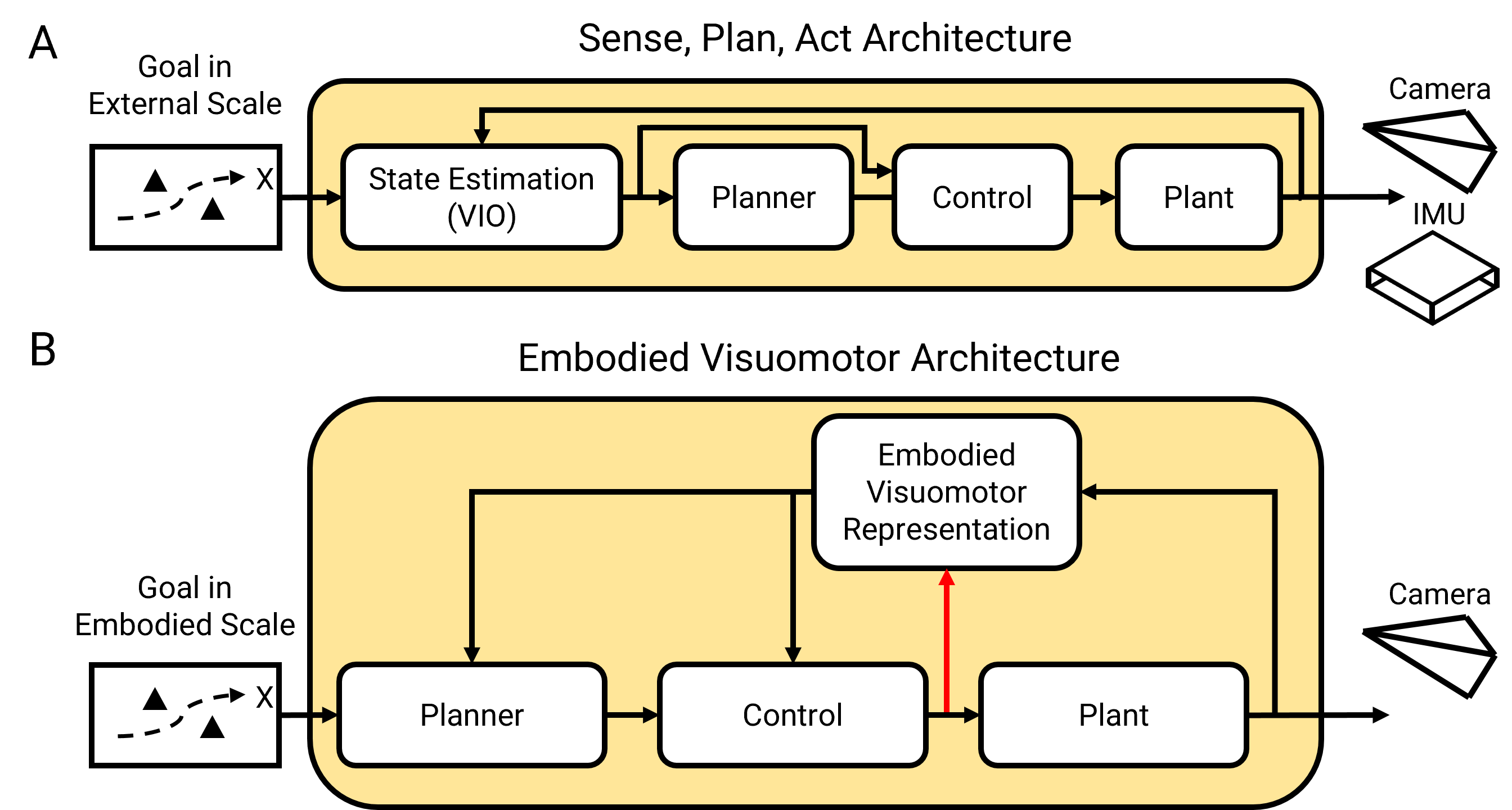
Figure 1: (A): The classic sense-plan-act architecture used in robotics assuming VIO is used for state estimation. (B): An architecture based on Embodied Visuomotor Representation. Compared to sense-plan-act, the embodied approach includes an additional internal feedback connection (red arrow), that allows it to develop an embodied sense of scale without access to calibrated sensors such as an IMU. The resulting measurements naturally result in stable closed-loop control. On the other hand, the sense-plan-act loop’s stability depends on accurate calibration of the sensors to an external scale.

The sense-plan-act architecture allows largely separate teams of engineers and scientists to create equally separate vision and control algorithms tuned for particular tasks and mechanical configurations. Subsequently, alternative frameworks for vision such as Active Vision and Animate Vision emerged  (?, ?, ?) primarily to address the limitations of the passive role of vision in the sense-plan-act cycle. However these frameworks consider control (action) at a high level, and so vision and control remain mostly separate fields and continued to be interfaced with external scale. This dependence leads to lengthy design-build-test cycles and, consequently, expensive systems that are available in only a few physical configurations and must be precisely manufactured. Further, it creates problems that are unobserved in biological systems. For example, it is well-known that Advanced Driver-Assistance Systems (ADAS) in modern cars, such as lane-keeping assist and collision warning, require millimeter accurate, per vehicle calibrations. Another example is the 1999 NASA Mars Climate Orbiter, whose software confused English and Metric units and crashed  (?). Finally, there are several billion dollar 3D Camera and LIDAR industries, whose purpose is to produce accurate 3D measurements calibrated to an external scale, and significant effort is dedicated to ensuring those calibrations do not degrade over time. Meanwhile, non-autonomous drones, cars, and walking robots are cheap enough to be popular toys and humans can easily learn to control them without the benefit of calibration to external scale. Further, we know from psychology that human and other mammalian perceptual systems do not provide metric depth and shape  (?, ?, ?, ?, ?).

This situation is striking because biological systems do not necessarily have access to an external scale like the meter. Instead, somehow they must represent the world using only the embodied signals due to their physical form. Regardless, animals such as humans, dragonflies, and bumblebees exhibit visuomotor capabilities far in excess of robots while also allowing for much wider variation in physical form and more complex dynamics, such as turbulence and muscular response  (?, ?, ?). Thus, we call methods that capture these phenomena embodied visuomotor representation and posit that if realized, robotics will experience a paradigm shift that makes robots fundamentally inexpensive and accessible.

Psychologists assume humans have such representations without proposing a precise and general method for obtaining them  (?). Biologists argue that it is possible for simple animals such as bees to develop them  (?). Computer scientists suggest that intelligence is driven by computations, and thus representations, as physical as the body itself  (?). In particular, there is evidence that the visuomotor capabilities of animals can be attributed to well-tuned internal models closely coupled with perceptual representations. The most important function of these models is prediction, which allows an animal to anticipate upcoming events, compensate for the significant time delays in their feedback loops, and, when coupled with inverse models, generate feedforward signals for other parts of the body  (?).

However, being able to explain a phenomenon is not the same as being able to implement it. Thus, we propose Embodied Visuomotor Representation, a concrete framework that can estimate embodied, action-based distances using an architecture that couples vision and control as a single algorithm. This results in robots that can quickly learn to control their visuomotor systems without any pre-calibration to a unit of distance. In many ways, our method parallels a psychological theory of memory as embodied action due to Glenberg (who presents the idea of embodied grasping of items on a desk). Glenberg argues that the core benefit of embodied representation is that they “do not need to be mapped onto the world to become meaningful because they arise from the world”  (?). Similarly, our Embodied Visuomotor Representations do not need to be pre-initalized with an external scale because they can be estimated by the robot online without sacrificing stability.

Embodied Visuomotor Representation accomplishes this by exchanging distance on an external scale for the unknown but embodied distance units of the acceleration effected by the motor system. As a consequence, powerful self-tuning, self-calibration, or adaptive properties emerge. At the mathematical level, the approach is similar to the Internal Model Principle, a control theoretic framework that must be considered as the implicit or explicit basis for all methods that learn to control  (?). The internal model principle has a substantial topological difference from the sense-plan-act approach. That is, it includes an additional internal feedback loop that uses embodied motor signals to predict a representation of sensory feedback. This architecture is shown in Figure 1. Fundamentally, this architectural difference is what allows Embodied Visuomotor Representation to encapsulate vision and control without separation, appeals to external scale, or sacrificing close-loop stability.

In what follows, we develop the mathematical form for equality constrained Embodied Visuomotor Representation and demonstrate it on a series of experiments where uncalibrated robots gain the ability to touch, clear obstacles, and jump gaps after a few seconds of operation. The results have parallels with phenomena observed in bees flying through openings and gerbils jumping gaps. The results suggest that Embodied Visuomotor Representation is a paradigm shift that will allow all visuomotor systems, and in particular robots, to automatically learn to control themselves and engage in lifelong adaption without relying on pre-configured 3D sensors, controllers, or 3D models that are calibrated to an external scale.

Results

First, the mathematical methodology for Embodied Visuomotor Representation will be detailed in the equality constrained case, where the results of vision and control can be set equal to each other. Next, examples of applying Embodied Visuomotor Representation to the control of a double integrator and a multi-input system with actuator dynamics are developed. Finally, algorithms that use Embodied Visuomotor Representation to allow uncalibrated robots to learn to touch, clear obstacles, and jump gaps are presented. Detailed calculations behind these applications are provided in the Methods section.

Equality Constrained Embodied Visuomotor Representation

Consider a point $X_{w}\in\mathbb{R}^{3}$ in a world coordinate frame that is transformed by $T_{cw}\in SE(3)$ and projected to pixel coordinates $p_{c}\in\mathbb{R}^{2}$ in an image. The resulting well known relationship is

$$p_{c}=\frac{1}{X^{z}_{c}}\begin{bmatrix}K&0\end{bmatrix}T_{cw}X_{w},$$ (1)

where $K\in\mathbb{R}^{3x3}$ is an invertible camera intrinsics matrix. Without loss of generality, we assume that $K=I$.

Next, consider the warp function as known in computer vision. It has the property that

$$p_{c}(t)=W(t,t_{0},p_{c}(t_{0})).$$ (2)

That is, given the initial position of a world point in an image at time $t_{0}$, the warp function returns the position of that same world point in the image at another time. Similarly, the “flow map” from control theory, $\Phi_{f,u}$, is defined as returning the solution to a system defined by $f$ with input $u$ as follows

$$\begin{split}\dot{x}&=f(x,u),\quad x(t_{0})\in\mathbb{R}^{n}\\ x(t)&=\Phi_{f,u}(t,t_{0},x(t_{0}))\end{split}$$ (3)

Comparing (2) to (3) reveals that $W$ and $\Phi$ serve the same purpose but in different fields. $W$ is the solution map giving trajectories in image space, and $\Phi$ is the solution map for the system state.

Due to $W$’s close relationship to position $X$ through (1), it is well known that many visual representations allow computing the position of the camera up to a characteristic scale such as the size of an object under fixation, the initial distance to a visual feature, or the baseline between two stereo cameras. Thus, if the first three elements of the state are the position of a point in the camera’s frame, i.e., $x=\begin{bmatrix}X_{c}^{T}&*\end{bmatrix}^{T}$, then there exists a function of $W$ which we call $\Phi_{W}$ that satisfies the following relationship

$$\begin{split}X_{c}(t)=\Phi_{W}(t,t_{0},p_{c}(t_{0}))d=\Phi_{f,u}^{1,2,3}(t,t_{0},x(t_{0})),\end{split}$$ (4)

where $p_{c}(t_{0})=x^{1,2}(t_{0})/x^{3}(t_{0})$ and $d$ is the characteristic scale of the visual representation, and superscripts (i.e., $\Phi_{f,u}^{1,2,3}$) are used to denote the individual components of a vector.

The problem of visuomotor control thus becomes finding specific forms of $\Phi_{f,u}$ and $W$ which have useful properties. In particular, we consider a transformation that maps the problem to a form similar to formulations used in linear system theory, allowing us to take advantage of the properties of linear systems. Suppose the system is rotation invariant for a short time. In practice, this is possible for a period of a few to several seconds if an inexpensive Inertial Measurement Unit is mounted in the same frame as the camera sensor. Then, without loss of generality, the rotation between the camera frame $c$ and the world frame $w$ can be neglected since the frames can be assumed to coincide up to a translation, and $X$ can be used in the place of $X_{c}$.

Then Newton’s second law of motion can be applied in the in-camera frame with fixed orientation (within the time interval that the system can be considered rotation invariant). Let that time interval be $[t_{0},t_{0}+T]$ where $T\neq 0$. Then we obtain a linear system that relates the position, velocity, and acceleration components of the state $X$ and $\Phi_{W}$,

$$\begin{split}\Phi_{W}(t,t_{0})d&=X(t_{0})+(t-t_{0})\dot{X}(t_{0})+\int_{t_{0}}^{t}\int_{t_{0}}^{\sigma}f_{mech}(X(\sigma_{2}),\dot{X}(\sigma_{2}),x_{act}(\sigma_{2}),u(\sigma_{2}),\theta)d\sigma_{2}d\sigma.\end{split}$$ (5)

Here $f_{mech}$ encapsulates the mechanical dynamics due to forces exerted by actuators, $\theta$ is a set of mechanical parameters (arm lengths, mass, etc) that can be considered constant, $\dot{X}$ is the time derivative of $X$, and $x_{act}$ is the state of the actuator dynamics. We encapsulate the actuator dynamics as a separate system

$$\dot{x}_{act}(t)=f_{act}(x_{act}(t),u(t),\theta_{act}),$$ (6)

where $\theta_{act}$ are the constant parameters of the actuators.

Consider this visuomotor representation as known by an embodied agent without calibration to an external scale. Then $X$ is the robot’s 3D position relative to the point of interest in an unknown unit, $d$ is the characteristic scale of vision in an undetermined unit, $\Phi_{W}$ is the unitless estimate of the position due to vision, $\theta$ and $\theta_{act}$ are the constant parameters of the mechanical system and the actuators in unknown units, and finally $x_{act}$ and $u$ are the state of the actuators in unknown units.

The only quantities known in general by an uncalibrated embodied agent system are then $\Phi_{W}$ and $u$. Thus, because $\Phi_{W}$ is unitless if the embodiment attempts to estimate $X$, $d$, $\theta$, and $\theta_{act}$ so that (5) and (6) hold at all times, the units of the estimated quantities must be implicitly determined by $u$. For example, it can be seen that the distance units of $X$ are determined by the distance units defined by the acceleration, that is, a distance unit over seconds squared, whose magnitude is determined from the embodied signal $u$ transformed into acceleration by the systems $f_{act}$ and $f_{mech}$. In other words, $X$, $\dot{X}$, and $d$ can only be observed in an embodied unit implied by the magnitude of an action $u$.

Then the general path for employing Embodied Visuomotor Representation is to:

• Provide a function that represents a physical model of the agent. Both classical and learning-based models can be used.

• Ensure all real-world quantities in the model are unitless or to scale. For example, if gravity is to be modeled, it can be assumed the effect is non-zero, but the magnitude must not be assumed.

• Choose a visual representation $\Phi_{W}$ where the characteristic scale is related to a quantity of interest. For instance, when grasping an object, it may be advantageous to choose $\Phi_{W}$ so that $d$ is the size of the object. Similarly, when navigating, it is likely that $d$ should be the initial distance to a tracked feature, line, or object.

• Choose a function of the unknowns $d$, $X$, $\dot{X}$, $\theta$, $\theta_{act}$, and $x_{act}$ whose outputs are useful for a task and can be estimated uniquely. In what follows, we give two specific examples useful for closed-loop control.

• Construct an estimator for the chosen representation of $d$, $X$, $\dot{X}$, $\theta$, $\theta_{act}$, and $x_{act}$ and employ the estimates in a control task.

Closed Loop Control with Embodied Visuomotor Representation

In what follows, we give two specific examples of constructing an estimator and using the resulting state for closed-loop control. In the first example, distance is estimated in units of action for a single input, single output system. In the second example, the multiple input case is considered, in which case distance is most directly available in terms of the characteristic scale of vision but can easily be converted to the scale of action of any of the inputs. In both cases, stable closed-loop control is a consequence of the embodied representation.

For each example, we begin by constructing a model, a sliding window estimator, and a closed-loop controller which will have guaranteed stability under mild assumptions. The approach is a form of indirect-adaptive control because first, a forward model is identified using our Embodied Visuomotor Representation framework, and then a controller is synthesized from that model  (?).

Double integrator with unknown gain

The simplest system that can be represented in the framework of Embodied Visuomotor Representation is the double integrator, whose positional state is observed in the characteristic scale of vision. This system was also considered in  (?), where, however, the exposition was limited. The system is given by

$$\begin{split}\dot{x}=\underbrace{\begin{bmatrix}0&1\\ 0&0\end{bmatrix}}_{A}x+\begin{bmatrix}0\\ b\end{bmatrix}u\\ x_{1}(t)=\Phi_{W}(t,t_{0})d,\end{split}$$ (7)

where $b$ is the unknown gain between control effort and acceleration in an external scale such as meters per second squared. $b$ implicitly depends on both the strength of the embodied agent’s actuators and the mass of the embodiment itself. Dimensionality analysis reveals that $b$ is simply the unknown conversion factor between the embodied scale implied by $u$ and the external scale. The system is observable as long as $d\neq 0$. However, we cannot assume $d$ is known a priori to an embodied agent.

A sliding window estimator that considers $\Phi_{W}$, $\Phi_{A}$, and $u$ to be known over the interval $[t_{0},t_{0}+T]$, $T\neq 0$ results in the problem

$$\begin{split}\min_{d,x(t_{0}),\dot{x}(t_{0}),b}\int_{t_{0}}^{t_{0}+T}\left(\Phi_{W}(t,t_{0})d-x(t_{0})-(t-t_{0})\dot{x}(t_{0})-b\int_{t_{0}}^{t}\int_{t_{0}}^{\sigma}u(\sigma_{2})d\sigma_{2}d\sigma\right)^{2}dt,\end{split}$$ (8)

which cannot be solved uniquely because the robot is not calibrated, and thus, $b$ and $d$ are unknown. However, dividing by $b$ reveals a problem that can be solved as long as acceleration is non-zero for some period during the interval $[t_{0},t_{0}+T]$

$$\begin{split}\min_{\frac{\left[d,x(t_{0}),\dot{x}(t_{0})\right]}{b}}\int_{t_{0}}^{t_{0}+T}\left(\Phi_{W}(t,t_{0})\frac{d}{b}-\frac{x(t_{0})}{b}-(t-t_{0})\frac{\dot{x}(t_{0})}{b}-\int_{t_{0}}^{t}\int_{t_{0}}^{\sigma}u(\sigma_{2})d\sigma_{2}d\sigma\right)^{2}dt\end{split}$$ (9)

Since $b$ is simply a conversion factor between units, we see that the lumped quantities $d/b$, $x(t_{0})/b$, and $\dot{x}(t_{0})/b$ are traditional state estimates but in the embodied units of $u$. Thus we see that an embodied agent can naturally estimate state in an embodied scale by comparing what is observed with the accelerations effected through action.

In this case, the solution is unique as long as $u$ is non-zero for a finite period within the sliding window. Then, the double integral of $u$ will be linearly independent of the constant and ramp terms due to initial position and initial velocity, respectively. Since the constraint is guaranteed to have a minimum at zero, $\Phi_{W}$ is also linearly independent of those two terms.

Then if the control law $u=K(x/b)$ is applied, the closed loop system dynamics becomes

$$\dot{x}=A-\begin{bmatrix}0\\ b\end{bmatrix}K\frac{x}{b}=Ax-\begin{bmatrix}0\\ 1\end{bmatrix}Kx.$$ (10)

Thus, the dynamics become invariant to both the unknown gain $b$ characteristic scale. Further, consider that $d/b$ is known, and so $\Phi_{W}(t)d/b$ provides a direct estimate of $x_{1}(t)$ in the embodied unit. Thus, in theory, it is sufficient to solve (9) once, and subsequently treat control of (7) as a traditional output feedback problem.

Unknown actuator dynamics

Suppose the dynamics are fully linear and the robot can move in three dimensions. Then the Embodied Visuomotor Representation can be expressed as

$$\begin{split}\dot{x}&=\frac{d}{dt}\begin{bmatrix}X\\ \dot{X}\\ x_{act}\\ \end{bmatrix}=\begin{bmatrix}\dot{X}\\ Bu+C_{act}x_{act}\\ A_{act}x_{act}+B_{act}u\end{bmatrix}\\ X&=\Phi_{W}(t,t_{0})d\end{split}$$ (11)

Estimating the unknown parameters $B$, $A_{act}$, $B_{act}$, and $C_{act}$ simplifies to satisfying the following equality constraint

$$\begin{split}&\Phi_{W}(t,t_{0})d=X(t_{0})+t\dot{X}(t_{0})\\ &+\int_{t_{0}}^{t}\int_{t_{0}}^{\sigma}Bu(\sigma_{2})+C_{act}\left[\Phi_{A_{act}}(\sigma_{2},t_{0})x_{act}(t_{0})+\int_{t_{0}}^{\sigma_{2}}\Phi_{A_{act}}(\tau,t_{0})B_{act}u(\tau)d\tau\right]d\sigma_{2}d\sigma\end{split}$$ (12)

If it is assumed that the actuator dynamics expressed inside the double integral are BIBO stable, then the impulse responses relating the inputs of the actuator’s system to this term go to zero exponentially fast. In this case, it is well known that it is sufficient in most practical applications to instead consider the convolution of a finite impulse response $g$ of sufficient length with the input. Then, we get the following equality constraint where $G$ is a matrix value signal whose $i$,$j$’th entry is to be convolved with the $j$’th input to get its effect on the $i$’th output.

$$\begin{split}\Phi_{W}(t,t_{0})d&=X(t_{0})+(t-t_{0})\dot{X}(t_{0})+\int_{t_{0}}^{t}\int_{t_{0}}^{\sigma}(G*u)(\sigma_{2})d\sigma_{2}d\sigma.\end{split}$$ (13)

Once again, any problem based on this constraint does not have a unique solution because there is an unknown multiplier in every term. However, unlike the double integrator, we cannot simply divide by $b$ to get a problem with a unique solution. Instead, we can divide by the scalar $d$ to get a linear constraint which will be satisfied uniquely given sufficient excitation. Consider the sliding window estimator again, the full problem to be solved is

$$\begin{split}\min_{\frac{[X(t_{0}),\dot{X}(t_{0}),G]}{d}}\int_{t_{0}}^{t_{0}+T}\Bigg{[}&\Phi(t,t_{0})-\frac{X(t_{0})}{d}-(t-t_{0})\frac{\dot{X}(t_{0})}{d}-\left(\frac{G}{d}*\int_{t_{0}}^{\boldsymbol{\cdot}}\int_{t_{0}}^{\sigma}u(\sigma)d\sigma_{2}d\sigma d\sigma\right)(t)\Bigg{]}^{2}dt,\end{split}$$ (14)

where the fact that the convolution with $G$ can be brought out of the double integral has been used, and $\boldsymbol{\cdot}$ at the top of the double integrator is the placeholder for the variable that will be convolved over.

In this case, the position of the agent is recovered at the characteristic scale of vision due to division by $d$. However, units of distance can still be recovered in the embodied units of acceleration. All estimated parameters simply need to be divided by the open loop gain of one of the actuator’s impulse responses at a particular frequency. In particular, if the DC gain of the actuator and mechanical dynamics is non-zero we can consider that

$$\left(\frac{X(t_{0})}{d}\right)/\left(\frac{\int_{0}^{\infty}g_{ij}(t)dt}{d}\right)=\frac{X(t_{0})}{\int_{0}^{\infty}g_{ij}(t)dt},$$ (15)

Where $g_{ij}$ is the $i$, $j$ entry of $G$. Thus, distance in units of action is still available, although the distance in the units of action is different for each input. Regardless, the conversion factor between all the embodied scales is known to the agent, and so it is free to switch between units as may be convenient.

If the actuator dynamics are minimum phase, and thus an inverse impulse response $G^{-1}$ exists, then since $G/d$ is known, $dG^{-1}$ can be determined. It is then trivial to synthesize a reference tracking controller. Let it be given by

$$\begin{split}e&\coloneqq\begin{bmatrix}X_{ref}\\ \dot{X}_{ref}\end{bmatrix}-\begin{bmatrix}X/d\\ \dot{X}/d\end{bmatrix}\\ u&\coloneqq dG^{-1}*Ke\end{split}$$ (16)

The closed-loop dynamics are then

$$\begin{split}\ddot{X}&=G*u=G*(dG^{-1}*Ke)=K\left(d\begin{bmatrix}X_{ref}\\ \dot{X}_{ref}\end{bmatrix}-\begin{bmatrix}X\\ \dot{X}\end{bmatrix}\right),\end{split}$$ (17)

where the fact that the systems $G$ and $dG^{-1}$ cancel (by definition) except for the scale $d$ has been used.

Thus, the resulting closed loop’s stability does not depend on the magnitude of the embodied scale or any external scale. Instead, the reference point is in multiples of the vision characteristic scale, which could be the size of a tracked object, the baseline between a stereo pair, or the initial distance to an object. As before it is straightforward to convert to the embodied units of action because $d$ can be replaced throughout the definition of the controller with $\int_{0}^{\infty}g_{i}j(t)dt$, in which case the closed loop dynamics become

$$\begin{split}\ddot{X}&=K\left(\int_{0}^{\infty}g_{ij}(t)dt\begin{bmatrix}X_{ref}\\ \dot{X}_{ref}\end{bmatrix}-\begin{bmatrix}X\\ \dot{X}\end{bmatrix}\right).\end{split}$$ (18)

In practice, the inverse of the actuator dynamics should not be used in the control law because the cancellation of dynamics typically results in a control law with poor performance and robustness. Regardless, we consider the inverse dynamics above so that the final close loop control law clearly illustrates the units being employed by Embodied Visuomotor Representation and that closed-loop stability can be theoretically guaranteed. However, in general, it is now straightforward to design traditional control laws using the identified parameters. In particular, the jumping experiments avoid using inverse dynamics. Instead, an optimal control problem that considers the actuator dynamics in forward mode is solved for the minimum derivative control input that jumps the target distance.

Applications

We now turn to three basic robotic capabilities: touching, clearing, and jumping, which can be accomplished by uncalibrated robots that use Embodied Visuomotor Representation.

Uncalibrated Touching

Consider an uncalibrated robot with a monocular camera that must touch a target object in front of it. The contact will occur at a non-zero speed, because the robot does not know its body size and thus cannot come to a stop just as it reaches the target. Further, the robot also does not know the strength of its actuators, the size of the target, or the size of anything else in the world.

Suppose the robot accelerates along each axis according to $\ddot{X}=bu$ where $\ddot{X}$ is acceleration in meters per second squared and $u$ is a three-dimensional control input. Then, by solving Equation (9), the position of the robot relative to a target can be measured as $X/b$. With a distance estimate known, it is straightforward for the robot to rotate towards, center on, and approach the target along a direction in the camera frame at a constant speed. A safe contact speed can be set by a designer using embodied units such as rotations per second of a wheel or with multiples of the maximum embodied acceleration that should be experienced when coming to a stop. Figure 2 outlines this procedure visually and Figure 3 displays the data collected during the measurement phase of the sequence. Namely, the visual estimate of the size of the touching target $\Phi_{W}$ in the field of view, the control input $u$, the estimated distance to the touching target in terms of the direct estimate $x_{1}$, and the implicit estimate from multiplying the target’s size $d$ by $\Phi_{W}$. Movie 1 details the experimental procedure and results for uncalibrated touching.

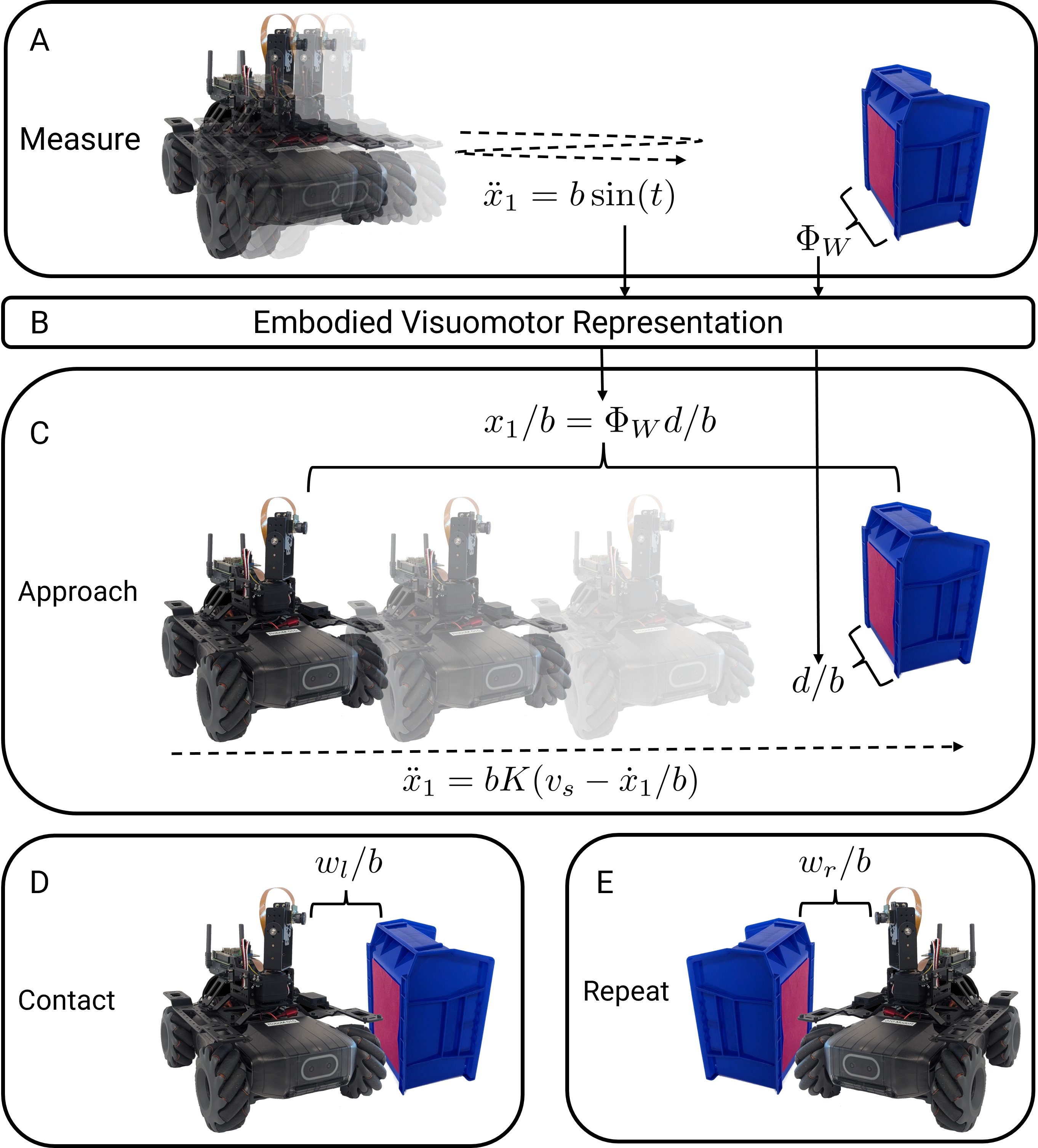
Figure 2: Overview of the procedure for uncalibrated touching using Embodied Visual Representation. (A): The robot oscillates by applying the control input $\sin(t)$ in open loop input measuring the size of the touching target in the visual field as $\Phi_{W}$. (B): Embodied Visuomotor Representation uses the control input and visual information to estimate the size $d$ and distance $x_{1}$ to the target in the embodied units $b^{-1}$. (C): With size of the target known, it is straightforward to approach the target at a constant speed using closed-loop control. In the closed loop, the effect of the unknown embodied gain $b$ cancels except for its interaction with the setpoint $v_{s}$. (D): Upon making contact with the target, the distance between the camera and target is the size of the body $w_{l}$ in the embodied unit. (E): The procedure can be repeated with different directions of approach to approximate the convex hull of the robot.

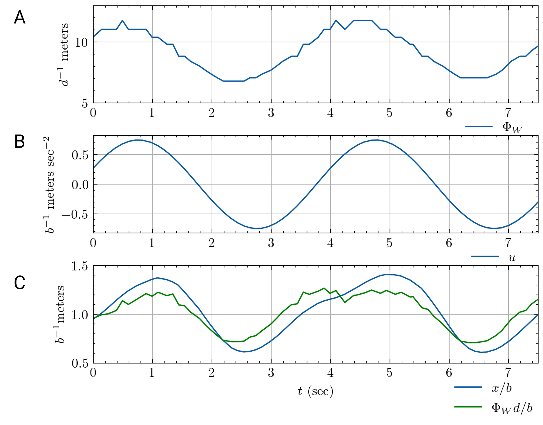
Figure 3: Experimental data and estimated signals from the measurement phase of uncalibrated touching (A): The size of the touching target in the visual field $\Phi_{W}$ as the robot oscillates. (B): The applied control input $u$, which is acceleration in the embodied unit $b^{-1}$. (C): The estimated distance from the visual target $x$ as estimated by the least squares problem and the implicitly estimated distance to the target resulting from multiplying the its estimated size $d$ by the size of the target in the visual field $\Phi_{W}$.

Contact with the object can be detected either with a touch sensor or by using the visual position estimate $\Phi_{W}d$ to detect that the robot has stopped getting closer to the target. Thus, the robot can approach a target at a constant safe speed in a given direction in the camera field, and touch it, regardless of the embodiment and environment’s specifications.

Uncalibrated Clearing

Once a robot can touch, it can quickly learn to clear obstacles as shown in Figure 4 and in Movie 1. In particular, it is possible to determine if it can fit through openings of unknown size prior to reaching them. Let the robot approach the touching target along direction $v$ in the body frame; then if the body extends further than the camera in the direction of $v$, the robot’s body will touch the target prior to the camera reaching the target. Let the time of contact be called $t_{c}$. At this time, the distance from the camera to the point on the body that is touching the target is $X(t_{c})/b$. Repeating the touching process by approaching a target from many directions allows the robot to approximate its convex hull in the scale of the embodied units.

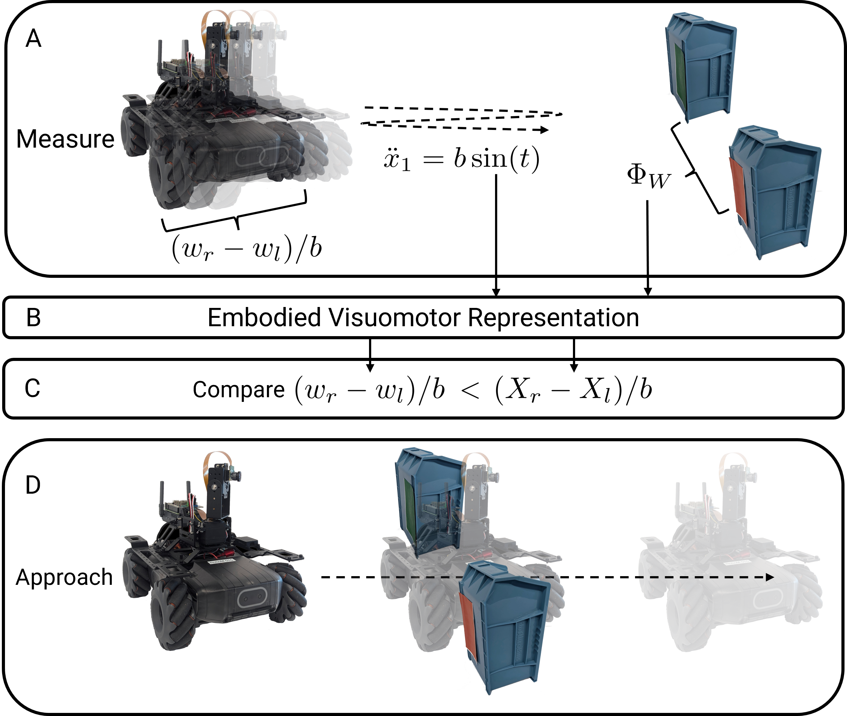
Figure 4: Overview of the procedure for clearing obstacles using Embodied Visual Representation. (A): The robot oscillates by applying the control input $\sin(t)$ in open loop input while measuring the size of the opening between two obstacles in the visual field as $\Phi_{W}$. (B): Embodied Visuomotor Representation uses the control input and visual information to an estimate the size of the opening, $X_{r}-X_{l}$, in the embodied units $b^{-1}$. (C): The size of the robot in the embodied unit, $(w_{r}-w_{l})/b$, as previously determined by uncalibrated touching, is compared to the size of the opening in the embodied unit to determine if the robot can fit, or clear, the opening. (D) If the robot can fit, the known size of the opening can be used to determine the position of the robot and closed-loop control can guide the robot through the opening.

Clearing obstacles is now as simple as measuring the distance from the robot’s camera to the object in the embodied unit and comparing that to the robots size in the embodied unit. In particular, if a robot has measured its width $w$ as $w/b$ in the embodied units through touch, then it only needs to measure the position of the left and right sides of an opening, take their difference, and compare to the width of the robot. Let the positions of the left and right sides of the opening be $X_{l}$ and $X_{r}$, then the robot measures their positions as $X_{l}/b$ and $X_{r}/b$, thus the robot fits if

$$w<\|X_{l}-X_{r}|\iff\frac{w}{b}<\left\|\frac{X_{l}}{b}-\frac{X_{r}}{b}\right\|.$$ (19)

Uncalibrated Jumping

Suppose an uncalibrated robot with two legs and a monocular camera needs to jump a gap to a platform an unknown distance away but at the same height. Let the legs applied force respond to inputs according to a first order low pass filter with a time constant $1/\alpha,\quad\alpha>0$. That is,

$$\begin{split}\ddot{X}&=bx_{act}-g\\ \dot{x}_{act}&=\alpha\left(u-x_{act}\right),\end{split}$$ (20)

where $g$ is a gravitational bias to be estimated. Then, let the robot fixate on an edge that it needs to jump past and oscillate up and down. During the oscillation, it collects measurements of the applied control inputs $u$ and the target line’s position along the vertical axis of the camera. Then (14) can be augmented with an additional gravitational bias term and then solved to estimate the actuator dynamics, the force of gravity, and the distance to the target line. Figure 5 illustrates this procedure and Figure 6 displays the collected visual data $\Phi_{W}$, control input $u$, and the estimated impulse response $g$ compared to the ground truth impulse response of the actuators.

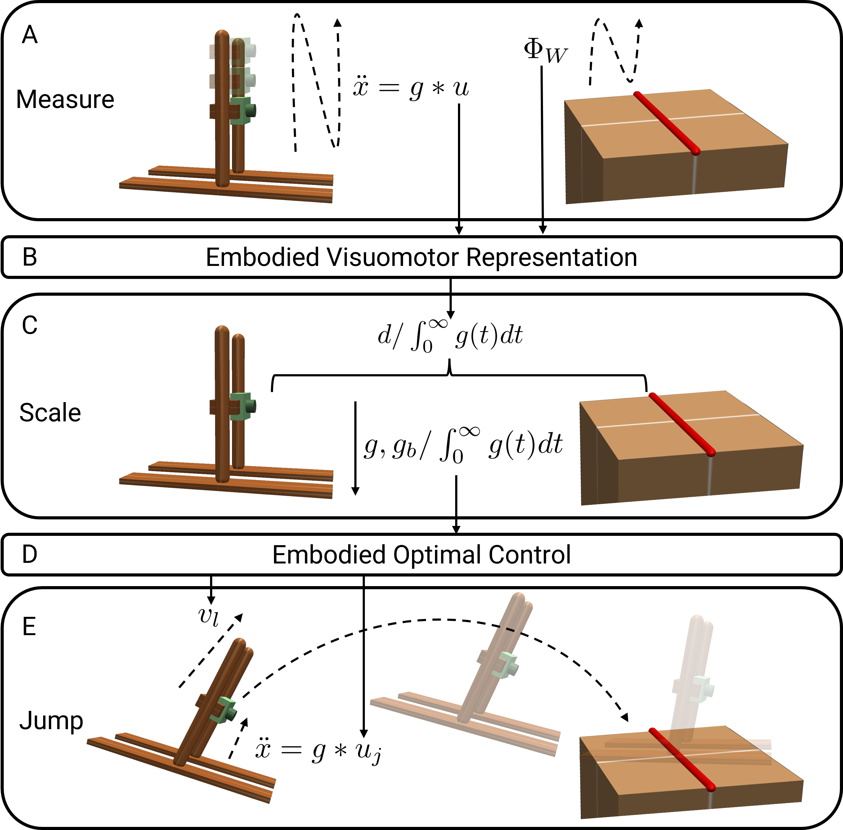
Figure 5: Overview of the procedure for jumping a gap using Embodied Visual Representation. (A): The robot oscillates up and down using a high gain control while measuring the control input $u$ and vertical position in the visual field $\Phi_{W}$ of a target line (red). The acceleration achieved $\ddot{x}$ results from filtering the control input by the unknown actuator dynamics $g$. (B), (C): Embodied Visuomotor Representation uses the control input and visual information to estimate the actuator dynamics $g$, distance to the jumping target $d$, and strength of gravity $g_{b}$ in the embodied units $\left(\int_{0}^{\infty}g(t)dt\right)^{-1}$. (D): An embodied optimal control problem is solved for the minimum first derivative control input $u_{j}$ that will reach the required launch velocity $v_{l}$ to jump the gap. (E) The jumping control input is executed in open loop after tilting the body forward.

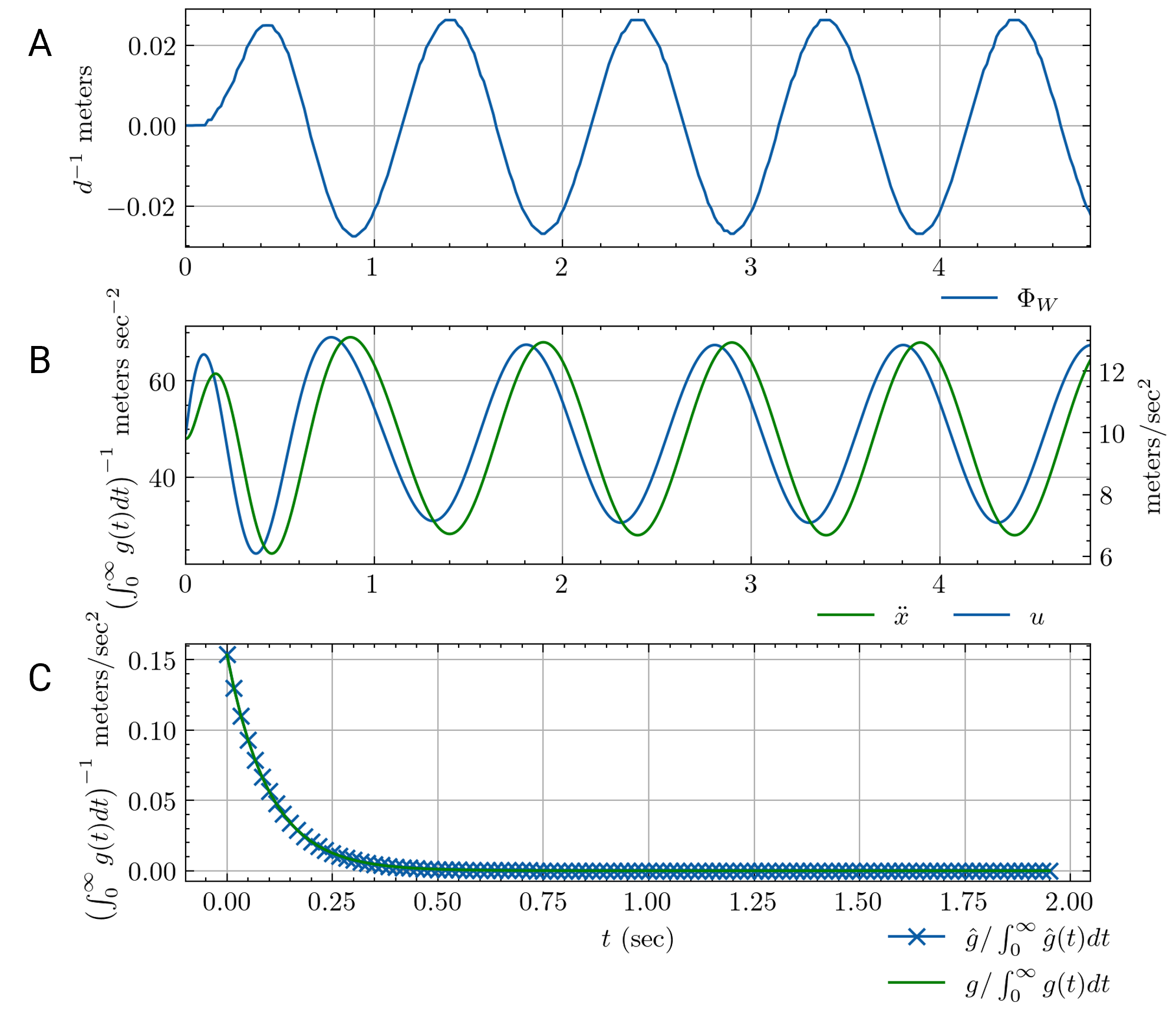
Figure 6: Experimental data and estimated signals from the measurement phase of uncalibrated jumping (A): The vertical position $\Phi_{W}$ of the target line as the robot oscillates up and down in preparation for jumping. (B): The applied control input $u$ in embodied units during the oscillation phase and the resulting acceleration $\ddot{x}$ in meters/second square. $\ddot{x}$ is phase shifted with respect to $u$ as result of the unknown actuator dynamics $g$. The magnitude is normalized due to the unknown embodied units. (C): The estimate of the impulse response of the actuator dynamics $\hat{g}$, resulting from applying Embodied Visuomotor Representation to the inputs $\Phi_{W}$ and $u$. $g$ is the ground truth impulse response. Both impulse responses are plotted in the embodied units of $\int_{0}^{\infty}\hat{g}(t)dt$ and $\int_{0}^{\infty}g(t)dt$ respectively.

Then given the embodied jumping distance $d$ (which happens to be the characteristic scale of vision), embodied gravity estimate, and prechosen launch angle $\theta_{l}$, the robot can solve the projectile motion equations to determine a launch velocity and the landing time $t_{f}$. The equations to be solved for $v_{l}$ and $t_{f}$ are:

$$\begin{split}0&=t_{f}\sin(\theta_{l})\dot{x}_{l}-\frac{1}{2}t_{f}^{2}g\\ d&=t_{f}\cos(\theta_{l})\dot{x}_{l}\end{split}$$ (21)

In the methods section, we detail an optimal control problem that can be solved via a quadratic program that minimizes the first derivative of a non-negative control input that can be applied to the leg actuators to reach the launch velocity.

So far, the mass of the robot’s legs and feet has been neglected as the effect of their mass on the jumping trajectory cannot be estimated by oscillating the body alone. For the purpose of this paper, it suffices to assume the mass of the legs and feet is small and so does not significantly affect the achieved jumping trajectory. However, the effect of the added mass of the legs and feet can be estimated by doing a vertical test jump prior to jumping the gap.

Comparisons to Bees and Gerbils

Next, we contrast the properties of algorithms using Embodied Visual Scale with behavior observed in bees and gerbils.

Bees have been recently shown to understand the size of an opening in wingbeats during their approach to an opening. It is thought that the size of the wings is learned during early development through contact with the hive. Additionally, the bees oscillate in an increasingly vigorous manner as openings are made smaller, seemingly to determine the size of the hole more accurately  (?). Our method for uncalibrated clearing determines the size of the robot in embodied units a priori through contact and is thus very similar. Additionally, it is clear from the least squares formulation that increased oscillation over longer periods will increase the accuracy of the estimated quantities by decreasing the condition number of the independent variables and averaging out the effects of noise.

Similarly, Mongolian Gerbils vibrate their body up and down before making a jump over a gap of unknown distance. It is thought that this helps their visuomotor system determine appropriate muscle stimulation to clear the gap  (?). Like bees, the intensity of the oscillations increases when the gap is larger and thus more difficult to jump. Our approach also requires oscillation, can estimate the appropriate actuator stimulation to jump a gap, and theoretically benefits from higher frequency oscillations over longer timer intervals.

Discussion

It has been shown that Embodied Visuomotor Representation allows an uncalibrated robot, without any knowledge of distance, to accomplish tasks such as touching, clearing, and jumping with theoretically guaranteed stability. This is accomplished by exchanging units in an external scale, such as the meter, for the implicitly defined distance unit associated with the robot’s acceleration in response to a control input and observed in a unit-less quantity by vision. The resulting algorithms have a different architecture from the traditional sense-plan-act cycle as contrasted in Figure 1.

It must be acknowledged that body-length units, such as the lengths of the body itself, have long been posited as a natural source of embodied scale. Indeed such units are useful for many applications. However, body length units are not directly available in the equations above (they are encoded in $\theta$). Regardless, our representation is not incompatible with frameworks based on body-length units. Instead, it provides a method for a robot to estimate or re-estimate body-length units as needed.

We further compare traditional approaches based on sense-plan-act with our approach based on Embodied Visuomotor Representation in Table 1. The table compares the main algorithmic components of traditional approaches that might be used to achieve touching, clearing, and jumping. This comparison reveals how the stability of traditional approaches becomes implicitly tied to a priori knowledge of the conversion factor between an embodied scale and an external scale. Fundamentally, this is because it is traditional to assume the availability of low-level controllers that accept inputs on an external scale. However, this assumption implicitly absorbs the conversion from the external scale to the embodied scale into the controller. In the end, this makes the closed loop gain and overall stability of any task dependent on the conversion factor.

Task	External Scale	Embodied Visuomotor Representation (EVR)
Touching	State estimated with calibrated sensors in external scale Control stabilizes state via conversion to embodied signals Stability depends on a priori knowledge of conversion factor	Embodied state estimated with EVR Control stabilizes embodied state with embodied signals Stability is invariant to units
Clearing	Robot’s physical size defined in external scale State estimated with calibrated sensors in external scale The clearing algorithm uses a world in an external scale and clears objects via conversion to embodied signals Stability depends on conversion and a pre-determined physical model	Embodied physical size estimated with touch Embodied state estimated with EVR The clearing algorithm uses an embodied world that is consistent with embodied signals Stability is invariant to units and physical dimensions
Jumping	Jumping distance estimated using calibrated sensors Launch velocity estimated in external scale Control achieves launch velocity via conversion to embodied signals Success dependent on scale and pre-determined controller	Jumping distance and actuator dynamics estimated with EVR Launch control signal estimated via embodied representation Launch control signal applied open loop Stability invariant to units and controller

Table 1: Robot behaviors that can be accomplished with external scale and traditional methods, but can also be accomplished with Embodied Visuomotor Representation (EVR). Due to its use of embodied scale Embodied Visuomotor Representation theoretically guarantees success and stability without calibrated sensors, pre-determined physical models, and low-level controllers that are tuned prior to deployment.

The development of Embodied Visuomotor Representation has borrowed ideas broadly from many areas, in particular the Tau Theory, Glenberg’s theory of Embodiment as Memory, the Internal Model Priniciple, and Visual Self-Models. Below, these frameworks are compared and contrasted to Embodied Visuomotor Representation. We further compare our framework to leading approaches in robotics, including Visual Inertial Odometry (VIO), Visual Self-Modeling, and Deep Visuomotor Control.

Before launching into these specific comparisons, recall that Embodied Visuomotor Representation is a concrete methodology, realized through engineering principles, that allows robots to emulate a phenomenon well known in the sciences. This phenomenon does not necessarily allow robots to do tasks they could not do before; rather, it makes it significantly easier for them to do any given task. This is because low-level control laws become self-tuning, detailed physical models are not needed, and 3D sensors do not need to be calibrated.

Comparisons to existing frameworks

Tau Theory (Time-to-contact)

One of the first works in psychology to consider how the scale-less quantities available to the visual system could be used by humans for embodiment control was the Tau Theory  (?). In this work control goals based on time-to-contact ($\tau$) are proposed that allow a driver of a car to avoid hitting another car. Over the years, this was developed into the “General Tau Theory”  (?) which aims to explain how numerous types of behaviors exhibited by animals and humans can be explained in terms of the time-to-contact (tau) signals observed during the behavior.

Tau theory generally proposes that certain tau trajectories should be achieved without providing a specific control law in terms of forces and with consideration of the dynamics of the system that can execute the desired tau trajectory. Roboticists must implement specific control laws, and thus there have been many proposed that use time-to-contact as the basis for biologically inspired robot control. Some examples include  (?), which discusses landing a spacecraft using time-to-contact,  (?), which uses a depth camera and $\tau$ to avoid objects, and  (?), which uses time-to-contact to derive a rigorous control law that lands on moving platforms. However, formulations that use time-to-contact directly for control are known to be sensitive to time delay  (?). In  (?), this was overcome with an oscillation-based strategy that measured distance through a qualitative process based on observing oscillations and reducing the control gain.

Tau is also known to quantitatively relate distance and acceleration in an equality constraint. In  (?) this is used in a form relating time-to-contact, its derivative, acceleration, and distance in an instant of time. Further, in  (?), the solution of the linear-time-varying system defined by time-to-contact is used to evaluate the trajectories up to an unknown initial distance. Similarly,  (?) used an extended Kalman filter to fuse control effort and time-to-contact to measure distance and do closed-loop control. In  (?), the solution is used to estimate distance using an IMU and a camera with a sliding window-based optimization.

Embodied Visuomotor Representation can use time-to-contact as the basis for a scaleless visual transition matrix $\Phi_{W}$ as in  (?) without committing to any particular control law. Further, it is easy to use the framework to verify if a proposed control law is stable. Finally, while only equality constrained Embodied Visuomotor Representation was developed in this paper, inequality constraint forms clearly exist and may be developed further to realize rigorous versions of the qualitative control laws observed in psychology and developed in robotics.

Memory as Embodiment

Glenberg’s theory of memory as embodied representations  (?) is tightly coupled to our theory of Embodied Visuomotor Representation. Glenberg writes, “embodied representations do not need to be mapped onto the world to become meaningful because they arise from the world” and our proposed Embodied Visuomotor Representation does just that, thus realizing guaranteed stability despite having no explicit knowledge of scale.

A core tenet of Glenberg’s theory is the “merge” operation that allows memories of different types of actions to be combined to do a new task. However, no specific examples for merging motion are given. On the other hand, our Embodied Visuomotor Representation admits a path towards a general motion based “merge” operator because it explicitly represents the systems dynamics. Consideration of this path, which may allow adding attributes such as “carefully” to “navigate through an opening”, will be considered in future work.

Internal Model Principle

The Internal Model Principle is a long standing principle in control theory that suggests an internal model of the process to be regulated must be contained within a controller if it is to succeed. This principle has analogs in many fields especially psychology, where it has been accepted that internal models are developed and used by humans to control themselves effectively. This idea also made its way to computer science, where Animate Vision was proposed as a way to explain how vision and control can be formulated as a single sensorimotor process with minimal internal representation  (?, ?). Both the Internal Model Principle and the Animate Vision approach bypass the sense-plan-act paradigm common in computer vision and robotics today, which attempts to represent every part of the world concretely up to the small details, using a layered processing architecture  (?).

One of the more exciting recent applications of the internal model principle in neuroscience is the discovery that dragonflies have a visuomotor internal model  (?, ?). Specifically it was found that an internal model is used to compensate for time delays in the dragonflies nervous system so that the dragonfly can keep a target foveated during target interception.

Prior to the findings about dragonflies, there were many studies on humans supporting the existence of internal models in humans. One of the seminal works is  (?), which showed that humans likely have an internal model for the prediction of arm position. Further, the authors were able to explain experimental data’s qualitative characteristics using a Kalman filter based model. These findings were further developed over multiple decades, resulting in the hypothesis that the internal models in humans are ultimately Bayesian and are utilized mainly for the purposes of optimal and robust control  (?).

These theories are very general, and so they do not explicitly consider the visuomotor control problem and the problems introduced by the unit-less representation of space admitted by visual processes. Thus, Embodied Visuomotor Representation can be seen as a specialization of the Internal Model Principle specifically for visuomotor processes that do not have access to an external scale but still need to represent themselves in a unit.

Visual Self-Modeling

Recently, representations for self-modeling have been proposed that represent a robot’s 3D form using neural networks  (?). The approach depends on externally calibrated 3D stereo cameras to scan the robot in different configurations. Neural networks then predict the robot’s occupancy map to scale as a function of the robot’s joint angle configuration. The resulting representation is useful for many tasks, such as touching and determining if the robot is damaged, and it is suggested that the representation may also be used for determining if a robot will fit through an opening.

Embodied Visuomotor Representation is, in theory, compatible with the 3D self-modeling representation proposed by  (?). However, instead of 3D scans provided by external stereo cameras, touching can be used to learn the robot’s morphology, and a single onboard monocular camera suffices, as demonstrated. Thus, future work can consider training Visual Self-Models via Embodied Visuomotor Representation. Further, the combination will allow self-modeling of robots that translate, and are thus governed by unstable second order integrators, as opposed to robots whose configuration space is bounded via a list of joint angles.

Deep Visuomotor Control

The field of deep neural network based visuomotor control is exemplified by  (?). In such works, a neural network is trained for tasks whose completion can be measured visually, such as placing a cube in a box, and the neural network must directly output motor commands or setpoints for lower-level controllers. Recent work has considered visual navigation, where a robot must learn to navigate through a scene from visual inputs and output concrete actions to be taken by low-level controllers  (?). Later work considers training the network on a variety of morphologies so that a single representation can control a variety of robots via an existing low-level controller despite differences in physical shape  (?)  (?).

Due to its architecture, Deep Visuomotor Control results in an end-to-end algorithm that is good for complex tasks provided a sufficient number of training examples are available. In contrast, Embodied Visuomotor Representation is a low-level representation that needs only a few samples to learn to control a particular embodiment and roughly represent its morphology. Thus, Embodied Visuomotor Representation can be used as an underlying scheme for training high-level schemes based on Deep Visuomotor Control.

Visual Inertial Odometry

In the field of Visual Inertial Odometry, inertial measurement units (IMUs) are fused with visual perception to estimate the metric trajectory of a robot in meters. While this is not strictly visuomotor, it is closely related since forces are ultimately exerted by a motor system to affect an observer’s motion. An early approach was the Multi-State Constraint Kalman Filter  (?). This was followed by ROVIO, which used a patch-based formulation that directly operated on image intensities. Later, VINS-MONO  (?) introduced a sliding window-based formulation that avoids the need for good initialization. The prevailing methods in VIO continue to follow the architecture of these approaches.

These methods typically follow a match, estimate, and predict architecture based on matching features to get a dimensionless estimate of the robot’s trajectory. Architecturally, this is identical to sense-plan-act but in the estimation setting. The features are tracked across a wide field-of-view and so independent motion detection methods have to be added in order to deal with non-static scenes.

In contrast, Embodied Visuomotor Representation explicitly considers the characteristic scale of vision, which may not be the distance to features considered by VIO. In particular, it can be the scale of the geometry of an object under fixation. This results in an object-centered visual framework where control tasks are considered with respect to individual objects instead of a global world frame.

Despite these differences IMU’s are still useful for future work in Embodied Visuomotor Representation. As already noted, they are useful for making visual estimates’ rotation invariant for short periods of time. Further, their acceleration can be used up to scale to better estimate mechanical parameters. They also allow a robot to learn the conversion factor between its embodied scale and an external scale. This factor can be used by higher-level processes that may need to maintain safe distances or velocities as might be mandated by a safety standard even as the robot’s mechanical properties change over time.

Future Work

The above comparisons to existing concepts resulted in several directions for future work, including forward prediction, incorporation of IMUs to meet safety standards, and training neural networks. However, there are many more, and so below, we outline the future work in theory and applications that we consider most important.

Theory

This paper has considered only equality-constrained Embodied Visuomotor Representation. That is, the unitless quantities from vision are considered to exactly equal some operator of control inputs. Ideas from Psychology, and, in particular, the Tau theory, suggest that more qualitative processes will suffice for many applications. Thus, it is of interest to develop inequality-constrained Embodied Visuomotor Representation in hopes of realizing qualitative representations and qualitative control laws that robots can use to accomplish tasks.

Turning back to equality-constrained Embodied Visuomotor Representation, we have presented two types of estimation problems. The first, exemplified by (9), estimates quantities in embodied units of action. The second formulation is given by (14) and estimates quantities in units of the visual processes characteristic scale. Subsequently, these quantities can be converted to an embodied unit of action. An immediate question is then which formulation is better. Further, error characterization of Embodied Visuomotor Representation should be performed so that optimal Embodied Visuomotor Representation estimators can be realized.

Next, we discuss dynamics representation. The derivation of Embodied Visuomotor Representations above neglected damping and spring effects as might be caused by friction or tendon-like attachments, respectively. However, these effects can be incorporated, assuming these naturally occurring dynamics are stable, which they almost always will be. For example, we can incorporate into an Embodied Visuomotor Representation a system’s dissipating energy due to spring and damping effects by considering velocity or position as the fundamental quantities controlled by the action instead of acceleration. In this paper, acceleration was used as the fundamental quantity controlled through action because many animals and robots do not experience significant sliding friction or spring effects that are coupled with their position.

Finally, it is interesting to consider more general dynamics than linear systems and how to control them via Embodied Visuomotor Representation. In principle, except for the use of unit-less visual feedback, this is not substantially different from existing work in robot dynamics, and we expect many techniques to port over directly. On the other hand, the linear dynamics considered in this paper should be sufficient for many applications. Thus, it is of interest to apply recent advancements in adaptive control, such as kernel methods that guarantee estimation of BIBO stable impulse responses  (?).

Applications

The most straightforward future work that can be accomplished via Embodied Visuomotor Representation is avoiding and pursuing (or catching) dynamic objects. The basic procedure is identical to the touching, clearing, and jumping tasks, except that an additional model of the dynamic object must be considered.

We also consider imitation and embodied affordance estimation to be the next two most important applications. Assuming the embodied mechanical and dynamics parameters have already been estimated, imitation within Embodied Visuomotor Representation becomes a problem of determining the embodied control signals that accomplish a visually observed behavior. The characteristic scale-based representation of vision will then naturally allow robots to imitate an action using the units of their own embodiment instead of an external scale.

Finally, while this paper has exclusively considered visual processes and their connection to motor signals, the basic principles should be extended to consider touch and audio. We are particularly interested in touch sensing because touch is an action that causes visual responses that can be modeled in the existing framework.

Materials and Methods

Hardware

The robot platform used for the touching and clearing experiments is a DJI RoboMaster EP. The platform features mecanum wheels, which allow it to translate omnidirectionally. The provided robot arm and camera were removed and replaced with a pan-tilt servo mount and a Raspberry Pi Camera Module 3 with a wide-angle lens. A Raspberry Pi 4 was attached to the camera to interpret images at a target rate of 20 frames per second and provide control commands to the robot.

The DJI RoboMaster does not support direct acceleration control. The lowest level supported is velocity control. To emulate the double integrator described in the touching and clearing experiments, the acceleration commands from the proposed control laws were transformed into velocity commands using a leaky integrator with a time constant of $2/3$ seconds.

Uncalibrated Touching

The touching experiment uses color thresholding to detect the pixels of a planar target. Assuming the robot is facing the planar target, the width in normalized pixels in the visual field is then taken as the characteristic scale of vision $d$. The robot oscillates in open-loop by applying a $0.25$ Hz sinusoidal acceleration signal over a $15$ second interval. A least squares estimation problem is used to solve the current position, velocity, and size of the touching target in embodied units using a 5 second sliding window of measurements.

Subsequently, the robot drives toward the target at a constant velocity of $0.2$ embodied units per second for a duration $10\%$ longer than that required to traverse the initial distance between the robot and the target. Consequently, the robot makes contact with the target. The minimum distance between the robot’s camera and the target is then the horizontal distance between the robot’s camera and the edge of the robot that made contact with the target first.

Uncalibrated Clearing

The clearing experiments consider if the robot can fit through an opening (clear it) prior to reaching the opening. To do so, the robot determines the width of the body in the embodied unit by touching its left and right sides to a nearby object using the previously described procedure. It remains for the robot to measure the size of an opening in the embodied unit. Once again, the left and right sides of the opening are detected with color thresholding. The left and right edges of the right and left sides of the opening, respectively, are used as the characteristic scale of vision. A 7.5 second, 0.25 Hz open loop sinusoidal acceleration is applied and a sliding window estimator using 5 seconds of data subsequently estimates the size of the opening in the embodied units.

If the robot is smaller than the opening, it proceeds through with PID-based position control, where the distance between the robot and the opening is measured using the estimated characteristic scale and vision.

Uncalibrated Jumping

The jumping robot experiment was performed in a MuJoCo simulation  (?). Codes for this simulation are provided in the supplemental materials.

The robot consists of a body on two legs and feet. The legs are modeled as cylinders or pistons, with first-order activation dynamics and a time constant of 0.1 seconds. The body mass was set to 10 kg, and the mass of the legs and feet amounted to 0.22 kg. Two angular position controllers hold the legs upright during the measurement phase of the experiment and tilt the body forward approximately 20 degrees during the jumping phase.

The measurement phase of the jumping experiment consists of three parts. In the first, the minimum/maximum position of the body are estimated by recording the initial position as the bottom position, increasing the upwards force until the body begins to lift, initializing a PID controller’s integrator term with the force that overcomes gravity, and subsequently using PID control to maintain a constant upwards velocity until the top position is reached. Subsequently, the PID controller oscillates the body for $5$ seconds at $1$ Hz around the midpoint between the bottom and top positions with an amplitude equal to $1/4$ of the distance between the top and bottom positions.

During oscillation, color thresholding is used to determine the vertical normalized pixel coordinate corresponding to a red line placed in the middle of the target platform. The characteristic scale of vision then becomes the distance between the robot and the red line. Subsequently, the measurements of the control effort applied by the PID control and the vertical normalized pixel coordinate are used to solve for the leg actuator’s impulse response, the distance between the robot and the red line, and the initial velocity.

To approximate the actuator impulse response, a linear combination of $1000$ first-order impulse responses truncated to 2 seconds with initial magnitude equal to $1$ and time constants ranging from $0.0001$ to $1$ second are considered. The resulting quadratic program to estimate the distance to the line, initial velocity, and actuator dynamics is then given by:

$$\begin{split}&\min_{\frac{\dot{X}_{2}(0),g_{b},c}{d}}\int_{2}^{T}\left(\Phi_{W}(t)-t\frac{\dot{X}_{2}(0)}{d}-\frac{1}{2}\frac{g_{b}}{d}t^{2}-\frac{g}{d}*\int_{0}^{t}\int_{0}^{\sigma}u(\sigma_{2})d\sigma_{2}d\sigma\right)^{2}dt\\ &\frac{g(t)}{d}=\sum_{i}c_{i}e^{-t/\tau_{i}}\\ \mathrm{s.t.}&\quad c_{i}>=0\quad\forall i\end{split}$$ (22)

where $\dot{X}_{2}(0)$ is the initial velocity on the robot camera’s vertical axis, $g_{b}$ is the gravitational bias force, $c_{i}$ are the coefficients of the basis functions for $g$ and $\tau_{i}$ are the corresponding time-constants of the basis functions. The double integral is computed using a $0.001$ second approximation, corresponding with the simulation’s timestep. The outermost integral is approximated with a $1/60$’th of a second timestep, corresponding to the 60 fps simulated camera. The loss is evaluated over the interval $[2,T]$ instead of $[0,T]$ to prevent initial conditions from contributing to the actuator dynamics through the 2 second long impulse response $g$. Non-negativity of $c_{i}$ is necessary to prevent overfitting to numerical integration errors.

To convert from units of the characteristic scale to embodied units of action, we divide each estimated quantity by $\int_{0}^{\infty}g(t)dt/d$ as described previously. In what follows all quantities can be assumed to be in this embodied unit.

Subsequently, the standard equations for projectile motion are combined with the estimated embodied distance and gravitational force to solve for an embodied launch velocity that will jump the gap. A terminally constrained optimal control problem is solved to find the control input with a minimum first derivative that accelerates the body from rest to the launch velocity over the distance oscillated during the measurement phase at the end of a pre-chosen launch interval of $T=250$ millisecond. The resulting quadratic program is:

$$\begin{split}&\min_{u}\int_{0}^{T}\left(\frac{d}{dt}u(t)\right)^{2}dt\\ \mathrm{s.t.}&\int_{0}^{T}(g*u)(t)dt=v_{l}\\ &\int_{0}^{T}\int_{0}^{\sigma}(g*u)(\sigma_{2})d\sigma_{2}d\sigma=d_{m}\\ &u(0)=0,\quad u(T)=0,\quad u(t)>=0,\quad\forall t\in[0,T]\end{split}$$ (23)

where $v_{l}$ is the necessary launch velocity in embodied units, and $d_{m}$ is the distance from the start position at which the launch velocity should be achieved. $d_{m}$ is necessary to ensure the launch velocity is reached prior to reaching the maximum position of the body with respect to the legs. Non-negativity of $u$ is required to prevent lifting the lightweight legs from the jumping platform prior to reaching the launch velocity. We formulate and solve the problem using a discrete time approximation of $0.001$ seconds. Because of exponential decay, $(g*u)(t)>0$ when $t>T$ and so the leg actuators are deactivated for $t>T$ to prevent the bodies velocity from exceeding $v_{l}$. The resulting embodied jump control signal $u$ is offset by the estimated gravitational bias and executed in an open loop.

Data Availability

Videos are provided in the supplementary information and at prg.cs.umd.edu/EVR.

Code Availability

Code for the jumping simulation is provided in the supplementary information and at prg.cs.umd.edu/EVR. Codes for the touching and clearing experiments are available upon reasonable request.

Contributions

L.B. conceived and developed the mathematics for Embodied Visuomotor Representation, designed the algorithms solving the uncalibrated touching, clearing, and jumping problems, built the robot, wrote software, performed experiments, and wrote the manuscript. C.F. connected the ideas to existing literature and helped write the manuscript. Y.A. posed the questions answered by Embodied Visuomotor Representation, connected it to existing literature, and helped write the manuscript. All authors read and approved the final manuscript.

Competing interests

The authors declare no competing interests.

Supplementary material

The supplementary figures below compare the achieved jumping trajectories to the theoretical trajectories when the simulation parameters are varied. Figure 7 compares target jump distances of 3, 4, and 5 meters. Figure 8 shows how the jumping excitation signal $u$ changes as function of these distances. Figure 9 compares body masses of 5, 10, and 15 kilograms. Figure 10 compares actuator time-constants of 5, 10, and 20 milliseconds.

Movie 2 shows a jump achieved with the nominal parameters detailed in the Materials and Methods section. Additionally, the source code for the jumping simulation is provided in the supplementary materials.

Figure 7: Theoretically optimal jump trajectory versus achieved jump trajectory for jumps of 3 meters, 4 meters, and 5 meters in distance. The distance jumped remains consistent with the theoretically expected jump.

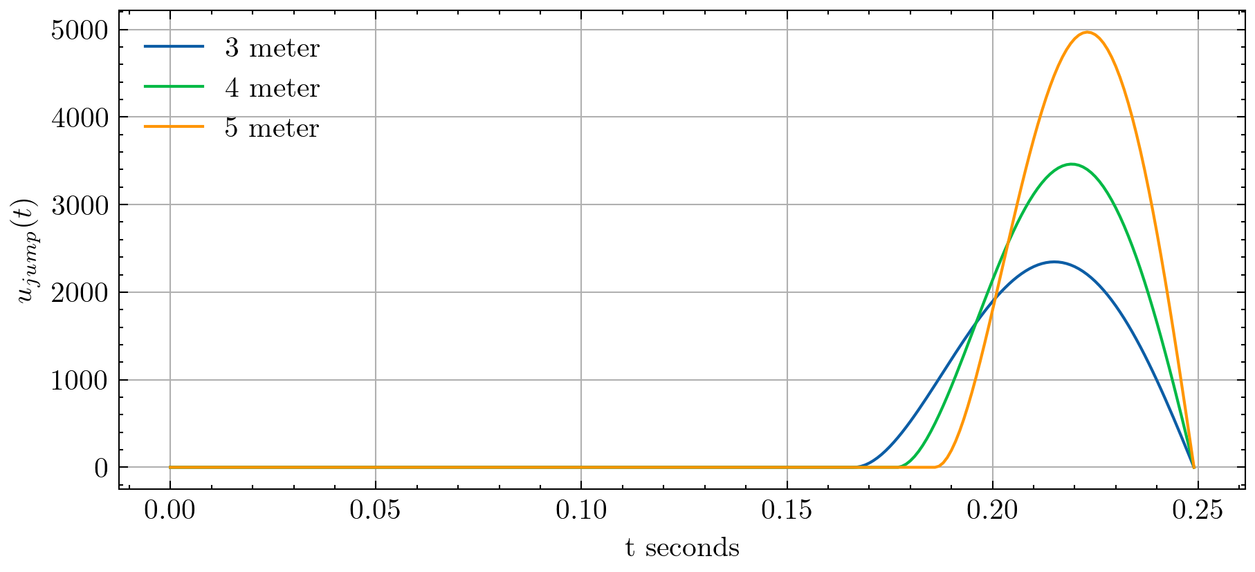
Figure 8: Jump exciting signal resulting from the embodied optimal control problem for the best jumping control input for jumps of distance 3 meters, 4, meters, and 5 meters in distance.

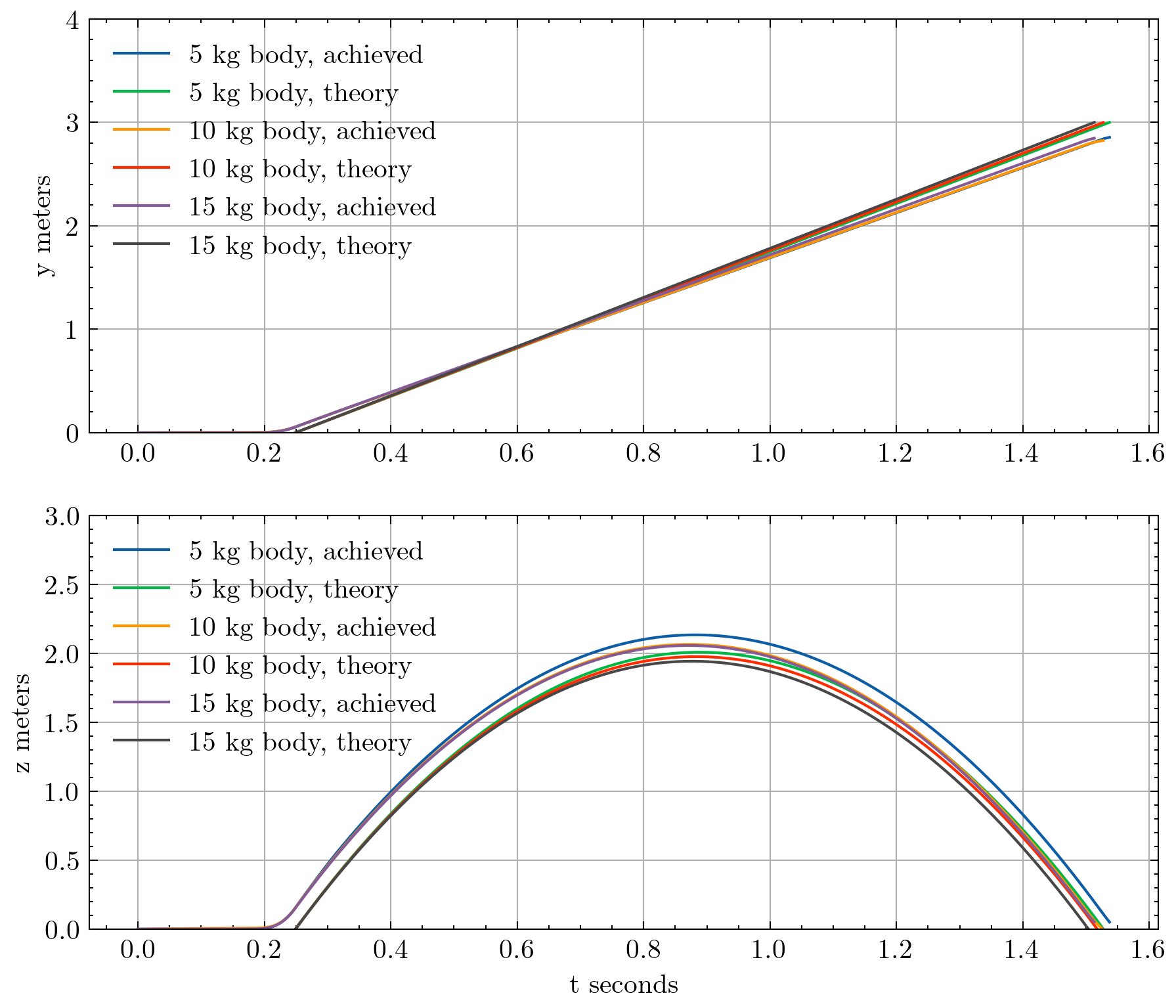
Figure 9: Theoretically optimal jump trajectory versus achieved jump trajectory for jumps of 5 meters with a body mass of 5, 10, and 15 kilograms. The distance jumped remains consistent with the theoretically expected jump.

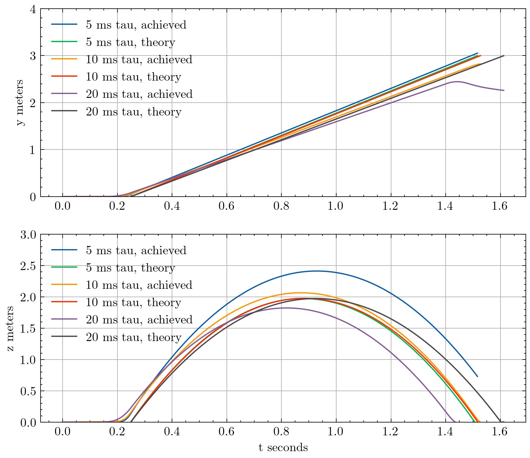
Figure 10: Theoretically optimal jump trajectory versus achieved jump trajectory for jumps of 5 meters with a actuator first order time-constant of 5, 10, and 20 milliseconds. When varying the time-constant, the achieved jumping trajectory is not as consistent with the theoretical trajectory as when varying jumping distance and mass. However, this can be explained by considering that the integration dynamics of the leg actuators are not exact, and so it is expected that there will be some differences between the estimated actuator dynamics and the simulated actuator dynamics which will result in minor variations in the jumping trajectory.

References

- 1. D. Marr, Vision: A computational investigation into the human representation and processing of visual information (MIT press, 2010).
- 2. J. Aloimonos, I. Weiss, A. Bandyopadhyay, Active vision, International Journal of Computer Vision 1, 333–356 (1988).
- 3. R. Bajcsy, Y. Aloimonos, J. K. Tsotsos, Revisiting active perception, Autonomous Robots 42, 177–196 (2018).
- 4. D. H. Ballard, Animate vision, Artificial Intelligence 48, 57-86 (1991).
- 5. Mars Climate Orbiter Mishap Investigation Board, Phase I report, National Aeronautics and Space Administration (1999).
- 6. J. A. Feldman, Four frames suffice: A provisional model of vision and space, Behavioral and Brain Sciences 8, 265–289 (1985).
- 7. J. J. Koenderink, A. J. Van Doorn, A. M. Kappers, Surface perception in pictures, Perception & Psychophysics 52, 487–496 (1992).
- 8. J. T. Todd, The visual perception of 3D shape, Trends in cognitive sciences 8, 115–121 (2004).
- 9. L. Cheong, C. Fermüller, Y. Aloimonos, Effects of errors in the viewing geometry on shape estimation, Computer Vision and Image Understanding 71, 356–372 (1998).
- 10. H. Ji, C. Fermüller, Noise causes slant underestimation in stereo and motion, Vision Research 46, 3105–3120 (2006).
- 11. S. Ravi, et al., Bumblebees perceive the spatial layout of their environment in relation to their body size and form to minimize inflight collisions, Proceedings of the National Academy of Sciences 117, 31494–31499 (2020).
- 12. M. Mischiati, et al., Internal models direct dragonfly interception steering, Nature 517, 333–338 (2015).
- 13. C. G. Ellard, M. A. Goodale, B. Timney, Distance estimation in the mongolian gerbil: The role of dynamic depth cues, Behavioural brain research 14, 29–39 (1984).
- 14. A. M. Glenberg, What memory is for, Behavioral and Brain Sciences 20, 1–19 (1997).
- 15. O. Brock, Intelligence as computation, arXiv preprint arXiv:2405.16604 (2024).
- 16. D. McNamee, D. M. Wolpert, Internal models in biological control, Annual Review of Control, Robotics, and Autonomous Systems 2, 339-364 (2019).
- 17. J. Huang, et al., Internal models in control, biology and neuroscience, 2018 IEEE Conference on Decision and Control (CDC) (2018), pp. 5370–5390.
- 18. K. Åström, B. Wittenmark, Adaptive Control, Dover Books on Electrical Engineering (Dover Publications, 2008).
- 19. L. Burner, N. J. Sanket, C. Fermüller, Y. Aloimonos, TTCDist: Fast distance estimation from an active monocular camera using time-to-contact, 2023 IEEE International Conference on Robotics and Automation (ICRA) (2023), pp. 4909–4915.
- 20. D. N. Lee, A theory of visual control of braking based on information about time-to-collision, Perception 5, 437–459 (1976).
- 21. D. N. Lee, R. J. Bootsma, M. Land, D. Regan, R. Gray, Lee’s 1976 paper, Perception 38, 837-858 (2009).
- 22. O. Sikorski, D. Izzo, G. Meoni, Event-based spacecraft landing using time-to-contact, Proceedings of the IEEE/CVF Conference on Computer Vision and Pattern Recognition (CVPR) Workshops (2021), pp. 1941–1950.
- 23. C. Walters, S. Hadfield, EVReflex: Dense time-to-impact prediction for event-based obstacle avoidance, 2021 IEEE/RSJ International Conference on Intelligent Robots and Systems (IROS) (2021), pp. 1304–1309.
- 24. B. Herissé, T. Hamel, R. Mahony, F.-X. Russotto, Landing a VTOL unmanned aerial vehicle on a moving platform using optical flow, IEEE Transactions on Robotics 28, 77-89 (2012).
- 25. G. C. H. E. de Croon, Monocular distance estimation with optical flow maneuvers and efference copies: a stability-based strategy, Bioinspiration & Biomimetics 11, 016004 (2016).
- 26. D. Izzo, G. Croon, Nonlinear model predictive control applied to vision-based spacecraft landing, 2013 EuroGNC (2013).
- 27. H. W. Ho, G. C. de Croon, Q. Chu, Distance and velocity estimation using optical flow from a monocular camera, International Journal of Micro Air Vehicles 9, 198–208 (2017).
- 28. D. H. Ballard, C. M. Brown, Principles of animate vision, CVGIP: Image Understanding 56, 3-21 (1992). Purposive, Qualitative, Active Vision.
- 29. D. M. Wolpert, Z. Ghahramani, M. I. Jordan, An internal model for sensorimotor integration, Science 269, 1880-1882 (1995).
- 30. B. Chen, R. Kwiatkowski, C. Vondrick, H. Lipson, Fully body visual self-modeling of robot morphologies, Science Robotics 7, eabn1944 (2022).
- 31. S. Levine, C. Finn, T. Darrell, P. Abbeel, End-to-end training of deep visuomotor policies, The Journal of Machine Learning Research 17, 1334–1373 (2016).
- 32. D. Shah, B. Eysenbach, G. Kahn, N. Rhinehart, S. Levine, Ving: Learning open-world navigation with visual goals, 2021 IEEE International Conference on Robotics and Automation (ICRA) (2021), pp. 13215–13222.
- 33. D. Shah, A. Sridhar, A. Bhorkar, N. Hirose, S. Levine, Gnm: A general navigation model to drive any robot, 2023 IEEE International Conference on Robotics and Automation (ICRA) (2023), pp. 7226–7233.
- 34. D. Shah, et al., ViNT: A foundation model for visual navigation, 2023 Conference on Robot Learning (CoRL) (2023).
- 35. A. I. Mourikis, S. I. Roumeliotis, A multi-state constraint Kalman filter for vision-aided inertial navigation, Proceedings of the 2007 IEEE International Conference on Robotics and Automation (2007), pp. 3565–3572.
- 36. T. Qin, P. Li, S. Shen, VINS-Mono: A robust and versatile monocular visual-inertial state estimator, IEEE Transactions on Robotics 34, 1004–1020 (2018).
- 37. M. Bisiacco, G. Pillonetto, On the mathematical foundations of stable RKHSs, Automatica 118, 109038 (2020).
- 38. E. Todorov, T. Erez, Y. Tassa, Mujoco: A physics engine for model-based control, 2012 IEEE/RSJ International Conference on Intelligent Robots and Systems (IEEE, 2012), pp. 5026–5033.
Acknowledgments
The support of NSF award OISE 2020624 is gratefully acknowledged. The authors thank Rohit Kommuru for prototyping early versions of the jumping experiment.