Abstract

A systematic construction for supersymmetric negative (non-local) flows for mKdV and KdV based on $sl(2,1)$ with a principal gradation is proposed in this paper. We show that smKdV and sKdV can be mapped onto each other through a gauge super Miura transformation, together with an additional condition for the negative flows, which ensure the supersymmetry of the negative sKdV flow. In addition, we classify both smKdV and sKdV flows with respect to the vacuum (boundary) solutions accepted for each flow, whether zero or non-zero. Each vacuum is used to derive both soliton solutions and the Heisenberg subalgebra for the smKdV hierarchy, where we present novel vertex operators and solutions for non-zero bosonic and fermionic vacuum. Finally, the gauge Miura transformation is used to obtain the sKdV solutions, which exhibit a rich degeneracy due to both multiple gauge super Miura transformations and multiple vacuum possibilities.

1 Introduction

Integrable field theories are very peculiar models admitting infinite number of conservation laws. These are, in turn responsible for the stability of soliton solutions. The Korteweg–de Vries (KdV) [1, 2, 3] and modified KdV (mKdV) [4, 5] equations are for instance, typical examples of such a class of models and have acted as prototypes for many new developments in the subject. More recently integrable hierarchies appears in many areas of theoretical physics, as in 2D CFTs [6, 7, 8, 9] and string theory [10, 11]. In fact, apart from single equations, say mKdV (or KdV) a series of other (higher/lower grade) evolution equations of motion (flows) can be systematically constructed given rise to an Integrable Hierarchy [12, 13, 14]. It has been realized that these class of field theoretical models can be described and classified in terms of an affine algebraic structure [15, 16, 17, 18, 19, 20, 21, 22, 23, 24, 25, 26, 27] within the framework of zero curvature representation.

The zero curvature representation appears as a very powerful method in constructing systematically flow equations . It has the virtue of being gauge invariant and this property has been explored in order to construct soliton solutions from a vacuum solution and moreover, to generate Backlund and Miura transformations for generalized $A_{r}-$ mKdV hierachy [28, 29]. The key ingredient in the construction involves the construction of an object of algebraic origin, the Lax operator, universal to all flows of the hierarchy. It depends upon the decomposition of the affine Lie algebra ${\mathcal{G}}$ according to a grading operator denoted by ${Q}$ The Lax operator is further specified by a second decomposition according to a choice of a constant grade one generator $E^{(1)}$. The construction of (multi) soliton solutions consists in mapping the zero curvature for a specific vacuum configuration into a non-trivial solution by gauge transformation. It therefore follows that an hierarchy is defined and classified by the following Lie algebraic ingredients, namely, i) the affine Lie algebra ${\mathcal{G}}$, ii) the grading operator $Q$, iii) the constant grade one generator $E^{(1)}$ and iv) a vacuum orbit.

The ${\mathcal{N}}=1$ supersymmetric version of KdV and mKdV equations (sKdV and smKdV) was originally introduced in [30], and generalized to odd sKdV hierarchy in [31]. Following the algebraic approach of constructing integrable hierarchies based on superalgebras [32], the sKdV equation has been studied both under a construction based upon the $osp(2|2)$ [33, 34] or $sl(2,1)$ affine algebra [35, 36]. In addition, the smKdV and the supersymmetric sinh-Gordon (sshG) equations have also been largely explored [37, 38, 39, 40, 41], and it turns out that both equations belongs to the same integrable hierarchy when negative odd flows are taken into account [36]. Soliton solutions within the zero vacuum orbit were also explored for both smKdV and sshG equations using the dressing method [42], as well as integrable defects and Bäcklund transformation for such systems, by using both the Lagrangian and Gauge-Bäcklund transformations formalisms [43, 44, 45, 46, 47].

More recently, novels results on negative even flows for the bosonic mKdV hierarchy required non-zero vacuum orbit in order to construct soliton solutions [4, 48]. It follows that the structure of the vacuum and the commutativity of the flows are directly connected. Two sub-hierarchies can be considered, namely, mKdV-I (positive and negative odd flows with a zero vacuum) and mKdV-II (positive odd and negative even flows with non-zero vacuum) [49].

Similarly, the same spliting in terms of different vacuum structures can be observed within the KdV hierarchy. This can be accomplished from the Miura transformation realized as a gauge transformation [29]. In fact it has been shown that the KdV hierarchy also splits in two sub-hierarchies, both having the same flows, positive and negative odd, but with different vacuum orbits. Consistency requires additional conditions upon the temporal derivative of the KdV fields for negative flows, the so-called temporal Miura relations.

This paper aims to fill some gaps concerning the supersymmetric versions of mKdV and KdV equations, namely:

• To explore the negative even flows of sKdV hierarchy and determine whether they are supersymmetric. As expected, in order to do that, we analyse the hierarchy in terms of its orbit vacuum solution.

• To obtain the super Miura transformation as a gauge transformation, and use it to study the negative flows of sKdV hierarchy, as well as its implications.

• To construct novel soliton solutions for the smKdV and sKdV equations by combining both the new non-zero dressing orbits and super Miura transformation.

This paper is organized as follows. In section 2, we review the algebraic formulation for the Lax pair of smKdV and sKdV hierachies, and exhibit some examples of flows, including a novel negative even non-local flow for smKdV, and a negative odd for sKdV. In section 3, smKdV and sKdV hierarchies are connected by a gauge transformation leading to four types of super Miura transformations together with additional conditions for the time derivatives for the negative flows. In section 4, we introduce the dressing method for $sl(2,1)$ in order to prove, in section 5, the existence of different sub-hierarchies, as well as to evaluate the supersymmetry of each flow. Finally, we calculate the smKdV solution considering different vacuum orbits in section 6. In 7 we discuss the super Miura transformation to evaluate sKdV solutions.

2 Lax pair for the smKdV and sKdV flows

In this section, we shall employ the algebraic formalism to construct integrable smKdV and sKdV hierarchies. The general structure for a given flow $t_{N}$, with $N\in\mathbb{Z}$, is encoded in the zero curvature condition (ZCC),

$$\commutator{\partial_{x}+A_{x}}{\;\partial_{t_{N}}+A_{t_{N}}}=0$$ (2.1)

for the universal spatial Lax potential, $\mathcal{L}_{x}=\partial_{x}+A_{x}$, and the temporal Lax potential, $\mathcal{L}_{N}=\partial_{t_{N}}+A_{t_{N}}$ which is specified for each integer $N$. Both smKdV and sKdV hierarchies are based upon the affine $sl(2,1)$ superalgebra endowed with a principal grading operator $Q$ (see Appendix A). For the smKdV spatial gauge potential, we have

$$A_{x}^{\text{smKdV}}={\mathcal{E}}^{(1)}+A_{0}+A_{\frac{1}{2}}=\matrixquantity(\sqrt{\lambda}+v&1&-\bar{\psi}\\ \lambda&\sqrt{\lambda}-v&\sqrt{\lambda}\;\bar{\psi}\\ \sqrt{\lambda}\;\bar{\psi}&-\bar{\psi}&2\sqrt{\lambda})$$ (2.2)

where ${\mathcal{E}}^{(1)}=K_{1}^{(1)}+K_{2}^{(1)}\in\mathcal{G}_{1}$ is a constant grade one element, $A_{0}=v\;M_{1}^{(0)}\in\mathcal{G}_{0}$ contains the bosonic field $v=v(x,t_{N})$, and $A_{\frac{1}{2}}=\bar{\psi}\;G_{2}^{(\frac{1}{2})}\in\mathcal{G}_{\frac{1}{2}}$ the fermionic field $\bar{\psi}=\bar{\psi}(x,t_{N})$. On the other hand, the spatial gauge potential for sKdV hierarchy differs from smKdV in the algebraic elements associated to the fields,

$$A_{x}^{\text{sKdV}}={\mathcal{E}}^{(1)}+A_{-1}+A_{-\frac{1}{2}}=\matrixquantity(\sqrt{\lambda}&1&0\\ \lambda+J&\sqrt{\lambda}&\bar{\chi}/\sqrt{\lambda}\\ 0&-\bar{\chi}/\sqrt{\lambda}&2\sqrt{\lambda})$$ (2.3)

where $A_{-1}=\frac{1}{2}\;J\left(K_{1}^{(-1)}-M_{2}^{(-1)}\right)\in\mathcal{G}_{-1}$ and $A_{-\frac{1}{2}}=\frac{1}{2}\;\bar{\chi}\left(F_{2}^{(-\frac{1}{2})}+G_{1}^{(-\frac{1}{2})}\right)\in\mathcal{G}_{-\frac{1}{2}}$ contain the bosonic $J=J(x,t_{N})$ and the fermionic $\bar{\chi}=\bar{\chi}(x,t_{N})$ fields respectively. Now, regarding the temporal gauge potential, it is possible to propose a different ansatz for each integer flow:

• For the smKdV positive sub-hierarchy

  $$A_{t_{N}}^{\text{smKdV}}=D^{(N)}_{N}+D^{(N-\frac{1}{2})}_{N}+\cdots+D^{(\frac{1}{2})}_{N}+D^{(0)}_{N},\qquad\qquad(D^{(a)}_{N}\in\mathcal{G}_{a}),$$ (2.4)

• For the sKdV positive sub-hierarchy

  $$A_{t_{N}}^{\text{sKdV}}=\mathcal{D}^{(N)}_{N}+\mathcal{D}^{(N-\frac{1}{2})}_{N}+\mathcal{D}^{(N-1)}_{N}+\cdots+\mathcal{D}^{(0)}_{N}+\mathcal{D}^{(-\frac{1}{2})}_{N}+\mathcal{D}^{(-1)}_{N},\qquad(\mathcal{D}^{(a)}_{N}\in\mathcal{G}_{a}).$$ (2.5)

The elements $D^{(a)}_{N}$ and $\mathcal{D}^{(a)}_{N}$ can be determined recursively using grade by grade decomposition of ZCC (for details see Appendix B). This leads to a constraint upon the highest grade elements for the associated positive sub-hierarchies, i.e.,

$$\commutator{{\mathcal{E}}^{(1)}}{D^{(N)}_{N}}=\commutator{{\mathcal{E}}^{(1)}}{\mathcal{D}^{(N)}_{N}}=0.$$ (2.6)

Consequently both $D^{(N)}_{N}$ and ${\mathcal{D}^{(N)}_{N}}$ belong to the kernel of ${\mathcal{E}}^{(1)}$ (see more details in (A.6)), implying that $N=2m+1$, with $m\in\mathbb{Z}$. In both positive sub-hierarchies only odd flows are allowed.

Considering now the temporal gauge potentials for the negative flows, we propose the following structure:

• For the smKdV negative sub-hierarchy

  $$A^{\text{smKdV}}_{t_{-N}}=D^{(-N)}_{-N}+D^{(-N+\frac{1}{2})}_{-N}+\cdots+D^{(-\frac{1}{2})}_{-N},\qquad\qquad(D^{(a)}_{-N}\in\mathcal{G}_{a}).$$ (2.7)

• For the sKdV negative sub-hierarchy

  $$A^{\text{sKdV}}_{t_{-N}}=\mathcal{D}^{(-N-2)}_{-N}+\mathcal{D}^{(-N-\frac{3}{2})}_{-N}+\mathcal{D}^{(-N-1)}_{-N}+\cdots+D^{(-1)}_{-N}+D^{(-\frac{1}{2})}_{-N},\qquad(\mathcal{D}^{(a)}_{-N}\in\mathcal{G}_{a}),$$ (2.8)

where, analogously to the positive case, we can decompose the ZCC and determine each component $D^{(a)}_{-N}$ or $\mathcal{D}^{(a)}_{-N}$. From the smKdV lowest grade, we find the non-local equation for $D^{(-N)}_{-N}$,

$$\partial_{x}D^{(-N)}_{-N}+\commutator{A_{0}}{D^{(-N)}_{-N}}=0.$$ (2.9)

Now, unlike the smKdV negative case (2.9), we do obtain a constraint for the negative sub-hierarchy of sKdV,

$$\commutator{A_{-1}}{\mathcal{D}^{(-N-2)}_{-N}}=0,$$ (2.10)

implying that $\mathcal{D}^{(-N-2)}_{-N}$ is proportional to $A_{-1}=\frac{1}{2}\;J(K_{1}^{(-1)}-M_{2}^{(-1)})$, and restricting the negative flows to $N=2m+1$. We can therefore conclude that the negative sub-hierarchy of sKdV admits only odd flows, while there are no restrictions on the negative smKdV sub-hierarchy.

Let us now consider the smKdV hierarchy and present the first few flows:

• $N=3$

  $$4\partial_{t_{3}}v =\partial_{x}^{3}v-6v^{2}\partial_{x}v-3\bar{\psi}\partial_{x}\left(v\partial_{x}\bar{\psi}\right),$$ (2.11a)

  $$4\partial_{t_{3}}\bar{\psi} =\partial_{x}^{3}\bar{\psi}-3v\partial_{x}\left(v\bar{\psi}\right),$$ (2.11b)

  leads to the super mKdV equation, which names the whole hierarchy.

• $N=5$

  $$16\partial_{t_{5}}v =\partial_{x}\left(\partial_{x}^{4}v+6v^{5}-10v\left(\partial_{x}v\right)^{2}-10v^{2}\partial_{x}^{2}v-5v\bar{\psi}\partial_{x}^{3}\bar{\psi}\right.$$

  $$-5\partial_{x}^{2}v\bar{\psi}\partial_{x}\bar{\psi}-5\partial_{x}v\bar{\psi}\partial_{x}^{2}\bar{\psi}+20v^{3}\bar{\psi}\partial_{x}\bar{\psi}\Bigl{)},$$ (2.12a)

  $$16\partial_{t_{5}}\bar{\psi} =\partial_{x}^{5}\bar{\psi}-5v^{2}\partial_{x}^{3}\bar{\psi}-15v\partial_{x}v\partial_{x}^{2}\bar{\psi}-10(\partial_{x}v)^{2}\partial_{x}\bar{\psi}+10v^{4}\partial_{x}\bar{\psi}$$

  $$-10\partial_{x}v\partial_{x}^{2}v\bar{\psi}-5v\partial_{x}^{3}v\bar{\psi}-15v\partial_{x}^{2}v\partial_{x}\bar{\psi}+20v^{3}\partial_{x}v\bar{\psi},$$ (2.12b)

• $N=-1$

  $$\partial_{x}\partial_{t_{-1}}\phi =2\sinh{2\phi}-2\bar{\psi}\psi\sinh{\phi},$$ (2.13a)

  $$\partial_{t_{-1}}\bar{\psi} =2\psi\cosh{\phi},$$ (2.13b)

  $$\partial_{x}\psi =2\bar{\psi}\cosh\phi,$$ (2.13c)

  leads to the super sinh-Gordon equation. Here, we have introduced a convenient reparametrization $v(x,t_{N})=\partial_{x}\phi(x,t_{N})$ (or $\phi(x,t_{N})=\partial_{x}^{-1}v(x,t_{N})$).

• $N=-2$

  $$\partial_{t_{-2}}\partial_{x}\phi =-2\left(a_{-}+a_{+}\right)+2\bar{\psi}\left(\Omega_{-}+\Omega_{+}\right),$$ (2.14a)

  $$\partial_{t_{-2}}\bar{\psi} =-2\left(\Omega_{+}-\Omega_{-}\right),$$ (2.14b)

  with

  $$\psi_{\pm} =\partial_{x}^{-1}\left(e^{\pm\phi}\bar{\psi}\right),$$ (2.15a)

  $$a_{\pm} =e^{\pm 2\phi}\partial_{x}^{-1}\left[e^{\mp 2\phi}\left(1+\psi_{\mp}\partial_{x}\psi_{\pm}\right)\right],$$ (2.15b)

  and

  $$\Omega_{\pm}=\frac{e^{\pm\phi}}{2}\partial_{x}^{-1}\left[e^{\mp 2\phi}\psi_{\pm}-\psi_{\mp}\mp\left(\partial_{x}\psi_{\mp}\right)\left(1+\psi_{-}\psi_{+}\mp 2a_{\pm}\right)\right].$$ (2.16)

  Here we have used the anti-derivative operator, defined as $\partial_{x}^{-1}f=\int^{x}f(y)\differential{y}$.

Taking the limit $\bar{\psi}\to 0$, we recover the mKdV bosonic hierarchy, which is based on the $sl(2)$ affine algebra [49]. Now, if we consider the ${N=\frac{1}{2}}$ case, we obtain

$$\delta v\equiv\partial_{t_{\frac{1}{2}}}v =\xi\;\partial_{x}\bar{\psi},$$ (2.17a)

$$\delta\bar{\psi}\equiv\partial_{t_{\frac{1}{2}}}\bar{\psi} =-\xi\;v,$$ (2.17b)

the supersymmetry transformation relating the bosonic and fermionic fields of smKdV. Here $\xi$ is a Grassmann constant parameter.

For the sKdV hierarchy the first temporal non-trivial flows leads to the following equations:

• $N=3$

  $$4\partial_{t_{3}}J =\partial_{x}^{3}J-6J\partial_{x}J-3\bar{\chi}\partial_{x}^{2}\bar{\chi},$$ (2.18a)

  $$4\partial_{t_{3}}\bar{\chi} =\partial_{x}^{3}\bar{\chi}-3\partial_{x}\left(J\bar{\chi}\right),$$ (2.18b)

  which is the supersymmetric KdV equation and name the entire hierarchy.

• $N=5$ leads to the supersymmetric Sawada-Kotera eqn.,

  $$16\partial_{t_{5}}J =\partial_{x}^{5}J-10\partial_{x}J\partial_{x}^{2}J-10J\partial_{x}^{3}J+30J^{2}\partial_{x}J$$

  $$+26J\bar{\chi}\partial_{x}^{2}\bar{\chi}+32\partial_{x}J\bar{\chi}\partial_{x}\bar{\chi}-8\bar{\chi}\partial_{x}^{4}\bar{\chi}-4\partial_{x}\bar{\chi}\partial_{x}^{3}\bar{\chi}$$ (2.19a)

  $$16\partial_{t_{5}}\bar{\chi} =\partial_{x}^{5}\bar{\chi}-5\partial_{x}^{3}J\bar{\chi}-10\partial_{x}^{2}J\partial_{x}\bar{\chi}-10\partial_{x}J\partial_{x}^{2}\bar{\chi}$$

  $$-5J\partial_{x}^{3}\bar{\chi}+20J\partial_{x}J\bar{\chi}+10J^{2}\partial_{x}\bar{\chi}$$ (2.19b)

• $N=-1$

  $$\partial_{t_{-1}} \partial_{x}^{3}\eta-2\;\partial_{x}^{2}\eta\left(\partial_{t_{-1}}\eta+\gamma\right)-4\;\partial_{t_{-1}}\partial_{x}\eta\;\partial_{x}\eta-\partial_{x}\left(\partial_{t_{-1}}\bar{\gamma}\;\partial_{x}^{2}\bar{\gamma}\right)$$

  $$-\partial_{x}\eta\;\partial_{x}\bar{\gamma}\;\partial_{t_{-1}}\bar{\gamma}+\partial_{x}^{2}\bar{\gamma}\left(\bar{\nu}_{-}-\bar{\nu}_{+}+2\bar{\gamma}\right)+2\;\partial_{t_{-1}}\partial_{x}^{2}\bar{\gamma}\;\partial_{x}\bar{\gamma}\,\,=\,\,0,$$ (2.20a)

  $$\partial_{t_{-1}}\left(\partial_{x}\eta\;\partial_{x}\bar{\gamma}\right)+\partial_{x}^{2}\left(\bar{\nu}_{+}+\bar{\nu}_{-}\right)+\partial_{x}\left(\partial_{t_{-1}}\partial_{x}^{2}\bar{\gamma}+2\partial_{x}\bar{\gamma}+2\;\partial_{x}\bar{\gamma}\;\gamma\right)$$

  $$-\partial_{x}\eta(\bar{\nu}_{-}-\bar{\nu}_{+}+2\bar{\gamma})\,\,=\,\,0,$$ (2.20b)

  here we have used the following reparametrization,

  $$J(x,t_{N}) =\partial_{x}\eta(x,t_{N}),\quad\quad\quad\bar{\chi}(x,t_{N})=\partial_{x}\bar{\gamma}(x,t_{N}),\quad\quad\quad\partial_{x}\gamma=\partial_{x}\bar{\gamma}\partial_{t_{-1}}\bar{\gamma},$$ (2.21a)

  $$\partial_{x}\bar{\nu}_{+} =\partial_{t_{-1}}\eta\partial_{x}\bar{\gamma},\qquad\qquad\quad\partial_{x}\bar{\nu}_{-}=\partial_{x}\eta\partial_{t_{-1}}\bar{\gamma}.$$ (2.21b)

• $N=\frac{1}{2}$

  $$\delta J=\partial_{t_{\frac{1}{2}}}J =-\xi\;\partial_{x}\bar{\chi},$$ (2.22a)

  $$\delta\bar{\chi}=\partial_{t_{\frac{1}{2}}}\bar{\chi} =\;\xi J,$$ (2.22b)

  provides the supersymmetry transformation for sKdV model.

The sKdV $(-1)$ equations (2.20) were derived in [50]. Notice that these equations present a very remarkable feature compared to negative flows of smKdV (2.13) and (2.14), since they do not depend on exponential terms and are mainly composed of mixtures of temporal and spatial derivatives.

Regarding supersymmetry property, it was already proven in [36] that the positive flows of sKdV were supersymmetric, as well as the positive and odd negative flows for the smKdV hierarchy. In this work, we extend this verification to the novels negative flows of sKdV and smKdV exhibited here. It is possible to check by direct calculations that the equation of motion for smKdV $(-2)$ is indeed supersymmetric (see Appendix D) For the sKdV $(-1)$, the supersymmetry proof is accomplished by making use of the super Miura transformation (SMT) in section 3

The supersymmetric mKdV and KdV hierarchies are related through via super Miura transformation (SMT), and it is known that each positive flow of the sKdV hierarchy is mapped (SMT) into a positive flow of smKdV [33]. Now, with the presentation of these novel negative flows for sKdV and even negative flows for smKdV, a discussion opens up on how to map the negative flows from one hierarchy into the other, since that there are more negative flows in smKdV sector than in sKdV. This indicates a coalescence similar to those we have indicated in earlier work for the pure bosonic case [49]. In the next section, we present the super Miura transformation as a gauge transformation and demonstrate how it provides a map between the sKdV and smKdV hierarchies.

3 Gauge super Miura transformation

In this section, we discuss the connection between the supersymmetric versions of mKdV and KdV hierarchies. For the bosonic case, the mKdV and KdV equations can be related through the well-known Miura transformation [1, 51, 52]. The extension to the complete hierarchy was shown to be connected to the $sl(2)$ affine algebra and considered in [53]. This construction was later generalized to the $sl(r+1)$ case in [29] and more recently, extended to negative flows in [49].

For the supersymmetric case, a connection between smKdV and sKdV equations was established by the super Miura transformation [30]. More recently, we have recovered and extended these results for the complete hierarchies in [50]. The key ingredient is to construct a gauge transformation $\mathcal{S}$ which maps the gauge potentials given by (2.2) and (2.3) as

$$A_{x}^{\text{sKdV}}={\cal S}A_{x}^{\text{smKdV}}{\cal S}^{-1}+{\cal S}\partial_{x}{\cal S}^{-1}.$$ (3.1)

Following the algebraic approach proposed in [29], two different graded ansatz can be considered for ${\cal S}$:

$${\cal S}_{1}=s^{(0)}+s^{(-\frac{1}{2})}+s^{(-1)},\quad\text{or}\quad{\cal S}_{2}=s^{(-1)}+s^{(-3/2)}+s^{(-2)}$$ (3.2)

where $s^{(n)}$ are given by the following graded elements

$$s^{(2m)}=\lambda^{m}\matrixquantity(a_{11}&0&0\\ 0&a_{22}&0\\ 0&0&a_{33}),\quad s^{(2m+1)}=\lambda^{m}\matrixquantity(\sqrt{\lambda}\;b_{11}&a_{12}&0\\ \lambda\;a_{21}&\sqrt{\lambda}\;b_{22}&0\\ 0&0&\sqrt{\lambda}\;b_{33})$$ (3.3)

$$s^{(2m+\frac{1}{2})}=\lambda^{m}\matrixquantity(0&0&a_{13}\\ 0&0&\sqrt{\lambda}\;a_{23}\\ \sqrt{\lambda}\;a_{31}&a_{32}&0),\quad s^{(2m+\frac{3}{2})}=\lambda^{m}\matrixquantity(0&0&\sqrt{\lambda}a_{13}\\ 0&0&\lambda a_{23}\\ \lambda\;a_{31}&\sqrt{\lambda}\;a_{32}&0)$$ (3.4)

leading to four different solutions, namely,

$${\cal S}_{1,\pm}=\matrixquantity(1&0&0\\ v&1&-\bar{\psi}\\ \pm\bar{\psi}&0&\pm 1),\qquad{\cal S}_{2,\pm}=\matrixquantity(0&\frac{1}{\lambda}&0\\ 1&-\frac{v}{\lambda}&\frac{\bar{\psi}}{\sqrt{\lambda}}\\ 0&\mp\frac{\bar{\psi}}{\lambda}&\frac{\pm 1}{\sqrt{\lambda}}).$$ (3.5)

The sKdV and smKdV fields are related by

$$\begin{split}J^{(1,\pm)}&=v^{2}-\partial_{x}v+\bar{\psi}\partial_{x}\bar{\psi},\\ \bar{\chi}^{(1,\pm)}&=\mp v\bar{\psi}\pm\partial_{x}\bar{\psi},\end{split}$$ (3.6)

for ${\cal S}_{1,\pm}$ and by

$$\begin{split}J^{(2,\pm)}&=v^{2}+\partial_{x}v+\bar{\psi}\partial_{x}\bar{\psi},\\ \bar{\chi}^{(2,\pm)}&=\mp v\bar{\psi}\mp\partial_{x}\bar{\psi}.\end{split}$$ (3.7)

for ${\cal S}_{2,\pm}$. The existence of several different gauge transformations is nothing more than a manifestation of the symmetry of super mKdV equation under the parity transformation $v\to-v$ and $\bar{\psi}\to-\bar{\psi}$. Also, we might consider the inversion matrix $L_{-}$ acting upon the fermionic subspace, i.e.,

$$L_{-}=\matrixquantity(1&0&0\\ 0&1&0\\ 0&0&-1)$$ (3.8)

so we relate

$${\cal S}_{i,-}=L_{-}\;{\cal S}_{i,+}.\qquad$$

Thus, we can proceed with our analysis assuming that ${\cal S}={\cal S}_{1,+}$ without loss of generality. This is indeed highly convenient, as it allows the gauge-Miura ${\cal S}_{+}$ to be expressed in exponential form

$${\cal S}\equiv{\cal S}_{+}=e^{\frac{v}{2}\left(K_{1}^{(-1)}-M_{2}^{(-1)}\right)-\frac{\bar{\psi}}{2}\left(F_{2}^{(-\frac{1}{2})}+G_{1}^{(-\frac{1}{2})}\right)}.$$ (3.9)

It therefore follows that it is possible to show that each positive smKdV $N$ flow can be mapped into a one-to-one correspondence with sKdV $N$ flow:

(3.10)

In order to extend this analysis to the negative sector, consider (3.9) and a generic negative odd flow $A_{t_{-2n+1}}^{\text{smKdV}}$ under the gauge transformation induced by ${\cal S}$, yielding the following graded structure

$$\begin{split}A_{t_{-2n+1}}^{\text{sKdV}}&\equiv{\cal S}\left(D^{(-2n+1)}_{-2n+1}+D^{(-2n+\frac{3}{2})}_{-2n+1}+\cdots+D^{(-\frac{1}{2})}_{-2n+1}\right){\cal S}^{-1}+{\cal S}\partial_{t_{-2n+1}}{\cal S}^{-1}\\ &={\mathcal{D}}^{(-2n-1)}_{-2n+1}+{\mathcal{D}}^{(-2n-\frac{1}{2})}_{-2n+1}+{\mathcal{D}}^{(-2n)}_{-2n+1}+\cdots+{\mathcal{D}}^{(-1)}_{-2n+1}+\mathcal{D}^{(-\frac{1}{2})}_{-2n+1}.\end{split}$$ (3.11)

Considering the subsequent negative even flow $A_{t_{-2n}}^{\text{smKdV}}$, the lower grade operator is proportional to $D^{(-2n)}_{-2n}\sim M_{1}^{(-2n)}$, leaving the algebraic structure invariant, i.e.,

$$\begin{split}\widetilde{A}_{t_{-2n+1}}^{\text{sKdV}}&\equiv{\cal S}\left(D^{(-2n)}_{-2n}+D^{(-2n+\frac{1}{2})}_{-2n}+\cdots+D^{(-\frac{1}{2})}_{-2n}\right){\cal S}^{-1}+{\cal S}\partial_{t_{-2n}}{\cal S}^{-1}\\ &=\widetilde{\cal D}^{(-2n-1)}_{-2n+1}+\widetilde{\cal D}^{(-2n-\frac{1}{2})}_{-2n+1}+\widetilde{\cal D}^{(-2n)}_{-2n+1}+\cdots+\widetilde{\cal D}^{(-1)}_{-2n+1}+\widetilde{\cal D}^{\left(-\frac{1}{2}\right)}_{-2n+1}.\end{split}$$ (3.12)

Since the potentials $A_{x}^{\text{sKdV}}$ and $A_{x}^{\text{smKdV}}$ are universal within the hierarchies, the zero curvature condition for (3.11) and (3.12) must yield the same operator, i.e.,

$${A}_{t_{-2n+1}}^{\text{sKdV}}=\widetilde{A}_{t_{-2n+1}}^{\text{sKdV}},$$ (3.13)

and the two gauge potentials provide the same evolution equations. Therefore, a negative even and its subsequent odd flow collapse into the same negative odd sKdV flow, which is consistent with the fact that there is no even negative flow within the sKdV hierarchy, i.e.,

(3.14)

for $N=2n-1$, $n\in\mathbb{Z}^{+}$ . Let us consider the explicit example of $A_{t_{-1}}^{\text{smKdV}}$ and $A_{t_{-2}}^{\text{smKdV}}$ given by (C.5) and (• ‣ C.1) in Appendix C. The mapping

$$A_{t_{-1}}^{\text{sKdV}}={\cal S}A_{t_{-1}}^{\text{smKdV}}{\cal S}^{-1}+{\cal S}\partial_{x}{\cal S}^{-1},$$ (3.15)

implies the following relations among the smKdV and the sKdV fields,

$$\eta_{t_{-1}} =2\left(e^{-2\phi}+e^{-\phi}\psi\bar{\psi}\right),$$ (3.16a)

$$\bar{\gamma}_{t_{-1}} =2e^{-\phi}\psi,$$ (3.16b)

where the smKdV fields in the r.h.s are solutions of $t_{-1}$ eqns. (2.13). However, if the map follows $t_{-2}^{\text{smKdV}}$ into $t_{-1}^{\text{sKdV}}$ , i.e.,

$$A_{t_{-1}}^{\text{sKdV}}={\cal S}A_{t_{-2}}^{\text{smKdV}}{\cal S}^{-1}+{\cal S}\partial_{x}{\cal S}^{-1},$$ (3.17)

this relation requires

$$\eta_{t_{-1}} =4\left(a_{-}+\Omega_{-}\bar{\psi}+\frac{1}{2}\psi_{+}\psi_{-}\right),$$ (3.18a)

$$\bar{\gamma}_{t_{-1}} =4\Omega_{-},$$ (3.18b)

where $\psi_{\pm}$, $a_{\pm}$ and $\Omega_{\pm}$ are given by (2.15a), (2.15b) and (2.16) and the fields satisfy (2.14). Notice that such set of relations involving KdV fields, $(\eta,\bar{\gamma})$ define a distinct set of solutions for equation (2.20). This allows us to determine a larger class of solutions for the negative flows within the sKdV hierarchy and will be quite useful in determining the Heisenberg sKdV subalgebra as follows in Appendix F. Moreover, one of the most remarkable applications of such relations is to allow us to directly verify supersymmetry of (2.20). It is straightforward to show that combining the reparametrization $J=\partial_{x}\eta$ and $\bar{\chi}=\partial_{x}\bar{\gamma}$ together with relations (2.22), we have

$$\delta\bar{\chi} =\xi J\qquad\quad\!\!\rightarrow\quad\delta\bar{\gamma}=\xi\eta+f(t),$$ (3.19a)

$$\delta J =-\xi\partial_{x}\bar{\chi}\quad\rightarrow\quad\delta\eta=-\xi\partial_{x}\bar{\gamma}+g(t).$$ (3.19b)

For the positive sKdV equations, $f(t)$ and $g(t)$ has no relevance, since there is always at least one derivative with respect to $x$ acting upon $\eta$ or $\bar{\gamma}$. Nevertheless, for sKdV$(-1)$ and other negative flow equations, there will always be an additional explicit relations involving temporal derivatives like (3.16) or (3.18) to take care of those terms. Consider for instance sKdV$(-1)$ as gauge transformed from the sshG and use (3.19) together with (3.16), it is possible to determine $f(t)$ and $g(t)$ to obtain

$$\delta\bar{\gamma} =\xi\eta-2\xi t,$$ (3.20a)

$$\delta\eta =-\xi\partial_{x}\bar{\gamma}.$$ (3.20b)

Furthermore, in order to compute the supersymmetric transformations of the auxiliary fields $\gamma$ and $\nu_{\pm}$ (2.21a) sKdV$(-1)$, we will need to use (3.6) and (3.16) to get the expressions

$$\gamma =2e^{-\phi}\bar{\psi}\psi,$$ (3.21a)

$$\bar{\nu_{-}}-\bar{\nu_{+}}+2\bar{\gamma} =2\bar{\psi}-2(\partial_{x}\phi)e^{-\phi}\psi-2e^{-2\phi}\bar{\psi},$$ (3.21b)

and finally obtain the variations

$$\delta\gamma =\xi\left(\nu_{-}-\nu_{+}+2\bar{\gamma}\right),$$ (3.22a)

$$\delta\left(\bar{\nu_{-}}-\bar{\nu_{+}}+2\bar{\gamma}\right) =-\xi\partial_{x}\gamma.$$ (3.22b)

It is clear that this pair acts as supersymmetric variables among themselves. Finally, after a straightforward but long calculation, by using (3.20) and (3.22), it is possible to show that the pair of equations (2.20) is supersymmetric invariant. On the other hand, if we had used (3.18), the procedure will follow the same steps, with a minor adjustment in the auxiliary variables, which will now be given by

$$\gamma =4\bar{\psi}\Omega_{-}-2\psi_{+}\psi_{-}$$ (3.23a)

$$\bar{\nu_{-}}-\bar{\nu_{+}}+2\bar{\gamma} =2\bar{\psi}+2e^{\phi}\psi_{-}+2e^{-\phi}\psi_{+}+2\bar{\psi}\psi_{-}\psi_{+}-4\bar{\psi}a_{-}-4\partial_{x}\phi\Omega_{-}.$$ (3.23b)

This however, will not introduce any changes to the supersymmetry relations (3.20) and (3.22), leading to the same result, i.e. the sKdV($-1$) flow is a supersymmetric. In this way, the importance of the gauge-Miura mapping in determining sKdV properties in terms of smKdV becomes evident once again.

Despite the fact that the temporal Miura is an essential ingredient and highly non-trivial relation, it is possible to obtain a general formula for any flow using both the zero curvature equation for sKdV and the super Miura transformation. Let us consider an arbitrary negative sKdV flow. The ZCC decomposition in appendix B give us eqns. (B.8g) and (B.8f) that set both $\mathcal{D}_{-N}^{\left(-\frac{1}{2}\right)}$ and $\mathcal{D}_{-N}^{(-1)}$in the Kernel of ${\mathcal{E}}^{(1)}$. Next, one can use the equations (B.8e) and (B.8d) to obtain the following form for the lowest elements $\mathcal{D}_{-N}$ for any $N$, namely

$$\mathcal{D}_{-N}^{(-\frac{1}{2})}[\bar{\gamma},\eta]=\frac{\partial_{t_{-N}}\bar{\gamma}(x,t)}{2}F_{2}^{\left(-\frac{1}{2}\right)}$$ (3.24)

and

$$\mathcal{D}_{-N}^{(-1)}[\bar{\gamma},\eta]=\frac{1}{2}\left(\gamma+\partial_{t_{-N}}\eta(x,t)\right)K_{1}^{(-1)}+\frac{1}{2}\left(\gamma+2\right)K_{2}^{(-1)}.$$ (3.25)

Additionally, the super Miura transformation (3.9) give us the following results for a generic mapping upon smKdV($-M$) flow to sKdV($-N$) flow for the minus one-half graded ($\mathcal{D}_{-N}^{(-\frac{1}{2})}[\bar{\gamma},\eta]$) element

$$\mathcal{D}_{-N}^{(-\frac{1}{2})}[\bar{\gamma},\eta]=D_{-M}^{(-\frac{1}{2})}[\bar{\psi},\phi]+\frac{\partial_{t_{-M}}\bar{\psi}}{2}\left(F_{2}^{(-\frac{1}{2})}+G_{1}^{(-\frac{1}{2})}\right).$$ (3.26)

Using (B.6d), the equation of motion for $\bar{\psi}$ is determined

$$\partial_{t_{-M}}\bar{\psi}=-2b_{-M}^{(-\frac{1}{2})}$$ (3.27)

where

$$D_{-M}^{(-\frac{1}{2})}[\bar{\psi},\phi]=a_{-M}^{(-\frac{1}{2})}F_{2}^{(-\frac{1}{2})}+b_{-M}^{(-\frac{1}{2})}G_{1}^{(-\frac{1}{2})}.$$ (3.28)

Combining these two equations, it is easy to see that

$$\mathcal{D}_{-N}^{(-\frac{1}{2})}[\bar{\gamma},\eta]=\left(a_{-M}^{(-\frac{1}{2})}-b_{-M}^{(-\frac{1}{2})}\right)F_{2}^{(-\frac{1}{2})}$$ (3.29)

and due to the Lax pair uniqueness, one can compare (3.24) and (3.29) to obtain the first temporal super Miura

$$\partial_{t_{-N}}\bar{\gamma}(x,t)=2\left(a_{-M}^{(-\frac{1}{2})}-b_{-M}^{(-\frac{1}{2})}\right).$$ (3.30)

The other one is obtained in the same way, by using the results obtained from the super Miura transformation for the grade minus one element, $\mathcal{D}_{-N}^{(-1)}[\bar{\gamma},\eta]$ :

$$\mathcal{D}_{-N}^{(-1)}[\bar{\gamma},\eta]=\left(a_{-M}^{(-1)}+c_{-M}^{(-1)}\right)K_{1}^{(-1)}+\frac{1}{2}\left(1+b_{-M}^{(-1)}+\bar{\psi}a_{-M}^{(-\frac{1}{2})}-\bar{\psi}b_{-M}^{(-\frac{1}{2})}\right)K_{2}^{(-1)}.$$ (3.31)

where

$$D_{-M}^{(-1)}[\bar{\psi},\phi]=a_{-M}^{(-1)}K_{1}^{(-1)}+(1+b_{-M}^{(-1)})K_{2}^{(-1)}+c_{-M}^{(-1)}M_{2}^{(-1)}$$ (3.32)

and when compared with (3.25) yields

$$\partial_{t_{-N}}\eta(x,t)=2(a_{-M}^{(-1)}+c_{-M}^{(-1)})+\partial_{t_{-N}}\bar{\gamma}(x,t)\bar{\psi}.$$ (3.33)

It therefore follows that, knowing the elements $D_{-M}^{(-1)}[\bar{\psi},\phi]$ and $D_{-M}^{(-\frac{1}{2})}[\bar{\psi},\phi]$ of the smKdV hierarchy we are able to determine the temporal Miura relations (consider the notation $f(x,t_{N})\equiv f_{N}$ for simplicity):

$$\partial_{t_{-2n+1}}\bar{\gamma}=\begin{cases}2\left(a_{-2n+1}^{(-\frac{1}{2})}-b_{-2n+1}^{(-\frac{1}{2})}\right)\left[\phi_{-2n+1},\bar{\psi}_{-2n+1}\right]&\mbox{for odd smKdV flows,}\\ 2\left(a_{-2n}^{(-\frac{1}{2})}-b_{-2n}^{(-\frac{1}{2})}\right)\left[\phi_{-2n},\bar{\psi}_{-2n}\right]&\mbox{for even smKdV flows.}\end{cases}$$ (3.34)

$$\partial_{t_{-2n+1}}\eta=\begin{cases}2\left(a_{-2n+1}^{(-1)}+c_{-2n+1}^{(-1)}\right)\left[\phi_{-2n+1},\bar{\psi}_{-2n+1}\right]+\partial_{t_{-2n+1}}\bar{\gamma}\;\bar{\psi}_{-2n+1}&\mbox{for odd smKdV}\\[-5.69046pt] \mbox{}&\mbox{flows,}\\[5.69046pt] 2\left(a_{-2n}^{(-1)}+c_{-2n}^{(-1)}\right)\left[\phi_{-2n},\bar{\psi}_{-2n}\right]+\partial_{t_{-2n+1}}\bar{\gamma}\;\bar{\psi}_{-2n}&\mbox{for even smKdV}\\[-5.69046pt] \mbox{}&\mbox{flows.}\end{cases}$$ (3.35)

As examples, eqns. (3.16a), (3.16b), (3.18a) and (3.18b), are direct applications of this relation. Now we have established all the structure concerning the equations of motion for both the smKdV and sKdV hierarchy as well as the ingredients to map the equations of motion of one into another. In next section, we will consider the remaining ingredient, namely, the solution of the field equations.

4 The dressing method and tau functions for $sl(2,1)$

We shall now discuss the construction of soliton solutions for smKdV and sKdV hierarchies. In order to do that, we will introduce the dressing method and classify each hierarchy according to its vacuum orbit. Let us start with a brief compilation of the most important ideas of this method. The main point of the dressing method is to start with a simple solution (vacuum solution or vacuum orbit) to obtain the non-trivial (multi)-soliton solutions for the entire hierarchy. Let us define

$${A}^{\text{vac}}_{\mu}=A_{\mu}\big{|}_{v=v_{\text{vac}}}$$ (4.1)

where $\mu=x,t_{N}$, and $v_{\text{vac}}$ is the vacuum solution solution for the zero curvature condition (2.1). We use the fact that ZCC is invariant under a gauge transformation $\Theta_{\pm}$ to map the vacuum into some non-trivial soliton solution, i.e.,

$$A_{\mu}=\Theta_{\pm}(\partial_{\mu}+{A}^{\text{vac}}_{\mu})\Theta_{\pm}^{-1}.$$ (4.2)

The plus-minus label upon $\Theta$ indicates that it can be decomposed either as a exponential of positive or negative graded elements of the algebra,i.e.,

$$\Theta_{+}=\prod_{n\geq 0}\exp\left(\theta_{n/2}\right),\qquad\Theta_{-}=\prod_{n>0}\exp\left(\theta_{-n/2}\right),$$ (4.3)

where $\theta_{a}\in\mathcal{G}_{a}$. Another important property is the fact that the Lax potentials can be written as a pure gauge potential

$${A}^{\text{vac}}_{\mu}=T_{0}\partial_{\mu}{T_{0}}^{-1},\quad A_{\mu}=T\partial_{\mu}{T}^{-1}$$ (4.4)

where

$$T_{0}=e^{-xA_{x}^{\text{vac}}}\,e^{-tA_{t}^{\text{vac}}}\quad\text{and}\quad T=\Theta_{\pm}T_{0}.$$ (4.5)

Combining (4.2), (4.4) and (4.5), we can show that the following condition holds,

$${\Theta_{-}^{-1}}\Theta_{+}=T_{0}\,g\,T_{0}^{-1}.$$ (4.6)

where $g$ is a constant group element. Let us introduce highest weight representation (based upon the Kac-Moody algebra $\mathcal{G}$) such that

$$\theta_{i}|\lambda_{j}\rangle=0,\quad\text{with}\quad i>0.$$ (4.7)

Consider the matrix elements $\tau_{ij}(\bm{v})$

$$\tau_{ij}(\bm{v},\sigma)\equiv\langle\lambda_{i}|\mathcal{G}_{\sigma}{\Theta_{-}^{-1}}\Theta_{+}|\lambda_{j}\rangle,$$ (4.8)

where $\mathcal{G}_{\sigma}$ is a properly chosen algebra element of grade $\sigma$. On the other hand, using (4.6) we can also write the following equivalence

$$\tau_{ij}(\bm{v},\sigma)=\langle\lambda_{i}|\mathcal{G}_{\sigma}T_{0}\,g\,T_{0}^{-1}|\lambda_{j}\rangle.$$ (4.9)

Now, let us consider the constant element $g$ in the following form,

$$g=\prod_{i=1}^{n}\exp(V(k_{i}))\quad\text{such}\quad\commutator{A_{\mu}^{\text{vac}}}{V(k_{i})}=\omega_{\mu}(k_{i})V(k_{i}),$$ (4.10)

where $V(k_{i})$ is the so-called vertex operator [20, 21, 25]. It there follows that expression (4.6) became rather simple

$$T_{0}\,g\,T_{0}^{-1}=\prod_{i=1}^{n}\exp(\rho_{i}(t_{N},x)V(k_{i})),$$ (4.11)

with

$$\rho_{i}(t_{N},x)\equiv\exp(-\omega_{t_{N}}(k_{i})t_{N}-\omega_{x}(k_{i})x).$$ (4.12)

Substituting the above expressions in (4.9), we find

$$\tau_{ij}(\bm{v},\sigma)=\langle\lambda_{i}|\mathcal{G}_{\sigma}\prod_{i=1}^{n}\exp(\rho_{i}(t_{N},x)V(k_{i}))|\lambda_{j}\rangle$$ (4.13)

and assuming that $V(k_{i})$ is a nilpotent operator, we have

$$\tau_{ij}(\bm{v},\sigma)=\langle\lambda_{i}|\prod_{i=1}^{n}\left(\mathcal{G}_{\sigma}+\rho_{i}\mathcal{G}_{\sigma}V(k_{i})+\cdots+\frac{1}{m!}\rho_{i}^{m}\mathcal{G}_{\sigma}V^{m}(k_{i})\right)|\lambda_{j}\rangle$$ (4.14)

where $m$ depends on the vertex operator and $n$ is chosen to match the number of solitons. For instance, for models based on the $sl(2,1)$ superalgebra, $m=2$, and we are mainly interested in one-soliton solution, i.e. $n=1$, so we can simplify the expression above as

$$\tau_{ij}(\bm{v},\sigma)=\langle\lambda_{i}|\mathcal{G}_{\sigma}\Theta_{-}^{-1}\Theta_{+}|\lambda_{j}\rangle=\langle\lambda_{i}|\mathcal{G}_{\sigma}|\lambda_{j}\rangle+\langle\lambda_{i}|\mathcal{G}_{\sigma}V(k_{i})|\lambda_{j}\rangle\rho(t,x).$$ (4.15)

Now, let us do some practical calculations concerning the $sl(2,1)$ smKdV case. First, we establish the fundamental weight system as follow

$$\hat{\kappa}\left|\lambda_{i}\right\rangle =\left|\lambda_{i}\right\rangle,\qquad\qquad\quad\,\left\langle\lambda_{i}\right|\hat{\kappa}=\left\langle\lambda_{i}\right|;$$ (4.16)

$$M_{1}^{(0)}\left|\lambda_{i}\right\rangle =\delta_{i,1}\left|\lambda_{i}\right\rangle,\qquad\left\langle\lambda_{i}\right|M_{1}^{(0)}=\left\langle\lambda_{i}\right|\delta_{i,1};$$

$$\mathcal{G}^{(n/2)}\left|\lambda_{i}\right\rangle =0,\qquad\qquad\,\,\left\langle\lambda_{i}\right|\mathcal{G}^{(-\frac{n}{2})}=0,\quad n=1,2,3,\ldots.$$

and consider the spatial Lax for super mKdV hierarchy :

$$A_{x}^{\text{smKdV}}={\mathcal{E}}^{(1)}+A_{0}(\phi,\nu)+A_{\frac{1}{2}}(\bar{\psi})=K_{1}^{(1)}+K_{2}^{(1)}+\partial_{x}\phi_{1}\;M_{1}^{(0)}+\partial_{x}\nu\kappa+\bar{\psi}G_{2}^{(\frac{1}{2})}.$$ (4.17)

Consider the most general vacuum projection $(\nu,\phi,\bar{\psi})=(0,v_{0}x,\bar{\psi}_{0})$

$$A_{x,\text{vac}}^{\text{smKdV}}=K_{1}^{(1)}+K_{2}^{(1)}+v_{0}\;M_{1}^{(0)}+\bar{\psi_{0}}G_{2}^{(\frac{1}{2})}.$$ (4.18)

Since the field appears in grade $0$ and $\frac{1}{2}$ terms, we propose $\tau$ functions with projections on these grades. The first obvious choice for the grade zero term is

$$\tau_{00}(\bm{v},0)\equiv\tau_{0} =\langle\lambda_{0}|\Theta_{-}^{-1}\Theta_{+}|\lambda_{0}\rangle=\langle\lambda_{0}|e^{\theta_{0}}|\lambda_{0}\rangle\quad\text{and}$$ (4.19a)

$$\tau_{11}(\bm{v},0)\equiv\tau_{1} =\langle\lambda_{1}|\Theta_{-}^{-1}\Theta_{+}|\lambda_{1}\rangle=\langle\lambda_{1}|e^{\theta_{0}}|\lambda_{1}\rangle.$$ (4.19b)

In turn, since the matrix element must have zero grade in general, and it must project on grade $\frac{1}{2}$ in order to extract some information of the fermionic $\bar{\psi}$ field, we will propose the following projections,

$$\begin{split}\langle\lambda_{i}|\mathcal{G}_{\frac{1}{2}}\Theta_{-}^{-1}\Theta_{+}|\lambda_{i}\rangle&=\langle\lambda_{i}|\mathcal{G}_{\frac{1}{2}}\left(1-\theta_{-\frac{1}{2}}+\mathcal{O}^{2}(\theta_{-\frac{1}{2}})\right)e^{\theta_{0}}|\lambda_{i}\rangle\\ &=-\langle\lambda_{i}|\mathcal{G}_{\frac{1}{2}}\theta_{-\frac{1}{2}}e^{\theta_{0}}|\lambda_{i}\rangle\end{split}$$ (4.20)

and define

$$\tau_{00}\left(\bm{v},\frac{1}{2}\right)\equiv\tau_{2} =\langle\lambda_{0}|\mathcal{G}_{\frac{1}{2}}\Theta_{-}^{-1}\Theta_{+}|\lambda_{0}\rangle=-\langle\lambda_{0}|\mathcal{G}_{\frac{1}{2}}\theta_{-\frac{1}{2}}e^{\theta_{0}}|\lambda_{0}\rangle\quad\text{and}\quad$$ (4.21a)

$$\tau_{11}\left(\bm{v},\frac{1}{2}\right)\equiv\tau_{3} =\langle\lambda_{1}|\mathcal{G}_{\frac{1}{2}}\Theta_{-}^{-1}\Theta_{+}|\lambda_{1}\rangle=-\langle\lambda_{1}|\mathcal{G}_{\frac{1}{2}}\theta_{-\frac{1}{2}}e^{\theta_{0}}|\lambda_{1}\rangle.$$ (4.21b)

Now, we use eqs. (4.2), (4.3) for $\Theta_{+}$, and (4.18), in order to establish the relation between $\theta_{0}$, $\theta_{-\frac{1}{2}}$, and the fields of the model. Then, from the grade zero term, we have

$$(\partial_{x}\phi)M_{1}^{(0)}+(\partial_{x}\nu)\hat{\kappa}=-\partial_{x}\theta_{0}+e^{\theta_{0}}\left(v_{0}M_{1}^{(0)}\right)e^{-\theta_{0}}$$ (4.22)

with solution given by

$$e^{-\theta_{0}}=e^{(\phi-v_{0}x)M_{1}^{(0)}+\nu\hat{\kappa}},$$ (4.23)

and then

$$\tau_{0} = \langle\lambda_{0}|\Theta_{-}^{-1}\Theta_{+}|\lambda_{0}\rangle=e^{-\nu}$$ (4.24)

$$\tau_{1} = \langle\lambda_{1}|\Theta_{-}^{-1}\Theta_{+}|\lambda_{1}\rangle=e^{-\nu-\phi+v_{0}x},$$ (4.25)

from where we find the bosonic field written as

$$\phi(x,t)=v_{0}x+\ln\left(\frac{\tau_{0}(x,t)}{\tau_{1}(x,t)}\right).$$ (4.26)

Of course, we could continue the calculation of the following higher grades terms in order to completely determine $\Theta_{+}$. However, since we are mainly interested in determining the field components, we now apply the same procedure using eqs. (4.2), (4.3), (4.17) and (4.18) with $\Theta_{-}$. The simplest projection is given on the grade $\frac{1}{2}$ term,

$$A_{\frac{1}{2}}(\bar{\psi})=[\theta_{-\frac{1}{2}},{\mathcal{E}}^{(1)}]+A_{\frac{1}{2},\text{vac}}(\bar{\psi}_{0})$$ (4.27)

from which we get

$$\theta_{-\frac{1}{2}}=f_{1,-\frac{1}{2}}F_{2}^{(-\frac{1}{2})}+\frac{1}{2}(\bar{\psi}-\bar{\psi}_{0})G_{1}^{(-\frac{1}{2})}.$$ (4.28)

The others projections are slightly more complicated, given by

$$A_{0} = [\theta_{-\frac{1}{2}},A_{\frac{1}{2},\text{vac}}]+\frac{1}{2}[\theta_{-\frac{1}{2}},[\theta_{-\frac{1}{2}},{\mathcal{E}}^{(1)}]]+[\theta_{-1},{\mathcal{E}}^{(1)}]+A_{0,\text{vac}}$$ (4.29)

$$\partial_{x}\theta_{-\frac{1}{2}} = [\theta_{-\frac{1}{2}},A_{0,\text{vac}}]+[\theta_{-\frac{3}{2}},{\mathcal{E}}^{(1)}]+[\theta_{-\frac{1}{2}},[\theta_{-1},{\mathcal{E}}^{(1)}]]$$ (4.30)

$$+\frac{1}{2}[\theta_{-\frac{1}{2}},[\theta_{-\frac{1}{2}},A_{\frac{1}{2},\text{vac}}]]+\frac{1}{3!}[\theta_{-\frac{1}{2}},[\theta_{-\frac{1}{2}},[\theta_{-\frac{1}{2}},{\mathcal{E}}^{(1)}]]]+[\theta_{-1},A_{\frac{1}{2},\text{vac}}]$$

$$\partial_{x}\theta_{-1} = [\theta_{-2},{\mathcal{E}}^{(1)}]+[\theta_{-1},A_{0,\text{vac}}]+[\theta_{-\frac{3}{2}},A_{\frac{1}{2},\text{vac}}]+\frac{1}{2}[\partial_{x}\theta_{-\frac{1}{2}},\theta_{-\frac{1}{2}}]+\frac{1}{2}[\theta_{-1},[\theta_{-1},{\mathcal{E}}^{(1)}]]$$ (4.31)

$$+[\theta_{-\frac{1}{2}},[\theta_{-\frac{3}{2}},{\mathcal{E}}^{(1)}]]+\frac{1}{2}[\theta_{-\frac{1}{2}},[\theta_{-\frac{1}{2}},A_{0,\text{vac}}]]+[\theta_{-\frac{1}{2}},[\theta_{-1},A_{\frac{1}{2},\text{vac}}]]$$

$$+\frac{1}{2}[\theta_{-\frac{1}{2}},[\theta_{-\frac{1}{2}},[\theta_{-1},{\mathcal{E}}^{(1)}]]]+\frac{1}{3!}[\theta_{-\frac{1}{2}},[\theta_{-\frac{1}{2}},[\theta_{-\frac{1}{2}},A_{\frac{1}{2},\text{vac}}]]]$$

$$+\frac{1}{4!}[\theta_{-\frac{1}{2}},[\theta_{-\frac{1}{2}},[\theta_{-\frac{1}{2}},[\theta_{-\frac{1}{2}},{\mathcal{E}}^{(1)}]]]].$$

Thus, by proposing a general form for the other $\theta$ components appearing in the equations, namely

$$\begin{split}\theta_{-1}&=f_{1,-1}K_{1}^{(-1)}+f_{2,-1}K_{2}^{(-1)}+f_{3,-1}M_{2}^{(-1)}\\ \theta_{-\frac{3}{2}}&=f_{1,-\frac{3}{2}}F_{1}^{(-\frac{3}{2})}+f_{2,-\frac{3}{2}}G_{2}^{(-\frac{3}{2})}\\ \theta_{-2}&=f_{1,-2}h_{1}M_{2}^{(-2)}\end{split}$$ (4.32)

we find the following set of equations

$$\partial_{x}\phi \,=f_{1,-\frac{1}{2}}\bar{\psi}+2f_{1,-\frac{1}{2}}\bar{\psi}_{0}+2f_{3,-1}+v_{0}$$ (4.33a)

$$\partial_{x}\nu \,=-f_{1,-1}+f_{2,-1}-f_{3,-1}-\frac{1}{2}f_{1,-\frac{1}{2}}\bar{\psi}-f_{1,-\frac{1}{2}}\bar{\psi}_{0}+\frac{1}{2}\bar{\psi}\bar{\psi}_{0}$$ (4.33b)

$$\partial_{x}f_{1,-\frac{1}{2}} \,=\bar{\psi}f_{3,-1}+\frac{v_{0}}{2}(\bar{\psi}-\bar{\psi}_{0})-\frac{1}{2}f_{1,-\frac{1}{2}}\bar{\psi}_{0}\bar{\psi}$$ (4.33c)

$$\partial_{x}\bar{\psi} \,=2f_{1,-\frac{1}{2}}v_{0}+4f_{2,-\frac{3}{2}}+4f_{1,-\frac{1}{2}}f_{3,-1}-2(f_{1,-1}+f_{2,-1})\bar{\psi}_{0}.$$ (4.33d)

Since, we are mainly interested in determine $\theta_{-\frac{1}{2}}$, let us consider equation (4.33a) and (4.33c), to find the following differential equation (where we have renamed $f_{1,-\frac{1}{2}}\equiv\frac{\Xi}{2}$ for simplicity)

$$(\partial_{x}\phi)\bar{\psi}\,=\partial_{x}\Xi-\bar{\psi}_{0}v_{0}+\frac{3\Xi}{2}\bar{\psi}_{0}\bar{\psi}$$ (4.34)

which completely determine $\Xi$ in terms of the $(\phi,\bar{\psi})$ fields for a given vacuum configuration (see Appendix E). Once we have determined $\theta_{-\frac{1}{2}}$, we find ourselves in position to write the functional form of $\bar{\psi}$ in terms of $\tau$ functions. From eqs. (4.21a) and (4.21b), we have

$$\tau_{2} =-\langle\lambda_{0}|\mathcal{G}_{\frac{1}{2}}\theta_{-\frac{1}{2}}|\lambda_{0}\rangle e^{-\nu}=-\langle\lambda_{0}|\mathcal{G}_{\frac{1}{2}}\theta_{-\frac{1}{2}}|\lambda_{0}\rangle\tau_{0}$$ (4.35a)

$$\tau_{3} =-\langle\lambda_{1}|\mathcal{G}_{\frac{1}{2}}\theta_{-\frac{1}{2}}|\lambda_{1}\rangle e^{-\nu-\phi+v_{0}x}=-\langle\lambda_{1}|\mathcal{G}_{\frac{1}{2}}\theta_{-\frac{1}{2}}|\lambda_{1}\rangle\tau_{1},$$ (4.35b)

and by choosing $\mathcal{G}_{\frac{1}{2}}=F_{1}^{(\frac{1}{2})}$, from eq. (4.28), we find that the $\tau$ functions are given by

$$\tau_{2} = \frac{1}{2}\left(\Xi-(\bar{\psi}-\bar{\psi}_{0})\right)\tau_{0}$$ (4.36)

$$\tau_{3} = \frac{1}{2}\left(\Xi+(\bar{\psi}-\bar{\psi}_{0})\right)\tau_{1}$$ (4.37)

and, the fermionic field given in the following form

$$\bar{\psi}=\bar{\psi}_{0}+\frac{\tau_{3}}{\tau_{1}}-\frac{\tau_{2}}{\tau_{0}}.$$ (4.38)

Having established the relationship between the fields of the model and the $\tau$ functions, we can now compute the $\tau$ functions using equation (4.15). The next natural step is to determine the vertex operators as described in equation (4.10). However, the vertex operator is highly dependent on the vacuum configuration accepted by the model. Therefore, we will first focus on understanding the possible vacuum states for each flow.

5 Heisenberg subalgebras and the commutativity of flows

Let us now discuss the different vacuum configurations and its implications in the commutativity of the flows. Consider the zero curvature in the vacuum configuration,

$$\commutator{A_{\text{$x$,vac}}}{A_{\text{$t_{N}$,vac}}}=0,$$ (5.1)

for both smKdV and sKdV hierarchies. Firstly, it is important to remark that the higher graded component (positive flows) and the lowest graded component (negative flows) $A_{t_{N}}$ for the smKdV case, is always non vanishing (including the vacuum configuration). Indeed, one can use (B.2a) and (B.6a) to show that for each flow the higher graded element is always determined and non-zero, namely

• Positive odd $N=2m+1$:

  $$D^{(2m+1)}=\mathcal{E}^{(2m+1)}$$ (5.2)

• Negative even $N=-2m$:

  $$D^{(-2m)}=M_{1}^{(2m)}$$ (5.3)

• Negative odd $N=-2m+1$:

  $$D^{(-2m+1)}=\cosh\phi K_{1}^{(-2m+1)}+K_{2}^{(-2m+1)}.$$ (5.4)

Starting from the simplest case, i.e, a positive flow projected in a general constant vacuum $\left(v_{0},\bar{\psi}_{0}\right)$ configuration, we find the following relation from eqn. (5.1),

$$\commutator{A_{\text{$x$,vac}}^{\text{mKdV}}}{A_{\text{$t_{N}$,vac}}^{\text{mKdV}}}=\commutator{{\mathcal{E}}^{(1)}+v_{0}M_{1}^{(0)}+\bar{\psi}_{0}G_{2}^{\frac{1}{2}}}{D^{(N)}_{N,\text{vac}}+D^{(N-\frac{1}{2})}_{N,\text{vac}}+\cdots+D^{(0)}_{N,\text{vac}}}=0.$$ (5.5)

Therefore, we must find the kernel $\mathcal{K}_{\Omega}$ of the operator $\Omega\equiv{\mathcal{E}}^{(1)}+v_{0}M_{1}^{(0)}+\bar{\psi}_{0}G_{2}^{\frac{1}{2}}$, and analyse whether it coincides with the vacuum projection for the positive flows. Such kernel is given by:

$$\mathcal{K}_{\Omega}=\left\{\Omega_{2m+1},\Gamma_{2m+1}\right\}\quad\text{such}\quad\commutator{X}{{\mathcal{E}}^{(1)}+v_{0}M_{1}^{(0)}+\bar{\psi}_{0}G_{2}^{\frac{1}{2}}}=0,\;\quad X\in\mathcal{K}_{\Omega},$$ (5.6)

with

$$\Omega_{2m+1} = v_{0}M_{1}^{(2m)}+\bar{\psi}_{0}G_{2}^{(2m+\frac{1}{2})}+K_{1}^{(2m+1)}+K_{2}^{(2m+1)},$$ (5.7)

$$\Gamma_{2m+1} = K_{2}^{(2m+1)}+\frac{\bar{\psi}_{0}}{v_{0}}F_{2}^{(2m+\frac{3}{2})}.$$ (5.8)

It is straightforward to show that the vacuum projection of the smKdV Lax operators given in the appendix C are linear combinations of the $\mathcal{K}_{\Omega}$ elements, namely

$$A_{t_{1},\text{vac}}^{\text{smKdV}} =A_{x}^{\text{vac}}=\Omega_{1}$$ (5.9a)

$$A_{t_{3},\text{vac}}^{\text{smKdV}} =\Omega_{3}+\frac{v_{0}^{2}}{2}\left(\Gamma_{1}-\Omega_{1}\right)$$ (5.9b)

$$A_{t_{5},\text{vac}}^{\text{smKdV}} =\Omega_{5}+\frac{v_{0}^{2}}{2}\left(\Gamma_{3}-\Omega_{3}\right)+\frac{3v_{0}^{4}}{8}\left(\Omega_{1}-\Gamma_{1}\right)$$ (5.9c)

$$\vdots$$

$$A_{t_{2m+1},\text{vac}}^{\text{smKdV}} =\Omega_{2m+1}+\sum_{i=0}^{m-1}v_{0}^{2(m-i)}\left(a_{i}\Omega_{2i+1}+b_{i}\Gamma_{2i+1}\right),$$ (5.9d)

where $a_{i}\;,b_{i}$ are constants coefficients. We therefore find

Notice that for the special case of the zero vacuum state $(0,0)$, $\Gamma_{2m+1}$ vanishes and hence

$$A_{t_{2n+1},\text{vac}}^{\text{smKdV}}=\Omega_{2n+1}\Big{|}_{(v_{0},\bar{\psi}_{0})=(0,0)}=\mathcal{E}^{(2n+1)}.$$ (5.10)

For negative smKdV flows, the situation is a bit more intricated. If $v_{0}\neq 0$, from the lowest grade equation

$$\commutator{v_{0}M_{1}^{(0)}}{D^{(-N)}_{-N,\text{vac}}}=0,$$ (5.11)

we get that the only possible value is $N=-2m$, since no odd element commutes with $M_{1}$. Then, considering the case where $N=-2m$ , we get from eqs. (5.1) and (5.3), the following relation

$$\commutator{A_{\text{$x$,vac}}^{\text{mKdV}}}{A_{\text{$t_{-N}$,vac}}^{\text{mKdV}}}=\commutator{{\mathcal{E}}^{(1)}+v_{0}M_{1}^{(0)}+\bar{\psi}_{0}G_{2}^{\frac{1}{2}}}{M_{1}^{(-2m)}+D^{(-2m+\frac{1}{2})}_{-2m,\text{vac}}+\cdots+D^{(-1)}_{-2m,\text{vac}}}=0,$$ (5.12)

from which we can easily obtain the elements of $\mathcal{K}_{\Omega}$, as long as we introduce a factor of $v_{0}^{-1}$. For instance, in the $N=-2$ case, we have

$$A_{t_{-2},\text{vac}}^{\text{smKdV}}=\frac{1}{v_{0}}\left(\Omega_{-1}-\Gamma_{-1}\right)+\Gamma_{-1},$$ (5.13)

and for a general vacuum operator, we can write

$$A_{t_{-2m},\text{vac}}^{\text{smKdV}}=\sum_{i=1}^{m}v_{0}^{-2(m-i)-1}\left(c_{i}\Omega_{-2i+1}+d_{i}\Gamma_{-2i+1}\right).$$ (5.14)

Notice that in this case we can not take the limit $v_{0}\to 0$. Then,

On the other hand, if $v_{0}\equiv 0$, the lowest grade equation is now given by

$$\commutator{\bar{\psi}_{0}G_{2}^{\frac{1}{2}}}{D^{(-N)}_{-N,\text{vac}}}=0,$$ (5.15)

which is clearly not satisfied by a even flow ($N=-2m$). However, for a odd flow, we get the following restriction on $D^{(-N)}_{-N,\text{vac}}$

$$D^{(-N)}_{-N,\text{vac}}=a_{N,\text{vac}}^{-2m+1}\left(K_{1}^{(-2m+1)}-K_{2}^{(-2m+1)}\right).$$ (5.16)

A quick check on eq. (5.4) with $v_{0}=\phi_{0}=0$ shows that the super sinh-Gordon and other lower flows within the hierarchy do not obey this restriction

$$D^{(-2m+1)}_{\text{vac}}=\left(K_{1}^{(-2m+1)}+K_{2}^{(-2m+1)}\right)=\mathcal{E}^{(-2m+1)}$$ (5.18)

and hence $\bar{\psi}_{0}=0$. Therefore, for super sinh-Gordon and other negative odd flows, both the bosonic and fermionic vacuum vanish. In fact, the lowest equation in such case is

$$\commutator{{\mathcal{E}}^{(1)}}{D^{(-N)}_{-N,\text{vac}}}=0,$$ (5.19)

which is automatically satisfied for negative odd flows. In general, we have

$$A_{t_{-2n+1},\text{vac}}^{\text{smKdV}}=\mathcal{E}^{(-2n+1)}$$ (5.20)

and the vacuum structure is such that

Finally, we state that for both positive and negative sKdV flows, all the vacuum combinations are possible (see more details in Appendix F).

For such vacuum structure, it is possible to determine which flows are in involution with each other. First, we recall that for a given integrable flow described by a general Lax operator

$$\mathcal{L}_{N}=\partial_{t_{N}}+A_{t_{N}},$$ (5.21)

a sufficient condition to prove the commutation of two different flows, say $N$ and $M$, is to show that their corresponding operators commute with each other, i.e.

$$\commutator{\mathcal{L}_{N}}{\mathcal{L}_{M}}=0.$$ (5.22)

As a direct consequence of the dressing operator (4.2), this expression can be rewritten as,

$$\commutator{\mathcal{L}_{N}}{\mathcal{L}_{M}}=\Theta\commutator{\mathcal{L}_{N,\text{vac}}}{\mathcal{L}_{M,\text{vac}}}\Theta^{-1}=0,$$ (5.23)

showing that commutation of the flows is equivalent to prove that the corresponding vacuum operators commutes with each other. For smKdV, the vacuum operators are defined in terms of three objects $\mathcal{E}^{2m+1}$, $\Omega_{2m+1}$ and $\Gamma_{2m+1}$. As one can easily verify, two distinct abelian subalgebras can be formed with these objects. The first one is composed by

$$\commutator{\mathcal{E}^{2m+1}}{\mathcal{E}^{2n+1}}=0,$$ (5.24)

and the second is

$$\commutator{\Omega_{2m+1}}{\Omega_{2n+1}}=0,\quad\commutator{\Gamma_{2m+1}}{\Omega_{2n+1}}=0,\quad\commutator{\Gamma_{2m+1}}{\Gamma_{2n+1}}=0.$$ (5.25)

When a central extension is considered, they correspond to the so-called Heisenberg sub algebras. This leads us to conclude that two different hierarchies (in the sense of flows in involution) exist within smKdV. The first one is formed for flows where $\mathcal{L}_{N,\text{vac}}=\mathcal{E}^{(N)}$ as vacuum operator, namely, positive odd (5.10) and negative odd (5.20) flows. Hence, using (5.23) and (5.24), we find that

$$\commutator{\mathcal{L}_{2m+1}^{\text{smKdV}}}{\mathcal{L}_{2n+1}^{\text{smKdV}}}=\Theta_{I}\commutator{\mathcal{E}^{2m+1}}{\mathcal{E}^{2n+1}}\Theta_{I}^{-1}=0$$ (5.26)

with $n,m\in\mathbb{Z}$. Then, we can claim that

Similarly, we obtain a second hierarchy of vacuum operators formed by the linear combination, $\mathcal{L}_{N,\text{vac}}=\sum_{i}^{N}\alpha_{i}\Omega_{2i+1}+\beta_{i}\Gamma_{2i+1}$, namely, positive odd (5.9d) and negative even (5.14). Then, eq. (5.25) leads to

$$\commutator{\mathcal{L}_{-2m}^{\text{smKdV}}}{\mathcal{L}_{2n+1}^{\text{smKdV}}}=\Theta_{II}\commutator{\sum_{i}^{m}\alpha_{i}\Omega_{-2i+1}+\beta_{i}\Gamma_{-2i+1}}{\sum_{j}^{n}\gamma_{j}\Omega_{2j+1}+\omega_{j}\Gamma_{2j+1}}\Theta_{II}^{-1}=0$$ (5.27)

with $n,m\in\mathbb{Z}$ and $\alpha_{i},\beta_{i},\gamma_{i},\omega_{i}$ coefficients. Therefore, we find that

For the sKdV the procedure is quite similar (see appendix F). In this case, the Lax operators are constructed based on $\mathcal{E}^{2m+1}$, $\Lambda_{2m+1}$ and $\Pi_{2m+1}$ operators, which also form two different abelian subalgebras:

$$\commutator{\mathcal{E}^{2m+1}}{\mathcal{E}^{2n+1}}=0,$$ (5.28)

and

$$\commutator{\Lambda_{2m+1}}{\Lambda_{2n+1}}=0,\quad\commutator{\Lambda_{2m+1}}{\Pi_{2n+1}}=0,\quad\commutator{\Pi_{2m+1}}{\Pi_{2n+1}}=0.$$ (5.29)

From them, we can conclude that:

At this point, several important remarks can be made:

• For smKdV, the hierarchy splits in two different classes, both constructed using the same $A_{x}$ but with different vacuum orbits. Both type I and II share the same positive flows in this case, but distinct negative flows.

• The smKdV - I and smKdV - II hierarchies are constructed using different dressing operators $\Theta_{I}$ and $\Theta_{II}$, since the operators $\theta_{i}$ depend explicitly on the vacuum chosen. This will lead to different vertex operators and soliton solutions.

• Although sKdV - I and sKdV - II are constructed using different vacua and dressing operators, they share the same positive and negative flows.

• The super Miura transformation maps type I/II smKdV hierarchy into type I/II sKdV hierarchy. Although the positive flows coincide in both types for smKdV, the negative ones do not. In this way, it may appear that two different flows lead to the same sKdV equation. However, each flow actually arises from a specific vacuum orbit, either

  $$\leavevmode\hbox to64.66pt{\vbox to17.43pt{\text{[drawing]}}}, {t_{N}^{\text{smKdV}-I}} {t_{N}^{\text{sKdV}-I}} \scriptstyle{{\cal S}} {t_{N}^{\text{smKdV}-I}} {t_{N}^{\text{sKdV}-I}} \scriptstyle{{\cal S}}$$ (5.30)

  where $N=2m+1$ for $m\in\mathbb{Z}$, or

  (5.31)

  for $M=2m+1$ or $M=-2m$ with $m\in\mathbb{Z}^{+}$ and $N=2l+1$ for $l\in\mathbb{Z}$.

Having concluded our analysis of the vacuum structure and commutativity of flows, in the next section we will obtain the vertex operators, and construct the one-soliton solutions for different vacuum configurations.

6 Vertex operator for smKdV and soliton solutions

We recall that the final step to obtain the soliton solution involves determining vertex operators that depend upon the vacuum structure. The general vacuum configuration, is written in terms of the operators $\Omega_{2m+1}$ and $\Gamma_{2m+1}$ given by (5.7) and (5.8), i.e.,

$$\commutator{A_{\mu,\text{vac}}^{\text{smKdV}}}{V(k_{i})}=\omega_{\mu}(k_{i})V(k_{i}).$$ (6.1)

Let us consider a generic vertex operator as follows

$$\begin{split}V(k_{1})=\sum_{j=-\infty}^{\infty}k_{1}^{-2j}\left[a_{0}\delta_{j,0}\,\hat{\kappa}+a_{1}M_{1}^{(2j)}+a_{2}K_{1}^{(2j+1)}+a_{3}K_{2}^{(2j+1)}+a_{4}M_{1}^{(2j+1)}\right.\\ \left.\!\!\!+a_{5}F_{1}^{(2j+\frac{1}{2})}+a_{6}G_{2}^{(2j+\frac{1}{2})}+a_{7}F_{2}^{(2j+\frac{3}{2})}+a_{8}G_{1}^{(2j+\frac{3}{2})}\right],\end{split}$$ (6.2)

from which we can compute the following matrix elements for a one-soliton solution

$$\tau_{0} =1+\langle\lambda_{0}|V(k_{1})|\lambda_{0}\rangle\rho=1+a_{0}\rho$$ (6.3a)

$$\tau_{1} =1+\langle\lambda_{1}|V(k_{1})|\lambda_{1}\rangle\rho=1+\left(a_{0}+a_{1}\right)\rho$$ (6.3b)

$$\tau_{2} =\langle\lambda_{0}|F_{1}^{\left(\frac{1}{2}\right)}V(k_{1})|\lambda_{0}\rangle\rho=\left(a_{8}-a_{7}\right)k_{1}^{2}\rho$$ (6.3c)

$$\tau_{3} =\langle\lambda_{1}|F_{1}^{\left(\frac{1}{2}\right)}V(k_{1})|\lambda_{1}\rangle\rho=-\left(a_{8}+a_{7}\right)k_{1}^{2}\rho$$ (6.3d)

where the space-time dependence is given by $\rho=\rho(x,t_{N})=e^{-\omega_{x}x-\omega_{N}t_{N}}$. Now, in order to simplify the computations of our solutions, let us summarize the results obtained for vertex operators and their eigenvalues. We divide them into two categories, those that contain only pure fermionic solutions and those that include mixed solutions:

1. Pure fermionic vertex

   1. Non-zero fermionic vacuum ($\bar{\psi}_{0}\neq 0$, $c_{1}$ is a generic bosonic constant)

      $$\begin{split}V_{1}(\bar{k}_{1})=\sum_{j=-\infty}^{\infty}&\left(\frac{(2\bar{k}_{1}-v_{0})(2\bar{k}_{1}+v_{0})}{4\bar{k}_{1}}\right)^{-2j}c_{1}\bar{\psi}_{0}\Biggl{[}-\frac{v_{0}}{2\bar{k}_{1}}F_{1}^{(2j+\frac{1}{2})}+G_{2}^{(2j+\frac{1}{2})}\\ &+\frac{2v_{0}}{4\bar{k}_{1}^{2}-v_{0}^{2}}F_{2}^{(2j+\frac{3}{2})}-\frac{4\bar{k}_{1}}{4\bar{k}_{1}^{2}-v_{0}^{2}}G_{1}^{(2j+\frac{3}{2})}\Biggr{]},\end{split}$$ (6.4)

      with eigenvalues

      $$\left[\Omega_{2m+1},V_{1}(\bar{k}_{1})\right] =2\bar{k}_{1}\left(\frac{4\bar{k}_{1}^{2}-v_{0}^{2}}{4\bar{k}_{1}}\right)^{2m}V_{1}(\bar{k}_{1}),$$ (6.5a)

      $$\left[\Gamma_{2m+1},V_{1}(\bar{k}_{1})\right] =\left(\frac{4\bar{k}_{1}^{2}-v_{0}^{2}}{4\bar{k}_{1}}\right)^{2m+1}V_{1}(\bar{k}_{1}).$$ (6.5b)

   2. Zero fermionic vacuum ($\bar{\psi}_{0}=0$, $\nu_{1}$ is a generic fermionic constant)

      $$\begin{split}V_{2}(\bar{k}_{1})=\sum_{j=-\infty}^{\infty}&\left(\frac{(2\bar{k}_{1}-v_{0})(2\bar{k}_{1}+v_{0})}{4\bar{k}_{1}}\right)^{-2j}\nu_{1}\Biggl{[}-\frac{v_{0}}{2\bar{k}_{1}}F_{1}^{(2j+\frac{1}{2})}+G_{2}^{(2j+\frac{1}{2})}\\ &+\frac{2v_{0}}{4\bar{k}_{1}^{2}-v_{0}^{2}}F_{2}^{(2j+\frac{3}{2})}-\frac{4\bar{k}_{1}}{4\bar{k}_{1}^{2}-v_{0}^{2}}G_{1}^{(2j+\frac{3}{2})}\Biggr{]},\end{split}$$ (6.6)

      with eigenvalues

      $$\left[\Omega_{2m+1},V_{2}(\bar{k}_{1})\right] =2\bar{k}_{1}\left(\frac{4\bar{k}_{1}^{2}-v_{0}^{2}}{4\bar{k}_{1}}\right)^{2m}V_{2}(\bar{k}_{1}),$$ (6.7a)

      $$\left[\Gamma_{2m+1},V_{2}(\bar{k}_{1})\right] =\left(\frac{4\bar{k}_{1}^{2}-v_{0}^{2}}{4\bar{k}_{1}}\right)^{2m+1}V_{2}(\bar{k}_{1}).$$ (6.7b)

      In both cases, there are no problems taking the limit $v_{0}\to 0$ to obtain other vacuum configurations, such as $(0,\bar{\psi}_{0})$.

2. Bosonic-fermionic vertex

   1. Non-zero bosonic vacuum ($v_{0}\neq 0$):

      $$\begin{split}V_{3}(\bar{k}_{1})&=\sum_{j=-\infty}^{\infty}\left(\bar{k}_{1}^{2}-v_{0}^{2}\right)^{-j}\Biggl{[}M_{1}^{(2j)}-\frac{\left(v_{0}+\bar{k}_{1}\right)}{2\bar{k}_{1}}\hat{\kappa}\delta_{j,0}+\frac{v_{0}}{v_{0}^{2}-\bar{k}_{1}^{2}}K_{1}^{(2j+1)}\\ &+\frac{\bar{k}_{1}}{v_{0}^{2}-\bar{k}_{1}^{2}}M_{2}^{(2j+1)}+v_{0}^{-1}\bar{\psi}_{0}G_{2}^{(2j+\frac{1}{2})}-\frac{\bar{\psi}_{0}}{v_{0}^{2}-\bar{k}_{1}^{2}}F_{2}^{(2j+\frac{3}{2})}+\frac{\bar{\psi}_{0}\bar{k}_{1}v_{0}^{-1}}{v_{0}^{2}-\bar{k}_{1}^{2}}G_{1}^{(2j+\frac{3}{2})}\Biggr{]},\end{split}$$ (6.8)

      with eigenvalues

      $$\left[\Omega_{2m+1},V_{3}(\bar{k}_{1})\right] =2\bar{k}_{1}\left(\bar{k}_{1}^{2}-v_{0}^{2}\right)^{m}V_{3}(\bar{k}_{1}),$$ (6.9a)

      $$\left[\Gamma_{2m+1},V_{3}(\bar{k}_{1})\right] =0.$$ (6.9b)

      By taking the limit of $\bar{\psi}_{0}\to 0$ one obtains the vacuum configurations $(v_{0},0)$.

   2. Zero bosonic and non-zero fermionic vacuum ($v_{0}=0$,$\bar{\psi}_{0}\neq 0$):

      $$\begin{split}V_{4}=\sum_{j=-\infty}^{\infty}k_{1}^{-2j}\biggl{\{}\biggl{[}M_{1}^{(2j)}&-\frac{1}{2}\hat{\kappa}\delta_{j,0}-\frac{1}{k_{1}}M_{2}^{(2j+1)}+\frac{\bar{\psi}_{0}}{2k_{1}}F_{1}^{(2j+\frac{1}{2})}+\frac{\bar{\psi}_{0}}{2k_{1}^{2}}F_{2}^{(2j+\frac{3}{2})}\biggr{]}\\ &+c_{1}\biggl{[}\frac{\psi_{0}}{2k_{1}}G_{2}^{(2j+\frac{1}{2})}-\frac{\psi_{0}}{2k_{1}^{2}}G_{1}^{(2j+\frac{3}{2})}\biggr{]}\biggr{\}}\end{split}$$ (6.10)

      with eigenvalues

      $$\left[\Omega_{2m+1},V_{4}\right] =2k_{1}^{2m+1}V_{4}({k}_{1}),$$ (6.11a)

      $$\left[\Gamma_{2m+1},V_{4}({k}_{1})\right] =0.$$ (6.11b)

   3. Zero bosonic and zero fermionic vacuum ($v_{0}=0$,$\bar{\psi}_{0}=0$):

      $$\begin{split}V_{5}({k}_{1})=\sum_{j=-\infty}^{\infty}{k}_{1}^{-2j}\biggl{\{}&\biggl{[}M_{1}^{(2j)}-\frac{1}{2}\hat{\kappa}\delta_{j,0}-\frac{1}{{k}_{1}}M_{2}^{(2j+1)}+\frac{\bar{\psi}_{0}}{2{k}_{1}}F_{1}^{(2j+\frac{1}{2})}\biggr{]}\\ &+\nu_{1}\biggl{[}G_{2}^{(2j+\frac{1}{2})}-\frac{1}{{k}_{1}}G_{1}^{(2j+\frac{3}{2})}\biggr{]}\biggr{\}},\end{split}$$ (6.12)

      with eigenvalues

      $$\left[\Omega_{2m+1},V_{5}({k}_{1})\right] =2{k}_{1}^{2m+1}V_{5}({k}_{1}),$$ (6.13a)

      $$\left[\Gamma_{2m+1},V_{5}({k}_{1})\right] =0.$$ (6.13b)

Once we have constructed the vertex operators and its eigenvalues, we can finally obtain one-soliton solutions for the different hierarchies related to smKdV. Here, we will use $c_{1}$ to denote a bosonic constant, and $\nu_{1}$ to denote a fermionic constant. It is also worth mentioning that although we are mainly focusing in one-soliton solutions, we can use the vertex operators to obtain in general multi-soliton solutions for the models [42].

6.1 The smKdV-I (zero vacuum) solutions

For both positive and odd negative flows, we must have a zero vacuum solution such $(v_{0},\bar{\psi}_{0})=(0,0)$. In such case, we consider the vertex $V_{1}$ and $V_{5}$ leading to two different solutions:

$$v_{2}=\partial_{x}ln\left(\frac{\tau_{0}}{\tau_{1}}\right)=0,\qquad\bar{\psi}_{2}=\frac{\tau_{3}}{\tau_{1}}-\frac{\tau_{2}}{\tau_{0}}=2{k}_{1}\nu_{1}\rho_{N};$$ (6.14)

and

$$v_{5}=\partial_{x}ln\left(\frac{1-\frac{1}{2}\rho_{N}}{1+\frac{1}{2}\rho_{N}}\right),\qquad\bar{\psi}_{5}=\nu_{1}\;\partial_{x}ln\left(\frac{1-\frac{1}{2}\rho_{N}}{1+\frac{1}{2}\rho_{N}}\right),$$ (6.15)

with $\rho_{N}=\rho(x,t_{N})=e^{-2{k}_{1}x-\omega_{N}t_{N}}$, where the subscript number on the fields corresponds to the vertex that was used. For both cases, the eigenvalues are given by

• The smKdV ($N=3$)

  $$\omega_{3}=2{k}_{1}^{3},$$ (6.16)

• The sshG ($N=-1$)

  $$\omega_{-1}=2{k}_{1}^{-1}$$ (6.17)

• General Case ($N=2m+1$)

  $$\omega_{2n+1}=2{k}_{1}^{2n+1}$$ (6.18)

These solutions are in agreement with the ones reported previously in the literature [42].

(

(

(

(

(

Figure 1: The smKdV-I and smKdV-II solutions. In all cases, $k_{1}=1$ and $t=0$. (a) Classical profile for the zero vacuum solution $v_{5},\bar{\psi}_{5}$. In this case, both the bosonic field and the projection of the fermionic field matches. (b) Setting the bosonic vacuum background to be positive $v_{0}=2$ for the $v_{3},\bar{\psi}_{3}$ solution, we obtain a anti-solitonic profile (dark soliton). In this case, the projection background for the fermionic field will depend on $\bar{\psi}_{0}$ (c) On the other hand, choosing a negative vacuum background $v_{0}=-2$ for $v_{3},\bar{\psi}_{3}$ solution leads to a discontinuous solution (peakon). Notice that due to the inversion of the vacuum, the fermionic projection will have a overall signed compared to the bosonic solution. (d - e) Analysis of the $c_{1}$ dependent solution $v_{4},\bar{\psi}_{4}$. Both share the same bosonic profile since it does not depend on the constant but have different fermionic projection. In (d) we have chosen $c_{1}=-1$, leading to anti-kink profile, while in (e) we have chosen $c_{1}=1$, leading to a mirrored standard solution .

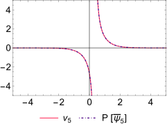
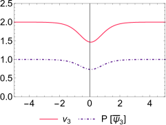
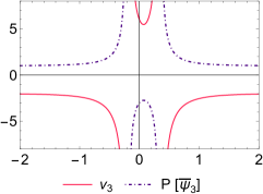
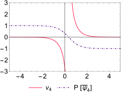
a) b) c) d) e)

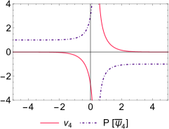
6.2 The smKdV-II (non-zero vacuum) solutions

Now, for the flows possessing a wider range of vacuums solutions, we can obtain novel combinations. First of all, for both positive and negative even flows, we must have a non-zero bosonic vacuum solution $(v_{0},\bar{\psi}_{0})=(v_{0},0)$ or $(v_{0},\bar{\psi}_{0})$. In that case, we can consider the vertex $V_{1}$, $V_{2}$ or $V_{3}$, leading to three different solutions:

$$v_{1} = v_{0},\qquad\bar{\psi}_{1}=\bar{\psi}_{0}+\left(\frac{4\bar{k}_{1}^{2}-v_{0}^{2}}{2\bar{k}_{1}}\right)c_{1}\bar{\psi}_{0}\rho_{N};$$ (6.19)

$$v_{2} = v_{0},\qquad\bar{\psi}_{2}=\left(\frac{4\bar{k}_{1}^{2}-v_{0}^{2}}{2\bar{k}_{1}}\right)\nu_{1}\rho_{N}.$$ (6.20)

where $\rho_{N}=\rho(x,t_{N})=e^{-2{k}_{1}x-\omega_{N}t_{N}}$, with eigenvalues given by

$$\omega_{3} = 2\bar{k}_{1}^{3}-\frac{3\bar{k}_{1}v_{0}^{2}}{2},\qquad\qquad\quad\,\,\,\,\qquad\qquad\mbox{for}\qquad N=3,$$ (6.21)

$$\omega_{-2} = \frac{4\bar{k}_{1}v_{0}^{2}\left(v_{0}-1\right)+16\bar{k}_{1}^{3}\left(v_{0}+1\right)}{v_{0}\left(4\bar{k}_{1}^{2}-v_{0}^{2}\right)^{2}},\qquad\mbox{for}\qquad N=-2,$$ (6.22)

Regarding $V_{3}(\bar{k}_{1})$, we have a more interesting solution that includes mixed terms

$$v_{3}=v_{0}+\partial_{x}\ln\left(\frac{1-\frac{\left(\bar{k}_{1}+v_{0}\right)}{2\bar{k}_{1}}\rho_{N}}{1+\frac{\left(\bar{k}_{1}-v_{0}\right)}{2\bar{k}_{1}}\rho_{N}}\right),\qquad\bar{\psi}_{3}=\bar{\psi}_{0}+\frac{\bar{\psi}_{0}}{v_{0}}\;\partial_{x}\ln\left(\frac{1-\frac{\left(\bar{k}_{1}+v_{0}\right)}{2\bar{k}_{1}}\rho_{N}}{1+\frac{\left(\bar{k}_{1}-v_{0}\right)}{2\bar{k}_{1}}\rho_{N}}\right),$$ (6.23)

with the eigenvalues

$$\omega_{3} = 2\bar{k}_{1}^{3}-3v_{0}^{2}\bar{k}_{1},\qquad\,\mbox{for}\qquad N=3,$$ (6.24)

$$\omega_{-2} = \frac{2\bar{k}_{1}}{v_{0}\left(\bar{k}_{1}^{2}-v_{0}^{2}\right)},\qquad\mbox{for}\qquad N=-2,$$ (6.25)

which can also be generalized using (6.9). In addition, we can also construct solutions for positive times with a different mixed vacuum $(v_{0},\bar{\psi}_{0})=(0,\bar{\psi}_{0})$, by using the vertices $V_{1}$ and $V_{4}$. We get

$$v_{1}=0,\qquad\bar{\psi}_{1}=\bar{\psi}_{0}+2{k}_{1}\bar{\psi}_{0}c_{1}\rho_{N},$$ (6.26)

and

$$v_{4}=\partial_{x}\ln\left(\frac{1-\frac{1}{2}\rho_{N}}{1+\frac{1}{2}\rho_{N}}\right),\qquad\bar{\psi}_{4}=\bar{\psi}_{0}+\frac{\left(2c_{1}\bar{\psi}_{0}+\bar{\psi}_{0}\rho_{N}\right)}{4\bar{k_{1}}}\partial_{x}\ln\left(\frac{1-\frac{1}{2}\rho_{N}}{1+\frac{1}{2}\rho_{N}}\right),$$ (6.27)

both with eigenvalue $\omega_{3}=2k_{1}^{3}$. In this case, we notice that $v_{0}$ does not contribute for the eigenvalue.

These results show us that introducing different parameters to the vacuum configuration leads to novel and interesting solutions that mix bosonic and fermionic parameters. The possibility of combining vacuum configurations lead us to six different solutions for smKdV-II models. In order to visualize the difference in the behavior of the solutions, in Figure 1 we have plotted the profile for the dynamical solutions $v_{3},\bar{\psi}_{3}$, $v_{4},\bar{\psi}_{4}$ and $v_{5},\bar{\psi}_{5}$. For the fermionic fields $\bar{\psi}_{i}$, we have plotted only the bosonic part of the solution, factorizing the Grassmann constant, namely the bosonic projection $P[\bar{\psi}_{i}]$, such that $\bar{\psi}_{i}=\bar{\psi}_{0}P[\bar{\psi}_{i}]$, or $\bar{\psi}_{i}=\nu_{1}P[\bar{\psi}_{i}]$. We see that different kind of solutions, kinks, anti-kinks, dark-solitons and peakons, appear by choosing the parameters accordingly.

In the next section, we will combine these solutions with the Gauge-super Miura transformation to obtain new solutions for the sKdV system.

7 The sKdV solutions via super Miura transformation

As highlighted in section 3, one can map the smKdV solutions into the sKdV solutions by using the super Miura transformation (3.6):

$$\begin{split}J&=v^{2}-\partial_{x}v+\bar{\psi}\partial_{x}\bar{\psi},\\ \bar{\chi}&=-v\bar{\psi}+\partial_{x}\bar{\psi}.\end{split}$$ (7.1)

Due the fact that the smKdV equation is invariant under the parity transformation $v\to-v$ and $\bar{\psi}\to-\bar{\psi}$, it is possible to obtain three other different kind of super Miura transformations, leading to four different possibilities. Here, we evaluate each one of them to obtain the corresponding sKdV solutions.

7.1 The sKdV-I (non-zero vacuum) solutions

For the sKdV-I hierarchy, we must have a zero vacuum solution such $(J_{0},\bar{\chi}_{0})=(0,0)$. In this case, we get six different solutions:

$$J_{2,-}^{\pm}=J_{2,+}^{\pm}=0,\qquad\chi_{2,-}^{\pm}=\chi_{2,+}^{\mp}=\pm 4{k}_{1}^{2}\nu_{1}\rho_{N},$$ (7.2)

and

$$J_{5,-}^{\pm}=-2\partial_{x}^{2}\ln\left(1-\frac{1}{2}\rho_{N}\right),\qquad\bar{\chi}_{5,-}^{\pm}=\pm 2\nu_{1}\;\partial_{x}^{2}\ln\left(1-\frac{1}{2}\rho_{N}\right),$$ (7.3)

$$J_{5,+}^{\pm}=-2\partial_{x}^{2}\ln\left(1+\frac{1}{2}\rho_{N}\right),\qquad\bar{\chi}_{5,-}^{\pm}=\pm 2\nu_{1}\;\partial_{x}^{2}\ln\left(1+\frac{1}{2}\rho_{N}\right),$$ (7.4)

with $\rho_{N}=\rho(x,t_{N})=e^{-2{k}_{1}x-\omega_{N}t_{N}}$.

(

(

(

(

(

(

Figure 2: Plots of the KdV-I and KdV-II solutions. We use both the positive and negative super Miura transformation for the bosonic field, and only the positive one for the fermionic field. (a-b) Using the zero vacuum solution $v_{5},\bar{\psi}_{5}$, we obtain two different solutions for sKdV. We obtain a peakon solution by using the first Miura, and by changing the SMiura leads to soliton/dark-soliton profile. (c) Now using the non-zero positive vacuum $v_{0}=2$, we obtain dark-solitons for the bosonic field and solitons for the fermionic projection for sKdV-II solutions. In such case, changing the super Miura only leads to a phase shift. (d) Setting a negative smKdV-II vacuum $v_{0}=-2$ leads to peakons solutions, although now the quadratic nature of the super Miura transformation leads to a positive vacuum for the sKdV-II field. (e - f) The $c_{1}$ dependent solution $v_{4},\bar{\psi}_{4}$ is quite interesting for the sKdV case. As the bosonic field does not depend on $c_{1}$, we have in both cases a peakon for the first super Miura, and dark-soliton for the second one. For the fermionic projection, in (e) the choice $c_{1}=-1$, leads to a null solution for the first Miura, and a dark-soliton for the second one. In turn, in (f) with the choice $c_{1}=1$, the first super Miura leads to a peakon solution, while the second one gives a solution that is always zero.

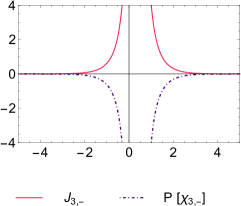
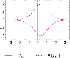
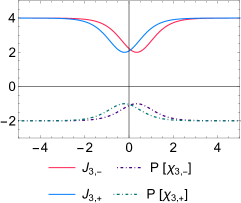
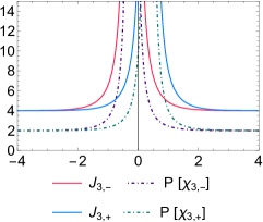
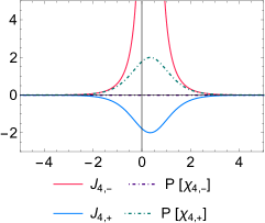
a) b) c) d) e) f)

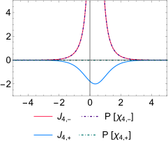
These solutions agree with the well-known format for KdV system, which includes a second-order derivative acting on the logarithmic term [54, 26]. Notice that the parity transformation for the bosonic field $v\to-v$ interchanges the $\tau_{0}$ function with the $\tau_{1}$ function. This features will be also present for a non-zero vacuum. On the other hand, the parity transformation for the fermionic field just changes a global sign.

7.2 The sKdV-II (non-zero vacuum) solutions

Now, for the sKdV-II flows, we find again several solutions associated to the different vacuum configurations. For $(J_{0},\bar{\chi}_{0})=(J_{0},0)$ or $(J_{0},\bar{\chi}_{0})$, we find twelve different solutions. The first set contains eight solutions where only the fermionic field is dynamical, namely

$$J_{1,-}^{\pm}=v_{0}^{2},\qquad\bar{\chi}_{1,-}^{\pm}=\mp v_{0}\bar{\psi}_{0}\mp\frac{\left(4\bar{k}_{1}^{2}-v_{0}^{2}\right)\left(v_{0}+2\bar{k}_{1}\right)}{2\bar{k}_{1}}c_{1}\bar{\psi}_{0}\rho_{N};$$ (7.5)

$$J_{1,+}^{\pm}=v_{0}^{2},\qquad\bar{\chi}_{1,+}^{\pm}=\mp v_{0}\bar{\psi}_{0}\mp\frac{\left(4\bar{k}_{1}^{2}-v_{0}^{2}\right)\left(v_{0}-2\bar{k}_{1}\right)}{2\bar{k}_{1}}c_{1}\bar{\psi}_{0}\rho_{N};$$ (7.6)

$$J_{2,-}^{\pm}=v_{0}^{2},\qquad\bar{\chi}_{2,-}^{\pm}=\mp\frac{\left(4\bar{k}_{1}^{2}-v_{0}^{2}\right)\left(v_{0}+2\bar{k}_{1}\right)}{2\bar{k}_{1}}\nu_{1}\rho_{N};$$ (7.7)

$$J_{2,+}^{\pm}=v_{0}^{2},\qquad\bar{\chi}_{2,+}^{\pm}=\mp\frac{\left(4\bar{k}_{1}^{2}-v_{0}^{2}\right)\left(v_{0}-2\bar{k}_{1}\right)}{2\bar{k}_{1}}\nu_{1}\rho_{N}.$$ (7.8)

Notice that the sKdV and smKdV vacuum is related by $J_{0}=v_{0}^{2}$, no matter if we are using the positive or negative sign for the bosonic field. Then, for the sKdV systems, the background for the bosonic vacuum is always positive. On the other hand, for the fermionic vacuum is $\chi_{0}=\pm v_{0}\bar{\psi}_{0}$, allowing both positive and negative configurations.

Finally, the remaining solutions contain both dynamical fields, but only a positive bosonic vacuum is possible. They have the following form,

$$J_{3,-}^{\pm}=v_{0}^{2}-2\partial_{x}^{2}\ln\Bigg(1-\frac{\left(v_{0}+\bar{k}_{1}\right)}{2\bar{k}_{1}}\rho_{N}\Bigg{missing}),\qquad\bar{\chi}_{3,-}^{\pm}=\mp v_{0}\bar{\psi}_{0}\;\pm\frac{2\bar{\psi}_{0}}{v_{0}}\partial_{x}^{2}\ln\Bigg(1-\frac{\left(v_{0}+\bar{k}_{1}\right)}{2\bar{k}_{1}}\rho_{N}\Bigg{missing})$$ (7.9)

$$J_{3,+}^{\pm}=v_{0}^{2}-2\partial_{x}^{2}\ln\Bigg(1+\frac{\left(\bar{k}_{1}-v_{0}\right)}{2\bar{k}_{1}}\rho_{N}\Bigg{missing}),\qquad\bar{\chi}_{3,+}^{\pm}=\mp v_{0}\bar{\psi}_{0}\;\pm\frac{2\bar{\psi}_{0}}{v_{0}}\partial_{x}^{2}\ln\left(1+\frac{\left(\bar{k}_{1}-v_{0}\right)}{2\bar{k}_{1}}\rho_{N}\right)$$ (7.10)

In addition, for the mixed vacuum configuration $(v_{0},\bar{\psi}_{0})=(0,\bar{\psi}_{0})$, we have

$$J_{1,-}^{\pm}=J_{1,+}^{\pm}=0,\qquad\bar{\chi}_{1,-}^{\pm}=\bar{\chi}_{1,+}^{\pm}=\pm 4{k}_{1}^{2}c_{1}\bar{\psi}_{0}\rho_{N},$$ (7.11)

and

$$J_{4,-}^{\pm}=-2\partial_{x}^{2}\ln\left(1-\frac{1}{2}\rho_{N}\right),\qquad\bar{\chi}_{4,-}^{\pm}=\pm\frac{\left(c_{1}+1\right)\bar{\psi}_{0}}{k_{1}}\;\partial_{x}^{2}\ln\left(1-\frac{1}{2}\rho_{N}\right);$$ (7.12)

$$J_{4,+}^{\pm}=-2\partial_{x}^{2}\ln\left(1+\frac{1}{2}\rho_{N}\right),\qquad\bar{\chi}_{4,-}^{\pm}=\pm\frac{\left(c_{1}-1\right)\bar{\psi}_{0}}{k_{1}}\;\partial_{x}^{2}\ln\left(1+\frac{1}{2}\rho_{N}\right).$$ (7.13)

An interesting feature about this solution is the possibility of having a vanishing fermionic solution for $\bar{\chi}_{4,-}$ if $c_{1}=-1$, or for $\bar{\chi}_{4,+}$ if $c_{1}=1$. In Figure 2, we have plotted the obtained solutions for skdV, where the upper index is always considered to be positive. Again, several interesting solutions appears, such as solitons, dark-solitons and peakons.

8 Discussion and further developments

In this paper we have extended the algebraic construction of positive flows to integrate the negative grade sector for both smKdV and sKdV hierarchies. These, follows the spirit developed for the pure bosonic case [49] with the inclusion of fermi fields.

The vacuum orbit plays a crucial role in classifying the hierarchies, splitting both smKdV and sKdV into two different types: the type-I hierarchy, which allows only a zero bosonic and fermionic vacuum, and a type-II hierarchy, which only have a non-zero bosonic vacuum. For the smKdV, the type I and II share the same positive flows but has different negative flows, while for the sKdV they share the same equations of motion for both the positive and negative part.

Soliton solutions for the smKdV were constructed by applying the dressing method. This approach generates different vacuum operators that form an abelian subalgebra, which is essential for the involution of the flows: $\left\{\mathcal{E}^{(2n+1)}\right\}$ for the smKdV-I, and $\left\{\Omega_{2m+1},\Gamma_{2m+1}\right\}$ for smKdV-II. Five different vertex operators were obtained in such context, leading to two different types of one-soliton solution for smKdV-I, and five solutions for smKdV-II.

Concerning the super Miura map, we have extend this transformation to all integer flows, whether they are positive or negative. For the negative flows, it was necessary to introduce an additional condition on the time derivatives of the sKdV field, the so-called temporal super Miura. These temporal relations are extremely important to show consistency of the gauge transformation for both super Miura and the dressing transformation, but also to prove the supersymmetry of $sKdV(-1)$. Another interesting result is the coalescence of two subsequent negative flows of smKdV hierarchy into a single flow of the sKdV. The soliton solutions for the sKdV hierarchy was obtained by using the super Miura transformation. Due to the existence of four possible super Miura transformation, we find that each smKdV solution lead to multiples solutions for sKdV.

On the other hand, regarding the vacuum structure, note that $\mathcal{E}^{(2n+1)}$ has degree $2n+1$ according the grading operator $\widehat{Q}\equiv 2\widehat{d}+\tfrac{1}{2}M_{1}^{(0)}$, whether $\Omega_{2m+1}$ and $\Gamma_{2m+1}$ would have different grades in each part of its components. This issue can be solved if we associate degree $1$ to $v_{0}$ and $\frac{1}{2}$ to $\bar{\psi}_{0}$, by redefining the grading operator as follows,

$$\widetilde{Q}\equiv\widehat{Q}+\widetilde{d}\quad\text{where}\quad\widetilde{d}\equiv v_{0}\tfrac{\partial}{\partial v_{0}}+\frac{1}{2}\bar{\psi}_{0}\tfrac{\partial}{\partial\bar{\psi}_{0}},$$ (8.1)

in such a way that both $\Omega_{2m+1}$ and $\Gamma_{2m+1}$ have degree $2n+1$, and the vacuums $v_{0},\;\bar{\psi}_{0}$ could be interpreted as the new spectral parameters. Thus, each term in $\mathcal{L}_{2n+1,\text{vac}}^{\text{smKdV}\text{-II}}$ and $\mathcal{L}_{-2n,\text{vac}}^{\text{smKdV}\text{-II}}$ has now grade $2n+1$ and $2n$, as would be expected. This idea had already been discussed previously in [49], but only $v_{0}$ was assumed to be a new spectral parameter, being possible to define a two-loop algebra [55] associated to it. In the supersymmetric case is necessary to introduce two new spectral parameters, making unclear whether this concept can be extended to a three-loop algebra. We intend to investigate this further.

In addition, it would be also interesting to explore different solutions with non-zero vacuum, such as multi-soliton solutions and quasi-periodic solutions in future investigations. The quasi-periodic solutions have already been obtained for supersymmetric systems by using different methods [56, 57], but we would like to extend the dressing method to obtain it more systematically. We also would like to implement the Bäcklund transformations [58] via a regular ansatz [28]. This will allow us to obtain the defect matrix for systems such as sKdV($-1$) and smKdV($-2$), and to use it for performing the scattering of the solutions. Finally, it would be also interesting to explore what would happen to the ZCC if we use a semi-integer ansatz for the Lax Pair, i.e. $N\in\mathbb{Z}+\frac{1}{2}$. Some of these issues are currently under investigations, and we hope to report it in the future.

Appendix

Appendix A The $sl(2,1)$ superalgebra

In this section, we present the algebraic structure used to construct the smKdV and sKdV integrable hierarchies. Let us consider super Kac-Moody algebra $\mathcal{G}=sl(2,1)$ generated by

$$L_{0} = \left\{h_{1}^{(m)}=\lambda^{m}h_{1},\;h_{2}^{(m)}=\lambda^{m}h_{2},\;E_{\pm\alpha_{1}}^{(m)}=\lambda^{m}E_{\pm\alpha_{1}},\hat{\kappa}\right\},$$

$$L_{1} = \left\{E_{\pm\alpha_{2}}^{(m)}=\lambda^{m}E_{\pm\alpha_{2}},\;E_{\pm(\alpha_{1}+\alpha_{2})}^{(m)}=\lambda^{m}E_{\pm(\alpha_{1}+\alpha_{2})}\right\},$$ (A.1)

where $\lambda\in\mathbb{C}$, $m\in\mathbb{N}$, $\hat{\kappa}$ is central extension term and

$$h_{1} = \left(\begin{matrix}1&0&0\\ 0&-1&0\\ 0&0&0\\ \end{matrix}\right),\quad h_{2}=\left(\begin{matrix}0&0&0\\ 0&1&0\\ 0&0&1\\ \end{matrix}\right),\quad E_{\alpha_{1}}=\left(\begin{matrix}0&1&0\\ 0&0&0\\ 0&0&0\\ \end{matrix}\right),\quad E_{-\alpha_{1}}=E_{\alpha_{1}}^{\dagger}$$

$$E_{\alpha_{2}} = \left(\begin{matrix}0&0&0\\ 0&0&1\\ 0&0&0\\ \end{matrix}\right),\quad E_{\alpha_{1}+\alpha_{2}}=\left(\begin{matrix}0&0&1\\ 0&0&0\\ 0&0&0\\ \end{matrix}\right),\quad E_{-\alpha_{2}}=E_{\alpha_{2}}^{\dagger},\quad E_{-(\alpha_{1}+\alpha_{2})}=E_{(\alpha_{1}+\alpha_{2})}^{\dagger}.\quad\mbox{}$$ (A.2)

The $L_{0}$ and $L_{1}$ are called the bosonic and fermionic parts of algebra, respectively, satisfying the following relations

$$\commutator{L_{0}}{L_{0}}\subset L_{0},\qquad\commutator{L_{0}}{L_{1}}\subset L_{1},\qquad\commutator{L_{1}}{L_{1}}\subset L_{0}.$$

The principal grading operator is defined by

$$Q=2\hat{d}+\frac{1}{2}h_{1},$$ (A.3)

where $\hat{d}$ is a derivation operator,

$$\commutator{\hat{d}}{T_{a}^{(m)}}=m\;T_{a}^{(m)},\quad\quad\quad T_{a}^{(m)}\in\mathcal{G}\,.$$

The principal grading operator decomposes the algebra in graded subspaces, $\mathcal{G}=\bigoplus_{a}\mathcal{G}_{a}$, where

$$\left[Q,\mathcal{G}_{a}\right]=a\;\mathcal{G}_{a},\qquad\left[\mathcal{G}_{a},\mathcal{G}_{b}\right]\in\mathcal{G}_{a+b},$$

for $a,b\in\mathbb{Z}$. For our purposes, the subspaces to consider are:

$$\begin{split}\mathcal{G}_{2m}&=\left\{h_{1}^{(m)}\right\},\\ \mathcal{G}_{2m+\frac{1}{2}}&=\left\{E_{\alpha_{2}}^{(m+\frac{1}{2})},\;E_{\alpha_{1}+\alpha_{2}}^{(m)},\;E_{-\alpha_{2}}^{(m)},\;E_{-\alpha_{1}-\alpha_{2}}^{(m+\frac{1}{2})}\right\},\\ \mathcal{G}_{2m+1}&=\left\{E_{\alpha_{1}}^{(m)},\;E_{-\alpha_{1}}^{(m+1)},\;h_{2}^{(m+\frac{1}{2})}\right\},\\ \mathcal{G}_{2m+\frac{3}{2}}&=\left\{E_{\alpha_{2}}^{(m+1)},\;E_{\alpha_{1}+\alpha_{2}}^{(m+\frac{1}{2})},\;E_{-\alpha_{2}}^{(m+\frac{1}{2})},\;E_{-\alpha_{1}-\alpha_{2}}^{(m+1)}\right\}.\end{split}$$ (A.4)

Another key ingredient in constructing our models is the grade one constant element, defined as

$$\mathcal{E}^{(1)}=E_{\alpha_{1}}^{(0)}+E_{-\alpha_{1}}^{(1)}+h_{1}^{(\frac{1}{2})}+2h_{2}^{(\frac{1}{2})}=\matrixquantity(\sqrt{\lambda}&1&0\\ \lambda&\sqrt{\lambda}&0\\ 0&0&2\sqrt{\lambda}),$$ (A.5)

which decomposes the algebra into $\mathcal{G}=\mathcal{K}\bigoplus\mathcal{M}$, where $\mathcal{K}_{\mathcal{E}}=\left\{x\in\mathcal{G}\,|\,\commutator{\mathcal{E}}{x}=0\right\}$ is the kernel of $\mathcal{E}$, and $\mathcal{M}_{\mathcal{E}}$ its complement,

$$\begin{split}\mathcal{K}_{\text{Bose}}=\mathcal{K}_{\mathcal{E}}\cap L_{0}&=\left\{K_{1}^{(2m+1},\;K_{2}^{(2m+1)}\right\},\\ \mathcal{K}_{\text{Fermi}}=\mathcal{K}_{\mathcal{E}}\cap L_{1}&=\left\{F_{1}^{(2m+\frac{1}{2})},\;F_{2}^{(2m+3/2)}\right\},\end{split}\quad\begin{split}\mathcal{M}_{\text{Bose}}=\mathcal{M}_{\mathcal{E}}\cap L_{0}&=\left\{M_{1}^{(2m)}\right\},\\ \mathcal{M}_{\text{Fermi}}=\mathcal{M}_{\mathcal{E}}\cap L_{1}&=\left\{G_{1}^{(2m+3/2)},\;G_{2}^{(2m+\frac{1}{2})}\right\}.\end{split}$$ (A.6)

The bosonic generators are be defined as

$$\begin{split}K_{1}^{(2m+1)}&=E_{\alpha_{1}}^{(m)}+E_{-\alpha_{1}}^{(m+1)},\\ K_{2}^{(2m+1)}&=h_{1}^{(m+\frac{1}{2})}+2h_{2}^{(m+\frac{1}{2})},\end{split}\qquad\begin{split}M_{1}^{(2m)}&=h_{1}^{(m)},\\ M_{2}^{(2m+1)}&=E_{\alpha_{1}}^{(m)}-E_{-\alpha_{1}}^{(m+1)},\end{split}$$

and the fermionic generators are

$$F_{1}^{(2m+\frac{1}{2})} =\left(E_{\alpha_{2}}^{(m+\frac{1}{2})}+E_{\alpha_{1}+\alpha_{2}}^{(m)}\right)+\left(E_{-\alpha_{2}}^{(m)}+E_{-\left(\alpha_{1}+\alpha_{2}\right)}^{(m+\frac{1}{2})}\right),$$

$$F_{2}^{(2m+\frac{3}{2})} =\left(E_{\alpha_{2}}^{(m+1)}+E_{\alpha_{1}+\alpha_{2}}^{(m+\frac{1}{2})}\right)-\left(E_{-\alpha_{2}}^{(m+\frac{1}{2})}+E_{-\left(\alpha_{1}+\alpha_{2}\right)}^{(m+1)}\right),$$

$$G_{1}^{(2m+\frac{3}{2})} =\left(E_{\alpha_{2}}^{(m+1)}-E_{\alpha_{1}+\alpha_{2}}^{(m+\frac{1}{2})}\right)+\left(E_{-\alpha_{2}}^{(m+\frac{1}{2})}-E_{-\left(\alpha_{1}+\alpha_{2}\right)}^{(m+1)}\right),$$

$$G_{2}^{(2m+\frac{1}{2})} =\left(E_{\alpha_{2}}^{(m+\frac{1}{2})}-E_{\alpha_{1}+\alpha_{2}}^{(m)}\right)-\left(E_{-\alpha_{2}}^{(m)}-E_{-\left(\alpha_{1}+\alpha_{2}\right)}^{(m+\frac{1}{2})}\right).$$

From (A.3) and (A.5), we can reorganize the graded subspaces (A.4) in terms of the kernel-image decomposition in the following way,

$$\begin{split}\mathcal{G}_{2m}&=\left\{M_{1}^{(2m)}\right\},\\ \mathcal{G}_{2m+\frac{1}{2}}&=\left\{F_{1}^{(2m+\frac{1}{2})},\;G_{2}^{(2m+\frac{1}{2})}\right\},\\ \mathcal{G}_{2m+1}&=\left\{K_{1}^{(2m+1)},\;K_{2}^{(2m+1)},\;M_{2}^{(2m+1)}\right\},\\ \mathcal{G}_{2m+\frac{3}{2}}&=\left\{F_{2}^{(2m+\frac{3}{2})},\;G_{1}^{(2m+\frac{3}{2})}\right\}.\end{split}$$ (A.8)

The commutation relations of the algebra are then given by

$$\begin{split}&\commutator{K_{1}^{(2m+1)}}{K_{1}^{(2n+1)}}=\hat{\kappa}(m-n)\delta_{n+m+1,0},\\ &\commutator{K_{1}^{(2m+1)}}{K_{2}^{(2n+1)}}=0,\\ &\commutator{K_{1}^{(2m+1)}}{M_{1}^{(2n)}}=-2M_{2}^{(2m+2n+1)},\\ &\commutator{K_{1}^{(2m+1)}}{M_{2}^{(2n+1)}}=-2M_{1}^{(2(m+n+1))}-\hat{\kappa}(m+n)\delta_{n+m+1,0},\\ &\commutator{K_{2}^{(2m+1)}}{K_{2}^{(2n+1)}}=-\hat{\kappa}(2m+1)\delta_{n+m+1,0},\\ &\commutator{K_{2}^{(2m+1)}}{M_{1}^{(2n)}}=0,\\ &\commutator{K_{2}^{(2m+1)}}{M_{2}^{(2n+1)}}=0,\\ &\commutator{M_{1}^{(2m)}}{M_{1}^{(2n)}}=2\hat{\kappa}m\delta_{m+n,0},\\ &\commutator{M_{1}^{(2m)}}{M_{2}^{(2n+1)}}=2K_{1}^{(2m+2n+1)},\\ &\commutator{M_{2}^{(2m+1)}}{M_{2}^{(2n+1)}}=-\hat{\kappa}(m-n)\delta_{n+m+1,0},\\ &\commutator{K_{1}^{(2m+1)}}{F_{1}^{(2n+1/2)}}=F_{2}^{(2(m+n)+3/2)},\\ &\commutator{K_{1}^{(2m+1)}}{F_{2}^{(2n+3/2)}}=F_{1}^{(2(m+n+1)+1/2)},\\ &\commutator{K_{1}^{(2m+1)}}{G_{1}^{(2n+3/2)}}=-G_{2}^{(2(m+n+1)+1/2)},\end{split}\begin{split}&\commutator{K_{1}^{(2m+1)}}{G_{2}^{(2n+1/2)}}=-G_{1}^{(2(m+n)+3/2)},\\ &\commutator{K_{2}^{(2m+1)}}{F_{1}^{(2n+1/2)}}=-F_{2}^{(2(m+n)+3/2)},\\ &\commutator{K_{2}^{(2m+1)}}{F_{2}^{(2n+3/2)}}=-F_{1}^{(2(m+n+1)+1/2)},\\ &\commutator{K_{2}^{(2m+1)}}{G_{1}^{(2n+3/2)}}=-G_{2}^{(2(m+n+1)+1/2)},\\ &\commutator{K_{2}^{(2m+1)}}{G_{2}^{(2n+1/2)}}=-G_{1}^{(2(m+n)+3/2)},\\ &\commutator{M_{1}^{(2m)}}{F_{1}^{(2n+1/2)}}=-G_{2}^{(2(m+2)+1/2)},\\ &\commutator{M_{1}^{(2m)}}{F_{2}^{(2n+3/2)}}=-G_{1}^{(2(m+2)+3/2)},\\ &\commutator{M_{1}^{(2m)}}{G_{1}^{(2n+3/2)}}=-F_{2}^{(2(m+2)+3/2)},\\ &\commutator{M_{1}^{(2m+1)}}{G_{2}^{(2n+1/2)}}=-F_{1}^{(2(m+2)+1/2)},\\ &\commutator{M_{2}^{(2m+1)}}{F_{1}^{(2n+1/2)}}=-G_{1}^{(2(m+n)+3/2)},\\ &\commutator{M_{2}^{(2m+1)}}{F_{2}^{(2n+3/2)}}=-G_{2}^{(2(m+n+1)+1/2)},\\ &\commutator{M_{2}^{(2m+1)}}{G_{1}^{(2n+3/2)}}=F_{1}^{(2(m+n+1)+1/2)},\\ &\commutator{M_{2}^{(2m+1)}}{G_{2}^{(2n+1/2)}}=F_{2}^{(2(m+n)+3/2)}.\end{split}$$

and the anti-commutations relations, given by

$$\begin{split}\anticommutator{F_{1}^{(2m+1/2)}}{F_{1}^{(2n+1/2)}}&=2(K_{1}^{(2m+2n+1)}+K_{2}^{(2m+2n+1)})-\hat{\kappa}(4m+1)\delta_{n+m+1,0},\\ \anticommutator{F_{1}^{(2m+1/2)}}{F_{2}^{(2n+3/2)}}&=0,\\ \anticommutator{F_{1}^{(2m+1/2)}}{G_{1}^{(2n+3/2)}}&=-2M_{1}^{(2(m+n+1))}+\hat{\kappa}\delta_{n+m+1,0},\\ \anticommutator{F_{1}^{(2m+1/2)}}{G_{2}^{(2n+1/2)}}&=-2M_{2}^{(2m+2n+1)},\\ \anticommutator{F_{2}^{(2m+3/2)}}{F_{2}^{(2n+3/2)}}&=-(K_{1}^{(2(m+n+1)+1)}+K_{2}^{(2(m+n+1)+1)}),\\ \anticommutator{F_{2}^{(2m+3/2)}}{G_{1}^{(2n+3/2)}}&=2M_{2}^{(2(m+n+1)+1)},\\ \anticommutator{F_{2}^{(2m+3/2)}}{G_{2}^{(2n+1/2)}}&=2M_{1}^{(2(m+n+1))}-\hat{\kappa}\delta_{n+m+1,0},\\ \anticommutator{G_{1}^{(2m+3/2)}}{G_{1}^{(2n+3/2)}}&=-2(K_{1}^{(2(m+n+1)+1)}-K_{2}^{(2(m+n+1)+1)}),\\ \anticommutator{G_{1}^{(2m+3/2)}}{G_{2}^{(2n+1/2)}}&=\hat{\kappa}\left(2m-2n-1\right)\delta_{n+m+1,0},\\ \anticommutator{G_{2}^{(2m+1/2)}}{G_{2}^{(2n+1/2)}}&=2(K_{1}^{(2m+2n+1)}+K_{2}^{(2m+2n+1)}).\end{split}$$

Appendix B Grade decomposition of zero curvature condition

In this appendix, we present explicitly the grade by grade decomposition proposed for each ansatz in section 2.

• The smKdV positive flows

  $$\commutator{\partial_{x}+A_{x}}{\;\partial_{t_{N}}+D^{(N)}_{N}+D^{(N-\frac{1}{2})}_{N}+\cdots+D^{(0)}_{N}}=0,$$ (B.1)

  decomposes as follows

  $$\commutator{{\mathcal{E}}^{(1)}}{D^{(N)}_{N}} =0,$$ (B.2a)

  $$\commutator{{\mathcal{E}}^{(1)}}{D^{(N-\frac{1}{2})}_{N}}+\commutator{A_{\frac{1}{2}}}{D^{(N)}_{N}} =0,$$ (B.2b)

  $$\commutator{{\mathcal{E}}^{(1)}}{D^{(N-1)}_{N}}+\commutator{A_{\frac{1}{2}}}{D^{(N-\frac{1}{2})}_{N}}+\commutator{A_{0}}{D^{(N)}_{N}}+\partial_{x}D^{(N)}_{N} =0,$$ (B.2c)

  $$\;\;\vdots$$

  $$\commutator{A_{\frac{1}{2}}}{D^{(0)}_{N}}+\commutator{A_{0}}{D^{(\frac{1}{2})}_{N}}+\partial_{x}D^{(\frac{1}{2})}_{N}-\partial_{t_{N}}A_{\frac{1}{2}} =0,$$ (B.2d)

  $$\commutator{A_{0}}{D^{(0)}_{N}}+\partial_{x}D^{(0)}_{N}-\partial_{t_{N}}A_{0} =0$$ (B.2e)

• For sKdV positive flows, we have

  $$\commutator{\partial_{x}+A_{x}}{\;\partial_{t_{N}}+\mathcal{D}^{(N)}_{N}+\mathcal{D}^{(N-\frac{1}{2})}_{N}+\cdots+\mathcal{D}^{(-1)}_{N}}=0,$$ (B.3)

  $$\commutator{{\mathcal{E}}^{(1)}}{\mathcal{D}^{(N)}_{N}} =0,$$ (B.4a)

  $$\commutator{{\mathcal{E}}^{(1)}}{\mathcal{D}^{(N-\frac{1}{2})}_{N}} =0,$$ (B.4b)

  $$\partial_{x}\mathcal{D}^{(N)}_{N}+\commutator{{\mathcal{E}}^{(1)}}{\mathcal{D}^{(N-1)}_{N}} =0,$$ (B.4c)

  $$\;\;\vdots$$

  $$\partial_{x}\mathcal{D}^{(-\frac{1}{2})}_{N}+\commutator{A_{-1}}{\mathcal{D}^{(\frac{1}{2})}_{N}}+\commutator{A_{-\frac{1}{2}}}{\mathcal{D}^{(0)}_{N}}-\partial_{t_{N}}A_{-\frac{1}{2}} =0,$$ (B.4d)

  $$\partial_{x}\mathcal{D}^{(-1)}_{N}+\commutator{A_{-1}}{\mathcal{D}^{(0)}_{N}}+\commutator{A_{-\frac{1}{2}}}{\mathcal{D}^{(-\frac{1}{2})}_{N}}-\partial_{t_{N}}A_{-1} =0.$$ (B.4e)

• The smKdV negative flows

  $$\commutator{\partial_{x}+A_{x}}{\;\partial_{t_{-N}}+D^{(-\frac{1}{2})}_{-N}+D^{(-1)}_{N}+\cdots+D^{(-N)}_{-N}}=0,$$ (B.5)

  decomposes as follows

  $$\commutator{A_{0}}{D^{(-N)}_{-N}}+\partial_{x}D^{(-N)}_{-N} =0,$$ (B.6a)

  $$\commutator{A_{\frac{1}{2}}}{D^{(-N)}_{-N}}+\commutator{A_{0}}{D^{(-N+\frac{1}{2})}_{-N}}+\partial_{x}D^{(-N+\frac{1}{2})}_{-N} =0,$$ (B.6b)

  $$\;\;\vdots$$

  $$\commutator{{\mathcal{E}}^{(1)}}{D^{(-1)}_{-N}}+\commutator{A_{0}}{D^{(-\frac{1}{2})}_{-N}}-\partial_{t_{-N}}A_{0} =0,$$ (B.6c)

  $$\commutator{{\mathcal{E}}^{(1)}}{D^{(-\frac{1}{2})}_{-N}}-\partial_{t_{-N}}A_{\frac{1}{2}} =0.$$ (B.6d)

• The sKdV negative flows

  $$\commutator{\partial_{x}+A_{x}}{\;\partial_{t_{-N}}+\mathcal{D}^{(-\frac{1}{2})}_{-N}+\mathcal{D}^{(-1)}_{N}+\cdots+\mathcal{D}^{(-N-2)}_{-N}}=0,$$ (B.7)

  decomposes in the following way

  $$\commutator{A_{-1}}{\mathcal{D}^{(-N-2)}_{-N}} =0,$$ (B.8a)

  $$\commutator{A_{-\frac{1}{2}}}{\mathcal{D}^{(-N-2)}_{-N}}+\commutator{A_{-1}}{\mathcal{D}^{(-N-\frac{3}{2})}_{-N}} =0,$$ (B.8b)

  $$\partial_{x}\mathcal{D}^{(-N-2)}_{-N}+\commutator{A_{-1}}{\mathcal{D}^{(-N-1)}_{-N}}+\commutator{A_{-\frac{1}{2}}}{\mathcal{D}^{(-N-\frac{3}{2})}_{-N}} =0,$$ (B.8c)

  $$\;\;\vdots$$

  $$\partial_{x}\mathcal{D}^{(-1)}_{-N}+\commutator{A_{-\frac{1}{2}}}{\mathcal{D}^{(-\frac{1}{2})}_{-N}}+\commutator{{\mathcal{E}}^{(1)}}{\mathcal{D}^{(-2)}_{-N}}-\partial_{t_{-N}}A_{-1} =0,$$ (B.8d)

  $$\partial_{x}\mathcal{D}^{(-\frac{1}{2})}_{-N}+\commutator{{\mathcal{E}}^{(1)}}{\mathcal{D}^{(-\frac{3}{2})}_{-N}}-\partial_{t_{-N}}A_{-\frac{1}{2}} =0,$$ (B.8e)

  $$\commutator{{\mathcal{E}}^{(1)}}{\mathcal{D}^{(-1)}_{-N}} =0,$$ (B.8f)

  $$\commutator{{\mathcal{E}}^{(1)}}{\mathcal{D}^{(-\frac{1}{2})}_{-N}} =0.$$ (B.8g)

Appendix C Lax Pairs for smKdV and sKdV

Here we present the explicit form of the Lax pairs for some specific flows of both sKdV and smKdV hierarchies.

C.1 The smKdV hierarchy

• $N=3$

  $$\begin{split}A_{t_{3}}^{\text{smKdV}}=&\;\;K_{1}^{(3)}+K_{2}^{(3)}+\bar{\psi}\;G_{2}^{(\frac{5}{2})}+v\;M_{1}^{(2)}+\frac{1}{2}v\;\bar{\psi}\;F_{2}^{(\frac{3}{2})}+\frac{1}{2}\partial_{x}\bar{\psi}\;G_{1}^{(\frac{3}{2})}\\ &-\frac{1}{2}\left\{v^{2}+\bar{\psi}\partial_{x}\bar{\psi}\right\}K_{1}^{(1)}+\frac{1}{2}\bar{\psi}\partial_{x}\bar{\psi}\;K_{2}^{(1)}+\frac{1}{2}\partial_{x}v\;M_{2}^{(1)}\\ &+\frac{1}{4}\left\{v\partial_{x}\bar{\psi}-\partial_{x}v\bar{\psi}\right\}\;F_{1}^{(\frac{1}{2})}+\left\{\frac{1}{4}\partial_{x}^{2}\bar{\psi}-\frac{1}{2}v^{2}\bar{\psi}\right\}\;G_{2}^{\frac{1}{2}}\\ &+\left\{\frac{1}{4}\partial_{x}^{2}v-\frac{1}{2}v^{3}-\frac{3}{4}v\bar{\psi}\partial_{x}\bar{\psi}\right\}\;M_{1}^{(0)}\end{split}$$ (C.1)

• $N=5$

  $$A^{\text{smKdV}}_{t_{5}}=D^{(5)}_{5}+D^{(\frac{9}{2})}_{5}+\cdots+D^{(0)}_{5}$$ (C.2)

  with

  $$D^{(5)}_{5} =K_{1}^{(5)}+K_{2}^{(5)}=\mathcal{E}^{(5)},$$

  $$D^{(\frac{9}{2})}_{5} =\bar{\psi}\;G_{2}^{(9/2)},$$

  $$D^{(4)}_{5} =v\;M_{1}^{(4)},$$

  $$D^{(\frac{7}{2})}_{5} =\frac{1}{2}v\bar{\psi}\;F_{2}^{(7/2)}+\frac{1}{2}\partial_{x}\bar{\psi}\;G_{1}^{(7/2)},$$

  $$D^{(3)}_{5} =-\frac{1}{2}\left(\bar{\psi}\partial_{x}\bar{\psi}+v^{2}\right)\;K_{1}^{(3)}+\frac{1}{2}\bar{\psi}\partial_{x}\bar{\psi}\;K_{2}^{(3)}+\frac{1}{2}\partial_{x}v\;M_{2}^{(3)},$$

  $$D^{(\frac{5}{2})}_{5} =\frac{1}{4}\left(v\partial_{x}\bar{-}\partial_{x}v\bar{\psi}\right)F_{1}^{(5/2)}+\frac{1}{4}\left(-2v^{2}\bar{\psi}+\partial_{x}^{2}\bar{\psi}\right)\;G_{2}^{(5/2)},$$

  $$D^{(2)}_{5} =\frac{1}{4}\left(-3v\bar{\psi}\partial_{x}\bar{\psi}-2v^{3}+\partial_{x}^{2}v\right)\;M_{1}^{(2)},$$

  $$D^{(\frac{3}{2})}_{5} =\frac{1}{8}\left(v\partial_{x}^{2}\bar{\psi}+\bar{\psi}\partial_{x}^{2}v-v^{3}\bar{\psi}-\partial_{x}v\partial_{x}\bar{\psi}\right)\;F_{2}^{(3/2)}+\frac{1}{8}\left(\partial_{x}^{3}\bar{\psi}-3v^{2}\partial_{x}\bar{\psi}-3v\partial_{x}v\bar{\psi}\right)\;G_{1}^{(3/2)},$$

  $$D^{(1)}_{5} =\frac{1}{8}\left(\bar{\psi}\partial_{x}^{3}\bar{\psi}-\partial_{x}\bar{\psi}\partial_{x}^{2}\bar{\psi}-8v^{2}\bar{\psi}\partial_{x}\bar{\psi}-(\partial_{x}v)^{2}+2v\partial_{x}^{2}v-3v^{4}\right)\;K_{1}^{(1)}$$

  $$+\frac{1}{8}\left(\bar{\psi}\partial_{x}^{3}\bar{\psi}-\partial_{x}\bar{\psi}\partial_{x}^{2}\bar{\psi}-4v^{2}\bar{\psi}\partial_{x}\bar{\psi}\right)\;K_{2}^{(1)}+\frac{1}{8}\left(\partial_{x}^{3}v-6v^{2}\partial_{x}v-4\partial_{x}v\bar{\psi}\partial_{x}\bar{\psi}-2v\bar{\psi}\partial_{x}^{2}\bar{\psi}\right)\;M_{2}^{(1)},$$

  $$D^{(\frac{1}{2})}_{5} =\frac{1}{16}\left(4v^{2}\partial_{x}v\bar{\psi}-4v^{3}\partial_{x}\bar{\psi}-\partial_{x}v\partial_{x}^{2}\bar{\psi}+\partial_{x}^{2}v\partial_{x}\bar{\psi}+v\partial_{x}^{3}\bar{\psi}-\partial_{x}^{3}v\bar{\psi}\right)\;F_{1}^{(1/2)}$$

  $$+\frac{1}{16}\left(\partial_{x}^{4}\bar{\psi}-4v^{2}\partial_{x}^{2}\bar{\psi}-8v\partial_{x}v\partial_{x}\bar{\psi}-2(\partial_{x}v)^{2}\bar{\psi}-6v\partial_{x}^{2}v\bar{\psi}+6v^{4}\bar{\psi}\right)\;G_{2}^{(1/2)},$$

  $$D^{(0)}_{5} =\frac{1}{16}\left(\partial_{x}^{4}v-10v^{2}\partial_{x}^{2}v-10v(\partial_{x}v)^{2}+6v^{5}+20v^{3}\bar{\psi}\partial_{x}\bar{\psi}-5\partial_{x}(\partial_{x}v\bar{\psi}\partial_{x}\bar{\psi})-5v\bar{\psi}\partial_{x}^{3}\bar{\psi}\right)M_{1}^{(2)}.$$

• $N=\frac{1}{2}$

  $$A_{t_{\frac{1}{2}}}^{\text{smKdV}}=\xi F_{1}^{(\frac{1}{2})}+\xi\bar{\psi}M_{1}^{(0)}$$ (C.4)

• $N=-1$

  $$A_{t_{-1}}^{\text{smKdV}}=\cosh{2\phi}\;K_{1}^{(-1)}+K_{2}^{(-1)}-\sinh{2\phi}\;M_{2}^{(-1)}-\psi\sinh{\phi}\;F_{2}^{(-\frac{1}{2})}-\psi\cosh{\phi}\;G_{1}^{(-\frac{1}{2})}$$ (C.5)

  where $v(x,t_{-1})=\partial_{x}\phi(x,t_{-1})$.

• $N=-2$

  $$A_{t_{-2}}^{\text{smKdV}} =M_{1}^{(-2)}-\frac{e^{\phi}\psi_{-}}{2}\left(F_{1}^{(-\frac{3}{2})}+G_{2}^{(-\frac{3}{2})}\right)-\frac{e^{-\phi}\psi_{+}}{2}\left(F_{1}^{(-\frac{3}{2})}-G_{2}^{(-\frac{3}{2})}\right)$$

  $$+a_{-}\left(K_{1}^{(-1)}+M_{2}^{(-1)}\right)-a_{+}\left(K_{1}^{(-1)}-M_{2}^{(-1)}\right)+\left(1+\psi_{-}\psi_{+}\right)K_{2}^{(-1)}$$ (C.6)

  $$+\Omega_{+}\left(F_{2}^{(-\frac{1}{2})}+G_{1}^{(-\frac{1}{2})}\right)+\Omega_{-}\left(F_{2}^{(-\frac{1}{2})}-G_{1}^{(-\frac{1}{2})}\right)$$

  where

  $$v=\partial_{x}\phi\quad\quad\psi_{\pm}=\partial_{x}^{-1}\left(e^{\pm\phi}\bar{\psi}\right),\quad\quad a_{\pm}=e^{\pm 2\phi}\partial_{x}^{-1}\left[e^{\mp 2\phi}\left(1+\psi_{\mp}\partial_{x}\psi_{\pm}\right)\right],$$

  and

  $$\Omega_{\pm}=\frac{e^{\pm\phi}}{2}\partial_{x}^{-1}\left[e^{\mp 2\phi}\psi_{\pm}-\psi_{\mp}\mp\partial_{x}\psi_{\mp}\left(1+\psi_{-}\psi_{+}\mp 2a_{\pm}\right)\right].$$

C.2 The sKdV hierarchy

• $N=3$

  $$\begin{split}A_{t_{3}}^{\text{sKdV}}=&\;\;K_{1}^{(3)}+K_{2}^{(3)}+\frac{\bar{\chi}}{2}G_{1}^{\left(\frac{3}{2}\right)}-\frac{J}{2}M_{2}^{(1)}+\frac{\partial_{x}\bar{\chi}}{4}G_{2}^{\left(\frac{1}{2}\right)}\\ &-\frac{\partial_{x}J}{4}M_{1}^{(0)}+\left(\frac{\partial_{x}^{2}\chi}{8}-\frac{J\bar{\chi}}{4}\right)\left(G_{1}^{\left(\frac{2}{2}\right)}+F_{2}^{\left(-\frac{1}{2}\right)}\right)\\ &+\left(\frac{\partial_{x}^{2}J}{8}-\frac{J^{2}}{4}-\frac{\bar{\chi}\partial_{x}\bar{\chi}}{8}\right)\left(K_{1}^{(-1)}-M_{2}^{(-1)}\right)\end{split}$$ (C.7)

• $N=5$

  $$A^{\text{sKdV}}_{t_{5}}=\mathcal{D}^{(5)}_{5}+\mathcal{D}^{(\frac{9}{2})}_{5}+\cdots+\mathcal{D}^{(-1)}_{5}$$ (C.8)

  with

  $$\mathcal{D}^{(5)}_{5} =K_{1}^{(5)}+K_{2}^{(5)}=\mathcal{E}^{(5)},$$

  $$\mathcal{D}^{(\frac{9}{2})}_{5} =0,$$

  $$\mathcal{D}^{(4)}_{5} =0,$$

  $$\mathcal{D}^{(\frac{7}{2})}_{5} =\frac{\bar{\chi}}{2}G_{1}^{(\frac{7}{2})}$$

  $$\mathcal{D}^{(3)}_{5} =-\frac{J}{2}M_{2}^{(3)},$$

  $$\mathcal{D}^{(\frac{5}{2})}_{5} =\frac{\partial_{x}\bar{\chi}}{4}G_{2}^{(\frac{5}{2})}$$

  $$\mathcal{D}^{(2)}_{5} =-\frac{\partial_{x}J}{4}M_{1}^{(2)},$$

  $$\mathcal{D}^{(\frac{3}{2})}_{5} =\frac{J\bar{\chi}}{8}F_{2}^{(\frac{3}{2})}+\frac{1}{8}\left(\partial_{x}^{2}\bar{\chi}-2J\bar{\chi}\right)G_{1}^{(\frac{3}{2})},$$

  $$\mathcal{D}^{(1)}_{5} =\frac{1}{8}\left(J^{2}+\bar{\chi}\partial_{x}\bar{\chi}\right)K_{1}^{(1)}-\frac{1}{8}\bar{\chi}\partial_{x}\bar{\chi}K_{2}^{(1)}+\frac{1}{8}\left(-\partial_{x}^{2}J+2J^{2}+\bar{\chi}\partial_{x}\bar{\chi}\right)M_{2}^{(1)},$$

  $$\mathcal{D}^{(\frac{1}{2})}_{5} =\frac{1}{16}\left(-\partial_{x}J\bar{\chi}+J\partial_{x}\bar{\chi}\right)F_{1}^{(\frac{1}{2})}+\frac{1}{16}\left(-\partial_{x}^{3}\bar{\chi}-3\partial_{x}\left(J\bar{\chi}\right)\right)G_{2}^{(\frac{1}{2})},$$

  $$\mathcal{D}^{(0)}_{5} =\frac{1}{16}\left(-\partial_{x}^{3}J+3\partial_{x}J^{2}+2\bar{\chi}\partial_{x}^{2}\bar{\chi}\right)M_{1}^{(0)},$$

  $$\mathcal{D}^{(-\frac{1}{2})}_{5} =\frac{1}{32}\left(\partial_{x}^{4}\bar{\chi}-3\partial_{x}^{2}(J\bar{\chi})+6J^{2}\bar{\chi}-J\partial_{x}^{2}\bar{\chi}-\partial_{x}^{2}J\bar{\chi}\right)\left(F_{2}^{(-\frac{1}{2})}+G_{1}^{(-\frac{1}{2})}\right),$$

  $$\mathcal{D}^{(-1)}_{5} =\frac{1}{32}\left(\partial_{x}^{4}J-6(\partial_{x}J)^{2}-8J\partial_{x}^{2}J+6J^{3}-4\bar{\chi}\partial_{x}^{3}\bar{\chi}+8J\bar{\chi}\partial_{x}\bar{\chi}\right)\left(K_{1}^{(-1)}-M_{2}^{(-1)}\right).$$

• $N=\frac{1}{2}$

  $$A_{t_{\frac{1}{2}}}^{\text{sKdV}}=\xi F_{1}^{(\frac{1}{2})}-\xi\bar{\chi}\left(K_{1}^{(-1)}-M_{2}^{(-1)}\right)$$ (C.10)

• $N=-1$

  $$A^{\text{sKdV}}_{t_{-1}}=\mathcal{D}^{(-3)}_{-1}+\mathcal{D}^{(-\frac{5}{2})}_{-1}+\cdots+\mathcal{D}^{(-\frac{1}{2})}_{-1}$$ (C.11)

  with

  $$\mathcal{D}^{{(-3)}}_{-1} =-\frac{1}{8}\left\{\partial_{x}(\partial_{t_{-1}}\partial_{x}\eta+\partial_{x}\gamma)-2\partial_{x}\eta\left(\partial_{t_{-1}}\eta+\gamma\right)\right.$$

  $$\qquad\qquad\qquad\left.+\partial_{x}\bar{\eta}\left(\bar{\nu}_{-}-\bar{\nu}_{+}+2\bar{\gamma}-\partial_{t_{-1}}\partial_{x}\bar{\gamma}\right)\right\}\left(K_{1}^{(-3)}-M_{2}^{(-3)}\right),$$

  $$\mathcal{D}^{(-\frac{5}{2})}_{-1} =\frac{1}{8}\left(\partial_{x}(\bar{\nu}_{+}+\bar{\nu}_{-})-\partial_{t_{-1}}\partial_{x}^{2}\bar{\gamma}+2\partial_{x}\bar{\gamma}\;\gamma+2\partial_{x}\bar{\gamma}\right)\left(F_{2}^{(-\frac{5}{2})}+G_{1}^{(-\frac{5}{2})}\right),$$

  $$\mathcal{D}^{(-2)}_{-1} =\frac{1}{4}\left(\partial_{t_{-1}}\partial_{x}\eta+\partial_{x}\gamma\right)\;M_{1}^{(-2)},$$

  $$\mathcal{D}^{(-\frac{3}{2})}_{-1} =\frac{1}{4}\left(\bar{\nu}_{+}-\bar{\nu}_{-}-2\bar{\gamma}\right)\;F_{1}^{(-\frac{3}{2})}-\frac{1}{4}\partial_{t_{-1}}\partial_{x}\bar{\gamma}\;G_{2}^{(-\frac{3}{2})},$$

  $$\mathcal{D}^{(-1)}_{-1} =\frac{1}{2}\gamma\left(K_{1}^{(-1)}+K_{2}^{(-1)}\right)+\frac{1}{2}\partial_{t_{-1}}\eta\;K_{1}^{(-1)}+K_{2}^{(-1)},$$

  $$\mathcal{D}^{(-\frac{1}{2})}_{-1} =\frac{1}{2}\partial_{t_{-1}}\bar{\gamma}\;F_{2}^{(-\frac{1}{2})}.$$

Appendix D Supersymmetry transformation for smKdV$(-2)$

Let us consider the field equations for $smKdV(-2)$,

$$\partial_{t_{-2}}\partial_{x}\phi =-2\left(a_{-}+a_{+}\right)+2\bar{\psi}\left(\Omega_{-}+\Omega_{+}\right),$$ (D.1a)

$$\partial_{t_{-2}}\bar{\psi} =-2\left(\Omega_{+}-\Omega_{-}\right),$$ (D.1b)

with

$$\psi_{\pm} =\partial_{x}^{-1}\left(e^{\pm\phi}\bar{\psi}\right),$$ (D.2a)

$$a_{\pm} =e^{\pm 2\phi}\partial_{x}^{-1}\left[e^{\mp 2\phi}\left(1+\psi_{\mp}\partial_{x}\psi_{\pm}\right)\right],$$ (D.2b)

and

$$\Omega_{\pm}=\frac{e^{\pm\phi}}{2}\partial_{x}^{-1}\left[e^{\mp 2\phi}\psi_{\pm}-\psi_{\mp}\mp\left(\partial_{x}\psi_{\mp}\right)\left(1+\psi_{-}\psi_{+}\mp 2a_{\pm}\right)\right],$$ (D.3)

where the anti-derivative operator is defined by $\partial_{x}^{-1}f=\int^{x}f(y)\differential{y}$. By applying the supersymmetry transformation

$$\delta v =\xi\;\partial_{x}\bar{\psi}\quad\to\quad\delta\phi=\xi\bar{\psi},$$ (D.4a)

$$\delta\bar{\psi} =-\xi\;v=-\xi\partial_{x}\phi,$$ (D.4b)

on the fields $\psi_{\pm}$, $a_{\pm}$ and $\Omega_{\pm}$, we have:

$$\partial_{x}\delta\psi_{+}=\delta\left(e^{\phi}\bar{\psi}\right)=-\xi\partial_{x}\left(e^{\phi}\right)$$ (D.5)

and then

$$\delta\psi_{+}=-\xi e^{\phi}.$$ (D.6)

Similarly, for $\psi_{-}$ we get

$$\delta\psi_{-}=\xi e^{-\phi}.$$ (D.7)

Now consider for $a_{+}$,

$$\begin{split}\delta a_{+}&=\delta\left\{e^{2\phi}\partial_{x}^{-1}\left[e^{-2\phi}\left(1+\psi_{-}\partial_{x}\psi_{+}\right)\right]\right\}\\ &=2\delta\phi a_{+}+e^{2\phi}\partial_{x}^{-1}\left\{\delta\left[e^{-2\phi}\left(1+\psi_{-}\partial_{x}\psi_{+}\right)\right]\right\}.\end{split}$$ (D.8)

Now, let us evaluate the second term

$$\begin{split}\delta\left[e^{-2\phi}\left(1+\psi_{-}\partial_{x}\psi_{+}\right)\right]&=-2\delta\phi e^{-2\phi}\left(1+\psi_{-}\partial_{x}\psi_{+}\right)+e^{-2\phi}\delta\left(\psi_{-}\partial_{x}\psi_{+}\right)\\ &=-2\xi\bar{\psi}e^{-2\phi}+e^{-2\phi}\xi e^{-\phi}e^{\phi}\bar{\psi}-e^{-2\phi}\psi_{-}\xi\partial_{x}{\phi}e^{\phi}\\ &=-\xi\partial_{x}\left(\psi_{-}e^{-\phi}\right)\end{split}$$

leading to

$$\begin{split}\delta a_{+}&=2\delta\phi a_{+}+e^{2\phi}\partial_{x}^{-1}\left\{\delta\left[e^{-2\phi}\left(1+\psi_{-}\partial_{x}\psi_{+}\right)\right]\right\}\\ &=2\xi\bar{\psi}a_{+}-\xi e^{2\phi}\partial_{x}^{-1}\left\{\partial_{x}\left(\psi_{-}e^{-\phi}\right)\right\}\\ &=2\xi\bar{\psi}a_{+}-\xi e^{\phi}\psi_{-}.\end{split}$$ (D.9)

For $a_{-}$, the calculation is rather similar and give us the following result

$$\delta a_{-}=-2\xi\bar{\psi}a_{-}+\xi e^{-\phi}\psi_{+}.$$ (D.10)

Finally for $\Omega_{+}$, we have

$$\begin{split}\delta\Omega_{+}=\delta\phi\Omega_{+}+\frac{e^{\phi}}{2}\partial_{x}^{-1}\left\{\delta\left[e^{-2\phi}\psi_{+}-\psi_{-}-\left(\partial_{x}\psi_{-}\right)\left(-2a_{+}+\psi_{-}\psi_{+}+1\right)\right]\right\}.\end{split}$$ (D.11)

Calculating the second term, we find

$$\begin{split}\delta&\left[e^{-2\phi}\psi_{+}-\psi_{-}-\left(\partial_{x}\psi_{-}\right)\left(-2a_{+}+\psi_{-}\psi_{+}+1\right)\right]=\\ \xi e^{-2\phi}&\psi_{+}\bar{\psi}-2\xi e^{-\phi}+\partial_{x}\phi e^{-\phi}\left(-2a_{+}+\psi_{-}\psi_{+}+1\right)+3\xi\bar{\psi}\psi_{-}.\\ \end{split}$$ (D.12)

By noting that the following relation holds,

$$\begin{split}\partial_{x}&\left(e^{-\phi}\left(-2a_{+}-1-\psi_{-}\psi_{+}\right)\right)=\\ \partial_{x}&\phi e^{-\phi}\left(-2a_{+}+1+\psi_{-}\psi_{+}\right)-2\xi e^{-\phi}+\xi e^{-2\phi}\psi_{+}\bar{\psi}+3\xi\bar{\psi}\psi_{-}\end{split}$$ (D.13)

we can write

$$\delta\left[e^{-2\phi}\psi_{+}-\psi_{-}-\left(\partial_{x}\psi_{-}\right)\left(-2a_{+}+\psi_{-}\psi_{+}+1\right)\right]=\xi\partial_{x}\left(e^{-\phi}\left(-2a_{+}-1-\psi_{-}\psi_{+}\right)\right)$$ (D.14)

and finally, we get

$$\begin{split}\delta\Omega_{+}&=\xi\bar{\psi}\Omega_{+}+\frac{\xi e^{\phi}}{2}\partial_{x}^{-1}\left\{\partial_{x}\left(e^{-\phi}\left(-2a_{+}-1-\psi_{-}\psi_{+}\right)\right)\right\}\\ \delta\Omega_{+}&=\xi\bar{\psi}\Omega_{+}-\xi a_{+}-\xi\frac{\psi_{-}\psi_{+}+1}{2}.\end{split}$$ (D.15)

Now, one can calculate for $\Omega_{-}$ and obtain

$$\begin{split}\delta\Omega_{-}&=-\xi\bar{\psi}\Omega_{-}+\xi a_{-}-\xi\frac{\psi_{-}\psi_{+}+1}{2}.\end{split}$$ (D.16)

By using (D.6),(D.7), (D.9), (D.15) and (D.16), we can finally evaluate the supersymmetry of the field equation, namely

$$\delta\partial_{t_{-2}}\bar{\psi} =-2\left(\delta\Omega_{+}-\delta\Omega_{-}\right)$$ (D.17)

$$=-2\left(\xi\bar{\psi}\Omega_{+}-\xi a_{+}-\xi\frac{\psi_{-}\psi_{+}+1}{2}+\xi\bar{\psi}\Omega_{-}-\xi a_{-}+\xi\frac{\psi_{-}\psi_{+}+1}{2}\right)$$

$$=-\xi\left[2\bar{\psi}\left(\Omega_{+}+\Omega_{-}\right)-2\left(a_{+}+a_{-}\right)\right]=-\xi\partial_{t_{-2}}\partial_{x}\phi$$

implying that

$$\delta\partial_{t_{-2}}\bar{\psi}=-\xi\partial_{t_{-2}}\partial_{x}\phi.$$ (D.18)

If we check the other way around, we have

$$\delta\partial_{x}\partial_{t_{-2}}\phi =-2\left(\delta a_{-}+\delta a_{+}\right)+2\delta\bar{\psi}\left(\Omega_{-}+\Omega_{+}\right)+2\bar{\psi}\left(\delta\Omega_{-}+\delta\Omega_{+}\right)$$ (D.19)

$$=\xi\left[2\bar{\psi}\left(a_{-}-a_{+}+1+\psi_{-}\psi_{+}\right)+2\psi_{-}e^{\phi}-2\psi_{+}e^{-\phi}-2\partial_{x}\phi\left(\Omega_{+}+\Omega_{-}\right)\right]$$

and then we can verify that the fermionic equation satisfies

$$\begin{split}\partial_{t_{-2}}\partial_{x}\bar{\psi}&=-2\left(\partial_{x}\Omega_{+}-\partial_{x}\Omega_{-}\right)\\ &=2\bar{\psi}\left(a_{-}-a_{+}+1+\psi_{-}\psi_{+}\right)+2\psi_{-}e^{\phi}-2\psi_{+}e^{-\phi}-2\partial_{x}\phi\left(\Omega_{+}+\Omega_{-}\right),\end{split}$$ (D.20)

from which we conclude that this pair is supersymmetric, namely

$$\delta\partial_{x}\partial_{t_{-2}}\phi =\xi\partial_{t_{-2}}\partial_{x}\bar{\psi}.$$ (D.21)

Appendix E Determining $\theta_{-\frac{1}{2}}$

In order to completely determine the element $\theta_{-\frac{1}{2}}$ in (4.28), we need to solve the following ordinary differential equation

$$(\partial_{x}\phi)\bar{\psi}\,=\partial_{x}\Xi-\bar{\psi}_{0}v_{0}+\frac{3\Xi}{2}\bar{\psi}_{0}\bar{\psi}.$$ (E.1)

Therefore, let us analyze it for different vacuum configurations:

1. For $(v_{0},\bar{\psi}_{0})=(0,0)$ and $(v_{0},\bar{\psi}_{0})=(v_{0},0)$, the equation (E.1) simplifies as follows

   $$(\partial_{x}\phi)\bar{\psi}\,=\partial_{x}\Xi,$$ (E.2)

   and then we get the following solution

   $$\Xi=\partial_{x}^{-1}\left(\phi_{x}\bar{\psi}\right).$$ (E.3)

2. For $(v_{0},\bar{\psi}_{0})=(v_{0},\bar{\psi}_{0})$, the equation (E.1) simplifies as follows

   $$\left(\partial_{x}\phi+v_{0}\right)\bar{\psi}\,=\partial_{x}\Xi+\frac{3\Xi}{2}\bar{\psi}_{0}\bar{\psi}.$$ (E.4)

   In this case, the solution is slightly more complex, and can be written as follows

   $$\Xi=e^{-\partial_{x}^{-1}\left(\frac{3\bar{\psi}_{0}\bar{\psi}}{2}\right)}\partial_{x}^{-1}\left(e^{\partial_{x}^{-1}\left(\frac{3\bar{\psi}_{0}\bar{\psi}}{2}\right)}\left(\phi_{x}\bar{\psi}+v_{0}\bar{\psi}_{0}\right)\right).$$ (E.5)

   where is possible to take the limit $\bar{\psi}_{0}\to 0$.

Appendix F Vacuum projection and Heisenberg subalgebra for sKdV hierarchy

In section 7, we have obtained the solutions for sKdV hierarchy from the smKdV solutions by applying the super Miura transformation. However, we have not exhibited explicitly the sKdV vacuum operators. They are presented in this appendix.

Let us start from the vacuum projection of the spatial sKdV Lax

$$A_{x,\text{vac}}^{\text{sKdV}}=\Lambda={\mathcal{E}}^{(1)}+\frac{J_{0}}{2}\left(K_{1}^{(-1)}-M_{2}^{(-1)}\right)+\frac{\chi_{0}}{2}\left(F_{2}^{-\frac{1}{2}}+G_{1}^{-\frac{1}{2}}\right).$$ (F.1)

The Kernel of $\Lambda$ is given by

$$\mathcal{K}_{\Lambda}=\left\{\Lambda_{2m+1},\Pi_{2m+1}\right\}\quad\text{such}\quad\commutator{X}{\Lambda}=0\;,\quad X\in\mathcal{K}_{\Lambda},$$ (F.2)

where

$$\begin{split}\Lambda_{(2m+1)}&=\mathcal{E}^{(2m+1)}+\frac{J_{0}}{2}\left(K_{1}^{(2m-1)}-M_{2}^{(2m-1)}\right)+\frac{\bar{\chi}_{0}}{2}\left(G_{1}^{(2m-\frac{1}{2})}+F_{2}^{(2m-\frac{1}{2})}\right),\\ \Pi_{(2m+1)}&=K_{2}^{(2m+1)}-\frac{\bar{\chi}_{0}}{J_{0}}F_{2}^{(2m+\frac{3}{2})}.\end{split}$$ (F.3)

We notice that any linear combination of these operators will satisfy the ZCC in the vacuum.

Firstly, in the case of positive flows, we set $(J,\bar{\chi})=(J_{0},\chi_{0})$, and obtain the following vacuum projection

$$\begin{split}A_{t_{1},\text{vac}}^{\text{sKdV}}&=A_{x,\text{vac}}^{\text{sKdV}}=\Lambda_{1}\\ A_{t_{3},\text{vac}}^{\text{sKdV}}&=\Lambda_{3}+\frac{J_{0}}{2}\left(\Pi_{1}-\Lambda_{1}\right)\\ A_{t_{5},\text{vac}}^{\text{sKdV}}&=\Lambda_{5}+\frac{J_{0}}{2}\left(\Pi_{3}-\Lambda_{3}\right)+\frac{3J_{0}^{2}}{8}\left(\Lambda_{1}-\Pi_{1}\right)\\ A_{t_{2m+1},\text{vac}}^{\text{sKdV}}&=\Lambda_{2m+1}+\sum_{i=0}^{m-1}v_{0}^{2(m-i)}\left(a_{i}\Lambda_{2i+1}+b_{i}\Pi_{2i+1}\right).\end{split}$$ (F.4)

Clearly, the zero vacuum limit is given by

$$A_{t_{2m+1},\text{vac}}^{\text{sKdV}}=\mathcal{E}^{(2m+1)}.$$ (F.5)

Then, the zero curvature condition projected on the vacuum, i.e.

$$\commutator{A_{\text{$x$,vac}}^{\text{KdV}}}{A_{\text{$t_{N}$,vac}}^{\text{KdV}}}=0,$$ (F.6)

is satisfied as long as we can express the vacuum potential in terms of $\Lambda_{(2m+1)}$ and $\Pi_{(2m+1)}$.

For the negative sKdV flows, the vacuum projection is a little more subtle. We notice that the Lax pair given by eqs. (2.20) and (2.21a), is highly dependent of $\partial_{t_{-1}}\eta$ and $\partial_{t_{-1}}\bar{\gamma}$. Therefore, besides specifying the vacuum, $(J,\bar{\chi})=(\partial_{x}\eta,\partial_{x}\bar{\gamma})=(J_{0},\chi_{0})$, we must also specify the time derivatives. To do that, we must use the temporal and spatial Miura relations for a specified vacuum. For a zero vacuum solution, we can project (3.16a) and (3.16b) to obtain:

$$\eta_{x}=\bar{\gamma}_{x}=\bar{\gamma}_{t}=0\quad\text{and}\quad\eta_{t}=2,$$ (F.7)

leading to the following vacuum operator

$$A_{t_{-1},\text{vac}}^{\text{sKdV}}=K_{1}^{(-1)}+K_{2}^{(-1)}=\mathcal{E}^{(-1)},$$ (F.8)

which only commutes with other zero vacuum flows. However, we can also use the relations (3.18a) and (3.18b), which also holds for non-zero vacuum flows, and obtain

$$\eta_{x}=v_{0}^{2},\quad\bar{\gamma}_{x}=-v_{0}\bar{\psi}_{0},\quad\bar{\gamma}_{t}=\frac{\bar{\psi}_{0}(v_{0}-1)}{v_{0}^{2}}\quad\text{and}\quad\eta_{t}=\frac{2}{v_{0}},$$ (F.9)

and then the vacuum operator is given by

$$A_{t_{-1},\text{vac}}^{\text{sKdV}}=\frac{1}{v_{0}}\left(\Lambda_{-1}-\Pi_{-1}\right)+\Pi_{-1}=J_{0}^{-\frac{1}{2}}\left(\Lambda_{-1}-\Pi_{-1}\right)+\Pi_{-1},$$ (F.10)

which only commutes with non-zero vacuum operators. For lower flows, the procedure follows the same approach: to identify the negative vacuum operator, we must first establish the vacuum configuration. This will then lead to:

$$A_{t_{-2m+1},\text{vac}}^{\text{sKdV}}=\mathcal{E}^{(-2m+1)}$$ (F.11)

for a zero vacuum, or to

$$A_{t_{-2m+1},\text{vac}}^{\text{sKdV}}=\sum_{i=1}^{m}J_{0}^{-(m-i)-\frac{1}{2}}\left(c_{i}\Lambda_{-2i+1}+d_{i}\Pi_{-2i+1}\right)$$ (F.12)

for a non-zero vacuum.

References

- [1] Robert M. Miura. Korteweg-de Vries Equation and Generalizations. I. A Remarkable Explicit Nonlinear Transformation. Journal of Mathematical Physics, 9(8):1202–1204, August 1968.
- [2] Clifford S. Gardner, John M. Greene, Martin D. Kruskal, and Robert M. Miura. Method for Solving the Korteweg-deVries Equation. Physical Review Letters, 19(19):1095–1097, November 1967.
- [3] Clifford S. Gardner, John M. Greene, Martin D. Kruskal, and Robert M. Miura. Korteweg-devries equation and generalizations. VI. methods for exact solution. Communications on Pure and Applied Mathematics, 27(1):97–133, January 1974.
- [4] J F Gomes, G Starvaggi França, G R De Melo, and A H Zimerman. Negative even grade mKdV hierarchy and its soliton solutions. Journal of Physics A: Mathematical and Theoretical, 42(44):445204, November 2009.
- [5] H. Aratyn, J.F. Gomes, and A.H. Zimerman. Integrable hierarchy for multidimensional Toda equations and topological–anti-topological fusion. Journal of Geometry and Physics, 46(1):21–47, April 2003.
- [6] A. B. Zamolodchikov. Infinite additional symmetries in two-dimensional conformal quantum field theory. Theoretical and Mathematical Physics, 65(3):1205–1213, December 1985.
- [7] Ryu Sasaki and Itaru Yamanaka. Virasoro Algebra, Vertex Operators, Quantum Sine-Gordon and Solvable Quantum Field Theories. pages 271–296, Research Institute for Mathematical Sciences, Kyoto, Japan.
- [8] Tohru Eguchi and Sung-Kil Yang. Deformations of conformal field theories and soliton equations. Physics Letters B, 224(4):373–378, July 1989.
- [9] Vladimir V. Bazhanov, Sergei L. Lukyanov, and Alexander B. Zamolodchikov. Integrable structure of conformal field theory, quantum KdV theory and Thermodynamic Bethe Ansatz. Communications in Mathematical Physics, 177(2):381–398, April 1996.
- [10] Michael R. Douglas. Strings in less than one dimension and the generalized KdV hierarchies. Physics Letters B, 238(2-4):176–180, April 1990.
- [11] Robbert Dijkgraaf. Intersection Theory, Integrable Hierarchies and Topological Field Theory. In J. Fröhlich, G. ’T Hooft, A. Jaffe, G. Mack, P. K. Mitter, and R. Stora, editors, New Symmetry Principles in Quantum Field Theory, volume 295, pages 95–158. Springer US, Boston, MA, 1992. Series Title: NATO ASI Series.
- [12] Peter D. Lax. Integrals of nonlinear equations of evolution and solitary waves. Communications on Pure and Applied Mathematics, 21(5):467–490, September 1968.
- [13] I. M. Gel’fand and L. A. Dikii. Asymptotic behaviour of the resolvent of Sturm-Liouville Equations and the algebra of the Korteweg-De Vries Equations. Russian Mathematical Surveys, 30(5):77–113, October 1975.
- [14] T. Tetsuji Miwa, M. Masaki Jinbo, Etsurō Date, and Miles Reid. Solitons: differential equations, symmetries and infinite dimensional algebras. Number 135 in Cambridge tracts in mathematics. Cambridge University Press, Cambridge, 2000.
- [15] V. G. Drinfel’d and V. V. Sokolov. Lie algebras and equations of Korteweg-de Vries type. Journal of Soviet Mathematics, 30(2):1975–2036, July 1985.
- [16] A. N. Leznov and M. V. Saveliev. Two-dimensional exactly and completely integrable dynamical systems: Monopoles, instantons, dual models, relativistic strings, lund-regge model, generalized toda lattice, etc. Communications in Mathematical Physics, 89(1):59–75, March 1983.
- [17] D. Olive and N. Turok. Local conserved densities and zero-curvature conditions for Toda lattice field theories. Nuclear Physics B, 257:277–301, January 1985.
- [18] David I. Olive, Neil Turok, and Jonathan W.R. Underwood. Affine Toda solitons and vertex operators. Nuclear Physics B, 409(3):509–546, December 1993.
- [19] D.I. Olive, N. Turok, and J.W.R. Underwood. Solitons and the energy-momentum tensor for affine Toda theory. Nuclear Physics B, 401(3):663–697, July 1993.
- [20] Olivier Babelon and Denis Bernard. Dressing symmetries. Communications in Mathematical Physics, 149(2):279–306, October 1992.
- [21] Olivier Babelon and Denis Bernard. Affine solitons: A relation between tau functions, dressing and Bäcklund transformations. International Journal of Modern Physics A, 08(03):507–543, January 1993.
- [22] O. Babelon, D. Bernard, and M. Talon. Introduction to Classical Integrable Systems. Cambridge Monographs on Mathematical Physics. Cambridge University Press, 2003.
- [23] H. Aratyn, L.A. Ferreira, J.F. Gomes, and A.H. Zimerman. Kac-Moody construction of Toda type field theories. Physics Letters B, 254(3-4):372–380, January 1991.
- [24] Mark F. De Groot, Timothy J. Hollowood, and J. Luis Miramontes. Generalized Drinfel’d-Sokolov hierarchies. Communications in Mathematical Physics, 145(1):57–84, March 1992.
- [25] Timothy Hollowood and J. Luis Miramontes. Tau-functions and generalized intergrable hierarchies. Communications in Mathematical Physics, 157(1):99–117, October 1993.
- [26] J. Luis Miramontes. Tau-functions generating the conservation laws for generalized integrable hierarchies of KdV and affine toda type. Nuclear Physics B, 547(3):623–663, May 1999.
- [27] Luiz A. Ferreira, J. Luis Miramontes, and Joaquín Sánchez Guillén. Tau-functions and dressing transformations for zero-curvature affine integrable equations. Journal of Mathematical Physics, 38(2):882–901, February 1997.
- [28] J M De Carvalho Ferreira, J F Gomes, G V Lobo, and A H Zimerman. Generalized Bäcklund transformations for affine Toda hierarchies. Journal of Physics A: Mathematical and Theoretical, 54(6):065202, February 2021.
- [29] J M De Carvalho Ferreira, J F Gomes, G V Lobo, and A H Zimerman. Gauge Miura and Bäcklund transformations for generalized -KdV hierarchies. Journal of Physics A: Mathematical and Theoretical, 54(43):435201, October 2021.
- [30] Pierre Mathieu. Supersymmetric extension of the Korteweg–de Vries equation. Journal of Mathematical Physics, 29(11):2499–2506, November 1988.
- [31] Paul H.M. Kersten. Higher order supersymmetries and fermionic conservation laws of the supersymmetric extension of the KdV equation. Physics Letters A, 134(1):25–30, December 1988.
- [32] F. Delduc and L. Gallot. Supersymmetric Drinfeld–Sokolov reduction. Journal of Mathematical Physics, 39(9):4729–4745, September 1998.
- [33] Takeo Inami and Hiroaki Kanno. Lie superalgebraic approach to super Toda lattice and generalized super KdV equations. Communications in Mathematical Physics, 136(3):519–542, March 1991.
- [34] T. Inami and H. Kanno. N = 2 super KdV and super sine-Gordon equations based on Lie super algebra . Nuclear Physics B, 359(1):201–217, July 1991.
- [35] Jens Ole Madsen and J. Luis Miramontes. Non-local conservation laws and flow equations for supersymmetric integrable hierarchies. Communications in Mathematical Physics, 217(2):249–284, March 2001.
- [36] H. Aratyn, J.F. Gomes, and A.H. Zimerman. Supersymmetry and the KdV equations for integrable hierarchies with a half-integer gradation. Nuclear Physics B, 676(3):537–571, January 2004.
- [37] I. Yamanaka and R. Sasaki. Super Virasoro Algebra and Solvable Supersymmetric Quantum Field Theories. Progress of Theoretical Physics, 79(5):1167–1184, May 1988.
- [38] P. Di Vecchia and S. Ferrara. Classical solutions in two-dimensional supersymmetric field theories. Nuclear Physics B, 130(1):93–104, November 1977.
- [39] M. Chaichian and P.P. Kulish. On the method of inverse scattering problem and Bäcklund transformations for supersymmetric equations. Physics Letters B, 78(4):413–416, October 1978.
- [40] Alan Chodos. Simple connection between conservation laws in the Korteweg-de Vries and sine-Gordon systems. Physical Review D, 21(10):2818–2822, May 1980.
- [41] D. Fioravanti and M. Stanishkov. Hidden Virasoro symmetry of (soliton solutions of) the sine-Gordon theory. Nuclear Physics B, 591(3):685–700, December 2000.
- [42] J.F. Gomes, L.H. Ymai, and A.H. Zimerman. Soliton solutions for the super mKdV and sinh-Gordon hierarchy. Physics Letters A, 359(6):630–637, December 2006.
- [43] A. R. Aguirre, J. F. Gomes, N. I. Spano, and A. H. Zimerman. N=1 super sinh-Gordon model with defects revisited. Journal of High Energy Physics, 2015(2):175, February 2015.
- [44] A. R. Aguirre, J. F. Gomes, N. I. Spano, and A. H. Zimerman. Type-II super-Bäcklund transformation and integrable defects for the N = 1 super sinh-Gordon model. Journal of High Energy Physics, 2015(6):125, June 2015.
- [45] A.R. Aguirre, A.L. Retore, J.F. Gomes, N.I. Spano, and A.H. Zimerman. Defects in the supersymmetric mKdV hierarchy via Bäcklund transformations. Journal of High Energy Physics, 2018(1):18, January 2018.
- [46] Ling-Ling Xue. Bäcklund-Darboux Transformations and Discretizations of Super KdV Equation. Symmetry, Integrability and Geometry: Methods and Applications, April 2014.
- [47] Ruguang Zhou. A Darboux transformation of the super KdV hierarchy and a super lattice potential KdV equation. Physics Letters A, 378(26-27):1816–1819, May 2014.
- [48] J. F. Gomes, Guilherme S. França, and A. H. Zimerman. Nonvanishing boundary condition for the mKdV hierarchy and the Gardner equation. Journal of Physics A: Mathematical and Theoretical, 45(1):015207, January 2012.
- [49] Ysla F. Adans, Guilherme França, José F. Gomes, Gabriel V. Lobo, and Abraham H. Zimerman. Negative flows of generalized KdV and mKdV hierarchies and their gauge-Miura transformations. Journal of High Energy Physics, 2023(8):160, August 2023.
- [50] Y. F. Adans, A. R. Aguirre, J. F. Gomes, G. V. Lobo, and A. H. Zimerman. SKdV, SmKdV flows and their supersymmetric gauge-Miura transformations. Open Communications in Nonlinear Mathematical Physics, Proceedings: OCNMP…:13294, April 2024.
- [51] Allan P. Fordy and John Gibbons. Factorization of operators I. Miura transformations. Journal of Mathematical Physics, 21(10):2508–2510, October 1980.
- [52] F. Guil and M. Mañas. Homogeneous manifolds and modified KdV equations. Journal of Mathematical Physics, 32(7):1744–1749, July 1991.
- [53] J. F. Gomes, A. L. Retore, and A. H. Zimerman. Miura and generalized Bäcklund transformation for KdV hierarchy. Journal of Physics A: Mathematical and Theoretical, 49(50):504003, December 2016.
- [54] K. Sawada and T. Kotera. A Method for Finding N-Soliton Solutions of the K.d.V. Equation and K.d.V.-Like Equation. Progress of Theoretical Physics, 51(5):1355–1367, May 1974.
- [55] H. Aratyn, L.A. Ferreira, J.F. Gomes, and A.H. Zimerman. A new deformation of W-infinity and applications to the two-loop WZNW and conformal affine Toda models. Physics Letters B, 293(1-2):67–71, October 1992.
- [56] Xiao Nan Gao and S.Y. Lou. Bosonization of supersymmetric KdV equation. Physics Letters B, 707(1):209–215, January 2012.
- [57] Y. C. Hon and Engui Fan. Super quasiperiodic wave solutions and asymptotic analysis for supersymmetric KdV-type equations. Theoretical and Mathematical Physics, 166(3):317–336, March 2011.
- [58] Xiao Nan Gao, S. Y. Lou, and Xiao Yan Tang. Bosonization, singularity analysis, nonlocal symmetry reductions and exact solutions of supersymmetric KdV equation. Journal of High Energy Physics, 2013(5):29, May 2013.