Neural network approaches for variance reduction in fluctuation formulas

Abstract

We propose a method utilizing physics-informed neural networks (PINNs) to solve Poisson equations that serve as control variates in the computation of transport coefficients via fluctuation formulas, such as the Green–Kubo and generalized Einstein-like formulas. By leveraging approximate solutions to the Poisson equation constructed through neural networks, our approach significantly reduces the variance of the estimator at hand. We provide an extensive numerical analysis of the estimators and detail a methodology for training neural networks to solve these Poisson equations. The approximate solutions are then incorporated into Monte Carlo simulations as effective control variates, demonstrating the suitability of the method for moderately high-dimensional problems where fully deterministic solutions are computationally infeasible.

This is a preliminary version of the paper, and further revisions will be made before the final submission.

1 Introduction

In this paper, we investigate general control variate strategies to reduce the variance of estimators of transport coefficients, understood in a broad sense as $L^{2}$ inner products involving the solution to a Poisson equation, as made precise in (TC) below.

Mathematical framework and objective

To precisely describe the mathematical object that the methods we present aim at approximating, we consider the following general time-homogeneous stochastic differential equation (SDE) in state space $\mathcal{X}$:

$$dX_{t}=b(X_{t})\,dt+\sigma(X_{t})\,dW_{t}.$$ (1.1)

The associated Markov semigroup associated to (1.1) is given by $\left(\mathrm{e}^{t\mathcal{L}}\varphi\right)(x)=\mathbf{E}\bigl{[}\varphi(X_{t})\big{|}X_{0}=x\bigr{]}.$ We denote by $\mathcal{L}$ its infinitesimal generator on $L^{2}(\mu)$, which is given on $C^{\infty}_{\rm c}$ by

$$\mathcal{L}=b^{\mathsf{T}}\nabla+\frac{1}{2}\sigma\sigma^{\mathsf{T}}\colon\nabla^{2}.$$ (1.2)

We assume that the dynamics (1.1) admits a unique invariant probability measure $\mu$, and that the equation (1.1) is supplemented with stationarity initial conditions $X_{0}\sim\mu$. Suppose that $f\colon\mathcal{X}\to$ and $g\colon\mathcal{X}\to$. Our focus in this work is to devise and study computational approaches to approximate quantities of the form

$$\rho=\langle f,G\rangle,$$ (TC)

where $G$ denotes the solution to the Poisson equation (the well-posedness of such equations will be discussed below)

$$-\mathcal{L}G=g,$$ (1.3)

For a more convenient presentation of the results to come, we assume throughout this work that the left-hand side of Poisson equations such as (1.3) have average 0 with respect to $\mu$. This is a natural consideration, as one can simply recenter functions with nonzero average by replacing $g$ by $g-\mathbf{E}_{\mu}(g)$.

In (TC) and throughout this work, scalar products $\langle\cdot,\cdot\rangle$ (and associated norms $\lVert\cdot\rVert$) are taken on $L^{2}(\mu)$, unless otherwise specified. Solving the partial differential equation (1.3) with deterministic methods is not computationally feasible in high dimensions, and so a number of probabilistic methods have been proposed in the literature to approximate quantities of the form (TC), some of which we discuss in the next paragraph. In this work, we present a variance reduction approach based on control variates for a class of statistical estimators for $\rho$ relying on the celebrated Green–Kubo formula: for two functions $f,g\in L^{2}(\mu)$ with average 0 with respect to $\mu$,

$$\rho=\int_{0}^{+\infty}\mathbf{E}\bigl{[}f(X_{0})g(X_{t})\bigr{]}\,dt.$$ (1.4)

In the rest of this section, we first present a number of applications where calculation of quantities of the form (TC) is important. We then briefly review the control variate approach to variance reduction, and finally list the contributions of this work.

Applications

Quantities of the form (TC) appear in various applications:

• In molecular dynamics, most transport coefficient can be written in this form [35]. Examples include the mobility, the heat conductivity and the shear viscosity. See [MR3509213, Section 5] for an overview, and [MR3865558, MR4666843, MR4695838, MR4595836] for recent works proposing efficient computational approaches for the numerical calculation of transport coefficients. We emphasize that, in molecular dynamics applications, it may be rather easy to generate independent and identically distributed samples from $\mu$ but much more difficult to approximate the transport coefficient (TC). A classical example of this is the mobility in the underdamped regime for two-dimensional Langevin dynamics, where the state space is only 4-dimensional; see [30, MR4595836].

• In statistics, formulas of the form (TC) with $f=g$ are important because they give the asymptotic variance for the estimator of $\mathbf{E}_{\mu}[f]$ based on an ergodic average along the realization of the Markov process (1.1), see [4, MR834478, MR3069369]. More precisely, the it can be shown that

  $$\frac{1}{\sqrt{T}}\int_{0}^{T}f(X_{t})\,dt\xrightarrow[T\to+\infty]{\rm Law}\mathcal{N}(0,\rho).$$

  Thus, estimation of $\rho$ is useful for quantifying the uncertainty associated with the ergodic estimator. Early works towards this goal are due to Parzen [MR0088833] and Neave [MR0251876]. See also [MR3958405] for a more modern reference on the subject.

• In the theory of homogenization for multiscale stochastic differential equations, quantities of the form (TC) appear in the coefficients of the homogenized equation; see [MR1872736, MR1988467], as well as [MR2382139, Section 11] for a theoretical overview, and [MR1980483, weinan2005analysis, MR3683698] for numerical works aimed at the efficient calculation of the coefficients of the homogenized equation. In this context, the functions $f$ and $g$ in (TC) and (1.3) are usually different, which motivates the level of generality we consider.

Using control variates for variance reduction

In this paragraph, we want to motivate and give the flavor of the methods proposed in this work, without entering into details. To this end, assume that an approximation $\psi_{g}$ to the exact solution $G$ of (1.3) is available and rewrite

$$\rho=\langle f,\psi_{g}\rangle+\langle f,G-\psi_{g}\rangle.$$ (1.5)

The first term on the right-hand side is the average of the known function $f\psi_{g}$ with respect to $\mu$. This term can be calculated efficiently, with classical Monte Carlo methods sampling from $\mu$. The second term on the right-hand side of (1.5), on the other hand, still involves an inner product between $f$ and the solution to a Poisson equation of the form (1.3), but now with the right-hand side $g+\mathcal{L}\psi_{g}$ instead of $g$. This term can be estimated numerically based on the Green–Kubo formula (1.4):

$$\langle f,G-\psi_{g}\rangle=\int_{0}^{+\infty}\mathbf{E}\bigl{[}f(X_{0})(g+\mathcal{L}\psi_{g})(X_{t})\bigr{]}\,dt.$$ (1.6)

A number of statistical estimators can be employed to approximate the integral on the right-hand side, but we postpone the details of these estimators to Section 2. The point we want to make here is that, if $\psi_{g}$ is a good approximation of $G$ in an approximate sense, then the function $g+\mathcal{L}\psi_{g}$ is “small”, in which case it is reasonable to expect estimators for (1.6) to have a smaller variance than those for (1.4).

The method just described is one of the three control variate approaches described in Section 3. These are based on different rewritings of (1.5), but they all have in common that they require approximate solutions to Poisson equations of the form (1.3).

It may seem contradictory, at this point, that the control variate approaches we propose are based on approximate solutions to Poisson equation of the form (1.3), given our earlier claim that solving (1.3) deterministically was not computationally feasible in high dimension. The key to resolve this apparent contradiction is to realize that the control variate approaches described in this work can yield substantial variance reduction even when $\psi_{g}$ is a rather poor approximation of $G$, when compared to the usual performance of traditional numerical methods for low-dimensional PDEs. Therefore, we argue that using control variates of the type presented in Section 3 is ideal in moderately high dimension – for which solving the Poisson equation (1.3) precisely using a deterministic approach is impossible, but a rough solution can still be calculated, using for example a neural network. The applicability of the control variate approach depending on the problem dimension is illustrated in Table 1. The methods presented in Section 3 can be thought of as hybrid deterministic-probabilistic approaches for calculating (TC), where a rough deterministic approximation is corrected by a Monte Carlo simulation.

	Dimension
Method	Low ($d\leqslant 3$)	Moderate ($3<d\leqslant 10$)	High ($10<d$)
Fully deterministic	Ideal	Inaccurate	Very inaccurate
Probabilistic + CV	Inefficient	Ideal	Inefficient
Fully probabilistic	Very inefficient	Inefficient	Ideal

Table 1: Comparison of fully deterministic, hybrid (probabilistic with control variate) and fully probabilistic methods for estimating (TC). The words “Inaccurate” and “Inefficient” should be understood as qualifying the performance of the method in comparison with the other methods for the dimension $d$ considered. Note that the values separating moderate dimension from low and high dimensions are of course arbitrary; in particular, the performance of a deterministic method is highly problem-dependent and method-dependent.

Our contributions

The main contributions of this paper are the following.

• We review classical estimators for (TC) based on the Green–Kubo formula (1.4), and present rigorous results concerning their bias and variance in the longtime limit. We focus in the mathematical analysis on estimators based on solutions to the continuous-time dynamics (1.1) for simplicity. However, the approach we describe can be employed in combination with discrete-time approximations of (1.1) used in practice.

• We present and analyze three control variate approaches to reduce the variance of the classical estimators. The first one, in the same spirit as in [MR3932612, MR4595836], requires an approximate solution to the Poisson equation (1.3). The second one is a new, computationally more economical approach based on the approximate solution not of (1.3), but of another Poisson equation involving $f$ and the adjoint of $\mathcal{L}$. Finally, the third approach combines the first two, and yields the largest variance reduction.

• We use a neural network approach to numerically approximate solutions to the Poisson equations required in the control variates.

• We illustrate the efficiency of the proposed control variates approaches by means of careful numerical experiments. Our experiments demonstrate that, even when the Poisson equations are not solved precisely, substantial variance reduction can still be achieved.

Plan of the paper

The rest of this paper is organized as follows. In Section 2, we present classical estimators for (TC) and rigorously establish formulas for their bias and variance. Then, in Section 3, we present novel control variate approaches for these estimators. Finally, we describe how the approximate solutions to Poisson equation involved in these approaches can be constructed by using physics-informed neural networks (PINNs), and present numerical experiments in Section 4.

2 Fluctuation formulas

We discuss in this section some fluctuation formulas used for computing (TC), then present error bounds for their estimators. We first discuss the Green–Kubo formula in Subsection 2.1, then a generalized Einstein formula in Subsection 2.2. A summary of the results presented in this section is given in Table 2.

Estimator for $\langle f,-\mathcal{L}^{-1}g\rangle$	Bias	Asymptotic variance
$\Big{(}$ Green–Kubo: Subsection 2.1	Proposition 2.2	Proposition 2.3
$\Bigg{(}$ $\displaystyle\int_{0}^{T}f(X_{0})g(X_{t})\,dt$	$\displaystyle\leqslant\frac{L}{\lambda}\lVert f\rVert\lVert g\rVert\mathrm{e}^{-\lambda T}$	$\displaystyle\sim 2{\color[rgb]{1,0,0}T}\lVert f\rVert^{2}\langle g,-\mathcal{L}^{-1}g\rangle$
$\Big{(}$ Half-Einstein: Subsection 2.2	Proposition 2.5	Proposition 2.7
$\Bigg{(}$ $\displaystyle\int_{0}^{T}\!\!\!\int_{0}^{t}w\left(\frac{t-s}{T}\right)f(X_{s})g(X_{t})\,ds\,dt$	$\mathrm{O}(T^{-1})$	$\sim 4\zeta_{w}\langle f,\mathcal{-}\mathcal{L}^{-1}f\rangle\langle g,\mathcal{-}\mathcal{L}^{-1}g\rangle$
		$\qquad\text{ with }\zeta_{w}:=\int_{0}^{1}(1-v)w(v)^{2}\,dv$

Table 2: Summary of the results proved in Section 2. For conciseness, the estimators are presented here for just one realization.

Before presenting the results, we introduce useful notation used throughout this section, as well as an assumption. Define

$$L^{p}_{0}(\mu)=\left\{\varphi\in L^{p}(\mu)\;\middle|\;\int_{\mathcal{X}}\varphi\,d\mu=0\right\}.$$ (2.1)

The notation $\Pi\colon L^{2}(\mu)\to L^{2}_{0}(\mu)$ refers to the orthogonal projection onto $L^{2}_{0}(\mu)$, acting as

$$\Pi f=f-\int_{\mathcal{X}}f\,d\mu.$$

We also introduce, for sufficiently smooth $F,G$, the carré du champ

$$\Gamma(F,G)=\frac{1}{2}\Bigl{(}\mathcal{L}(FG)-F\mathcal{L}G-G\mathcal{L}F\Bigr{)}=\frac{1}{2}\nabla F^{\mathsf{T}}\sigma\sigma^{\mathsf{T}}\nabla G,$$ (2.2)

as well as the associated Dirichlet energy

$$\mathcal{E}(F,G)=\int_{\mathcal{X}}\Gamma(F,G)\,d\mu=\frac{1}{2}\Bigl{(}\langle F,-\mathcal{L}G\rangle+\langle G,-\mathcal{L}F\rangle\Bigr{)}.$$

In several proofs in this section, we will need to manipulate the quantities $2\Gamma(F,F)$ and $2\mathcal{E}(F,F)$. Since these occur very often, we introduce the new notation $\chi_{F}=2\Gamma(F,F)$ and $\overline{\chi}_{F}=2\mathcal{E}(F,F)$, and note that

$$\overline{\chi}_{F}=2\langle F,-\mathcal{L}F\rangle.$$ (2.3)

In most of the results of this section, we make the following assumption, where $\mathcal{B}(L^{2}_{0}(\mu))$ is the Banach space of bounded linear operators on $L^{2}_{0}(\mu)$, and $\lVert\cdot\rVert_{\mathcal{B}(L^{2}_{0}(\mu))}$ the associated operator norm.

Assumption 1 (Decay estimates of the semigroup).

There exist positive constants $L$ and $\lambda$ such that

$$\left\lVert\mathrm{e}^{t\mathcal{L}}\right\rVert_{\mathcal{B}(L^{2}_{0}(\mu))}\leqslant L\mathrm{e}^{-\lambda t}.$$ (2.4)

Decay estimates of the form (2.4) can be shown to hold for both overdamped and kinetic Langevin dynamics. For the overdamped dynamics, it follows directly from the fact that the measure $\mu$ satisfies a Poincaré inequality (in fact, in the setting here (1.1) is a reversible diffusion, the decay estimate (2.4) is equivalent to the measure $\mu$ satisfying a Poincaré inequality; see [3, Chapter 4] for a comprehensive discussion). For Langevin dynamics, it can be established from hypocoercivity arguments [Herau06, 11, DMS15, MR3522857, MR3865558, CLW23, BS23].

Corollary 2.1 (Well-posedness of Poisson equations).

Assumption 1 implies that $\mathcal{L}^{-1}$ is a well-defined bounded operator on $L^{2}_{0}(\mu)$, which satisfies the following operator identity:

$$-\mathcal{L}^{-1}=\int_{0}^{+\infty}\mathrm{e}^{t\mathcal{L}}\,dt.$$ (2.5)

Thus, Poisson equations of the form $-\mathcal{L}G=g$ for $g\in L^{2}_{0}(\mu)$ are well-posed and admit a unique solution in $L^{2}_{0}(\mu)$.

Throughout this section, we work under the assumption that the stochastic differential equation (1.1) is supplemented with stationary initial condition

$$X_{0}\sim\mu,$$ (2.6)

so that $X_{t}\sim\mu$ for all $t\geqslant 0$. The results can be generalized beyond stationary initial conditions, at the cost of additional terms an additional term in the bias scaling as $\mathrm{O}(T^{-1})$, see [MR2669996]. However, to avoid unnecessarily hindering the already nontrivial proofs, we assume $X_{0}\sim\mu$ for the sake of simplicity.

2.1 Green–Kubo estimator

To numerically estimate the Green–Kubo formula (1.4), one typically approximates the expectation as an average over $K$ independent realizations of the reference dynamics (1.1) started from i.i.d. initial conditions $X_{0}\sim\mu$. Additionally, the time integral is truncated at some finite integration time $T$. This leads to the estimator

$$\widehat{\rho}_{K,T}^{\rm GK}=\frac{1}{K}\sum_{k=1}^{K}\int_{0}^{T}g(X_{t}^{k})f(X_{0}^{k})\,dt.$$ (GK)

We study in this section the properties of this estimator. We first state a result which makes precise the time truncation bias of the estimator (GK).

Proposition 2.2 (Bounds on bias for the standard Green–Kubo estimator).

Suppose that Assumption 1 holds, and that $f,g\in L^{2}_{0}(\mu)$. Then,

$$\left\lvert\mathbf{E}\left\lparen\widehat{\rho}_{K,T}^{\rm GK}\right\rparen-\rho\right\rvert\leqslant\frac{L}{\lambda}\lVert g\rVert\lVert f\rVert\mathrm{e}^{-\lambda T}.$$ (2.7)

This result shows that the bias arising from the time truncation of the integral decays exponentially fast in time. It is a standard result in the literature, see e.g. [21, 34]. We nonetheless state it, as it will be used to show some error estimates for the improved estimators in Section 3.

Proof.

By writing the expectation in terms of the semigroup operator, we obtain

$$\left|\mathbf{E}\left\lparen\widehat{\rho}_{K,T}^{\rm GK}\right\rparen-\rho\right| =\left\lvert\int_{0}^{T}\mathbf{E}\left[g(X_{t})f(X_{0})\right]\,dt-\int_{0}^{+\infty}\mathbf{E}\left[g(X_{t})f(X_{0})\right]\,dt\right\rvert$$

$$\leqslant\int_{T}^{+\infty}\left\lvert\langle f,\mathrm{e}^{t\mathcal{L}}g\rangle\right\rvert\,dt.$$ (2.8)

By the Cauchy–Schwarz inequality and the decay estimate for the semigroup (Assumption 1), we have

$$\left\lvert\langle f,\mathrm{e}^{t\mathcal{L}}g\rangle\right\rvert\leqslant\lVert f\rVert\left\lVert\mathrm{e}^{t\mathcal{L}}g\right\rVert\leqslant L\lVert g\rVert\lVert f\rVert\mathrm{e}^{-\lambda t}.$$

Using the above inequality in (2.8) yields

$$\left\lvert\mathbf{E}\left\lparen\widehat{\rho}_{K,T}^{\rm GK}\right\rparen-\rho\right\rvert\leqslant L\lVert g\rVert\lVert f\rVert\int_{T}^{+\infty}\mathrm{e}^{-\lambda t}\,dt=\frac{L\lVert g\rVert\lVert f\rVert}{\lambda}\mathrm{e}^{-\lambda T},$$ (2.9)

which is the desired result (2.7). ∎

We next make precise the scaling, and exact prefactors, of the asymptotic variance of the estimator (GK).

Proposition 2.3 (Bounds on variance for the standard Green–Kubo estimator).

Suppose that Assumption 1 holds. Consider $f\in L^{4}_{0}(\mu)$ and $g\in L^{2}_{0}(\mu)$ such that $G=-\mathcal{L}^{-1}g\in L^{4}(\mu)$, and assume that $\chi_{G}\in L^{2}(\mu)$. Then,

$$\lim_{T\to+\infty}T^{-1}\operatorname*{\mathbf{V}}\left\lparen\widehat{\rho}_{K,T}^{\rm GK}\right\rparen=\frac{2\lVert f\rVert^{2}\langle g,-\mathcal{L}^{-1}g\rangle}{K}.$$ (2.10)

This result shows that the variance scales linearly in time asymptotically as $T\to\infty$. In regards to the prefactor, in view of Corollary 2.1 and Assumption 1 it holds that $\langle g,-\mathcal{L}^{-1}g\rangle\leqslant L\lambda^{-1}\lVert g\rVert^{2}.$ Furthermore, note that integrability condition $G\in L^{4}(\mu)$ can be shown to hold through hypercontractivity, for which a sufficient condition is $g\in L^{4}(\mu)$ when decay estimates from Assumption 1 hold; see Appendix A, particularly the discussion around Assumption 2.

Proof.

Since $\operatorname*{\mathbf{V}}(\widehat{\rho}_{K,T}^{\rm GK})=K^{-1}\operatorname*{\mathbf{V}}(\widehat{\rho}^{\rm GK}_{1,T})$, it suffices to prove the result for $K=1$, i.e. to prove that

$$\lim_{T\to+\infty}\operatorname*{\mathbf{V}}\left[\frac{1}{\sqrt{T}}\int_{0}^{T}g(X_{t})f(X_{0})\,dt\right]=2\lVert f\rVert^{2}\langle g,-\mathcal{L}^{-1}g\rangle.$$ (2.11)

Note first that $G$ is the unique solution to the Poisson equation (1.3), which is indeed well-posed in view of Corollary 2.1. Applying Itô’s formula to $G(X_{t})$, then multiplying the result by $f(X_{0})/\sqrt{T}$, we obtain

$$\frac{1}{\sqrt{T}}\int_{0}^{T}g(X_{t})f(X_{0})\,dt =\frac{f(X_{0})}{\sqrt{T}}\bigl{(}G(X_{0})-G(X_{T})\bigr{)}+\frac{f(X_{0})}{\sqrt{T}}\int_{0}^{T}\nabla G(X_{t})^{\mathsf{T}}\sigma(X_{t})\,dW_{t}$$

$$=:A_{T}+B_{T}.$$ (2.12)

The first term on the right-hand side of (2.12) converges to 0 in $L^{2}(\Omega)$ as $T\to\infty$ since $f,G\in L^{4}(\mu)$. Applying Itô isometry to the second term gives

$$\operatorname*{\mathbf{V}}\left[\frac{f(X_{0})}{\sqrt{T}}\int_{0}^{T}\nabla G(X_{t})^{\mathsf{T}}\sigma(X_{t})\,dW_{t}\right] =\frac{1}{T}\int_{0}^{T}\mathbf{E}\left[f(X_{0})^{2}\nabla G(X_{t})^{\mathsf{T}}\sigma(X_{t})\sigma(X_{t})^{\mathsf{T}}\nabla G(X_{t})\right]\,dt$$

$$=\lVert f\rVert^{2}\overline{\chi}_{G}+\frac{1}{T}\int_{0}^{T}\mathbf{E}\left[f(X_{0})^{2}\Pi\chi_{G}(X_{t})\right]\,dt$$

$$=\lVert f\rVert^{2}\overline{\chi}_{G}+\frac{1}{T}\int_{0}^{T}\left\langle f^{2},\mathrm{e}^{t\mathcal{L}}\Pi\chi_{G}\right\rangle\,dt.$$ (2.13)

The second term in (2.13) tends to 0 as $T\to\infty$ by the decay of the semigroup, since

$$\left\lvert\frac{1}{T}\int_{0}^{T}\langle f^{2},\mathrm{e}^{t\mathcal{L}}\Pi\chi_{G}\rangle\,dt\right\rvert\leqslant\frac{C\lVert f\rVert_{L^{4}(\mu)}^{2}\lVert\Pi\chi_{G}\rVert}{T}\int_{0}^{T}\mathrm{e}^{-\lambda t}\,dt\xrightarrow[T\to+\infty]{}0.$$

To conclude, we note from the definition of the variance that

$$\sqrt{\operatorname*{\mathbf{V}}[B_{T}]}-\sqrt{\operatorname*{\mathbf{V}}[A_{T}]}\leqslant\sqrt{\operatorname*{\mathbf{V}}[A_{T}+B_{T}]}\leqslant\sqrt{\operatorname*{\mathbf{V}}[B_{T}]}+\sqrt{\operatorname*{\mathbf{V}}[A_{T}]}.$$

Taking $T\to+\infty$ leads to the desired result (2.11) in view of the expression (2.3) for $\chi_{G}$. ∎

2.2 (Half) Einstein estimator

In this section, we discuss an Einstein-like estimator of the quantity (TC). Einstein formulas allow to rewrite time-integrated correlation functions as

$$\lim_{T\to\infty}\frac{1}{2T}\mathbf{E}\left[\left\lvert\int_{0}^{T}f(X_{t})\,dt\right\rvert^{2}\right]=\int_{0}^{+\infty}\mathbf{E}\bigl{[}f(X_{0})f(X_{t})\bigr{]}\,dt.$$ (2.14)

This equality holds since

$$\lim_{T\to\infty}\frac{1}{2T}\mathbf{E}\left[\left\lvert\int_{0}^{T}f(X_{t})\,dt\right\rvert^{2}\right] =\lim_{T\to\infty}\frac{1}{2T}\int_{0}^{T}\!\!\!\int_{0}^{T}\mathbf{E}\bigl{[}f(X_{s})f(X_{t})\bigr{]}\,ds\,dt$$

$$=\lim_{T\to\infty}\int_{0}^{T}\mathbf{E}\bigl{[}f(X_{0})f(X_{t})\bigr{]}\left\lparen 1-\frac{t}{T}\right\rparen\,dt,$$

where we used that $\mathbf{E}[f(X_{s})f(X_{t})]=\mathbf{E}[f(X_{0})f(X_{t-s})]$ by stationarity for any $0\leqslant s\leqslant t$, and where we performed a change of variable in the last step (see Lemma B.1).

Evaluating the left-hand side of (2.14) in practice involves two key considerations: (i) approximating the expectation as an average over multiple independent replicas of the system; and (ii) considering moderately long integration times $T$, as opposed to the long-time limit.

When the quantity of interest is not given by autocorrelations as above, one can consider generalized Einstein formulas of the form

$$\lim_{T\to\infty}\frac{1}{T}\mathbf{E}\left[\int_{0}^{T}\!\!\!\int_{0}^{t}f(X_{s})g(X_{t})\,ds\,dt\right]=\int_{0}^{+\infty}\mathbf{E}\bigl{[}f(X_{0})g(X_{t})\bigr{]}\,dt.$$ (2.15)

Note that the left-hand side of (2.15) corresponds to only half of the double integral in the usual Einstein formula, as the quantity of interest is the one-sided correlation $\mathbf{E}[f(X_{0})g(X_{t})]$. Thus, given $K$ independent replicas of the system with i.i.d. initial conditions $X_{0}\sim\mu$, a natural estimator of (2.15) is given by

$$\widehat{\rho}_{K,T}^{\rm HE}=\frac{1}{KT}\sum_{k=1}^{K}\int_{0}^{T}\!\!\int_{0}^{t}f(X_{s}^{k})g(X_{t}^{k})\,ds\,dt.$$ (2.16)

Note that the left-hand side of (2.15) can be written as

$$\lim_{T\to\infty}\int_{0}^{T}\mathbf{E}\left[\widehat{C}_{T}(u)\right]\,du,\qquad\widehat{C}_{T}(u)=\frac{1}{T}\int_{0}^{T-u}f(X_{s})g(X_{s+u})\,ds,$$

with

$$\mathbf{E}\left[\widehat{C}_{T}(u)\right]=\frac{T-u}{T}\mathbf{E}\Bigl{[}f(X_{0})g(X_{u})\Bigr{]}\xrightarrow[T\to\infty]{}\mathbf{E}\Bigl{[}f(X_{0})g(X_{u})\Bigr{]}.$$

In fact, the expression (2.16) can be formulated in terms of a general weight $w$. This gives rise to the following estimator of (2.15), realized with $K$ independent trajectories of the reference dynamics with i.i.d. initial conditions $X_{0}\sim\mu$:

$$\widehat{\rho}_{K,T}^{\rm HE} =\frac{1}{K}\sum_{k=1}^{K}\int_{0}^{T}w\left\lparen\frac{u}{T}\right\rparen\widehat{C}_{T,k}(u)\,du$$

$$=\frac{1}{TK}\sum_{k=1}^{K}\int_{0}^{T}\int_{0}^{t}w\left\lparen\frac{t-s}{T}\right\rparen f(X_{s}^{k})g(X_{t}^{k})\,ds\,dt,$$ (HE)

where $\widehat{C}_{T,k}(u)$ denotes $\widehat{C}_{T}(u)$ for a realization $(X_{t}^{k})_{0\leqslant t\leqslant T}$ of (1.1).

Remark 2.4.

The estimator (HE) may also be rewritten as

$$\frac{1}{TK}\sum_{k=1}^{K}\int_{0}^{T}\int_{0}^{T-u}w\left\lparen\frac{u}{T}\right\rparen f(X_{s}^{k})g(X_{s+u}^{k})\,ds\,du.$$

Thus, the estimator could also be interpreted as an approximation of the Green–Kubo formula (1.4) where the correlation $\mathbf{E}\left[f(X_{0})g(X_{u})\right]$ is approximated by

$$\mathbf{E}\left[f(X_{0})g(X_{u})\right]\approx\frac{1}{TK}\sum_{k=1}^{K}\int_{0}^{T-u}w\left\lparen\frac{u}{T}\right\rparen f(X_{s}^{k})g(X_{s+u}^{k})\,ds,\qquad 0\leqslant u\leqslant T.$$

The right-hand side is an unbiased estimator of the left-hand side for $w(x)=(1-x)^{-1}$. However, this choice of the weight function leads to the estimator (2.16) having an unbounded variance in the limit as $T\to\infty$, as suggested by Proposition 2.7 further in this section and proved rigorously in Corollary A.4 in the appendix. In practice, other choices of $w$ are thus preferred.

We next state a result which makes precise the bias associated with the estimator (HE).

Proposition 2.5 (Bounds on bias for the general (half) Einstein estimator).

Suppose that Assumption 1 holds true, and that $X_{0}\sim\mu$. Suppose that $f,g\in L^{2}_{0}(\mu)$, and $w\in C^{0}([0,1])$. Then,

$$\left\lvert\mathbf{E}\left\lparen\widehat{\rho}_{K,T}^{\rm HE}\right\rparen-\rho\right\rvert\leqslant L\lVert f\rVert\lVert g\rVert\left\lparen T\left\lvert\int_{0}^{1}\Bigl{(}1-w(u)(1-u)\Bigr{)}\mathrm{e}^{-\lambda Tu}\,du\right\rvert+\frac{\mathrm{e}^{-\lambda T}}{\lambda}\right\rparen.$$ (2.17)

The result (2.17) suggests that there are two distinct contributions to the bias. The integral term represents the bias due to the weight $w$, whereas the term $\mathrm{e}^{-\lambda T}$ corresponds to the standard time-truncation bias. While it is possible that the first term vanishes for finite $T$ with an appropriate choice of $w$, the truncation bias, present on any estimator of (1.4), only vanishes in the limit $T\to\infty$.

Remark 2.6 (Consistency conditions on $w$).

The condition $w(0)=1$ ensures that the estimator (HE) is asymptotically unbiased, since the function $u\mapsto\lambda T\mathrm{e}^{-\lambda Tu}$ tends to the Dirac measure $\delta_{0}$ in the sense of distributions as $T\to\infty$, so that

$$T\left\lvert\int_{0}^{1}\Bigl{(}1-w(u)(1-u)\Bigr{)}\mathrm{e}^{-\lambda Tu}\,du\right\rvert\xrightarrow[T\to\infty]{}\lambda^{-1}|1-w(0)|.$$ (2.18)

This is a standard consistency condition throughout the literature [MR0088833, MR0251876, 2].

Proof of Proposition 2.5.

We use the same reasoning as in [MR4595836, Lemma 2.7]. By stationarity and an appropriate change of variables (see Lemma B.1), it holds that

$$\mathbf{E}\left\lparen\widehat{\rho}_{K,T}^{\rm HE}\right\rparen =\frac{1}{T}\int_{0}^{T}\int_{0}^{t}w\left\lparen\frac{t-s}{T}\right\rparen\mathbf{E}\bigl{[}f(X_{0})g(X_{t-s})\bigr{]}\,ds\,dt$$

$$=\frac{1}{T}\int_{0}^{T}w\left\lparen\frac{\theta}{T}\right\rparen\langle f,\mathrm{e}^{\theta\mathcal{L}}g\rangle\left\lparen T-\theta\right\rparen\,d\theta$$

$$=T\int_{0}^{1}w(u)\langle f,\mathrm{e}^{uT\mathcal{L}}g\rangle(1-u)\,du.$$

It follows that

$$\left\lvert\mathbf{E}\left\lparen\widehat{\rho}_{K,T}^{\rm HE}\right\rparen-\rho\right\rvert =\left\lvert T\int_{0}^{1}w(u)\langle f,\mathrm{e}^{uT\mathcal{L}}g\rangle\left\lparen 1-u\right\rparen\,du-T\int_{0}^{+\infty}\langle f,\mathrm{e}^{uT\mathcal{L}}g\rangle\,du\right\rvert$$

$$=\left\lvert T\int_{0}^{1}\Bigl{(}1-w(u)(1-u)\Bigr{)}\langle f,\mathrm{e}^{uT\mathcal{L}}g\rangle\,du+T\int_{1}^{+\infty}\langle f,\mathrm{e}^{uT\mathcal{L}}g\rangle\,du\right\rvert.$$ (2.19)

By a Cauchy–Schwarz inequality and Assumption 1,

$$|\langle f,\mathrm{e}^{uT\mathcal{L}}\rangle|\leqslant\|f\|\|g\|\left\lVert\mathrm{e}^{uT\mathcal{L}}\right\rVert_{\mathcal{B}(L^{2}_{0}(\mu))}\leqslant L\|f\|\|g\|\mathrm{e}^{-\lambda Tu}.$$

Applying this inequality in (2.19) gives

$$\left\lvert\mathbf{E}\left\lparen\widehat{\rho}_{K,T}^{\rm HE}\right\rparen-\rho\right\rvert \leqslant L\|f\|\|g\|\left\lparen\left\lvert T\int_{0}^{1}\Bigl{(}1-w(u)(1-u)\Bigr{)}\mathrm{e}^{-\lambda Tu}\,du\right\rvert+T\int_{1}^{+\infty}\mathrm{e}^{-\lambda Tu}\,du\right\rparen$$

$$=L\|f\|\|g\|\left\lparen\left\lvert T\int_{0}^{1}\Bigl{(}1-w(u)(1-u)\Bigr{)}\mathrm{e}^{-\lambda Tu}\,du\right\rvert+\frac{\mathrm{e}^{-\lambda T}}{\lambda}\right\rparen,$$

which is the desired result (2.17). ∎

Before stating the next result, recall that $\chi_{F}=2\Gamma(F,F)$, with $\Gamma$ the carré du champ operator defined in (2.2), and similarly for $\chi_{G}$. We now state a result making precise the variance of the generalized half Einstein estimator (HE).

Proposition 2.7 (Bounds on variance for the generalized (half) Einstein estimator).

Suppose that Assumption 1 holds true, and that $X_{0}\sim\mu$. Assume that $w\in C^{2}([0,1])$ and $w(0)=1$. Consider $f,g\in L^{4}_{0}(\mu)$ such that $\mathcal{L}^{-1}f,\mathcal{L}^{-1}g\in L^{4}(\mu)$. Assume in addition that $\chi_{F},\chi_{G}\in L^{4}(\mu)$, where $F,G$ denote the solutions in $L^{2}_{0}(\mu)$ to the Poisson equations

$$-\mathcal{L}F=f,\qquad-\mathcal{L}G=f.$$ (2.20)

Then, there exists $\mathcal{V}_{f,g}\in^{+}$ such that

$$\forall T\geqslant 1,\qquad\operatorname*{\mathbf{V}}\left\lparen\widehat{\rho}_{K,T}^{\rm HE}\right\rparen\leqslant\mathcal{V}_{f,g}.$$ (2.21)

Moreover, the asymptotic variance can be made precise as

$$\lim_{T\to+\infty}\operatorname*{\mathbf{V}}\left\lparen\widehat{\rho}_{K,T}^{\rm HE}\right\rparen=\frac{4}{K}\left\lparen\int_{0}^{1}(1-v)w(v)^{2}\,dv\right\rparen\langle f,\mathcal{-}\mathcal{L}^{-1}f\rangle\langle g,\mathcal{-}\mathcal{L}^{-1}g\rangle.$$ (2.22)

Note that the right-hand side of (2.22) is symmetric in $f,g$. In contrast with the variance results for Green–Kubo in Proposition 2.3, we require stronger integrability conditions on the solution to the Poisson equations, in particular such that $\chi_{F},\chi_{G}\in L^{4}(\mu)$. These conditions, however, can also be shown to hold with the same hypercontractivity arguments mentioned in Proposition 2.3, which are discussed in Appendix A. Additionally, note that the asymptotic variance is constant for the half Einstein estimator (whereas it scales linearly in time for Green–Kubo), which suggests that long-time integration is not a numerical hindrance in this case.

Proof.

The well-posedness of the Poisson equations (2.20) is ensured by Corollary 2.1. It suffices to prove the result for $K=1$, since $\operatorname*{\mathbf{V}}(\widehat{\rho}_{K,T}^{\rm HE})=K^{-1}\operatorname*{\mathbf{V}}(\widehat{\rho}^{\rm HE}_{1,T})$. In order to more conveniently state the technical results to come, we write the estimator (HE) for $K=1$ as

$$\widehat{\rho}_{T}=\int_{0}^{T}I_{t}\,g(X_{t})\,dt,\qquad I_{t}:=\frac{1}{T}\int_{0}^{t}w\left\lparen\frac{t-s}{T}\right\rparen f(X_{s})\,ds.$$ (2.23)

The idea of the proof is to write $\widehat{\rho}_{T}$ as the sum of a Brownian martingale and perturbation terms, followed by showing the $L^{2}(\mu)$ convergence to 0 of each of the perturbation terms. To this end, let $\xi_{t}=G(X_{t})I_{t}$. By Itô’s formula, we have

$$dG(X_{t}) =-g(X_{t})\,dt+\nabla G(X_{t})^{\mathsf{T}}\sigma(X_{t})\,dW_{t},$$

$$dI_{t} =\left(\frac{w(0)}{T}f(X_{t})+\frac{1}{T^{2}}\int_{0}^{t}w^{\prime}\left\lparen\frac{t-s}{T}\right\rparen f(X_{s})\,ds\right)dt.$$

Since $d\xi_{t}=d\bigl{(}G(X_{t})I_{t}\bigr{)}=I_{t}dG(X_{t})+G(X_{t})dI_{t}$, it follows that

$$d\xi_{t} =-g(X_{t})I_{t}\,dt+\frac{1}{T}G(X_{t})\left\lparen w(0)f(X_{t})+\frac{1}{T}\int_{0}^{t}w^{\prime}\left\lparen\frac{t-s}{T}\right\rparen f(X_{s})\,ds\right\rparen\,dt$$ (2.24)

$$\qquad+I_{t}\nabla G(X_{t})^{\mathsf{T}}\sigma(X_{t})\,dW_{t}.$$

Integrating (2.24) between $t=0$ and $t=T$ allows us to write $\widehat{\rho}_{T}$ as

$$\widehat{\rho}_{T} =-G(X_{T})I_{T}+\frac{1}{T}\int_{0}^{T}G(X_{t})\left\lparen w(0)f(X_{t})+\frac{1}{T}\int_{0}^{t}w^{\prime}\left\lparen\frac{t-s}{T}\right\rparen f(X_{s})\,ds\right\rparen\,dt$$ (2.25)

$$\qquad+\int_{0}^{T}I_{t}\nabla G(X_{t})^{\mathsf{T}}\sigma(X_{t})\,dW_{t}.$$

At this stage, we would like to replace $I_{t}$ by some Brownian martingale (and boundary terms). To this end, applying Itô’s formula to $w((t-s)/T)F(X_{s})$, we obtain

$$d\biggl{[}w\biggl{(}\frac{t-s}{T}\biggr{)}F(X_{s})\biggr{]} =-\frac{1}{T}w^{\prime}\left\lparen\frac{t-s}{T}\right\rparen F(X_{s})\,ds-w\left\lparen\frac{t-s}{T}\right\rparen f(X_{s})\,ds$$

$$\qquad+w\left\lparen\frac{t-s}{T}\right\rparen\nabla F(X_{s})^{\mathsf{T}}\sigma(X_{s})\,dW_{s},$$

which, after integration in time from $s=0$ to $s=t$, allows us to write $I_{t}$ as

$$I_{t} =\frac{1}{T}\left[w\left\lparen\frac{t}{T}\right\rparen F(X_{0})-w(0)F(X_{t})\right]-\frac{1}{T^{2}}\int_{0}^{t}w^{\prime}\left\lparen\frac{t-s}{T}\right\rparen F(X_{s})\,ds$$ (2.26)

$$\qquad+\frac{1}{T}\int_{0}^{t}w\left\lparen\frac{t-s}{T}\right\rparen\nabla F(X_{s})^{\mathsf{T}}\sigma(X_{s})\,dW_{s}.$$

Substituting the above equality into (2.25) allows us to write $\widehat{\rho}_{T}$ as the desired sum of a martingale and remainder terms, namely

$$\widehat{\rho}_{T}=\frac{A_{T}}{T}+\frac{M_{T}}{T}+\frac{\mathcal{R}_{T,1}}{T}+\frac{\mathcal{R}_{T,2}}{T^{2}},$$ (2.27)

where $A_{T}/T$ denotes a term which will converge to $\rho$:

$$A_{T}=w(0)\int_{0}^{T}G(X_{t})f(X_{t})\,dt,$$

the martingale $M_{T}/T$ is the dominant term among the other terms:

$$M_{T}=\int_{0}^{T}\left\lparen\int_{0}^{t}w\left\lparen\frac{t-s}{T}\right\rparen\nabla F(X_{s})^{\mathsf{T}}\sigma(X_{s})\,dW_{s}\right\rparen\nabla G(X_{t})^{\mathsf{T}}\sigma(X_{t})\,dW_{t},$$ (2.28)

and $\mathcal{R}_{T,1}/T$ and $\mathcal{R}_{T,2}/T^{2}$ are remainder terms that we group according to the power of $1/T$ that they multiply:

$$\begin{split}\mathcal{R}_{T,1}&=G(X_{T})\bigl{(}w(0)F(X_{T})-w(1)F(X_{0})\bigr{)}\\ &\qquad-G(X_{T})\int_{0}^{T}w\left\lparen\frac{T-s}{T}\right\rparen\nabla F(X_{s})^{\mathsf{T}}\sigma(X_{s})\,dW_{s}\\ &\qquad-\int_{0}^{T}\left[w(0)F(X_{t})-w\left\lparen\frac{t}{T}\right\rparen F(X_{0})\right]\nabla G(X_{t})^{\mathsf{T}}\sigma(X_{t})\,dW_{t}\end{split}$$

$$=\mathcal{R}_{T,1}^{(1)}+\mathcal{R}_{T,1}^{(2)}+\mathcal{R}_{T,1}^{(3)},$$

$$\begin{split}\mathcal{R}_{T,2}&=G(X_{T})\int_{0}^{T}w^{\prime}\left\lparen\frac{T-s}{T}\right\rparen F(X_{s})\,ds\\ &\qquad+\int_{0}^{T}G(X_{t})\biggl{(}\int_{0}^{t}w^{\prime}\left\lparen\frac{t-s}{T}\right\rparen f(X_{s})\,ds\biggr{)}\,dt\\ &\qquad-\int_{0}^{T}\biggl{(}\int_{0}^{t}w^{\prime}\left\lparen\frac{t-s}{T}\right\rparen F(X_{s})\,ds\biggr{)}\nabla G(X_{t})^{\mathsf{T}}\sigma(X_{t})\,dW_{t}\end{split}$$

$$=\mathcal{R}_{T,2}^{(1)}+\mathcal{R}_{T,2}^{(2)}+\mathcal{R}_{T,2}^{(3)}.$$

By the triangle inequality,

$$\left\lvert\mathbf{E}\left[\Bigl{\lvert}\widehat{\rho}_{T}-\mathbf{E}[\widehat{\rho}_{T}]\Bigr{\rvert}^{2}\right]^{\frac{1}{2}}-\mathbf{E}\left[\left\lvert\frac{M_{T}}{T}\right\rvert^{2}\right]^{\frac{1}{2}}\right\rvert\leqslant\mathbf{E}\left[\left\lvert\frac{\mathcal{R}_{T,1}}{T}\right\rvert^{2}\right]^{\frac{1}{2}}+\mathbf{E}\left[\left\lvert\frac{\mathcal{R}_{T,2}}{T^{2}}\right\rvert^{2}\right]^{\frac{1}{2}}+\mathbf{E}\left[\left\lvert\frac{A_{T}}{T}-\mathbf{E}[\widehat{\rho}_{T}]\right\rvert^{2}\right]^{\frac{1}{2}}.$$ (2.29)

Note that if the right-hand side of (2.29) vanishes as $T\to\infty$, and if the variance of $M_{T}/T$ admits a limit as $T\to+\infty$, then

$$\lim_{T\to\infty}\mathbf{E}\Bigl{[}\bigl{\lvert}\widehat{\rho}_{T}-\mathbf{E}[\widehat{\rho}_{T}]\bigr{\rvert}^{2}\Bigr{]}=\lim_{T\to\infty}\mathbf{E}\left[\left|\frac{M_{T}}{T}\right|^{2}\right].$$ (2.30)

The claimed result (2.22) follows by showing the $L^{2}(\Omega)$ convergence of each term in (2.29), namely

$$\lim_{T\to\infty}\mathbf{E}\left[\left\lvert\frac{A_{T}}{T}-\mathbf{E}[\widehat{\rho}_{T}]\right\rvert^{2}\right] =0,$$ (2.31a)

$$\lim_{T\to\infty}\mathbf{E}\left[\left|\frac{M_{T}}{T}\right|^{2}\right] =4\left\lparen\int_{0}^{1}(1-v)w(v)^{2}\,dv\right\rparen\langle f,-\mathcal{L}^{-1}f\rangle\langle g,-\mathcal{L}^{-1}g\rangle,$$ (2.31b)

$$\lim_{T\to\infty}\mathbf{E}\left[\left|\frac{\mathcal{R}_{T,1}}{T}\right|^{2}\right] =\lim_{T\to\infty}\mathbf{E}\left[\left|\frac{\mathcal{R}_{T,2}}{T^{2}}\right|^{2}\right]=0.$$ (2.31c)

We successively prove the various limits in the order they appear above.

Convergence of $A_{T}/T$

Note first that $\mathbf{E}\left[f(X_{t})G(X_{t})\right]=\rho$. Since $w(0)=1$, it holds that

$$\mathbf{E}\left[\left\lvert\frac{A_{T}}{T}-\rho\right\rvert^{2}\right] =\frac{1}{T^{2}}\int_{0}^{T}\!\!\!\int_{0}^{T}\mathbf{E}\left[\Bigl{(}f(X_{s})G(X_{s})-\rho\Bigr{)}\Bigl{(}f(X_{t})G(X_{t})-\rho\Bigr{)}\right]\,ds\,dt$$

$$=\frac{2}{T^{2}}\int_{0}^{T}(T-\theta)\mathbf{E}\left[\Bigl{(}f(X_{0})G(X_{0})-\rho\Bigr{)}\Bigl{(}f(X_{\theta})G(X_{\theta})-\rho\Bigr{)}\right]\,d\theta.$$

Using the decay of the semigroup in Assumption 1, and noting that $fG-\rho=\Pi(fG)\in L^{2}_{0}(\mu)$, we deduce that

$$\mathbf{E}\left[\left\lvert\frac{A_{T}}{T}-\rho\right\rvert^{2}\right] =\frac{2}{T^{2}}\int_{0}^{T}(T-\theta)\Bigl{\langle}fG-\rho,\mathrm{e}^{\theta\mathcal{L}}(fG-\rho)\Bigr{\rangle}\,d\theta$$

$$\leqslant\frac{2}{T^{2}}\int_{0}^{T}L\mathrm{e}^{-\lambda\theta}\lVert fG-\rho\rVert^{2}\,d\theta\xrightarrow[T\to+\infty]{}0.$$

Convergence of the dominant term $M_{T}/T$

We next show the convergence (2.31b) of the dominant term $M_{T}/T$. To this end, we introduce

$$N_{S}:=\int_{0}^{S}w\left\lparen\frac{S-s}{T}\right\rparen\nabla F(X_{s})^{\mathsf{T}}\sigma(X_{s})\,dW_{s}.$$

Recall the definition of $\chi_{G}$ By Itô isometry, we have that

$$\mathbf{E}\left[\left\lvert\frac{M_{T}}{T}\right\rvert^{2}\right] =\frac{1}{T^{2}}\int_{0}^{T}\mathbf{E}\left[N_{t}^{2}\chi_{G}(X_{t})\right]\,dt$$

$$=\frac{\overline{\chi}_{G}}{T^{2}}\int_{0}^{T}\mathbf{E}\left[N_{t}^{2}\right]\,dt+\frac{1}{T^{2}}\int_{0}^{T}\mathbf{E}\left[N_{t}^{2}\Pi\chi_{G}(X_{t})\right]\,dt.$$ (2.32)

We also recall that $\overline{\chi}_{G}=2\langle g,\mathcal{-}\mathcal{L}^{-1}g\rangle$ from (2.3), and note that $\mathbf{E}[\chi_{G}(X_{t})]=\overline{\chi}_{G}$ since by assumption $X_{0}\sim\mu$. The first term in (2.32) is then equal to the right-hand side of (2.22) since, by Itô isometry, stationarity and an appropriate change of variable (see Corollary B.2 for details),

$$\frac{\overline{\chi}_{G}}{T^{2}}\int_{0}^{T}\mathbf{E}\left[N_{t}^{2}\right]\,dt =\frac{\overline{\chi}_{G}}{T^{2}}\int_{0}^{T}\int_{0}^{t}\mathbf{E}[\chi_{F}]w\left\lparen\frac{t-s}{T}\right\rparen^{2}\,ds\,dt$$

$$=4\langle f,-\mathcal{L}^{-1}f\rangle\langle g,-\mathcal{L}^{-1}g\rangle\frac{1}{T^{2}}\int_{0}^{T}\int_{0}^{t}w\left\lparen\frac{t-s}{T}\right\rparen^{2}\,ds\,dt$$

$$=4\langle f,-\mathcal{L}^{-1}f\rangle\langle g,-\mathcal{L}^{-1}g\rangle\int_{0}^{1}(1-v)w(v)^{2}\,dv.$$

It remains to show that the second term in (2.32) converges to 0 as $T\to+\infty$. Letting $z=t/T$, this term can be rewritten as

$$\frac{1}{T}\int_{0}^{1}\mathbf{E}\left[N_{zT}^{2}\Pi\chi_{G}(X_{zT})\right]\,dz=\int_{0}^{1}z\mathbf{E}\left[\frac{N_{zT}^{2}}{zT}\Pi\chi_{G}(X_{zT})\right]\,dz.$$

In order to show that the integral above vanishes, we first show that its integrand vanishes, i.e.,

$$\lim_{S\to+\infty}\mathbf{E}\left[\frac{N_{S}^{2}}{S}\Pi\chi_{G}(X_{S})\right]=0.$$ (2.33)

To this end, to make use of the exponential decay of the semigroup, we rewrite

$$\frac{N_{S}^{2}}{S}\Pi\chi_{G}(X_{S}) =\frac{N_{S-\sqrt{S}}^{2}}{S}\Pi\chi_{G}(X_{S})+\left(\frac{N_{S}^{2}}{S}-\frac{N_{S-\sqrt{S}}^{2}}{S}\right)\Pi\chi_{G}(X_{S}).$$ (2.34)

For the first term, by the Cauchy–Schwarz and Burkholder–Davis–Gundy inequalities (with BDG constant $C_{4}$), we have

$$\mathbf{E}\left[\frac{N_{S-\sqrt{S}}^{2}}{S}\Pi\chi_{G}(X_{S})\right] =\mathbf{E}\left[\frac{N_{S-\sqrt{S}}^{2}}{S}\left\lparen\mathrm{e}^{\sqrt{S}\mathcal{L}}\Pi\chi_{G}\right\rparen(X_{S-\sqrt{S}})\right]$$

$$\leqslant\mathbf{E}\left[\frac{N_{S-\sqrt{S}}^{4}}{S^{2}}\right]^{\frac{1}{2}}\mathbf{E}\left[\left\lvert\mathrm{e}^{\sqrt{S}\mathcal{L}}\Pi\chi_{G}(X_{S-\sqrt{S}})\right\rvert^{2}\right]^{\frac{1}{2}}$$

$$\leqslant\sqrt{C_{4}}\mathbf{E}\left[\frac{\left\langle N\right\rangle_{S-\sqrt{S}}^{2}}{S^{2}}\right]^{\frac{1}{2}}\mathbf{E}\left[\left\lvert\mathrm{e}^{\sqrt{S}\mathcal{L}}\Pi\chi_{G}(X_{S-\sqrt{S}})\right\rvert^{2}\right]^{\frac{1}{2}},$$

which vanishes as $S\to\infty$, as the first term is uniformly bounded for $S\geqslant 1$ since $\chi_{F}\in L^{2}(\mu)$:

$$\mathbf{E}\left[\frac{\left\langle N\right\rangle_{S-\sqrt{S}}^{2}}{S^{2}}\right] =\frac{1}{S^{2}}\mathbf{E}\left[\left\lvert\int_{0}^{S-\sqrt{S}}w\left\lparen\frac{S-\sqrt{S}-s}{T}\right\rparen^{2}\chi_{F}(X_{s})\,ds\right\rvert^{2}\right]$$

$$\leqslant\frac{1}{S}\mathbf{E}\left[\int_{0}^{S-\sqrt{S}}w\left\lparen\frac{S-\sqrt{S}-s}{T}\right\rparen^{4}\chi_{F}(X_{s})^{2}\,ds\right]$$

$$\leqslant\frac{\lVert w\rVert_{C^{0}}^{4}}{S}\int_{0}^{S-\sqrt{S}}\mathbf{E}\left[\chi_{F}(X_{s})^{2}\right]\,ds\leqslant\lVert w\rVert_{C^{0}}^{4}\lVert\chi_{F}\rVert^{2};$$

while the second term tends to 0 by the decay of the semigroup and stationarity (since $X_{S-\sqrt{S}}\sim\mu$ when $X_{0}\sim\mu$) since $\chi_{G}\in L^{2}(\mu)$:

$$\mathbf{E}\left[\left\lvert\mathrm{e}^{\sqrt{S}\mathcal{L}}\Pi\chi_{G}(X_{S-\sqrt{S}})\right\rvert^{2}\right]^{\frac{1}{2}}=\left\lVert\mathrm{e}^{\sqrt{S}\mathcal{L}}\Pi\chi_{G}\right\rVert\leqslant L\lVert\Pi\chi_{G}\rVert\mathrm{e}^{-\lambda\sqrt{S}}\xrightarrow[S\to\infty]{}0.$$

For the second term in (2.34), we have

$$\mathbf{E}\left[\left(\frac{N_{S}^{2}}{S}-\frac{N_{S-\sqrt{S}}^{2}}{S}\right)\Pi\chi_{G}(X_{S})\right]=\mathbf{E}\left[\frac{N_{S}-N_{S-\sqrt{S}}}{\sqrt{S}}\frac{N_{S}+N_{S-\sqrt{S}}}{\sqrt{S}}\Pi\chi_{G}(X_{S})\right]$$

$$\qquad\qquad\qquad\leqslant\mathbf{E}\left[\frac{\left\lvert N_{S}-N_{S-\sqrt{S}}\right\rvert^{2}}{S}\right]^{\frac{1}{2}}\mathbf{E}\left[\frac{\left\lvert(N_{S}+N_{S-\sqrt{S}})\Pi\chi_{G}(X_{S})\right\rvert^{2}}{S}\right]^{\frac{1}{2}}.$$ (2.35)

To show that (2.35) vanishes, we show that the first term vanishes, while the second one is bounded uniformly in $S$. We start by considering the first term:

$$N_{S}-N_{S-\sqrt{S}} =\int_{S-\sqrt{S}}^{S}w\left\lparen\frac{S-s}{T}\right\rparen\nabla F(X_{s})^{\mathsf{T}}\sigma(X_{s})\,dW_{s}$$ (2.36)

$$\qquad+\int_{0}^{S-\sqrt{S}}\left[w\left\lparen\frac{S-s}{T}\right\rparen-w\left\lparen\frac{S-\sqrt{S}-s}{T}\right\rparen\right]\nabla F(X_{s})^{\mathsf{T}}\sigma(X_{s})\,dW_{s}.$$

In $L^{2}(\mu)$, the first right-hand side term in (2.36) is $\mathrm{O}(\sqrt{S})$ by Itô isometry and the fact that $w$ is uniformly bounded, while the second term is $\mathrm{O}(1)$ since $w$ is Lipschitz (with Lipschitz constant $\lVert w^{\prime}\rVert_{C^{0}}$):

$$\mathbf{E}\left[|N_{S}-N_{S-\sqrt{S}}|^{2}\right] \leqslant 2\mathbf{E}\left[\int_{S-\sqrt{S}}^{S}w\left\lparen\frac{S-s}{T}\right\rparen^{2}\chi_{F}(X_{s})\,ds\right]+\frac{2S\lVert w^{\prime}\rVert_{C^{0}}^{2}}{T^{2}}\mathbf{E}\left[\int_{0}^{S-\sqrt{S}}\chi_{F}(X_{s})\,ds\right]$$

$$\leqslant 2\sqrt{S}\lVert w\rVert^{2}_{C^{0}}\overline{\chi}_{F}+2\lVert w^{\prime}\rVert_{C^{0}}^{2}\overline{\chi}_{F}.$$

Therefore, the first term in (2.35) is of order $S^{-\frac{1}{4}}$ (and uniformly bounded for $S\geqslant 1$). We now show that the second term in (2.35) is uniformly bounded. Indeed, by applying the Cauchy–Schwarz and BDG inequalities, and since $\chi_{F},\chi_{G}\in L^{4}(\mu)$ and $w$ is uniformly bounded,

$$\mathbf{E}\left[\left\lvert(N_{S}+N_{S-\sqrt{S}})\Pi\chi_{G}(X_{S})\right\rvert^{2}\right]\leqslant 2\mathbf{E}\left[N_{S}^{2}\Pi\chi_{G}(X_{S})^{2}\right]+2\mathbf{E}\left[N_{S-\sqrt{S}}^{2}\Pi\chi_{G}(X_{S})^{2}\right]$$

$$\leqslant 2\sqrt{C_{4}}\mathbf{E}\left[\left\langle N\right\rangle_{S}^{2}\right]^{\frac{1}{2}}\mathbf{E}\left[\Pi\chi_{G}(X_{s})^{4}\right]^{\frac{1}{2}}+2\sqrt{C_{4}}\mathbf{E}\left[\left\langle N\right\rangle_{S-\sqrt{S}}^{2}\right]^{\frac{1}{2}}\mathbf{E}\left[\Pi\chi_{G}(X_{S})^{4}\right]^{\frac{1}{2}}$$

$$\leqslant 4\sqrt{C_{4}}S\lVert w\rVert^{2}_{C^{0}}\lVert\chi_{F}\rVert\lVert\Pi\chi_{G}\rVert_{L^{4}(\mu)}^{2},$$

so we deduce that (2.35) is uniformly bounded in $S$ and tends to 0 as $S\to+\infty$, and thus (2.33) holds. The functions appearing in the integral are uniformly bounded, hence uniformly integrable. Using dominated convergence, we conclude that

$$\int_{0}^{1}z\mathbf{E}\left[\frac{N_{zT}^{2}}{zT}\Pi\chi_{G}(X_{zT})\right]\,dz\xrightarrow[T\to+\infty]{}0.$$ (2.37)

This proves (2.31b).

Convergence of remainder terms $\mathcal{R}_{T,1}/T$ and $\mathcal{R}_{T,2}/T^{2}$

In order to conclude the desired result (2.22), it remains to prove (2.31c), i.e. that the remainder terms $\mathcal{R}_{T,1}/T$ and $\mathcal{R}_{T,2}/T^{2}$ vanish in squared expectation as $T\to+\infty$. Let us start with $\mathcal{R}_{T,1}$. We show that for each $i\in\{1,2,3\}$, the quantity $\mathbf{E}[|\mathcal{R}_{T,1}^{(i)}|^{2}]/T$ is uniformly bounded in $T$:

• $\mathcal{R}_{T,1}^{(1)}$: Since $G,F\in L^{4}(\mu)$ and $w$ is uniformly bounded, it trivially holds that

  $$\mathbf{E}\left[|\mathcal{R}_{T,1}^{(1)}|^{2}\right]=\mathrm{O}(1).$$

• $\mathcal{R}_{T,1}^{(2)}$: Applying the Cauchy–Schwarz and BDG inequalities (and since $G\in L^{4}(\mu),\chi_{F}\in L^{2}(\mu)$ and $w$ is uniformly bounded), it follows that

  $$\mathbf{E}\left[\left\lvert\mathcal{R}_{T,1}^{(2)}\right\rvert^{2}\right] \leqslant\mathbf{E}\left[G(X_{T})^{4}\right]^{\frac{1}{2}}\mathbf{E}\left[\left\lvert\int_{0}^{T}w\left\lparen\frac{T-s}{T}\right\rparen\nabla F(X_{s})^{\mathsf{T}}\sigma(X_{s})\,dW_{s}\right\rvert^{4}\right]^{\frac{1}{2}}$$

  $$\leqslant\sqrt{C_{4}}\lVert G\rVert_{L^{4}(\mu)}^{2}\mathbf{E}\left[\left\lvert\int_{0}^{T}w\left\lparen\frac{T-s}{T}\right\rparen^{2}\chi_{F}(X_{s})\,ds\right\rvert^{2}\right]^{\frac{1}{2}}$$

  $$\leqslant\sqrt{C_{4}}\sqrt{T}\lVert G\rVert_{L^{4}(\mu)}^{2}\mathbf{E}\left[\int_{0}^{T}w\left\lparen\frac{T-s}{T}\right\rparen^{4}\chi_{F}(X_{s})^{2}\,ds\right]^{\frac{1}{2}}$$

  $$\leqslant\sqrt{C_{4}}T\lVert w\rVert^{2}_{C^{0}}\lVert G\rVert_{L^{4}(\mu)}^{2}\lVert\chi_{F}\rVert.$$

• $\mathcal{R}_{T,1}^{(3)}$: By the Itô isometry and a Cauchy–Schwarz inequality, since $F\in L^{4}(\mu),\chi_{G}\in L^{2}(\mu)$ and $w$ is uniformly bounded, it follows that

  $$\mathbf{E}\left[\left\lvert\mathcal{R}_{T,1}^{(3)}\right\rvert^{2}\right] \leqslant 2\int_{0}^{T}\mathbf{E}\left[F(X_{t})^{2}\chi_{G}(X_{t})\right]\,dt+2\int_{0}^{T}\mathbf{E}\left[w\left\lparen\frac{t}{T}\right\rparen^{2}F(X_{0})^{2}\chi_{G}(X_{t})\right]\,dt$$

  $$\leqslant 2T\lVert F\rVert_{L^{4}(\mu)}^{2}\lVert\chi_{G}\rVert+2T\lVert w\rVert_{C^{0}}^{2}\lVert F\rVert_{L^{4}(\mu)}^{2}\lVert\chi_{G}\rVert.$$

Thus, we conclude that $\mathbf{E}[|\mathcal{R}_{T,1}|^{2}]=\mathrm{O}(T)$ as desired. Let us now consider $\mathcal{R}_{T,2}$. We have

• $\mathcal{R}_{T,2}^{(1)}$: By Cauchy–Schwarz and the fact that $w^{\prime}$ is uniformly bounded and $F,G\in L^{4}(\mu)$, it holds that

  $$\mathbf{E}\left[\left\lvert\mathcal{R}_{T,2}^{(1)}\right\rvert^{2}\right] =\mathbf{E}\left[G(X_{T})^{2}\left(\int_{0}^{T}w^{\prime}\left\lparen\frac{T-s}{T}\right\rparen F(X_{s})\,ds\right)^{2}\right]$$

  $$\leqslant\mathbf{E}\left[G(X_{T})^{4}\right]^{\frac{1}{2}}\mathbf{E}\left[\left\lvert\int_{0}^{T}w^{\prime}\left\lparen\frac{T-s}{T}\right\rparen F(X_{s})\,ds\right\rvert^{4}\right]^{\frac{1}{2}}$$

  $$\leqslant T^{2}\lVert w^{\prime}\rVert^{2}_{C^{0}}\lVert G\rVert_{L^{4}(\mu)}^{2}\lVert F\rVert_{L^{4}(\mu)}^{2}.$$

• $\mathcal{R}_{T,2}^{(2)}$: By the same reasoning we used to write (2.26), we apply Itô’s formula to $w^{\prime}((t-s)/T)F(X_{s})$ to rewrite $\mathcal{R}_{T,2}^{(2)}$ as

  $$\mathcal{R}_{T,2}^{(2)} =\int_{0}^{T}G(X_{t})\left(w^{\prime}\left\lparen\frac{t}{T}\right\rparen F(X_{0})-w^{\prime}(0)F(X_{t})\right)dt$$ (2.38)

  $$\qquad-\frac{1}{T}\int_{0}^{T}G(X_{t})\left\lparen\int_{0}^{t}w^{\prime\prime}\left\lparen\frac{t-s}{T}\right\rparen F(X_{s})\,ds\right\rparen\,dt$$

  $$\qquad+\int_{0}^{T}G(X_{t})\left(\int_{0}^{t}w^{\prime}\left\lparen\frac{t-s}{T}\right\rparen\nabla F(X_{s})^{\mathsf{T}}\sigma(X_{s})\,dW_{s}\right)dt.$$

  The expectation of the square of the first two terms in (2.38) are easily shown to be $\mathrm{O}(T^{2})$ by a Cauchy–Schwarz inequality, since $w^{\prime},w^{\prime\prime}$ are uniformly bounded and $F,G\in L^{4}(\mu)$:

  $$\mathbf{E}\left[\left\lvert\int_{0}^{T}G(X_{t})\left\lparen w^{\prime}\left\lparen\frac{t}{T}\right\rparen F(X_{0})-w^{\prime}(0)F(X_{t})\right\rparen\,dt\right\rvert^{2}\right]$$

  $$\qquad\leqslant 2T\lVert w^{\prime}\rVert_{C^{0}}^{2}\int_{0}^{T}\mathbf{E}\left[G(X_{t})^{2}F(X_{0})^{2}\right]\,dt+2T\lVert w^{\prime}\rVert_{C^{0}}^{2}\int_{0}^{T}\mathbf{E}\left[G(X_{t})^{2}F(X_{t})^{2}\right]\,dt$$

  $$\qquad\leqslant 4T^{2}\lVert w^{\prime}\rVert_{C^{0}}^{2}\lVert G\rVert_{L^{4}(\mu)}^{2}\lVert F\rVert_{L^{4}(\mu)}^{2},$$

  and

  $$\frac{1}{T^{2}}\mathbf{E}\left[\left\lvert\int_{0}^{T}G(X_{t})\left\lparen\int_{0}^{t}w^{\prime\prime}\left\lparen\frac{t-s}{T}\right\rparen F(X_{s})\,ds\right\rparen dt\right\rvert^{2}\right]$$

  $$\qquad\leqslant\frac{1}{T}\int_{0}^{T}\mathbf{E}\left[G(X_{t})^{4}\right]^{\frac{1}{2}}\mathbf{E}\left[\left\lparen\int_{0}^{t}w^{\prime\prime}\left\lparen\frac{t-s}{T}\right\rparen F(X_{s})\,ds\right\rparen^{4}\right]^{\frac{1}{2}}\,dt$$

  $$\qquad\leqslant\frac{\lVert w^{\prime\prime}\rVert_{C^{0}}^{2}\lVert F\rVert_{L^{4}(\mu)}^{2}}{T}\int_{0}^{T}t^{2}\mathbf{E}\left[G(X_{t})^{4}\right]^{\frac{1}{2}}dt=\frac{T^{2}\lVert w^{\prime\prime}\rVert_{C^{0}}^{2}\lVert F\rVert_{L^{4}(\mu)}^{2}\lVert G\rVert_{L^{4}(\mu)}^{2}}{3}.$$

  For the third term, since $\chi_{F}\in L^{4}(\mu)$, applying Cauchy–Schwarz and BDG gives

  $$\mathbf{E}\left[\left\lvert\int_{0}^{T}G(X_{t})\left\lparen\int_{0}^{t}w^{\prime}\left\lparen\frac{t-s}{T}\right\rparen\nabla F(X_{s})^{\mathsf{T}}\sigma(X_{s})\,dW_{s}\right\rparen\,dt\right\rvert^{2}\right]$$

  $$\qquad\leqslant T\int_{0}^{T}\mathbf{E}\left[G(X_{t})^{4}\right]^{\frac{1}{2}}\mathbf{E}\left[\left\lvert\int_{0}^{t}w^{\prime}\left\lparen\frac{t-s}{T}\right\rparen\nabla F(X_{s})^{\mathsf{T}}\sigma(X_{s})\,dW_{s}\right\rvert^{4}\right]^{\frac{1}{2}}dt$$

  $$\qquad\leqslant T\sqrt{C_{4}}\int_{0}^{T}\mathbf{E}\left[G(X_{t})^{4}\right]^{\frac{1}{2}}\mathbf{E}\left[\left\lvert\int_{0}^{t}w^{\prime}\left\lparen\frac{t-s}{T}\right\rparen^{2}\chi_{F}(X_{s})\,ds\right\rvert^{2}\right]^{\frac{1}{2}}dt$$

  $$\qquad\leqslant T\sqrt{C_{4}}\lVert w^{\prime}\rVert_{C^{0}}^{2}\lVert\chi_{F}\rVert\int_{0}^{T}t\mathbf{E}\left[G(X_{t})^{4}\right]^{\frac{1}{2}}dt=\frac{T^{3}\sqrt{C_{4}}}{2}\lVert w^{\prime}\rVert_{C^{0}}^{2}\lVert\chi_{F}\rVert\lVert G\rVert_{L^{4}(\mu)}^{2},$$

  so it holds that $\mathbf{E}[|\mathcal{R}_{T,2}^{(2)}|^{2}]=\mathrm{O}(T^{3})$.

• $\mathcal{R}_{T,2}^{(3)}$: By Itô isometry, the Cauchy–Schwarz inequality, the fact that $w^{\prime}$ is uniformly bounded and $F\in L^{4}(\mu),\chi_{G}\in L^{2}(\mu)$, it follows that

  $$\mathbf{E}\left[\left\lvert\mathcal{R}_{T,2}^{(3)}\right\rvert^{2}\right] =\mathbf{E}\left[\int_{0}^{T}\left\lparen\int_{0}^{t}w^{\prime}\left\lparen\frac{t-s}{T}\right\rparen F(X_{s})\,ds\right\rparen^{2}\chi_{G}(X_{t})\,dt\right]$$

  $$\qquad\leqslant\lVert\chi_{G}\rVert\int_{0}^{T}\mathbf{E}\left[\left\lvert\int_{0}^{t}w^{\prime}\left\lparen\frac{t-s}{T}\right\rparen F(X_{s})\,ds\right\rvert^{4}\right]^{\frac{1}{2}}dt$$

  $$\qquad\leqslant\lVert\chi_{G}\rVert\lVert w^{\prime}\rVert_{C^{0}}^{2}\int_{0}^{T}\mathbf{E}\left[\left(\int_{0}^{t}\left\lvert F(X_{s})\right\rvert\,ds\right)^{4}\right]^{\frac{1}{2}}dt$$

  $$\qquad\leqslant\lVert\chi_{G}\rVert\lVert w^{\prime}\rVert_{C^{0}}^{2}\int_{0}^{T}\mathbf{E}\left[t^{3}\int_{0}^{t}|F(X_{s})|^{4}\,ds\right]^{\frac{1}{2}}dt$$

  $$\qquad\leqslant\lVert\chi_{G}\rVert\lVert w^{\prime}\rVert_{C^{0}}^{2}\lVert F\rVert_{L^{4}(\mu)}^{2}\int_{0}^{T}t^{2}\,dt=\frac{T^{3}}{3}\lVert\chi_{G}\rVert\lVert w^{\prime}\rVert_{C^{0}}^{2}\lVert F\rVert_{L^{4}(\mu)}^{2}.$$

Thus, we deduce that $\mathbf{E}[|\mathcal{R}_{T,2}|^{2}]/T^{4}$ tends to 0 as $T\to\infty$ (which allows to conclude that the right-hand side of (2.29) converges to 0), and in particular that it is uniformly bounded in $T$, which gives (2.21). This concludes the proof. ∎

Remark 2.8 (Generalization).

It is possible to weaken the regularity conditions on the weight $w$ in order to extend the results of Proposition 2.7 to a more general class of weight functions, in particular requiring only that $w$ be continuous at 0. Technical details are made precise in Appendix A.

2.3 Numerical illustration

In this subsection, we illustrate the bias and variance of the estimators (GK) and (HE), with various weights for the latter, in a simple setting where these quantities can be calculated explicitly, up to low-dimensional numerical quadratures. Specifically, we consider the setting where $X_{t}$ is the one-dimensional stationary Ornstein–Uhlenbeck process,

$$dX_{t}=-X_{t}\,dt+\sqrt{2}\,dW_{t},\qquad X_{0}\sim\mathcal{N}(0,1).$$

and $f,g$ are the identity functions. That is to say, we consider estimators for the quantity

$$\rho=\int_{0}^{\infty}k(t)\,dt,\qquad k(t):=\mathbf{E}\left[X_{0}X_{t}\right]=\mathrm{e}^{-|t|}.$$

Green–Kubo estimator

A simple calculation gives that the bias and variance of the estimator (GK), for $K=1$ realization, are given by

$$\mathbf{E}\left[\widehat{\rho}_{K,T}^{\rm GK}\right]-\rho=-\mathrm{e}^{-T},$$

$$\operatorname*{\mathbf{V}}\left[\widehat{\rho}_{K,T}^{\rm GK}\right]=\int_{0}^{T}\int_{0}^{T}\mathbf{E}{\left[X^{1}_{0}\,X^{1}_{0}\,X^{1}_{s}\,X^{1}_{t}\right]}\,ds\,dt-\mathbf{E}{\left[\widehat{\rho}_{K,T}^{\rm GK}\right]}^{2}$$

$$\hskip 85.35826pt=\int_{0}^{T}\int_{0}^{T}2k(t)k(s)+k(0)k(t-s)\,ds\,dt-\mathbf{E}{\left[\widehat{\rho}_{K,T}^{\rm GK}\right]}^{2}=2T-1+\mathrm{e}^{-2T},$$

where we used Isserlis’ theorem in for the variance. The absolute bias and the variance are illustrated for a range of values of $T$ in Figure 1.

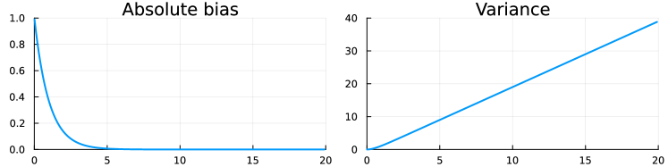
Figure 1: Absolute bias and variance of the Green–Kubo estimator (GK), in the simple setting of Subsection 2.3.

Half-Einstein estimators

A similar reasoning gives that the bias of the Half-Einstein estimator (HE) is given by

$$\mathbf{E}\left[\widehat{\rho}_{K,T}^{\rm HE}\right]-\rho=\frac{1}{T}\int_{0}^{T}(T-\theta)w\Bigl{(}\frac{\theta}{T}\Bigr{)}k(\theta)\,d\theta-1.$$

To obtain a practical formula for the variance, we first rewrite the estimator (HE) as follows:

$$\widehat{\rho}_{K,T}^{\rm HE}=\frac{1}{KT}\sum_{k=1}^{K}\int_{0}^{T}\int_{0}^{T-u}w\left\lparen\frac{u}{T}\right\rparen f(X^{k}_{s})g(X^{k}_{s+u})\,ds\,du.$$ (2.39)

Consider the particular setting of this subsection, with $f,g$ the identity functions and $K=1$. Taking the square in (2.39), taking the expectation, and using Isserlis’ theorem, we obtain the following expression for the variance:

$$\operatorname*{\mathbf{V}}\left[\widehat{\rho}_{K,T}^{\rm HE}\right]=\frac{1}{T^{2}}\int_{0}^{T}\!\!\int_{0}^{T}w\left(\frac{u}{T}\right)w\left(\frac{v}{T}\right)I(u,v)\,dv\,du-\mathbf{E}\left[\widehat{\rho}_{K,T}^{\rm HE}\right]^{2},$$

where

$$I(u,v):=\int_{0}^{T-u}\int_{0}^{T-v}\Bigl{(}k(u)k(v)+k(t+v-s-u)k(t-s)+k(t+v-s)k(t-s-u)\Bigr{)}\,dt\,ds.$$

The inner double integral $I(u,v)$ can be calculated explicitly by symbolic calculations, after which the outer double integral can be calculated by numerical quadrature. The absolute bias and the variance, for various weight functions encountered in the literature and for a range of values of $T$, are illustrated in Figure 2.

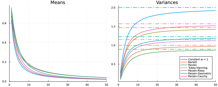
Figure 2: Absolute bias and variance of the Half-Einstein estimator (HE), in the simple setting of Subsection 2.3. The dashed lines correspond to the asymptotic values of the variances given by Proposition 2.7.

Weight function	Expression for $w(t)$ (for $0\leqslant t\leqslant 1$)
Constant	$w(t)=\mathbf{1}_{\{0\leqslant t\leqslant t\}}$
Bartlett	$w(t)=1-t$
Parzen	$w(t)=\begin{cases}1-6t^{2}+6t^{3},&t\leqslant 0.5\\ 2(1-t)^{3},&t>0.5\end{cases}$
Tukey–Hanning	$w(t)=\dfrac{1+\cos(\pi t)}{2}$
Parzen–Riesz	$w(t)=1-t^{2}$
Parzen–Geometric	$w(t)=\dfrac{1}{1+t}$
Parzen–Cauchy	$w(t)=\dfrac{1}{1+t^{2}}$

Table 3: Expression for various weight functions $w(t)$, defined as above on $0\leqslant t\leqslant 1$, and otherwise $0$; see [41] and references therein.

3 Control variates for fluctuation formulas

When used without modification, the estimators (GK) and (HE) presented from Section 2 can have a large variance. In this section, we construct and discuss some improved estimators based on control variates to calculate $\rho$ in (TC):

$$\rho=\langle f,-\mathcal{L}^{-1}g\rangle=\int_{0}^{+\infty}\mathbf{E}\bigl{[}f(X_{0})g(X_{t})\bigr{]}\,dt.$$ (3.1)

In particular, we consider three distinct ways of calculating (3.1) via a control variate approach. These are all based on replacing, in the estimators given in Section 2, the function $g$ or $f$ or both by other “smaller” functions involving approximate solutions to Poisson equations. By a slight abuse of terminology, we call control variates the functions used in place of $g$ or $f$ in the improved estimators. The three approaches studied in this section are summarized below:

• Forward control variate: based on replacing by a control variate the function $g$, which appears with a time dependence in the Green–Kubo formula (3.1) and in the related estimators (GK) and (HE). This approach is discussed in Subsection 3.1.

• Adjoint control variate: based on replacing by a control variate the function $f$, which acts only in the initial condition in the Green–Kubo formula (3.1) and in the related estimators (GK) and (HE). This approach is discussed in Subsection 3.2.

• Combined control variates: based on replacing both $f$ and $g$ by control variates, discussed in Subsection 3.3.

Throughout this section, we let $F^{*},G$ denote the solutions in $L^{2}_{0}(\mu)$ to

$$-\mathcal{L}^{*}F^{*}=f,$$ (3.2a)

$$-\mathcal{L}G=g.$$ (3.2b)

Since $(\mathrm{e}^{t\mathcal{L}})^{*}$ = $\mathrm{e}^{t\mathcal{L}^{*}}\in\mathcal{B}(L^{2}_{0}(\mu))$, decay estimates on the semigroup $\mathrm{e}^{t\mathcal{L}}$ such as Assumption 1 trivially extend to its adjoint. Thus, the well-posedness conditions discussed in Corollary 2.1 directly apply to (3.2a). We also denote by $\psi_{f}^{*}$ and $\psi_{g}$ approximations of the solutions to (3.2a) and (3.2b), respectively. These functions are assumed to belong to $L^{2}_{0}(\mu)$. Other integrability and regularity conditions are needed to make the variance of various estimators precise; see Corollaries 3.1 to 3.6. The concrete construction of these approximate solutions will be discussed in the next section. For convenience we also introduce

$$\zeta_{w}=\int_{0}^{1}(1-v)w(v)^{2}\,dv,$$ (3.3)

for the factor associated with a weight function $w$ that appears on the right-hand of the asymptotic variance formula (2.22). The three control variates studied in this section are summarized in Table 4.

$\Big{(}$ Control variate	Formula for $\rho=\langle f,-\mathcal{L}^{-1}g\rangle$
$\Big{(}$ Forward	$\displaystyle\rho={\color[rgb]{0.0,0.5,0.0}\langle f,\psi_{g}\rangle}+{\color[rgb]{1,0,1}\langle f,G-\psi_{g}\rangle}$
Estimators (3.6) or (3.7)	Variance GK (Corollary 3.1) $\propto\lVert f\rVert^{2}\mathcal{E}(G-\psi_{g}){\color[rgb]{1,0,0}T}$
(Subsection 3.1)	Variance HE (Corollary 3.2) $\propto\mathcal{E}(f)\mathcal{E}(G-\psi_{g})$
$\Big{(}$ Adjoint	$\displaystyle\rho={\color[rgb]{0.0,0.5,0.0}\langle\psi_{f}^{*},g\rangle}+{\color[rgb]{1,0,1}\langle f+\mathcal{L}^{*}\psi_{f}^{*},G\rangle}$
Estimators (3.10) or (3.12)	Variance GK (Corollary 3.3) $\propto\lVert f+\mathcal{L}^{*}\psi_{f}^{*}\rVert^{2}\mathcal{E}(G){\color[rgb]{1,0,0}T}$
(Subsection 3.2)	Variance HE (Corollary 3.4) $\propto\mathcal{E}(F^{*}-\psi_{f}^{*})\mathcal{E}(G)$
$\Big{(}$ Combined	$\displaystyle\rho={\color[rgb]{0.0,0.5,0.0}\langle\psi_{f}^{*},g\rangle+\langle f,\psi_{g}\rangle+\langle\psi_{f}^{*},\mathcal{L}\psi_{g}\rangle}+{\color[rgb]{1,0,1}\langle f+\mathcal{L}^{*}\psi_{f}^{*},G-\psi_{g}\rangle}$
Estimators (3.14) or (3.16)	Variance GK (Corollary 3.5) $\propto\lVert f+\mathcal{L}^{*}\psi_{f}^{*}\rVert^{2}\mathcal{E}(G-\psi_{g}){\color[rgb]{1,0,0}T}$
(Subsection 3.3)	Variance HE (Corollary 3.6) $\propto\mathcal{E}(F^{*}-\psi_{f}^{*})\mathcal{E}(G-\psi_{g})$

Table 4: Summary of the various control variates that we consider to approximate. In all the formulas, the functions $\psi_{f}^{*},\psi_{g}$ denote respectively approximations of the solutions $F^{*},G$ to the Poisson equations $-\mathcal{L}^{*}F^{*}=f$ and $-\mathcal{L}G=g$. The terms highlighted in dark green are the so-called “static” terms which can be evaluated via standard Monte Carlo methods, while the terms highlighted in magenta are the only ones containing the unknown functions $F^{*},G$. These are all of the form $\langle h,\mathcal{L}^{-1}\ell\rangle$, for appropriate functions $h,\ell$, and so they can be approximated using the estimators of Section 2.

3.1 Forward control variate

A simple calculation shows that

$$\rho=\langle f,-\mathcal{L}^{-1}g\rangle=\langle f,\psi_{g}\rangle+\langle f,G-\psi_{g}\rangle.$$ (3.4)

The first term on the right-hand side of (3.4), henceforth called the static term, corresponds to an approximation of $\rho$ obtained from the approximate solution $\psi_{g}$ to the Poisson equation, and can be computed by resorting to standard Monte Carlo algorithms sampling $\mu$. The second term is a correction term, which can be approximated using the estimators presented in Section 2. We next discuss estimators for this term and state some technical results which make precise the associated variances.

Static part

In low dimension, the average $\langle f,\psi_{g}\rangle$ can be estimated via deterministic methods or classical i.i.d. Monte Carlo sampling. When this is not possible, a Markov chain Monte Carlo (MCMC) approach can be employed:

$$\widehat{\rho}_{K,T}^{\rm static}(f,\psi_{g})=\frac{1}{KT}\sum_{k=1}^{K}\int_{0}^{T}f(X_{t}^{k})\psi_{g}(X_{t}^{k})\,dt.$$ (3.5)

In any case, the approximation of $\langle f,\psi_{g}\rangle$ is much simpler than expressions involving correlations, and various variance reduction methods can be used.

Green–Kubo

One possible estimator for the correction term in (3.4) is given by the usual Green–Kubo estimator (GK), which gives:

$$\widehat{\rho}_{K,T,\psi_{g}}^{\rm corr,GK}=\frac{1}{K}\sum_{k=1}^{K}\int_{0}^{T}f(X^{k}_{0})\Bigl{(}g(X^{k}_{t})+\mathcal{L}\psi_{g}(X_{t}^{k})\Bigr{)}\,dt.$$ (3.6)

We next state a result on the variance of the improved estimator (3.6), a straightforward result directly obtained from Proposition 2.3 by replacing $g$ with $g+\mathcal{L}\psi_{g}$.

Corollary 3.1 (Variance of improved GK estimator 1).

Assume that $f,g$ satisfy the conditions given in Proposition 2.3, and that $\psi_{g}\in L^{4}(\mu)$ with $\mathcal{L}\psi_{g}\in L^{2}_{0}(\mu)$ and $\chi_{\psi_{g}}\in L^{2}(\mu)$. Then,

$$\lim_{T\to\infty}T^{-1}\operatorname*{\mathbf{V}}\left\lparen\widehat{\rho}_{K,T,\psi_{g}}^{\rm corr,GK}\right\rparen=\frac{2}{K}\lVert f\rVert^{2}\Big{\langle}g+\mathcal{L}\psi_{g},-\mathcal{L}^{-1}(g+\mathcal{L}\psi_{g})\Big{\rangle}.$$

Recall from the discussion after Proposition 2.3 that bounds on the resolvent are typically of order $\lambda^{-1}$ where $\lambda$ is the smallest nonzero eigenvalue of the operator $\mathcal{L}$. Thus, the $g$ term in the expression for the asymptotic variance is of order $\lambda^{-1}\lVert g+\mathcal{L}\psi_{g}\rVert^{2}$. Corollary 3.1 thus suggests that the improved estimator is numerically useful when $\lVert g+\mathcal{L}\psi_{g}\rVert\ll\lVert g\rVert$, namely when the residual associated with the approximate solution of the Poisson equation is small enough.

Half Einstein

Another possible estimator for the correction term in (3.4) is the half Einstein estimator (HE):

$$\widehat{\rho}_{K,T,\psi_{g}}^{\rm corr,HE}=\frac{1}{TK}\sum_{k=1}^{K}\int_{0}^{T}\int_{0}^{t}w\left\lparen\frac{t-s}{T}\right\rparen f(X^{k}_{s})\Bigl{(}g(X^{k}_{t})+\mathcal{L}\psi_{g}(X_{t}^{k})\Bigr{)}\,ds\,dt.$$ (3.7)

The variance of (3.7) is made precise in the following corollary of Proposition 2.7.

Corollary 3.2 (Variance of improved HE estimator 1).

Assume that $f,g$ satisfy the conditions given in Proposition 2.7, and that $\psi_{g}\in L^{4}(\mu)$ with $\mathcal{L}\psi_{g}\in L^{4}(\mu)$ and $\chi_{\psi_{g}}\in L^{4}(\mu)$. Then,

$$\lim_{T\to+\infty}\operatorname*{\mathbf{V}}\left\lparen\widehat{\rho}_{K,T,\psi_{g}}^{\rm corr,HE}\right\rparen=\frac{4\zeta_{w}}{K}\langle f,-\mathcal{L}^{-1}f\rangle\langle g+\mathcal{L}\psi_{g},-\mathcal{L}^{-1}(g+\mathcal{L}\psi_{g})\rangle.$$

Computing either (3.6) or (3.7) requires evaluating the control variate $g+\mathcal{L}\psi_{g}$ at every step of the Monte Carlo simulation, which is an expensive computation. In the next section, we present a control variate approach with a lower computational cost, as it does not require evaluation at all steps.

3.2 Adjoint control variate

It is possible to devise a control variate which need not be evaluated at all steps of the Monte Carlo run. In particular, we construct a near-zero-cost control variate (i.e., zero-cost aside from the computation of the approximate solution to the Poisson equation), as it is only evaluated once at initial time. To this end, we first write (3.1) in terms of the adjoint:

$$\rho =\langle(-\mathcal{L}^{-1})^{*}f,g\rangle$$

$$=\langle\psi_{f}^{*},g\rangle+\langle F^{*}-\psi_{f}^{*},g\rangle$$ (3.8a)

$$=\langle\psi_{f}^{*},g\rangle+\langle f+\mathcal{L}^{*}\psi_{f}^{*},-\mathcal{L}^{-1}g\rangle.$$ (3.8b)

As in the previous section, the first term on the right-hand side is a static term that can be estimates with standard trajectory averages as,

$$\widehat{\rho}_{K,T}^{\rm static}(g,\psi_{f}^{*})=\frac{1}{KT}\sum_{k=1}^{K}\int_{0}^{T}g(X_{t}^{k})\psi_{f}^{*}(X_{t}^{k})\,dt,$$ (3.9)

while the second term can be approximated using the estimators presented in Section 2, as made precise below.

Green–Kubo

The second term in (3.8b) assumes the following estimator

$$\widehat{\rho}_{K,T,\psi_{f}}^{\rm corr,GK}=\frac{1}{K}\sum_{k=1}^{K}\int_{0}^{T}\left(f(X^{k}_{0})+\mathcal{L}^{*}\psi_{f}^{*}(X_{0}^{k})\right)g(X^{k}_{t})\,dt.$$ (3.10)

Note that this estimator requires the computation of the control variate $f+\mathcal{L}^{*}\psi_{f}^{*}$ only at the initial time, eliminating the need to evaluate the control variate at every step of the Monte Carlo simulation.

Corollary 3.3 (Variance of improved GK estimator 2).

Assume that $f,g$ satisfy the conditions given in Proposition 2.3, and that $\mathcal{L}^{*}\psi_{f}^{*}\in L^{4}(\mu)$. Then,

$$\lim_{T\to+\infty}T^{-1}\operatorname*{\mathbf{V}}\left\lparen\widehat{\rho}_{K,T,\psi_{f}}^{\rm corr,GK}\right\rparen=\frac{2}{K}\lVert f+\mathcal{L}^{*}\psi_{f}^{*}\rVert^{2}\big{\langle}g,-\mathcal{L}^{-1}g\big{\rangle}.$$ (3.11)

Note that $\mathcal{L}^{*}\psi_{f}^{*}$ automatically has average 0 with respect to $\mu$, since $\psi_{f}^{*}$ itself has average 0.

Half Einstein

The second term in (3.8b) assumes the following estimator

$$\widehat{\rho}_{K,T,\psi_{f}}^{\rm corr,HE}=\frac{1}{TK}\sum_{k=1}^{K}\int_{0}^{T}\int_{0}^{t}w\left(\frac{t-s}{T}\right)\Bigl{(}f\bigl{(}X^{k}_{s}\bigr{)}+\mathcal{L}^{*}\psi_{f}^{*}\bigl{(}X_{s}^{k}\bigr{)}\Bigr{)}g\bigl{(}X^{k}_{t}\bigr{)}\,ds\,dt.$$ (3.12)

Corollary 3.4 (Variance of improved HE estimator 2).

Assume that $f,g$ satisfy the conditions given in Proposition 2.7, and that $(\mathcal{L}^{-1})^{*}f\in L^{4}(\mu)$, $\psi_{f}^{*}\in L^{4}(\mu)$, $\mathcal{L}^{*}\psi_{f}^{*}\in L^{4}(\mu)$ and $\chi_{\psi_{f}^{*}}\in L^{4}(\mu)$. Then,

$$\lim_{T\to+\infty}\operatorname*{\mathbf{V}}\left\lparen\widehat{\rho}_{K,T,\psi_{f}}^{\rm corr,HE}\right\rparen=\frac{4\zeta_{w}}{K}\Big{\langle}f+\mathcal{L}^{*}\psi_{f}^{*},-\mathcal{L}^{-1}(f+\mathcal{L}^{*}\psi_{f}^{*})\Big{\rangle}\Big{\langle}g,-\mathcal{L}^{-1}g\Big{\rangle}.$$

3.3 Combining both control variates

By obtaining approximate solutions to both Poisson equations, we can apply both control variates simultaneously. By writing $-\mathcal{L}^{-1}g=\psi_{g}+(G-\psi_{g})$ in (3.8b), we obtain

$$\rho =\langle\psi_{f}^{*},g\rangle+\langle f+\mathcal{L}^{*}\psi_{f}^{*},G\rangle$$

$$=\langle\psi_{f}^{*},g\rangle+\langle f+\mathcal{L}^{*}\psi_{f}^{*},\psi_{g}\rangle+\langle f+\mathcal{L}^{*}\psi_{f}^{*},G-\psi_{g}\rangle$$

$$=\langle\psi_{f}^{*},g\rangle+\langle f,\psi_{g}\rangle+\langle\psi_{f}^{*},\mathcal{L}\psi_{g}\rangle+\langle f+\mathcal{L}^{*}\psi_{f}^{*},G-\psi_{g}\rangle.$$ (3.13)

The first three terms can be estimated directly using trajectory averages, while the last term can be approximated using the estimators in Section 2.

The GK improved estimator reads

$$\widehat{\rho}_{K,T,\psi_{f},\psi_{g}}^{\rm corr,GK}=\frac{1}{K}\sum_{k=1}^{K}\int_{0}^{T}\Bigl{(}f(X^{k}_{0})+\mathcal{L}^{*}\psi_{f}^{*}(X_{0}^{k})\Bigr{)}\Bigl{(}g(X^{k}_{t})+\mathcal{L}\psi_{g}(X_{t}^{k})\Bigr{)}\,dt.$$ (3.14)

Corollary 3.5 (Variance of improved GK estimator 3).

Assume that $f,g$ satisfy the conditions given in Proposition 2.3, and that in addition the conditions from Corollaries 3.1 and 3.3 hold. Then,

$$\lim_{T\to+\infty}T^{-1}\operatorname*{\mathbf{V}}\left\lparen\widehat{\rho}_{K,T,\psi_{f},\psi_{g}}^{\rm corr,GK}\right\rparen=\frac{2}{K}\lVert f+\mathcal{L}^{*}\psi_{f}^{*}\rVert^{2}\Big{\langle}g+\mathcal{L}\psi_{g},-\mathcal{L}^{-1}(g+\mathcal{L}\psi_{g})\Big{\rangle}.$$ (3.15)

The HE improved estimator reads

$$\widehat{\rho}_{K,T,\psi_{f},\psi_{g}}^{\rm corr,HE} =\frac{1}{TK}\sum_{k=1}^{K}\int_{0}^{T}\int_{0}^{t}w\left\lparen\frac{t-s}{T}\right\rparen\Bigl{(}f(X^{k}_{s})+\mathcal{L}^{*}\psi_{f}^{*}(X_{s}^{k})\Bigr{)}\Bigl{(}g(X^{k}_{t})+\mathcal{L}\psi_{g}(X_{t}^{k})\Bigr{)}\,ds\,dt.$$ (3.16)

Corollary 3.6 (Variance of improved HE estimator 3).

Assume that $f,g$ satisfy the conditions given in Proposition 2.7, and that in addition the conditions from Corollaries 3.2 and 3.4 hold. Then,

$$\lim_{T\to+\infty}\operatorname*{\mathbf{V}}\left\lparen\widehat{\rho}_{K,T,\psi_{f},\psi_{g}}^{\rm corr,HE}\right\rparen=\frac{4\zeta_{w}}{K}\Big{\langle}f+\mathcal{L}^{*}\psi_{f}^{*},-\mathcal{L}^{-1}(f+\mathcal{L}^{*}\psi_{f}^{*})\Big{\rangle}\Big{\langle}g+\mathcal{L}\psi_{g},-\mathcal{L}^{-1}(g+\mathcal{L}\psi_{g})\Big{\rangle}.$$

4 Applications

The aim of this section is to apply the control variate methods discussed in Section 3 to different systems in order to assess the effectiveness of the various estimators. We start by discussing in Subsection 4.1 the general approach for solving Poisson equations using neural networks. We then apply the method to the underdamped Langevin dynamics in Subsection 4.2, and to multiscale SDEs in Subsection 4.3.

4.1 Approximate solutions to Poisson equations with neural networks

We now discuss the overall strategy for approximating the solution to Poisson equations using PINNs. In particular, we discuss the loss function used and its discretization, and outline the common training strategy. More specific architectural choices, such as activation functions, featurization strategies and network topology are overviewed in the respective numerical application sections to come.

Loss function

Let us consider the following Poisson equation

$$-\mathcal{L}\phi(x)=f(x),\qquad x\in\mathcal{X},$$ (4.1)

with $\mathcal{X}\subset^{d}$, and $f\colon\mathcal{X}\to$. We denote by $\phi^{\mathrm{NN}}_{\theta}(x)$ the neural network approximation of $\phi$ parametrized by a set of parameters $\theta$. The pointwise loss function we consider is the mean squared error of the residual $r_{\theta}(x)=\mathcal{L}\phi^{\mathrm{NN}}_{\theta}(x)+f(x)$. At the continuous level, the loss function is then

$$\mathscr{L}(\theta)=\int_{\mathcal{X}}\left(\mathcal{L}\phi^{\mathrm{NN}}_{\theta}(x)+f(x)\right)^{2}\mu(dx).$$ (4.2)

In practice, the integral in (4.2) is approximated with a sum over the data points $\{\mathbf{x}^{n}\}_{n=1}^{N}\in^{d}$ at which the functions are evaluated, where the points are directly sampled from $\mu$ via rejection sampling. Additionally, we consider centered finite differences to approximate differential operators in $\mathcal{L}$ acting on $\phi$, as automatic differentiation becomes too cumbersome for derivatives of order 3 and higher. Thus, automatic differentiation is only used to take the gradient of the network with respect to the parameters during training. To this end, let $\mathcal{L}^{\Delta}$ denote the discretization of $\mathcal{L}$. Then, our loss function is of the form

$$\mathscr{L}(\theta)=\frac{1}{N}\sum_{n=1}^{N}\lvert\mathcal{L}^{\Delta}\phi^{\mathrm{NN}}_{\theta}(\mathbf{x}^{n})+f(\mathbf{x}^{n})\rvert^{2}.$$ (4.3)

Let us similarly define $\phi^{*}$ as the solution to the adjoint Poisson equation $-\mathcal{L}^{*}\phi^{*}=f^{*}$, with $\mathscr{L}^{*}(\theta)$ the associated loss function.

Training strategy

The same overall strategy was used to train the networks for both examples here presented. The training data consisted of $N$ points sampled from $\mu$ with rejection sampling. The computational cost associated with sampling the data points is negligible, allowing us to compute a stochastic approximation of the gradient with $N$ new points at every step. Since the usual overfitting risks associated with a finite training set therefore do not apply, we performed a fixed number of training steps and did not implement early stopping. We used Adam [17] as the optimizer.

The network topologies considered were simple networks with two dense hidden layers, and the same activation function throughout, in particular $\tanh$ for both examples. Other activation functions were explored, e.g. regularized ReLU-type functions such as gelu [gelu2023] were observed to perform marginally better than $\tanh$, however at an increased computational cost. The addition of the second hidden layer significantly improves the quality of training, while still retaining a sufficiently low cost. Based on numerical observations from experimental runs, width has a more significant impact on the quality of training than depth for a fixed number of network parameters.

All training parameters are made precise in Table 5 for the Langevin dynamics example, and Table 8 for the multiscale example.

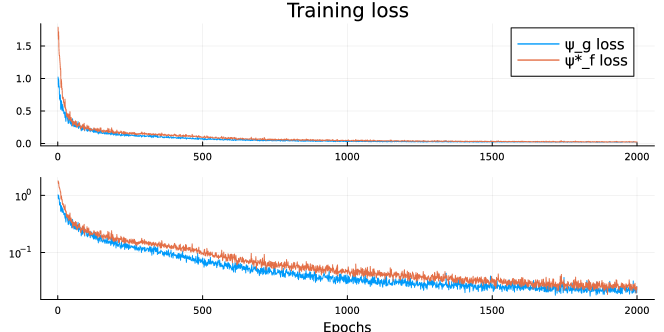
Figure 3: Training loss over epochs for the 2D Langevin dynamics for both $\psi_{g}$ and $\psi_{f}^{*}$ approximate solutions. Top: linear scale. Bottom: logarithmic y-axis.

The same training routine was used to approximate $\phi$ and $\phi^{*}$. Figure 3 shows the training loss as a function of training steps for both approximations for the Langevin dynamics example.

4.2 Application to the underdamped Langevin dynamics

We apply in this section the methodology to compute the mobility of the two-dimensional underdamped Langevin dynamics. We start by giving a brief description of the system in Subsection 4.2.1, followed by a presentation of the numerical results in Subsection 4.2.2.

4.2.1 Description of the system

Let us briefly describe the system in consideration. The two-dimensional Langevin dynamics evolves the positions $q=(q_{1},q_{2})\in\mathbb{T}^{2}$ and momenta $p=(p_{1},p_{2})\in^{2}$ according to the following SDE:

$$\begin{split}\begin{cases}dq_{t}=M^{-1}p_{t}\,dt,\\ dp_{t}=-\nabla V(q_{t})\,dt-\gamma M^{-1}p_{t}\,dt+\sqrt{\dfrac{2\gamma}{\beta}}\,dW_{t}.\end{cases}\end{split}$$ (4.4)

where $M\in^{2\times 2}$ denotes the mass matrix, $\gamma>0$ the friction coefficient, $\beta>0$ the inverse temperature and $V$ a smooth periodic potential energy function. The dynamics (4.4) admits the following infinitesimal generator

$$\mathcal{L}=p^{\mathsf{T}}M^{-1}\nabla_{q}-\nabla V^{\mathsf{T}}\nabla_{p}+\gamma(-p^{\mathsf{T}}M^{-1}\nabla_{p}+\beta^{-1}\Delta_{p}),$$ (4.5)

and is ergodic with respect to the Boltzmann–Gibbs measure $\mu$:

$$\mu(dq\,dp)=\frac{1}{Z}\mathrm{e}^{-\beta H(q,p)}\,dq\,dp,\qquad Z=\int_{\mathcal{X}}\mathrm{e}^{-\beta H(q,p)}dq\,dp.$$ (4.6)

The mobility in the direction $\mathbf{e}$ is defined as the proportionality constant between the magnitude $\eta$ of an exerted constant force proportional to $\mathbf{e}$, and the induced drift velocity $\mathbf{E}(f_{\mathbf{e}})$ in this direction, with $f_{\mathbf{e}}=\mathbf{e}^{\mathsf{T}}M^{-1}p$. The relationship is linear for $\eta\to 0$, as dictated by linear response theory; see for instance [10, Chapter 8] and [MR3509213, Section 5]. Through an equilibrium formulation of the linear response based on velocity autocorrelations [35], it can in particular be written in terms of the solution to a Poisson equation:

$$\rho=\langle\phi,\beta f_{\mathbf{e}}\rangle,$$ (4.7)

and

$$-\mathcal{L}\phi(q,p) =f_{\mathbf{e}}(q,p).$$ (4.8)

It can similarly be defined in terms of the $L^{2}(\mu)$-adjoint as $\rho=\langle\phi^{*},f_{\mathbf{e}}\rangle$, where $-\mathcal{L}^{*}\phi^{*}=\beta f_{\mathbf{e}}$. Note that the mobility is proportional up to factor $\beta$ to the self-diffusion coefficient through Einstein’s relation; see [36]. The points $\{\mathbf{x}^{n}\}_{n=1}^{N}=(q_{1},q_{2},p_{1},p_{2})_{n}\in^{4}$ are i.i.d. according to the target measure $\mu$, sampled in practice using rejection sampling.

4.2.2 Numerical results

We consider the following nonseperable potential energy function

$$V(q_{1},q_{2})=-\frac{\cos(2q_{1})+\cos(q_{2})}{2}-\delta\cos(q_{1})\cos(q_{2}),$$ (4.9)

with $\delta\in$ the degree of nonseparability. The numerical results here presented correspond to the value $\delta=0.5$. Additionally, we set the physical parameters $\beta=\gamma=1$ and $M=\operatorname{Id}$.

Structure of the network

Aside from the general training strategy outlined in Subsection 4.1, the architecture for this example also includes a featurization layer. We employ a transformation on the inputs in the form of a “functional layer”: the input $(q_{1},q_{2},p_{1},p_{2})$ is transformed into a 7-node input by the functions:

$$\mathrm{featurization}\left\lparen q_{1},q_{2},p_{1},p_{2}\right\rparen=\left\lparen\sin(q_{1}),\cos(q_{1}),\sin(q_{2}),\cos(q_{2}),p_{1},p_{2},\frac{p_{1}^{2}+p_{2}^{2}}{2}\right\rparen$$ (4.10)

which is then fed to the first trainable layer; see Figure 4 for an illustration of the network topology. The periodic nature of the positions is encoded by the sines and cosines in the featurization layer, while the momenta are included directly. Lastly, the kinetic energy term was observed to be a meaningful feature in improving training, and is thus considered.

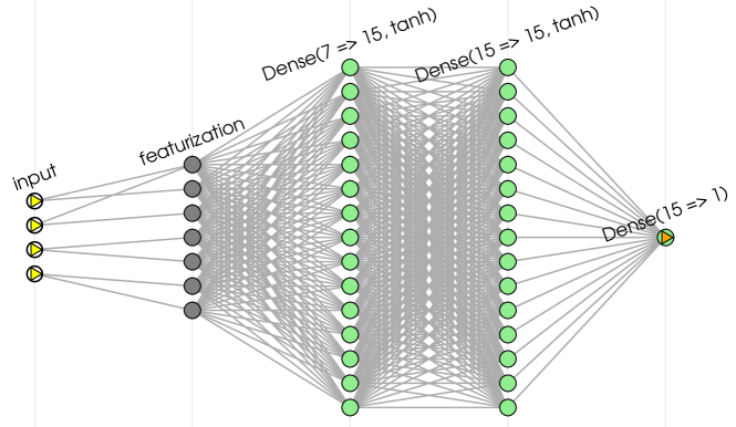
Figure 4: Neural network architecture for the two-dimensional Langevin dynamics. The input undergoes a transformation through a feature extraction function, which is then fed to the two hidden layers, both of which are dense and employ $\tanh$ as the activation function.

Monte–Carlo simulations

For each estimator, we used the BAOAB splitting scheme [20], with an integration time of $T=5$ for Green–Kubo and $T=10$ for Half Einstein, with timestep $\Delta t=0.01$ for both. We ran $K=1000$ independent realizations of the dynamics in order to empirically estimate the variance. Initial conditions for each realization were also sampled from $\mu$ using rejection sampling.

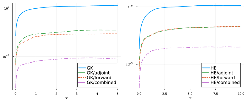
Figure 5: Asymptotic variance over time for all estimators for the two-dimensional Langevin dynamics. Left: Green–Kubo estimators. Right: Half Einstein estimators. For Green–Kubo, the asymptotic variance is defined as the variance divided by time, while the two coincide for Half Einstein.

Parameter	Value
Adam learning rate	0.002
Batch size	500
Number of iterations	2,000

Table 5: Training parameters for training the network for the two-dimensional Langevin dynamics.

Simulation results are illustrated in Figure 5, which shows the variance as a function of time for all 8 estimators considered. A plot of the asymptotic variance is also shown, which corresponds to the variance divided by time for Green–Kubo estimators, while it coincides with the variance for Half Einstein estimators. A summary of the results at time $T=10$ is compiled in Table 6, which provides a quantitative metric for assessing the viability of each estimator. In particular, it shows the computational runtime, the variance and the cost (defined as the product of runtime and variance) for each estimator.

The numerical results suggest that the use of both control variates (for both GK and HE) is the best option according to the cost. This, however, requires a decently trained network, as the forward adjoint is computed every step of the Monte Carlo simulation, thus it must provide enough variance reduction in order to offset the additional computational cost. The Green–Kubo adjoint estimator, on the other hand, is a (near) “zero-cost” control variate, as it is only evaluated once. This suggests that it is much more forgiving of nonoptimal training runs.

Estimator	Runtime	Variance at $T=5$	Cost
GK (GK)	$1$	$1$	$1$
GK/adjoint (3.10)	$0.957$	$0.0294$	$0.0281$
GK/forward (3.6)	$22.9$	$0.0172$	$0.394$
GK/both (3.14)	$25.1$	$0.000465$	$0.0117$

Table 6: Computational runtimes required to compute the self-diffusion coefficient for the two-dimensional Langevin dynamics and associated variances at time $T=5$, based on $K=1000$ realizations of the dynamics. The cost is defined as the runtime times the variance. Values are normalized in terms of the standard Green–Kubo estimator runtime of $0.156734$ seconds, and associated variance $7.330798$.

Estimator	Runtime	Variance at $T=10$	Cost
HE (HE)	$1$	$1$	$1$
HE/adjoint (3.12)	$23.9$	$0.0140$	$0.336$
HE/forward (3.7)	$22.6$	$0.0147$	$0.332$
HE/both (3.16)	$44.6$	$0.000246$	$0.0109$

Table 7: Computational runtimes required to compute the self-diffusion coefficient for the two-dimensional Langevin dynamics and associated variances at time $T=10$, based on $K=1000$ realizations of the dynamics. The cost is defined as the runtime times the variance. Values are normalized in terms of the standard Half Einstein estimator runtime of $0.296764$ seconds, and associated variance $1.312950$.

4.3 Application to multiscale differential equations

The aim of this subsection is to present an application of the control variate approaches studied in Section 3, with slight adjustments, to multiscale stochastic differential equations. We first describe briefly, in Subsection 4.3.1, the method of homogenization for multiscale SDEs. Then, in Subsection 4.3.2, we explain how the control variate approaches from Section 3 can be applied for the calculation of the effective coefficients of the homogenized equation. Finally, in Subsection 4.3.3, we illustrate the performance of the method on a concrete example.

4.3.1 Homogenization for multiscale SDEs

In this section, we give a concise description of the method of homogenization for multiscale SDEs in a simplified setting. We refer to [MR2382139, Chapter 11] for a more complete overview of the subject, and to [MR2382139, Chapter 18] and [MR1872736, MR1988467] for rigorous analyses. Consider the following multiscale system with state space ${}^{d_{x}}\times^{d_{y}}$, for some small parameter $\varepsilon>0$:

$$\left\{\begin{aligned} dX&=\frac{1}{\varepsilon}f(X,Y)\,dt,\\ dY&=\frac{1}{\varepsilon^{2}}g(X,Y)\,dt+\frac{1}{\varepsilon}\alpha(X,Y)\,dW_{t},\end{aligned}\right.$$ (4.11)

Here we assume that $f\colon^{d_{x}}\times^{d_{y}}\to^{d_{x}}$, $g\colon^{d_{x}}\times^{d_{y}}\to^{d_{y}\times d_{w}}$ and $\alpha\colon^{d_{x}}\times^{d_{y}}\to^{d_{y}\times d_{w}}$ are smooth functions, and that $(W_{t})$ is a standard Brownian motion in ${}^{d_{w}}$. Denote by $\varepsilon^{-2}\mathcal{L}^{x}$ the generator associated with the fast process $Y$ when $X$ is frozen:

$$\mathcal{L}^{x}=g(x,y)\cdot\nabla_{y}+\frac{1}{2}\alpha(x,y)\alpha(x,y)^{\mathsf{T}}:\nabla_{y}\nabla_{y}.$$

The theory of homogenization for multiscale SDEs states that, under appropriate conditions, the slow process $(X_{t})_{t\geqslant 0}$ is well approximated by the solution $(\overline{X}_{t})_{t\geqslant 0}$ to a simplified, single-scale stochastic differential equation. This is the content of the following result where, for a vector-valued function $f$, the notation $\nabla f$ refers to the matrix with entry $(i,j)$ equal to $\partial_{j}f_{i}$. We refer to [33, Chapter 18] for a rigorous proof in a simplified periodic setting, and the references discussed in [33, Chapter 18.4] for more general results.

Theorem 4.1 (Homogenization for SDEs).

Suppose that, for all $x\in^{d_{x}}$, there is a unique ergodic distribution $\mu^{x}(dy)$ of the fast process when $x$ is frozen, and additionally that

$$\forall x\in^{d_{x}},\qquad\int_{{}^{d_{x}}}f(x,y)\,\mu^{x}(dy)=0.$$

Then, in the limit $\varepsilon\to 0$, the slow process $(X_{t})_{t\geqslant 0}$ converges weakly in $C([0,T])$ to the solution of

$$d\overline{X}=F(\overline{X})+A(\overline{X})\,dV_{t},$$ (4.12)

where $V_{t}$ is a standard Browian motion and

$$F(x)=\int_{{}^{d_{y}}}\nabla_{x}\Phi(x,y)\,f(x,y)\,\mu^{x}(dy)\in^{d_{x}},\qquad A(x)A(x)^{\mathsf{T}}=A^{0}(x)+A^{0}(x)^{\mathsf{T}}\in^{d_{x}\times d_{x}},$$

with

$$A^{0}(x)=\int_{{}^{d_{y}}}f(x,y)\otimes\Phi(x,y)\,\mu^{x}(dy).$$

Here $\Phi$ is a solution to $-\mathcal{L}^{x}\Phi(x,y)=f(x,y).$

In many applications of multiscale SDEs, the coefficients $g$ and $a$ of the fast process in (4.11) are independent of $X$. This simplified setting, or a variation thereof where the drift and diffusion coefficients of the fast process also include lower order terms allowed to depend on $X$, is often considered in the literature, for example in numerical works [MR1980483, weinan2005analysis]. In this section, we assume for simplicity that $g=g(y)$ and $a=a(y)$. In this case, the generator of the fast process in (4.11) is independent of $x$, and so is the associated invariant measure for the fast process. Therefore, we drop the superscript $x$ from the notation $\mathcal{L}^{x}$ and $\mu^{x}$. Since formally $\nabla_{x}\mathcal{L}^{-1}=\mathcal{L}^{-1}\nabla_{x}$, the coefficients of the homogenized equation (4.12) are of the form (TC). More precisely, the components of the coefficients $F$ and $A^{0}$ can be written as

$$F_{i}(x)=\sum_{j=1}^{d_{x}}\Bigl{\langle}f_{j}(x,\,\cdot\,),-\mathcal{L}^{-1}\mathfrak{h}_{ij}(x,\,\cdot\,)\Bigr{\rangle},\qquad A^{0}_{ij}(x)=\Bigl{\langle}f_{i}(x,\,\cdot\,),-\mathcal{L}^{-1}f_{j}(x,\,\cdot\,)\Bigr{\rangle},\qquad$$ (4.13)

where $\mathfrak{h}_{ij}(x,\,\cdot\,)=\partial_{x_{j}}f_{i}(x,\,\cdot\,)$, and with $\langle\,\cdot\,,\,\cdot\,\rangle$ the inner product with respect to $L^{2}(\mu)$, with $x$ viewed as a fixed parameter. It follows from (4.13) that the homogenized coefficients can be approximated using estimators based on the Green–Kubo formula (1.4), such as those studied in Section 2. Indeed, this constitutes the basic idea behind the so-called heterogeneous multiscale method for multiscale SDEs [MR1980483, weinan2005analysis], a numerical method for solving (4.11) based on the resolution of the homogenized dynamics (4.12) using a classical integration scheme for SDEs, combined with the calculation, at each time step, of the effective coefficients $F,A^{0}$ using an estimator similar to the one studied in Subsection 2.2. The variance reduction method we describe in Subsection 4.3.2 is based on the specific estimators given in Section 3, but we note that it can easily be adapted to the estimators used within the heterogeneous multiscale method, such as those given in [weinan2005analysis, Section 3.1].

4.3.2 Control variate approaches for calculating the effective coefficients

In this section, we describe how the control variate approaches described in Section 3 can be employed for the calculation of the coefficients of the homogenized equation (4.12). The main difference with the other examples considered so far is the presence of an $x$-dependence in (4.13) and the associated Poisson equations

$$-\mathcal{L}\mathscr{H}_{ij}(x,y)=\mathfrak{h}_{ij}(x,y),\qquad-\mathcal{L}\mathscr{F}_{i}(x,y)=f_{i}(x,y),$$ (4.14)

as well as in the associated adjoint equation

$$-\mathcal{L}^{*}\mathscr{F}^{*}_{i}(x,y)=f_{i}(x,y).$$ (4.15)

The control variate methods described in Section 3 require approximate solutions to (4.14) or (4.15) or both. We next describe two possible approaches for constructing these approximate solutions:

• A first approach would be to solve the Poisson equations – (4.14) or (4.15) or both, depending on which method from Section 3 is considered – for each fixed $x$ separately as needed. Combined with a classical time-stepping algorithm for the homogenized equation (4.12), this would lead to a numerical method where a number of Poisson PDEs in dimension $d_{y}$ must be solved at each time step, much like the method studied in [MR3683698].

• An alternative approach, used in Subsection 4.3.3, is to solve the Poisson equations (4.14) for all $x\in^{d_{x}}$ and all vector components simultaneously. This is not simple to achieve using traditional PDE solvers, but simple to implement using neural networks. For example, in order to numerically solve the second equation in (4.14), we search for an approximate vector-valued solution $\mathscr{F}^{\rm NN}(x,y;\theta)$ within a class of functions parametrized by a neural network with parameters $\theta$. The vector of parameters $\theta$ is found by minimizing the following loss function

  $$\mathscr{L}(\theta)=\int_{{}^{d_{x}}\times^{d_{y}}}\sum_{i=1}^{d_{x}}\Bigl{\lvert}f_{i}(x,y)+\mathcal{L}\mathscr{F}^{\rm NN}_{i}(x,y;\theta)\Bigr{\rvert}^{2}\,\nu(dx)\,\mu(dy),$$ (4.16)

  where $\mu$ is, as before, the invariant probability measure associated with the fast processes in (4.11), and $\nu\in\mathcal{P}(^{d_{x}})$ is a probability measure on ${}^{d_{x}}$ that must be fixed a priori as part of the method. A natural choice, when ${}^{d_{x}}$ is a compact state space, is to let $\nu$ be the uniform distribution on ${}^{d_{x}}$. When ${}^{d_{x}}$ is non-compact, the choice of $\nu$ determines the region of ${}^{d_{x}}$ where we wish $\mathscr{F}^{\rm NN}(x,\,\cdot\,;\mathbf{c})$ to be a good approximation of the exact solution $\mathscr{F}(x,\,\cdot\,)$, and where variance reduction can be expected as a result. In practice, the loss function (4.16) of course needs to be discretized, for example by estimating the integral via Monte Carlo sampling.

To conclude this subsection, let us mention that it is not necessary to solve the first equation in (4.14) explicitly. Indeed, the function $\mathscr{H}_{ij}(x,y)$ is the $x$-gradient of $\mathscr{F}_{i}(x,y)$, and so a numerical approximation of $\mathscr{H}_{ij}(x,y)$ can be obtained by taking the $x$-gradient of $\mathscr{F}^{\rm NN}_{i}(x,y;\theta)$.

4.3.3 Numerical example

In this section, we illustrate the performance of the control variate strategies presented in Section 3, when the approximate solutions to Poisson equations are calculated simultaneously for all $x$ by a neural network approach. We consider the following simple example of a multiscale SDE, taken from [MR2382139, Section 11.7.7], to which we refer for additional context:

$$\left\{\begin{aligned} dX_{1}&=\frac{1}{\varepsilon}Y_{1}\,dt\,,\\ dX_{2}&=\frac{1}{\varepsilon}Y_{2}\,dt\,,\\ dX_{3}&=\frac{1}{\varepsilon}(X_{1}Y_{2}-X_{2}Y_{1})\,dt\,,\\ dY_{1}&=-\frac{Y_{1}}{\varepsilon^{2}}\,dt-\alpha\frac{Y_{2}}{\varepsilon^{2}}\,dt+\frac{1}{\varepsilon}dW^{1}_{t}\,,\\ dY_{2}&=-\frac{Y_{2}}{\varepsilon^{2}}\,dt+\alpha\frac{Y_{1}}{\varepsilon^{2}}\,dt+\frac{1}{\varepsilon}dW^{2}_{t}\,,\end{aligned}\right.$$ (4.17)

where $\alpha>0$ and $W^{1},W^{2}$ are standard independent Brownian motions. In this example, $d_{x}=3$ and $d_{y}=2$, so that the total dimension is equal to 5. An application of Theorem 4.1 leads to the following homogenized equation [MR2382139, Section 11.7.7]:

$$\left\{\begin{aligned} d\overline{X}_{1}&=\frac{1}{1+\alpha^{2}}\bigl{(}dV^{1}_{t}-\alpha\,dV^{2}_{t}\bigr{)}\,,\\ d\overline{X}_{2}&=\frac{1}{1+\alpha^{2}}\bigl{(}dV^{2}_{t}+\alpha\,dV^{1}_{t}\bigr{)}\,,\\ d\overline{X}_{3}&=\frac{1}{1+\alpha^{2}}\,dt+\frac{1}{1+\alpha^{2}}\Bigl{(}\bigl{(}\alpha\overline{X}_{1}-\overline{X}_{2}\bigr{)}\,dV^{1}_{t}+\bigl{(}\alpha\overline{X}_{2}+\overline{X}_{1}\bigr{)}\,dV^{2}_{t}\Bigr{)}.\end{aligned}\right.$$ (4.18)

In this numerical experiment, we fix $\alpha=1$ and compare the performance of the estimators given in Sections 2 and 3 for the computation of the homogenized coefficients. To this end, we solve the Poisson equations (both the forward equations involving $\mathcal{L}$, and the adjoint equations involving $\mathcal{L}^{*}$), simultaneously for all $x$. Furthermore, we solve the vector-valued Poisson equations simultaneously for all the components. For example, in order to solve the Poisson equations

$$-\mathcal{L}\mathscr{F}(x,\,\cdot\,)=f(x,\,\cdot\,),$$ (4.19)

with $f(x,y)\in^{3}$ the drift of the slow process, we use the neural network architecture illustrated in Figure 6. The neural network comprises 5 inputs, corresponding to the five variables $(x_{1},x_{2},x_{3},y_{1},y_{2})$, and three outputs, corresponding to the three components of the vector valued solution. For the measure $\nu$, we take the uniform distribution over the cube $[-4,4]^{3}$, and for $\mu$ we take the invariant measure of the fast processes. Since $(Y_{1},Y_{2})$ is an Ornstein–Uhlenbeck process, it follows from [MR2313847, Chapter 9] that the latter probability measure is given by the normal distribution $\mathcal{N}\left(0,\frac{1}{2}\operatorname{I}_{2}\right)$. The other training parameters are given in Table 8.

Having calculated approximate solutions to (4.19) and its adjoint counterpart, we then fix a value for $(X_{1},X_{2},X_{3})=(-0.0057,1.73,-1.04)$, randomly drawn from the standard normal distribution in dimension 3, and evaluate the quality of variance reduction for the estimators in Section 3, when these are used to calculate the homogenized coefficients for this particular value of $(X_{1},X_{2},X_{3})$. The static parts of all the estimators in Section 3 are calculated by numerical quadrature.

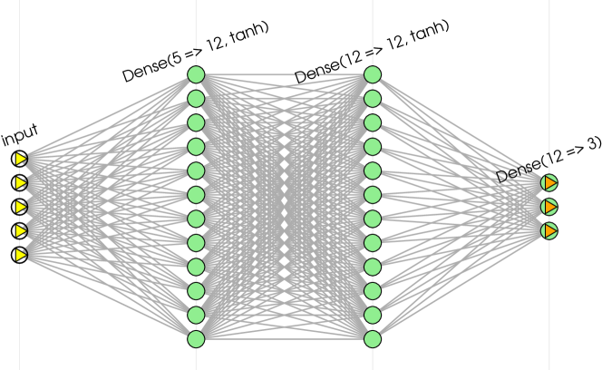
Figure 6: Neural network architecture employed for solving the (vector-valued) Poisson equation (4.19). Only $\tanh$ activation functions were used for this example.

Parameter	Value
Adam learning rate	0.002
Batch size	1,000
Number of iterations	1,000

Table 8: Training parameters for minimizing the loss function (4.16) in Subsection 4.3.3. At each of the 1,000 iterations, 1,000 samples are drawn independently from the probability measure $\mu\otimes\nu$. A step of ADAM is then performed based on the gradient of the loss function (4.16) calculated with the learning rate $0.002$.

The time required on a personal laptop to evaluate all the estimators from Section 3, not including the time required to train the neural networks, is presented in Tables 9 and 10 for $K=1000$ realizations. To produce these numerical results, an Euler–Maruyama discretization with a time step equal to $0.01\varepsilon^{2}$ was employed to integrate the fast dynamics, with the slow variables frozen at the value given above. It appears from the tables that the estimators using adjoint control variates are faster to evaluate than those using forward control variates, and this difference is especially pronounced for the Green–Kubo estimators. This is expected, as the estimator (3.10) requires to evaluate the control variate only at the initial time.

The tables also present the variance of all the estimators with $K=1$ realization, when the integration time for the fast dynamics is set to $T/\varepsilon^{2}=5$. These variances were calculated empirically based on 1,000 independent realizations. The third column, which contains the product of the runtime with the variance, is a measure of the cost, as in Subsection 4.2. From this column we observe that, both for the Green–Kubo and for the half-Einstein estimators, the combined control variate method from Subsection 3.3 performs best. Furthermore the variance reduction obtained with the forward and adjoint control variates are similar.

Estimator	Runtime [s]	Variance at $T/\varepsilon^{2}=5$	Runtime $\times$ Variance
GK (GK)	0.179	29.382	5.27
GK/forward (3.6)	13.785	0.206	2.85
GK/adjoint (3.10)	0.248	0.376	0.0935
GK/combined (3.14)	16.276	0.00306	0.0497

Table 9: Computational time required to calculate the homogenized drift and diffusion coefficients associated with the multiscale system (4.17), based on $K=1000$ realizations of the fast dynamics over a time horizon $T/\varepsilon^{2}=5$ and for one fixed value of $(X_{1},X_{2},X_{3})=(-0.0057,1.73,-1.04)$.

Estimator	Runtime [s]	Variance at $T/\varepsilon^{2}=5$	Runtime $\times$ Variance
HE (HE)	0.959	3.44555	3.31
HE/forward (3.7)	15.465	0.03678	0.569
HE/adjoint (3.12)	4.03	0.04346	0.175
HE/combined (3.16)	17.697	0.00066	0.0117

Table 10: Computational time required to calculate the homogenized drift and diffusion coefficients associated with the multiscale system (4.17), based on $K=1000$ realizations of the fast dynamics over a time horizon $T/\varepsilon^{2}=5$.

The variances associated with all the estimators, as a function of time, are illustrated in Figures 7 and 8 for the Green–Kubo and Half–Einstein estimators, respectively. These figures confirm the trends already observed in Tables 9 and 10. In particular, whether for Green–Kubo or half-Einstein estimators, combining both control variates as in (3.14) and (3.16) yields the largest variance reduction. The figures also illustrate that the variance reduction obtained with the forward or adjoint control variates are similar.

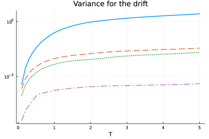
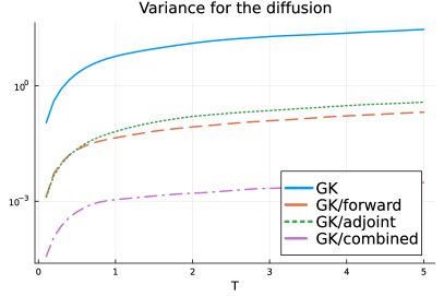
Figure 7: Variances of the Green–Kubo estimators presented in Section 3, when these are used to calculate the coefficients of the homogenized equation associated to (4.11). These values were calculated based on $K=1000$ realizations of each estimator.

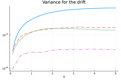
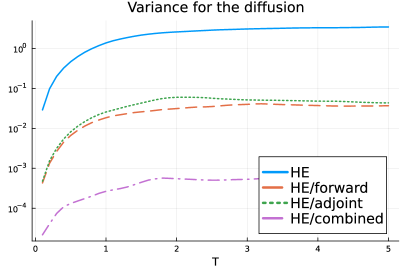
Figure 8: Variances of the half-Einstein estimators presented in Section 3, when these are used to calculate the coefficients of the homogenized equation associated to (4.11). These values were calculated based on $K=1000$ realizations of each estimator.

5 Extensions and perspectives

Let us conclude this work by discussing possible extensions and future directions for the results here presented. We have successfully shown that neural networks (in particular PINNs) can be an effective tool for constructing control variates via approximating Poisson equations, for problems well-posed enough. The main point of our approach was to construct simple, easy-to-train and inexpensive-to-evaluate networks to be used as control variates, evaluated alongside Monte Carlo simulations. The key point is that the network must be simple enough so that it is reasonably inexpensive to train and evaluate, while still providing significant variance reduction in order justify the additional computational cost. In other words, the cost (i.e. product of runtime and variance) must be less than that of the standard estimator.

There are several directions for extending the work. While possible, high-order nested automatic differentiation remains a nontrivial challenge, and is generally not an off-the-shelf tool, particularly for high-dimensional systems requiring batched training. Another possible direction is to further optimize the network’s cost-to-variance reduction ratio, in particular by further exploring featurization approaches, which can potentially increase the network’s efficiency without significantly increasing cost. Lastly, another possible extension of this method is for computing the mobility in the underdamped limit $\gamma\to 0$, particularly in the case of nonseparable potentials, which has been a challenge in the literature [32].

Appendix A Extension to general weights

We state here some technical results which generalize the results of Proposition 2.7. We first state an assumption which will be used in the results to come.

Assumption 2 (Decay estimates of the semigroup in $L^{4}(\mu)$).

There exist positive constants $L_{4}$ and $\lambda_{4}$ such that, for all $\varphi\in L^{4}_{0}(\mu)$ and all $t\geqslant 0$,

$$\left\lVert\mathrm{e}^{t\mathcal{L}}\varphi\right\rVert_{L^{4}_{0}(\mu)}\leqslant L\mathrm{e}^{-\lambda t}\left\lVert\varphi\right\rVert_{L^{4}_{0}(\mu)}.$$ (A.1)

Assumption 2 extends the semigroup decay estimates of Assumption 1 from $L^{2}(\mu)$ to $L^{4}(\mu)$, a necessary estimate in Lemma A.1 below. By [19, Theorem 2.2], see also [9, Theorem 1.3] and the discussion in [pavliotis2011applied, Section 2.6], the exponential convergence estimate in $L^{2}_{0}(\mu)$ given in Assumption 1 implies similar exponential convergence estimates in $L^{p}_{0}(\mu)$, for all $p\in[1,\infty)$ by an interpolation argument. The same assumption is made on $\mathcal{L}^{*}$, and can be shown to hold using the same interpolation argument as above.

Lemma A.1 (Continuity estimate).

Suppose that Assumption 2 holds true, and assume that $w$ is continuous at $0$. Assume additionally that $f,g\in L^{4}_{0}(\mu)$. Then, it holds that

$$\limsup_{T\to+\infty}\mathbf{E}\left[\left\lvert\widehat{\rho}_{K,T}^{\rm HE}\right\rvert^{2}\right]\leqslant\frac{L^{2}\lVert f\rVert^{2}_{L^{4}(\mu)}\lVert g\rVert^{2}_{L^{4}(\mu)}}{K}\left\lparen\frac{\lvert w(0)\rvert^{2}}{\lambda^{2}}+\frac{2}{\lambda}\int_{0}^{1}w(u)^{2}(1-u)\,du\right\rparen.$$ (A.2)

Remark A.2.

In contrast with the result of Proposition 2.7, in Lemma A.1 we make no regularity assumption on the derivatives of the weight function $w$.

Proof.

As in the proof of Proposition 2.7, we consider $K=1$ and use the simplified notation $\widehat{\rho}_{T}$ for the estimator.

If the right-hand side of (A.2) is infinite, then the inequality is satisfied, so we assume from now on that this term is finite. We first rewrite, for $\widehat{\rho}_{T}$ defined in (2.23),

$$\mathbf{E}\left[\left\lvert\widehat{\rho}_{T}\right\rvert^{2}\right]=T^{2}\int_{0}^{1}\!\!\int_{0}^{1}\!\!\int_{0}^{\tau}\!\!\int_{0}^{t}w(t-s)w(\tau-\varsigma)\mathbf{E}\Bigl{[}f(X_{sT})f(X_{\varsigma T})g(X_{tT})g(X_{\tau T})\Bigr{]}\,ds\,d\varsigma\,dt\,d\tau.$$ (A.3)

Fix $0\leqslant a\leqslant b\leqslant c\leqslant d\leqslant T$, as well as bounded functions $h_{1},h_{2},h_{3},h_{4}\in L^{4}_{0}(\mu)$. Conditioning successively on information at times $c$, $b$ and then $a$, we obtain that

$$\mathbf{E}\bigl{[}h_{1}(X_{a})h_{2}(X_{b})h_{3}(X_{c})h_{4}(X_{d})\bigr{]} =\mathbf{E}\left[h_{1}(X_{a})h_{2}(X_{b})\left(h_{3}\mathrm{e}^{(d-c)\mathcal{L}}h_{4}\right)(X_{c})\right]$$

$$=\mathbf{E}\left[h_{1}(X_{a})\left(h_{2}\mathrm{e}^{(c-b)\mathcal{L}}\left(h_{3}\mathrm{e}^{(d-c)\mathcal{L}}h_{4}\right)\right)(X_{b})\right]$$

$$=\mathbf{E}\left[h_{1}(X_{a})\mathrm{e}^{(b-a)\mathcal{L}}\left(h_{2}\mathrm{e}^{(c-b)\mathcal{L}}\left(h_{3}\mathrm{e}^{(d-c)\mathcal{L}}h_{4}\right)\right)(X_{a})\right]$$

$$=\left\langle h_{1},\mathrm{e}^{(b-a)\mathcal{L}}\left(h_{2}\mathrm{e}^{(c-b)\mathcal{L}}\left(h_{3}\mathrm{e}^{(d-c)\mathcal{L}}h_{4}\right)\right)\right\rangle$$

$$=\left\langle h_{2}\mathrm{e}^{(b-a)\mathcal{L}^{*}}h_{1},\mathrm{e}^{(c-b)\mathcal{L}}\left(h_{3}\mathrm{e}^{(d-c)\mathcal{L}}h_{4}\right)\right\rangle$$

$$=\mathbf{E}\left[(h_{2}\mathrm{e}^{(b-a)\mathcal{L}^{*}}h_{1})(X_{b})\left(h_{3}\mathrm{e}^{(d-c)\mathcal{L}}h_{4}\right)(X_{c})\right].$$

It follows by Assumption 2 that

$$\Bigl{\lvert}\mathbf{E}\bigl{[}h_{1}(X_{a})h_{2}(X_{b})h_{3}(X_{c})h_{4}(X_{d})\bigr{]}\Bigr{\rvert} \leqslant\left\lVert h_{2}\mathrm{e}^{(b-a)\mathcal{L}^{*}}h_{1}\right\rVert\left\lVert h_{3}\mathrm{e}^{(d-c)\mathcal{L}}h_{4}\right\rVert$$

$$\leqslant\left\lVert h_{2}\right\rVert_{L^{4}(\mu)}\left\lVert h_{3}\right\rVert_{L^{4}(\mu)}\left\lVert\mathrm{e}^{(b-a)\mathcal{L}^{*}}h_{1}\right\rVert_{L^{4}(\mu)}\left\lVert\mathrm{e}^{(d-c)\mathcal{L}}h_{4}\right\rVert_{L^{4}(\mu)}$$

$$\leqslant L^{2}\lVert h_{1}\rVert_{L^{4}(\mu)}\lVert h_{2}\rVert_{L^{4}(\mu)}\lVert h_{3}\rVert_{L^{4}(\mu)}\lVert h_{4}\rVert_{L^{4}(\mu)}\mathrm{e}^{-\lambda(b-a)}\mathrm{e}^{-\lambda(d-c)}.$$ (A.4)

We shall use this estimate with times $t\geqslant s$ and $\tau\geqslant\varsigma$. There are six possible orderings of these times, which we group in two cases:

$$\text{ Case 1 }:\begin{cases}s\leqslant\varsigma\leqslant\tau\leqslant t,\\ s\leqslant\varsigma\leqslant t\leqslant\tau,\\ \varsigma\leqslant s\leqslant\tau\leqslant t,\\ \varsigma\leqslant s\leqslant t\leqslant\tau.\end{cases}\qquad\text{ Case 2 }:\begin{cases}s\leqslant t\leqslant\varsigma\leqslant\tau,\\ \varsigma\leqslant\tau\leqslant s\leqslant t.\end{cases}$$

Using (A.4), we obtain the following estimate, where the arguments of the maximum correspond to the two cases above:

$$\mathbf{E}\Bigl{[}f(X_{sT})f(X_{\varsigma T})g(X_{tT})g(X_{\tau T})\Bigr{]}$$

$$\qquad\qquad\leqslant L^{2}\lVert f\rVert^{2}_{L^{4}(\mu)}\lVert g\rVert^{2}_{L^{4}(\mu)}\max\Bigl{\{}\mathrm{e}^{-\lambda T|s-\varsigma|-\lambda T|t-\tau|},\mathrm{e}^{-\lambda T|t-s|-\lambda T|\tau-\varsigma|}\Bigr{\}},$$ (A.5)

which by substitution in (A.3) leads to the inequality

$$\mathbf{E}\left[\left\lvert\widehat{\rho}_{T}\right\rvert^{2}\right]\leqslant L^{2}\lVert f\rVert^{2}_{L^{4}(\mu)}\lVert g\rVert^{2}_{L^{4}(\mu)}\Bigl{(}A_{1}(T)+A_{2}(T)\Bigr{)},$$ (A.6)

with $A_{1}$ and $A_{2}$ given by

$$A_{1}(T) =T^{2}\int_{0}^{1}\!\!\int_{0}^{1}\!\!\int_{0}^{\tau}\!\!\int_{0}^{t}w(t-s)w(\tau-\varsigma)\mathrm{e}^{-\lambda T|s-\varsigma|-\lambda T|t-\tau|}\,ds\,d\varsigma\,dt\,d\tau,$$

$$A_{2}(T) =T^{2}\int_{0}^{1}\!\!\int_{0}^{1}\!\!\int_{0}^{\tau}\!\!\int_{0}^{t}w(t-s)w(\tau-\varsigma)\mathrm{e}^{-\lambda T|t-s|-\lambda T|\tau-\varsigma|}\,ds\,d\varsigma\,dt\,d\tau.$$

The $A_{1}(T)$ term can be written as

$$A_{1}(T)=T\int_{0}^{1}\!\!\int_{0}^{1}\mathrm{e}^{-\lambda T|t-\tau|}f_{T}(t,\tau)\,dt\,d\tau,\qquad f_{T}(t,\tau):=T\int_{0}^{\tau}\!\!\int_{0}^{t}w(t-s)w(\tau-\varsigma)\mathrm{e}^{-\lambda T|s-\varsigma|}\,ds\,d\varsigma.$$

By the Cauchy–Schwarz inequality, the term $f_{T}(t,\tau)$ can be bounded as follows:

$$\bigl{\lvert}f_{T}(t,\tau)\bigr{\rvert}^{2} \leqslant\left\lparen T\int_{0}^{\tau}\!\!\int_{0}^{t}\bigl{\lvert}w(t-s)\bigr{\rvert}^{2}\mathrm{e}^{-\lambda T|s-\varsigma|}\,ds\,d\varsigma\right\rparen\left\lparen T\int_{0}^{\tau}\!\!\int_{0}^{t}\bigl{\lvert}w(\tau-\varsigma)\bigr{\rvert}^{2}\mathrm{e}^{-\lambda T|s-\varsigma|}\,ds\,d\varsigma\right\rparen$$

$$\leqslant\left\lparen\frac{2}{\lambda}\int_{0}^{t}\bigl{\lvert}w(t-s)\bigr{\rvert}^{2}\,ds\right\rparen\left\lparen\frac{2}{\lambda}\int_{0}^{\tau}\bigl{\lvert}w(\tau-\varsigma)\bigr{\rvert}^{2}\,d\varsigma\right\rparen$$

$$=\left\lparen\frac{2}{\lambda}\right\rparen^{2}\lVert w\rVert_{L^{2}([0,t])}^{2}\lVert w\rVert_{L^{2}([0,\tau])}^{2}.$$

Thus, we obtain

$$A_{1}(T) \leqslant\frac{2}{\lambda}\int_{0}^{1}\int_{0}^{1}\lVert w\rVert_{L^{2}([0,t])}\lVert w\rVert_{L^{2}([0,\tau])}\,dt\,d\tau$$

$$=\frac{2}{\lambda}\left(\int_{0}^{1}\lVert w\rVert_{L^{2}([0,t])}\,dt\right)^{2}\leqslant\frac{2}{\lambda}\int_{0}^{1}\lVert w\rVert_{L^{2}([0,t])}^{2}\,dt=\frac{2}{\lambda}\int_{0}^{1}w(u)^{2}(1-u)\,du.$$

For the second term $A_{2}(T)$, it is simple to show that (see Remark 2.6)

$$A_{2}(T)=T^{2}\left\lparen\int_{0}^{1}\int_{0}^{t}w(t-s)\mathrm{e}^{-\lambda T|t-s|}\,ds\,dt\right\rparen^{2}\xrightarrow[T\to\infty]{}\frac{w(0)^{2}}{\lambda^{2}},$$ (A.7)

which concludes the proof. ∎

Using Lemma A.1, we can use a density argument to generalize Proposition 2.7 to any weight function satisfying the assumptions of this lemma, with the additional requirement that the right-hand side of (A.2) is finite. This is the content of the following result.

Corollary A.3 (Generalization).

Suppose that Assumption 2 holds true and that $f,g\in L^{4}_{0}(\mu)$. Assume also that $w\colon[0,1)\to$ is continuous at $0$ and that

$$\zeta_{w}=\int_{0}^{1}w(u)^{2}(1-u)\,du<+\infty.$$ (A.8)

Then

$$\lim_{T\to+\infty}\operatorname*{\mathbf{V}}\left\lparen\widehat{\rho}_{K,T}^{\rm HE}\right\rparen=\frac{4\zeta_{w}}{K}\langle f,-\mathcal{L}^{-1}f\rangle\langle g,-\mathcal{L}^{-1}g\rangle.$$ (A.9)

Proof.

Once again we consider the case $K=1$ and use the simplified notation $\widehat{\rho}_{T}$. Let

$$\chi(u)=\bigl{(}w(u)-w(0)\bigr{)}\sqrt{1-u}$$

and fix $\varepsilon>0$. By assumption, it holds that $\chi\in L^{2}(0,1)$, so by density in $L^{2}\bigl{(}[0,1]\bigr{)}$ of $C_{\rm c}^{\infty}\bigl{(}(0,1)\bigr{)}$, the set of smooth functions with compact support in $(0,1)$, there exists a function $\chi_{\varepsilon}\in C_{\rm c}^{\infty}\bigl{(}(0,1)\bigr{)}$ such that

$$\lVert\chi_{\varepsilon}-\chi\rVert_{L^{2}(0,1)}\leqslant\sqrt{\varepsilon}.$$

Let $w_{\varepsilon}(u)=w(0)+\chi_{\varepsilon}(u)/\sqrt{1-u}$. By construction, it holds that $w_{\varepsilon}(0)=w(0)$ and

$$\int_{0}^{1}\bigl{\lvert}w(u)-w_{\varepsilon}(u)\bigr{\rvert}^{2}(1-u)\,du=\int_{0}^{1}\bigl{\lvert}\chi(u)-\chi_{\varepsilon}(u)\bigr{\rvert}^{2}\,du\leqslant\varepsilon.$$ (A.10)

We decompose the estimator as follows:

$$\widehat{\rho}_{T} =\frac{1}{T}\int_{0}^{T}w_{\varepsilon}\left\lparen\frac{u}{T}\right\rparen\int_{0}^{T-u}f(X_{s})g(X_{s+u})\,ds\,du$$

$$\qquad+\frac{1}{T}\int_{0}^{T}(w-w_{\varepsilon})\left\lparen\frac{u}{T}\right\rparen\int_{0}^{T-u}f(X_{s})g(X_{s+u})\,ds\,du=:\widehat{r}_{T,\varepsilon}+\widehat{\varrho}_{T,\varepsilon}.$$

Taking the variance and rearranging, we deduce that

$$\operatorname*{\mathbf{V}}\left\lparen\widehat{\rho}_{T}\right\rparen-\operatorname*{\mathbf{V}}\left\lparen\widehat{r}_{T,\varepsilon}\right\rparen=\operatorname*{\mathbf{V}}\left\lparen\widehat{\varrho}_{T,\varepsilon}\right\rparen+2{\rm cov}\left\lparen\widehat{r}_{T,\varepsilon},\widehat{\varrho}_{T,\varepsilon}\right\rparen.$$

Taking the absolute value, the limit superior as $T\to+\infty$, and using Young’s inequality, we obtain

$$\limsup_{T\to\infty}\Bigl{\lvert}\operatorname*{\mathbf{V}}\left\lparen\widehat{\rho}_{T}\right\rparen-\operatorname*{\mathbf{V}}\left\lparen\widehat{r}_{T,\varepsilon}\right\rparen\Bigr{\rvert} =\limsup_{T\to\infty}\Bigl{\lvert}\operatorname*{\mathbf{V}}(\widehat{\varrho}_{T,\varepsilon})+2{\rm cov}\left[\widehat{r}_{T,\varepsilon},\widehat{\varrho}_{T,\varepsilon}\right]\Bigr{\rvert}$$

$$\leqslant\limsup_{T\to\infty}\left\lparen\operatorname*{\mathbf{V}}(\widehat{\varrho}_{T,\varepsilon})+\sqrt{\varepsilon}\operatorname*{\mathbf{V}}(\widehat{r}_{T,\varepsilon})+\frac{1}{\sqrt{\varepsilon}}\operatorname*{\mathbf{V}}(\widehat{\varrho}_{T,\varepsilon})\right\rparen.$$ (A.11)

By Lemma A.1 and (A.10), and by Proposition 2.7, it holds that

$$\limsup_{T\to+\infty}\operatorname*{\mathbf{V}}(\widehat{\varrho}_{T,\varepsilon}) \leqslant C_{f,g}\varepsilon,$$

$$\lim_{T\to+\infty}\operatorname*{\mathbf{V}}(\widehat{r}_{T,\varepsilon}) =4\zeta_{w_{\varepsilon}}\langle f,-\mathcal{L}^{-1}f\rangle\langle g,-\mathcal{L}^{-1}g\rangle.$$

Using these equations in (A.11) and taking the limit $\varepsilon\to 0$, we deduce that

$$\limsup_{T\to\infty}\left\lvert\operatorname*{\mathbf{V}}\left\lparen\widehat{\rho}_{T}\right\rparen-4\zeta_{w_{\varepsilon}}\langle f,-\mathcal{L}^{-1}f\rangle\langle g,-\mathcal{L}^{-1}g\rangle\right\rvert=0,$$

which gives the desired estimate (A.9). ∎

It would be satisfying to show that when assumption (A.8) is not satisfied, then the asymptotic value of the variance is infinite, which would enable to further generalize Corollary A.3. Proving this in general is not simple, but we show the following result.

Corollary A.4 (Further generalization).

Suppose $f,g\in L^{4}_{0}(\mu)$ and that $w\colon[0,1)\to[0,+\infty)$ is continuous at 0, and satisfies the condition

$$\mathscr{W}:=\operatorname*{ess\,sup}_{\theta\in(0,1]}\theta w(1-\theta)<\infty.$$ (A.12)

Then, it holds that

$$\lim_{T\to\infty}\operatorname*{\mathbf{V}}\left\lparen\widehat{\rho}_{K,T}^{\rm HE}\right\rparen=\frac{4\zeta_{w}}{K}\langle f,-\mathcal{L}^{-1}f\rangle\langle g,-\mathcal{L}^{-1}g\rangle.$$ (A.13)

(Here the right-hand side is allowed to be infinite.)

Remark A.5.

The condition (A.12) expresses that $w$ does not diverge faster than $(1-\theta)^{-1}$ at $\theta=1$. The weight function $w(\theta)=(1-\theta)^{-1}$, for example, satisfies this condition.

Proof.

For conciseness, let $\widehat{\rho}_{T}=\widehat{\rho}_{K,T}^{\rm HE}$. If the right-hand side of (A.13) is finite, then the inequality follows from Corollary A.3, so we assume from now on that

$$\int_{0}^{1}w(u)^{2}(1-u)\,du=\infty.$$

For $\varepsilon\in(0,1]$ consider the following decomposition of the weight:

$$w=\mathbf{1}_{[0,1-\varepsilon]}w+\mathbf{1}_{[1-\varepsilon,1]}w=:w_{\varepsilon}+\omega_{\varepsilon}.$$

We decompose the estimator as follows:

$$\widehat{\rho}_{T} =\frac{1}{T}\int_{0}^{T}w_{\varepsilon}\left\lparen\frac{u}{T}\right\rparen\int_{0}^{T-u}f(X_{s})g(X_{s+u})\,ds\,du$$

$$\qquad+\frac{1}{T}\int_{0}^{T}\omega_{\varepsilon}\left\lparen\frac{u}{T}\right\rparen\int_{0}^{T-u}f(X_{s})g(X_{s+u})\,ds\,du=:\widehat{r}_{T,\varepsilon}+\widehat{\varrho}_{T,\varepsilon}.$$

The proof of (A.13) is based on the following simple inequality:

$$\mathbf{E}\bigl{[}\widehat{\rho}_{T}^{2}\bigr{]}=\mathbf{E}\bigl{[}\widehat{r}_{T,\varepsilon}^{2}\bigr{]}+\mathbf{E}\bigl{[}\widehat{\varrho}_{T,\varepsilon}^{2}\bigr{]}+2\mathbf{E}\bigl{[}\widehat{r}_{T,\varepsilon}\widehat{\varrho}_{T,\varepsilon}\bigr{]}\geqslant\mathbf{E}\bigl{[}\widehat{r}_{T,\varepsilon}^{2}\bigr{]}+2\mathbf{E}\bigl{[}\widehat{r}_{T,\varepsilon}\widehat{\varrho}_{T,\varepsilon}\bigr{]},$$ (A.14)

so that

$$\operatorname*{\mathbf{V}}(\widehat{\rho}_{T})\geqslant\mathbf{E}\bigl{[}\widehat{r}_{T,\varepsilon}^{2}\bigr{]}+2\mathbf{E}\bigl{[}\widehat{r}_{T,\varepsilon}\widehat{\varrho}_{T,\varepsilon}\bigr{]}-\mathbf{E}[\widehat{\rho}_{T}]^{2}.$$ (A.15)

It follows from (A.2) that

$$\lim_{T\to+\infty}\mathbf{E}\bigl{[}\widehat{r}_{T,\varepsilon}^{2}\bigr{]}=4\langle f,-\mathcal{L}^{-1}f\rangle\langle g,-\mathcal{L}^{-1}g\rangle\int_{0}^{1}\bigl{\lvert}w_{\varepsilon}(\theta)\bigr{\rvert}^{2}(1-\theta)\,d\theta.$$

This term diverges as $\varepsilon\to 0$. It remains to analyze the last term on the right-hand side of (A.14). Using Fubini’s theorem and a change of variable, we have

$$\mathbf{E}\bigl{[}\widehat{r}_{T,\varepsilon}\widehat{\varrho}_{T,\varepsilon}\bigr{]} =T^{2}\int_{0}^{1}\!\!\int_{0}^{1}w_{\varepsilon}\left(1-u\right)\omega_{\varepsilon}\left(1-v\right)\int_{0}^{u}\!\!\int_{0}^{\upsilon}E(s,\varsigma,u,\upsilon)\,ds\,d\varsigma\,du\,d\upsilon,$$

where $E(s,\varsigma,u,\upsilon)=\mathbf{E}\bigl{[}f(X_{sT})f(X_{\varsigma T})g(X_{sT+(1-u)T})g(X_{\varsigma T+(1-\upsilon)T})\bigr{]}$. It follows from (A.5), with $t=s+1-u$ and $\tau=\varsigma+1-\upsilon$, that

$$E(s,t,u,v)\leqslant C\max\Bigl{\{}\mathrm{e}^{-\lambda T|s-\varsigma|-\lambda T|s-\varsigma+\upsilon-u|},\mathrm{e}^{-\lambda T|1-u|-\lambda T|1-\upsilon|}\Bigr{\}}.$$

By the triangle inequality, it holds that $|s-\varsigma|+|s-\varsigma+\upsilon-u|\geqslant|\upsilon-u|$ and $|1-u|+|1-\upsilon|\geqslant|u-\upsilon|$, so we deduce that

$$\forall(s,\varsigma,u,\upsilon)\in[0,1]^{4},\qquad\forall(s,\varsigma,u,\upsilon)\in[0,1]^{4},\qquad E(s,\varsigma,u,\upsilon)\leqslant C\mathrm{e}^{-\lambda|u-v|T}.$$

Therefore, using this inequality, the definition of $w_{\varepsilon}$ and $\omega_{\varepsilon}$, and (A.12), we obtain

$$\Bigl{\lvert}\mathbf{E}\bigl{[}\widehat{r}_{T,\varepsilon}\widehat{\varrho}_{T,\varepsilon}\bigr{]}\Bigr{\rvert} \leqslant CT^{2}\int_{0}^{1}\!\!\int_{0}^{1}w_{\varepsilon}\left(1-u\right)\omega_{\varepsilon}\left(1-v\right)\mathrm{e}^{-\lambda|u-v|T}uv\,du\,d\upsilon$$

$$=CT^{2}\int_{0}^{\varepsilon}\!\!\int_{\varepsilon}^{1}w\left(1-u\right)w\left(1-\upsilon\right)\mathrm{e}^{-\lambda|u-\upsilon|T}u\upsilon\,du\,d\upsilon$$

$$\leqslant CT^{2}\mathscr{W}^{2}\int_{0}^{\varepsilon}\!\!\int_{\varepsilon}^{1}\mathrm{e}^{-\lambda|u-\upsilon|T}du\,d\upsilon\leqslant\frac{C\mathscr{W}^{2}}{\lambda^{2}}.$$

The statement (A.13) then follows from taking the limits $T\to+\infty$ and then $\varepsilon\to 0$ in (A.15). ∎

Appendix B Change of variable

Lemma B.1.

Let $f$ be a continuous function on $\mathcal{D}=\{(t,s)\colon 0\leqslant s\leqslant t,\;t\in[0,T]\}$. Then,

$$\int_{0}^{T}\int_{0}^{t}f(t-s)\,ds\,dt=\int_{0}^{T}f(\theta)(T-\theta)\,d\theta.$$ (B.1)

Proof.

Define the variables $\theta=t-s$ and $\tau=t$, and consider the $C^{1}$-diffeomorphism

$$\Phi(\tau,\theta)=(t(\tau,\theta),s(\tau,\theta))=(\tau,\tau-\theta).$$ (B.2)

It holds that

$$\iint_{\mathcal{D}}f(t-s)\,ds\,dt =\iint_{\widetilde{\mathcal{D}}}f\left\lparen\Phi_{1}(\tau,\theta)-\Phi_{2}(\tau,\theta)\right\rparen\left\lvert J_{\Phi}(\tau,\theta)\right\rvert\,d\theta\,d\tau,$$ (B.3)

with $\widetilde{\mathcal{D}}=\Phi^{-1}(\mathcal{D})$ given by

$$\widetilde{\mathcal{D}}=\{(\tau,\theta)\colon 0\leqslant\theta\leqslant\tau,\;\tau\in[0,T]\}.$$ (B.4)

The Jacobian is given by

$$J_{\Phi}(\tau,\theta)=\det\begin{bmatrix}\dfrac{\partial t(\tau,\theta)}{\partial\tau}&\dfrac{\partial t(\tau,\theta)}{\partial\theta}\\[8.00002pt] \dfrac{\partial s(\tau,\theta)}{\partial\tau}&\dfrac{\partial s(\tau,\theta)}{\partial\theta}\end{bmatrix}=\det\begin{bmatrix}1&0\\ 1&-1\end{bmatrix}=-1,$$ (B.5)

so that $|J_{\Phi}(\tau,\theta)|=1$. Thus, applying (B.3), Fubini then integrating with respect to $\tau$ gives

$$\int_{0}^{T}\int_{0}^{t}f(t-s)\,ds\,dt =\int_{0}^{T}\int_{0}^{\tau}f(\theta)\,d\theta\,d\tau=\int_{0}^{T}\int_{\theta}^{T}f(\theta)\,d\tau\,d\theta=\int_{0}^{T}f(\theta)(T-\theta)\,d\theta,$$ (B.6)

which is the desired result. ∎

Corollary B.2.

Under the same setting as Lemma B.1, it holds that

$$\int_{0}^{T}\int_{0}^{t}f\left\lparen\frac{t-s}{T}\right\rparen\,ds\,dt=T^{2}\int_{0}^{1}f(v)(1-v)\,dv.$$ (B.7)

Proof.

This result follows trivially from Lemma B.1 with the additional change of variable $\theta=Tv$ in (B.1).∎

BS23brigati2023 CLW23cao2023 DMS15dolbeault2015 Herau06herau2006 MR0088833parzen1957 MR0251876neave1970 MR1872736pardoux2001 MR1980483vandeneijnden2003 MR1988467pardoux2003 MR2313847lorenzi2007 MR2382139pavliotis2008 MR2669996mattingly2010 MR3069369cattiaux2012 MR3509213lelievre2016 MR3522857grothaus2016 MR3683698abdulle2017 MR3865558roussel2018 MR3932612roussel2019 MR3958405lu2019a MR4595836pavliotis2023 MR4666843spacek2023 MR4695838blassel2024 MR834478kipnis1986 gelu2023hendrycks2023 pavliotis2011appliedpavliotis2014 weinan2005analysise2005

References

- [1] A. Abdulle, G.. Pavliotis and U. Vaes “Spectral methods for multiscale stochastic differential equations” In SIAM/ASA J. Uncertain. Quantif. 5.1, 2017, pp. 720–761 URL: https://doi-org.extranet.enpc.fr/10.1137/16M1094117
- [2] Donald W.. Andrews “Heteroskedasticity and Autocorrelation Consistent Covariance Matrix Estimation” In Econometrica 59.3 Wiley, Econometric Society, 1991, pp. 817–858
- [3] D. Bakry, I. Gentil and M. Ledoux “Analysis and Geometry of Markov Diffusion Operators” Springer International Publishing, 2014 DOI: 10.1007/978-3-319-00227-9
- [4] R.. Bhattacharya “On the functional central limit theorem and the law of the iterated logarithm for Markov processes” In Z. Wahrsch. Verw. Gebiete 60.2, 1982, pp. 185–201 DOI: 10.1007/BF00531822
- [5] N. Blassel and G. Stoltz “Fixing the flux: a dual approach to computing transport coefficients” In J. Stat. Phys. 191.2, 2024, pp. Paper No. 17\bibrangessep40 DOI: 10.1007/s10955-024-03230-x
- [6] G. Brigati and G. Stoltz “How to construct decay rates for kinetic Fokker–Planck equations?” In arXiv preprint 2302.14506, 2023
- [7] Y. Cao, J. Lu and L. Wang “On explicit L2-convergence rate estimate for underdamped Langevin dynamics” In Archive for Rational Mechanics and Analysis 247, 2023, pp. 90
- [8] Patrick Cattiaux, Djalil Chafaï and Arnaud Guillin “Central limit theorems for additive functionals of ergodic Markov diffusions processes” In ALEA Lat. Am. J. Probab. Math. Stat. 9.2, 2012, pp. 337–382
- [9] Patrick Cattiaux, Arnaud Guillin and Cyril Roberto “Poincaré inequality and the convergence of semigroups” In Electronic Communications in Probability 15 Institute of Mathematical StatisticsBernoulli Society, 2010, pp. 270–280 DOI: 10.1214/ECP.v15-1559
- [10] D. Chandler, D. Wu and P.C.D. Chandler “Introduction to Modern Statistical Mechanics” Oxford University Press, 1987
- [11] J. Dolbeault, C. Mouhot and C. Schmeiser “Hypocoercivity for kinetic equations with linear relaxation terms” In C. R. Math. Acad. Sci. Paris 347.9-10, 2009, pp. 511–516
- [12] J. Dolbeault, C. Mouhot and C. Schmeiser “Hypocoercivity for linear kinetic equations conserving mass” In Trans. AMS 367.6, 2015, pp. 3807–3828
- [13] Weinan E, Di Liu and Eric Vanden-Eijnden “Analysis of multiscale methods for stochastic differential equations” In Comm. Pure Appl. Math. 58.11, 2005, pp. 1544–1585 DOI: 10.1002/cpa.20088
- [14] Martin Grothaus and Patrik Stilgenbauer “Hilbert space hypocoercivity for the Langevin dynamics revisited” In Methods Funct. Anal. Topology 22.2, 2016, pp. 152–168
- [15] Dan Hendrycks and Kevin Gimpel “Gaussian Error Linear Units (GELUs)” In arXiv preprint 1606.08415, 2023
- [16] F. Hérau “Hypocoercivity and exponential time decay for the linear inhomogeneous relaxation Boltzmann equation” In Asymptot. Anal. 46.3-4, 2006, pp. 349–359
- [17] Diederik P. Kingma and Jimmy Ba “Adam: A Method for Stochastic Optimization”, 2017 arXiv: https://arxiv.org/abs/1412.6980
- [18] C. Kipnis and S… Varadhan “Central limit theorem for additive functionals of reversible Markov processes and applications to simple exclusions” In Comm. Math. Phys. 104.1, 1986, pp. 1–19 URL: http://projecteuclid.org.extranet.enpc.fr/euclid.cmp/1104114929
- [19] Seiichiro Kusuoka and Ichiro Shigekawa “Exponential convergence of Markovian semigroups and their spectra on -spaces” In Kyoto Journal of Mathematics 54.2 Duke University Press, 2014, pp. 367–399 DOI: 10.1215/21562261-2642431
- [20] Benedict Leimkuhler and Charles Matthews “Rational Construction of Stochastic Numerical Methods for Molecular Sampling” In Applied Mathematics Research eXpress 2013.1, 2013, pp. 34–56 DOI: 10.1093/amrx/abs010
- [21] Benedict Leimkuhler, Charles Matthews and Gabriel Stoltz “The computation of averages from equilibrium and nonequilibrium Langevin molecular dynamics” In IMA J. Numer. Anal. 36.1, 2016, pp. 13–79 DOI: 10.1093/imanum/dru056
- [22] T. Lelièvre and G. Stoltz “Partial differential equations and stochastic methods in molecular dynamics” In Acta Numer. 25, 2016, pp. 681–880
- [23] Luca Lorenzi and Marcello Bertoldi “Analytical methods for Markov semigroups” 283, Pure and Applied Mathematics (Boca Raton) Chapman & Hall/CRC, Boca Raton, FL, 2007
- [24] Ye Lu and Joon Y. Park “Estimation of longrun variance of continuous time stochastic process using discrete sample” In J. Econometrics 210.2, 2019, pp. 236–267 DOI: 10.1016/j.jeconom.2018.04.006
- [25] Jonathan C. Mattingly, Andrew M. Stuart and M.. Tretyakov “Convergence of numerical time-averaging and stationary measures via Poisson equations” In SIAM J. Numer. Anal. 48.2, 2010, pp. 552–577 DOI: 10.1137/090770527
- [26] Henry R. Neave “An improved formula for the asymptotic variance of spectrum estimates” In Ann. Math. Statist. 41, 1970, pp. 70–77 DOI: 10.1214/aoms/1177697189
- [27] E. Pardoux and A.. Veretennikov “On the Poisson equation and diffusion approximation. I” In Ann. Probab. 29.3, 2001, pp. 1061–1085 DOI: 10.1214/aop/1015345596
- [28] È. Pardoux and A.. Veretennikov “On Poisson equation and diffusion approximation. II” In Ann. Probab. 31.3, 2003, pp. 1166–1192 DOI: 10.1214/aop/1055425774
- [29] Emanuel Parzen “On consistent estimates of the spectrum of a stationary time series” In Ann. Math. Statist. 28, 1957, pp. 329–348 DOI: 10.1214/aoms/1177706962
- [30] G.. Pavliotis and A. Vogiannou “Diffusive transport in periodic potentials: underdamped dynamics” In Fluct. Noise Lett. 8.2, 2008, pp. L155–L173 DOI: 10.1142/S0219477508004453
- [31] Grigorios A. Pavliotis “Stochastic Processes and Applications” 60, Texts in Applied Mathematics Springer, New York, 2014 DOI: 10.1007/978-1-4939-1323-7
- [32] Grigorios A. Pavliotis, Gabriel Stoltz and Urbain Vaes “Mobility estimation for Langevin dynamics using control variates” In Multiscale Model. Simul. 21.2, 2023, pp. 680–715 DOI: 10.1137/22M1504378
- [33] Grigorios A. Pavliotis and Andrew M. Stuart “Multiscale Methods: Averaging and Homogenization” 53, Texts in Applied Mathematics Springer, New York, 2008
- [34] P. Plechac, G. Stoltz and T. Wang “Martingale product estimators for sensitivity analysis in computational statistical physics” In IMA Journal of Numerical Analysis 43.6, 2022, pp. 3430–3477 DOI: 10.1093/imanum/drac073
- [35] P. Resibois and M. De Leener “Classical Kinetic Theory of Fluids” Wiley, New York, 1977
- [36] Hermann Rodenhausen “Einstein’s relation between diffusion constant and mobility for a diffusion model” In Journal of Statistical Physics 55.5–6 Springer ScienceBusiness Media LLC, 1989, pp. 1065–1088 DOI: 10.1007/bf01041079
- [37] Julien Roussel and Gabriel Stoltz “A perturbative approach to control variates in molecular dynamics” In Multiscale Model. Simul. 17.1, 2019, pp. 552–591 DOI: 10.1137/18M1171047
- [38] Julien Roussel and Gabriel Stoltz “Spectral methods for Langevin dynamics and associated error estimates” In ESAIM Math. Model. Numer. Anal. 52.3, 2018, pp. 1051–1083 DOI: 10.1051/m2an/2017044
- [39] Renato Spacek and Gabriel Stoltz “Extending the regime of linear response with synthetic forcings” In Multiscale Model. Simul. 21.4, 2023, pp. 1602–1643 DOI: 10.1137/23M1557611
- [40] Eric Vanden-Eijnden “Numerical techniques for multi-scale dynamical systems with stochastic effects” In Commun. Math. Sci. 1.2, 2003, pp. 385–391 URL: http://projecteuclid.org/euclid.cms/1118152078
- [41] Qunyong Wang and Na Wu “Long-Run Covariance and its Applications in Cointegration Regression” In The Stata Journal 12.3, 2012, pp. 515–542 DOI: 10.1177/1536867X1201200312
BS23brigati2023 \keyaliasCLW23cao2023 \keyaliasDMS15dolbeault2015 \keyaliasHerau06herau2006 \keyaliasMR0088833parzen1957 \keyaliasMR0251876neave1970 \keyaliasMR1872736pardoux2001 \keyaliasMR1980483vandeneijnden2003 \keyaliasMR1988467pardoux2003 \keyaliasMR2313847lorenzi2007 \keyaliasMR2382139pavliotis2008 \keyaliasMR2669996mattingly2010 \keyaliasMR3069369cattiaux2012 \keyaliasMR3509213lelievre2016 \keyaliasMR3522857grothaus2016 \keyaliasMR3683698abdulle2017 \keyaliasMR3865558roussel2018 \keyaliasMR3932612roussel2019 \keyaliasMR3958405lu2019a \keyaliasMR4595836pavliotis2023 \keyaliasMR4666843spacek2023 \keyaliasMR4695838blassel2024 \keyaliasMR834478kipnis1986 \keyaliasgelu2023hendrycks2023 \keyaliaspavliotis2011appliedpavliotis2014 \keyaliasweinan2005analysise2005