On Large Uni- and Multi-modal Models for Unsupervised Classification of Social Media Images: Nature’s Contribution to People as a case study

Abstract

Social media images have shown to be a valuable source of information for understanding human interactions with important subjects such as cultural heritage, biodiversity, and nature among others. The task of grouping such images into a number of semantically meaningful clusters without labels is challenging given the high diversity and complex nature of the visual content of these images in addition to their large volume. On the other hand, the last advances in Large Visual Models (LVMs), Large Language Models (LLMs), and Large Visual Language Models (LVLMs) provide an important opportunity to explore new productive and scalable solutions. This work proposes, analyzes, and compares various approaches based on one or more state-of-the-art LVM, LLM, and LVLM, for mapping social media images into a number of pre-defined classes. As a case study, we consider the problem of understanding the interactions between humans and nature, also known as Nature’s Contribution to People or Cultural Ecosystem Services (CES). Our experiments show that the highest-performing approaches, with accuracy above 95%, still require the creation of a small labeled dataset. These include the fine-tuned LVM DINOv2 and the LVLM LLaVA-1.5 combined with a fine-tuned LLM. The top fully unsupervised approaches, achieving accuracy above 84%, are the LVLMs, specifically the proprietary GPT-4 model and the public LLaVA-1.5 model. Additionally, the LVM DINOv2, when applied in a 10-shot learning setup, delivered competitive results with an accuracy of 83.99%, closely matching the performance of the LVLM LLaVA-1.5.

1 Introduction

Social media platforms such as, Instagram, Flickr, X, Facebook, are widely used by visitors and inhabitant of protected natural areas to share images in situ. Several recent studies Gatzweiler et al. (2024), Yee & Carrasco (2024), Havinga et al. (2023), Lingua et al. (2022), Moreno-Llorca et al. (2020) have shown that these georeferenced images provide valuable information close to real time for understanding the interactions between human and nature, also known as Cultural Ecosystem Services (CES), of paramount importance for guiding decision making of both managers and interested social actors towards the achievement of the Sustainable Development Goals (SDGs). There exist several CES classifications, the most used one is the Common International Classification of Ecosystem Services CICES revision 5.2 (https://cices.eu). See summary in Figure 1.

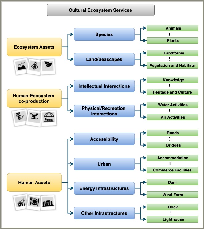
Figure 1: Hierarchy of Cultural Ecosystem Services (CES) classes representing all types of interactions between humans and protected areas (modified from CICES 5.2 https://cices.eu). The hierarchy includes three levels, Level-1 (orange color), Level-2 (blue color), Level-3 (green color).

Grouping social media images into a number of CES clusters is challenging for multiple reasons: i) the semantic meaning of several CES classes is broad and may refer to a huge number of different visual contents, ii) the large volume of the input images, iii) an important proportion of the input images maybe irrelevant to CES study, for example pictures that display text, screenshots and duplicated images. Several studies have tackled the task of clustering social media images into a small number of CES classes but all the proposed approaches rely either partially or entirely on manual intervention Moreno-Llorca et al. (2020), Yee & Carrasco (2024). Most relevant approaches in the field of computer vision are based on two steps, first a neural network is trained to learn inner representations from input images then in a second step the obtained visual embeddings are clustered using a carefully selected criteria Van Gansbeke et al. (2020).

Recent Large Vision Models (LVMs), also known as foundational models, encode a vast amount of visual representations that can be adapted to new vision tasks under the supervised learning, few-shot or zero-shot learning regimes. Similarly, Large Language Models (LLMs) process and generate natural language for various downstream tasks. Large Vision-Language Models (LVLMs) offer an additional adaptation method called prompting, enabling more effective task-specific customization. This study explores the potential of these large models—LVMs, LLMs, and LVLMs—in tackling the challenge of classifying large volumes of social media images into predefined categories, especially when the categories lack consistent visual patterns. As a case study, we address the sustainability issue of evaluating CES by mapping social media images into relevant classes.

2 Related work

The most related work to the present paper can be divided into two type of studies:

Cultural Ecosystem Services (CES) analysis: These studies focus mainly on understanding and mapping CES, which is still an open problem. The used methodologies to cluster social media images into a number of CES classes often involve human intervention in different parts of the process. For example, the authors in Moreno-Llorca et al. (2020) manually analyzed the entire volume of images posted on Flickr from the National park of Sierra Nevada, Granada, Spain. They intended to find CES classes that better match the visual content of the images and identified four classes: 1) Landscape and species, 2) recreation and sports, 3) culture and heritage, 4) others. When comparing the agreement between the assigned classes and results of an online survey for each image they found that the only consistent match is shown by the “Landscape and species” class. This disagreement can be explained by the use of an inappropriate semantic categories. In Yee & Carrasco (2024), the authors simplified the CES classes into three categories: biotic (interaction between human and biotic parts of nature), abiotic (interaction between human and abiotic parts of nature) and human-human (interaction between human and human). They first analyzed $87,090$ images using Microsoft’s Azure Computer Vision API and got a vector of $5,127$ pairs of labels and corresponding scores referring to diverse objects, living beings, and actions. Then they used a threshold of $50\%$ to filter non-relevant classes and applied a hierarchical agglomerative clustering that generated 430 clusters. In the last step they manually corrected and merged the obtained clusters into the three predefined classes.

Unsupervised image classification task: These studies focus mainly on automatizing the whole process of grouping a set of unlabeled images into semantic meaningful clusters. Existing approaches in this context are specific purpose models that follow one of these two dominant strategies: (1) In the first, the feature learning step and clustering are decoupled. For the representation learning, a self supervised learning pretext task is trained to predict transformations (e.g., rotation, colorization) or an instance discrimination process is applied using approaches such as SimCLR Chen et al. (2020). Afterwards, an offline clustering of the generated embedding performed. One of the most relevant works in this direction is SCAN Van Gansbeke et al. (2020). (2) The second approach is based on an end-to-end learning in which a CNN and clustering methods are coupled together. The losses of both methods are used to update the neural networks. Example of these approaches are DeepCluster Caron et al. (2019) and DEC Xie et al. (2016).

3 Background

Large Language Models:

Natural Language Natural Language Processing (NLP) has experienced two major breakthroughs that have paved the way for the development of powerful LLMs. The first was the introduction of the Transformer architecture, particularly the self-attention mechanism, in 2017 Vaswani (2017). The second was the rise of Self-Supervised Learning (SSL) algorithms Oord et al. (2018), which enabled the learning of meaningful representations from massive amounts of text without the need for labeled data. The combination of these two advancements has resulted in LLMs with significantly improved generalization across diverse NLP tasks. Among the most influential LLMs are: 1) BERT (Bidirectional Encoder Representations from Transformers), one of the first to achieve strong results across several NLP benchmarks; 2) RoBERTa (A Robustly Optimized BERT Pretraining Approach) Liu et al. (1907), an enhanced version of BERT with larger pre-training data; and 3) GPT-3 (Generative Pretrained Transformer 3) Brown (2020), the largest LLM with 175 billion parameters, excelling across various tasks and domains.

LLMs can be adapted to new NLP tasks through several methods: 1) Traditional fine-tuning or linear probing on specific labeled datasets to create specialized models, such as ChatGPT, which is based on a fine-tuned version of GPT-4. 2) Instruction Tuning, where the LLM is fine-tuned on a collection of NLP tasks presented as instructions, as seen in models like FLAN-T5 and FLAN-PaLM Chung et al. (2024). 3) Prompting, which enhances the model’s performance using few-shot learning or prompt engineering. 4) Retrieval-Augmented Generation (RAG) Lewis et al. (2020), which improves the model’s output by retrieving relevant information from an external specialized dataset. To reduce the cost of fine-tuning LLMs, distilled versions with fewer parameters, such as DistilBERT Sanh (2019), are commonly used.

Large Vision Models:

Inspired by the success of LLMs, LVMs are foundational models pretrained on vast amounts of images using self-supervised learning. These models generate a rich space of general-purpose features that can be adapted to new vision tasks through fine-tuning, few-shot, or zero-shot learning. Some of the most influential LVMs include CLIP Radford et al. (2021) and DINOv2 Oquab et al. (2023), with DINOv2 being regarded as state-of-the-art. DINOv2 was trained on curated and diverse datasets, enabling it to produce higher-quality features for a wide range of applications.

Large Vision Language Models:

Recently, the development of multimodal models has made significant strides by leveraging machine-generated instruction-following data. One of the earliest unified LVLMs is BLIP Li et al. (2022). The current state-of-the-art LVLM is LLaVA (Large Language and Vision Assistant), an end-to-end trained multimodal model that connects a vision encoder with a LLM for general-purpose visual and language understanding Liu et al. (2023). LLaVA utilizes the language-only GPT-4 to generate language-image instruction-following data. These models are generative, taking both image and text inputs to produce text outputs. LLaVA demonstrates strong zero-shot learning capabilities in tasks such as image-based chatting, image recognition via instructions, visual question answering, document understanding, image captioning, and more.

4 Data collection

We created the dataset named FLIPS (Flickr Images from Spanish Parks) as part of this study analyzing human interactions with nature. This dataset was compiled from images shared between 2015 and 2022 through Flickr social media platform, from various National parks across Spain.

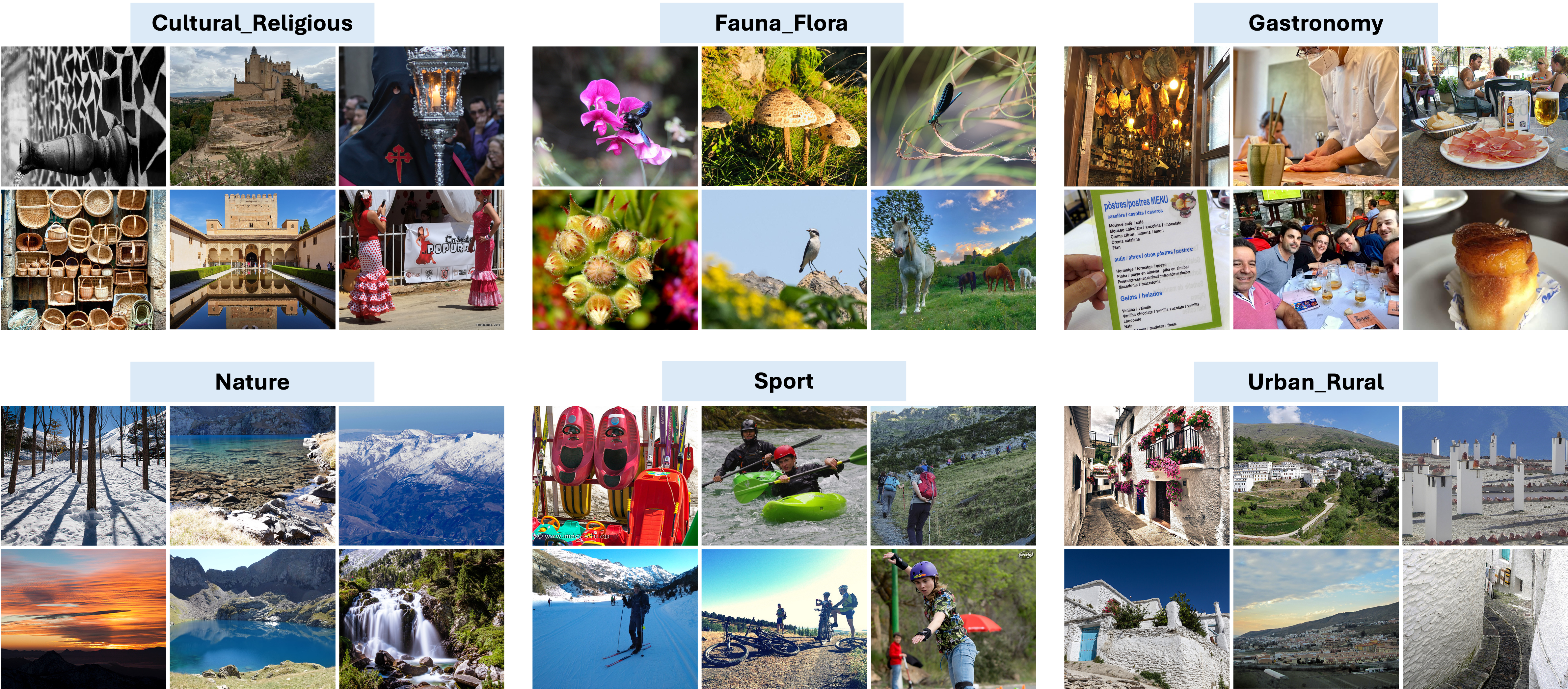
Figure 2: Six examples of each CES category.

To ensure high quality, we implemented a rigorous filtering process to remove any noisy images. The FLIPS dataset contains 960 images encompassing six CES classes: 1) Cultural-Religious, 2) Fauna-Flora, 3) Gastronomy, 4) Nature, 5) Sport, and 6) Urban-Rural. Each class contains 160 carefully curated images, providing a diverse representation of these themes.

5 Study design

To address the task of clustering unlabeled images into CES classes we propose analyzing five approaches that include state-of-the art large models in different stages of the processing. In particular, three approaches are based on LVLM to obtain the text embeddings from the input images and two approaches are based on LVM to obtain the visual embeddings (Figure 3). A total of eleven solutions were evaluated (Table 1). For a fair comparison, we used 5-fold cross-validation to evaluate the trainable models on the entire dataset, while for the untrained models, we directly applied them to the full FLIPS dataset.

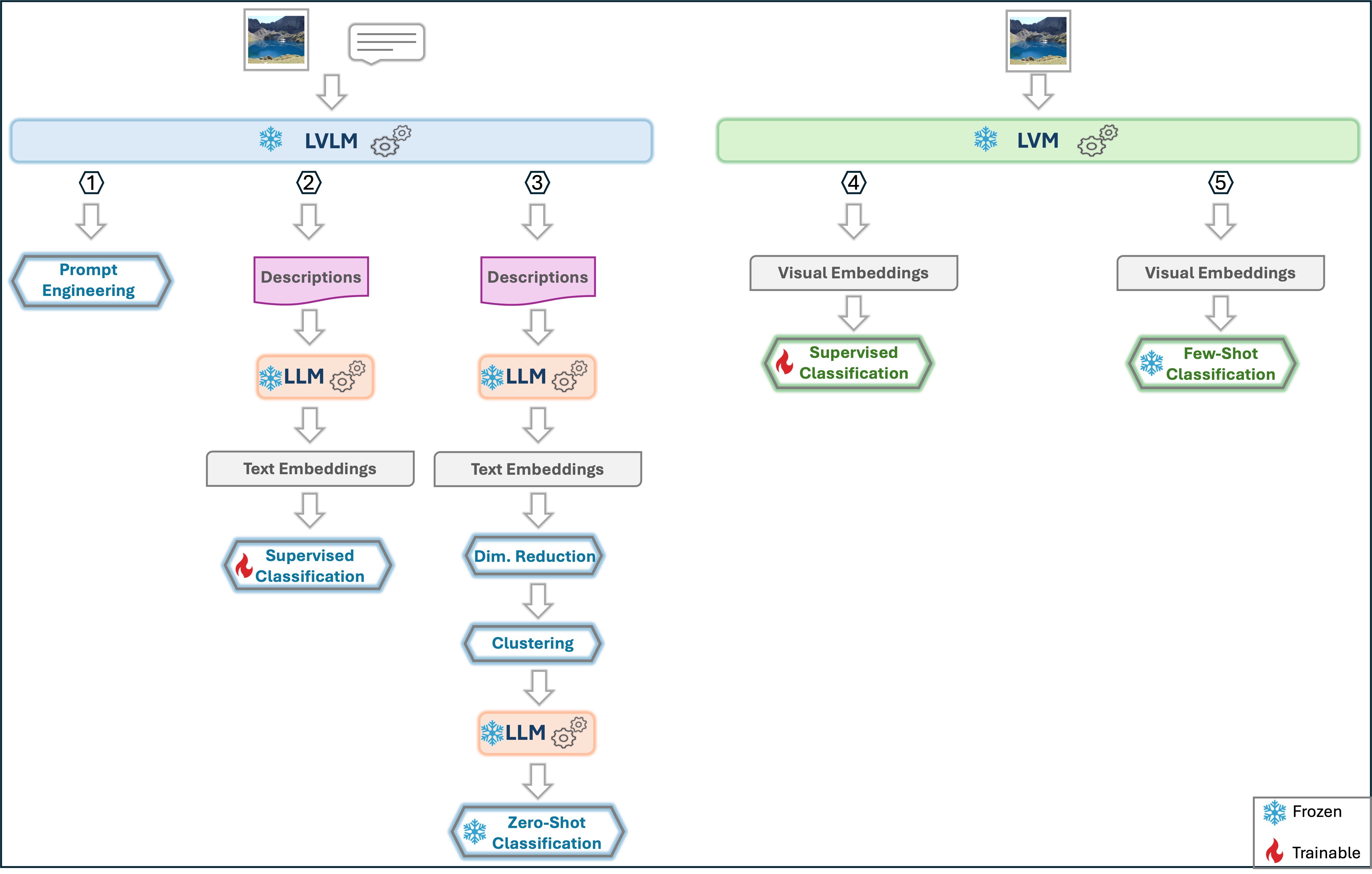
Figure 3: Visual illustration of the five evaluated approaches in this study.

Table 1: Description of the models used within each approach. FT stands for Fine-Tuning but actually refers to linear probing (i.e., only the last layer was trained). FSC refers to Few-Shot Classification.

Approach	Model Architecture
1	LLaVA-1.5
	GPT-4 (gpt-4o-mini)
2	LLaVA-1.5 + BERT-FT
	LLaVA-1.5 + DistilBERT-FT
	LLaVA-1.5 + RoBERTa-FT
	BLIP + BERT-FT
	BLIP + DistilBERT-FT
	BLIP + RoBERTa-FT
3	LLaVA-1.5 + SBERT + Flan-T5
4	DINO-FT
5	DINO-FSC

5.1 Approach 1: LVLM with prompt engineering

In this approach, we utilized a pretrained LVLM combined with prompt engineering (Figure 4). This method takes two inputs: the image to be classified and the prompt, and generates as output the category of the image. A post-processing step was applied to the model’s output to extract the class from the generated text. Two LVLM models were tested (Table 1): a public LLaVa-1.5 (Liu et al. 2024) and proprietary GPT-4 (gpt-4o-mini) (Achiam et al. 2023). Both models were applied directly to the data without additional training. Various simple and extended prompts were evaluated, the two prompts that provide the best results are shown in Table 2.

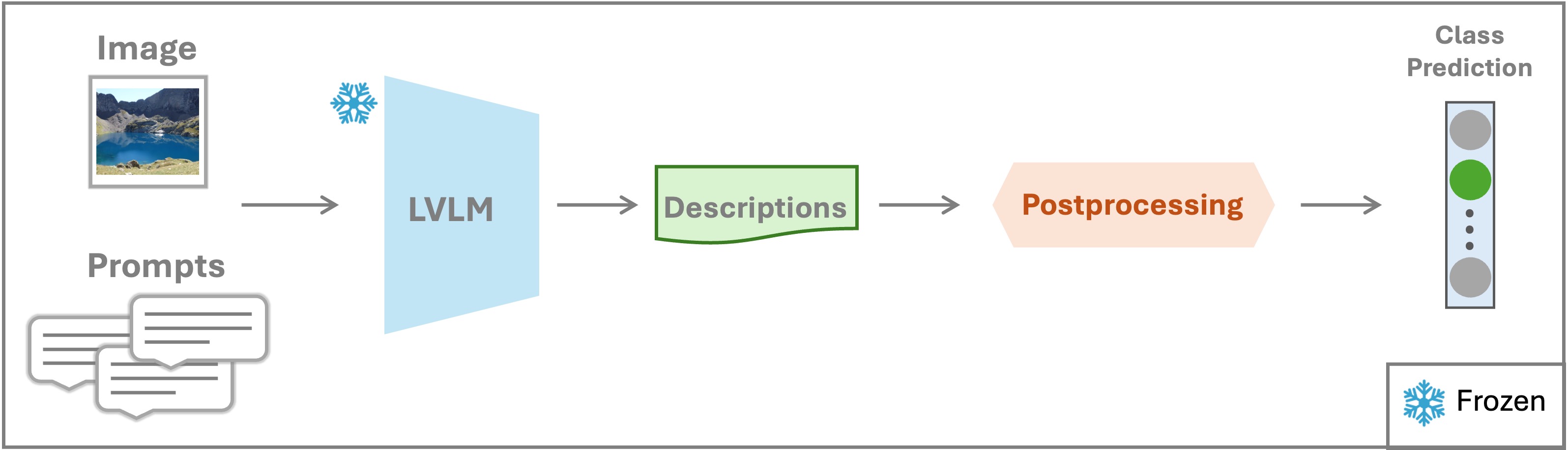
Figure 4: Visualization of approach (1) involving LVLM combined with prompt engineering.

Table 2: Description of the best two types of prompts used with LVLM-based approaches: (1) simple prompt and (2) extended prompt providing a definition for each class.

Prompt id	Prompt description
1	Classify the image into one of these categories: Cultural_Religious, Fauna_Flora, Gastronomy, Nature, Sports, or Urban_Rural.
2	Classify the image into one of these categories: Cultural_Religious, Fauna_Flora, Gastronomy, Nature, Sports, or Urban_Rural. The definitions for each category are as follows: Cultural_Religious: The image depicts religious symbols, cultural artifacts, traditions, ceremonies, or anything related to culture and belief systems. Fauna_Flora: The image features animals (fauna) or plants (flora) in any environment. Gastronomy: The image is related to food, cooking, culinary experiences, or dining. Nature: The image contains natural landscapes, such as mountains, rivers, forests, or other untouched environments. Sports: The image shows physical activities, competitions, or sports equipment related to athletic endeavors. Urban_Rural: The image captures cityscapes, villages, rural settings, buildings, or any human-made environments.

5.2 Approach 2: LVLM with supervised classification of LLM

In this approach, we utilized a pretrained LVLM in conjunction with a pretrained LLM (Figure 5). The process unfolds as follows: (1) We employed the LVLM to generate descriptions for each image, evaluating two advanced LVLM architectures: LLaVA-1.5 and BLIP (Li et al. 2022). (2) We then used the LLM to generate text embeddings for these descriptions, experimenting with three different LLM architectures: BERT (Devlin 2018), DistilBERT (Sanh 2019), and RoBERTa (Liu et al. 2019). (3) Finally, we trained the head-layer, also known as linear probing, of the LLM to classify the descriptions into our predefined categories.

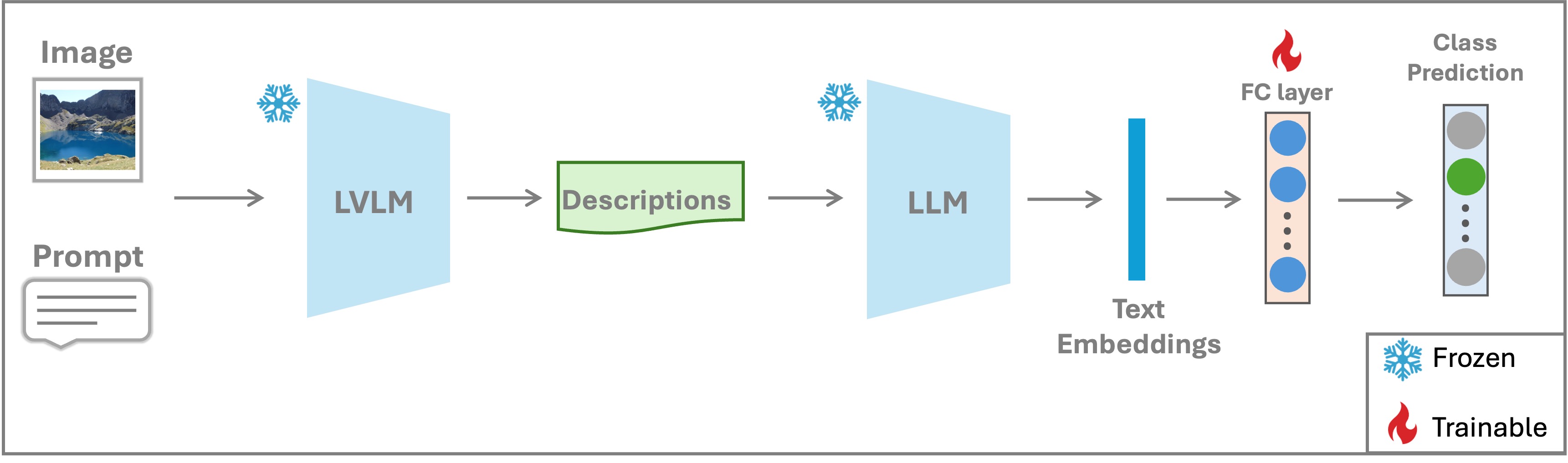
Figure 5: Visualization of approach (2) combining LVLM with finetuned LLM.

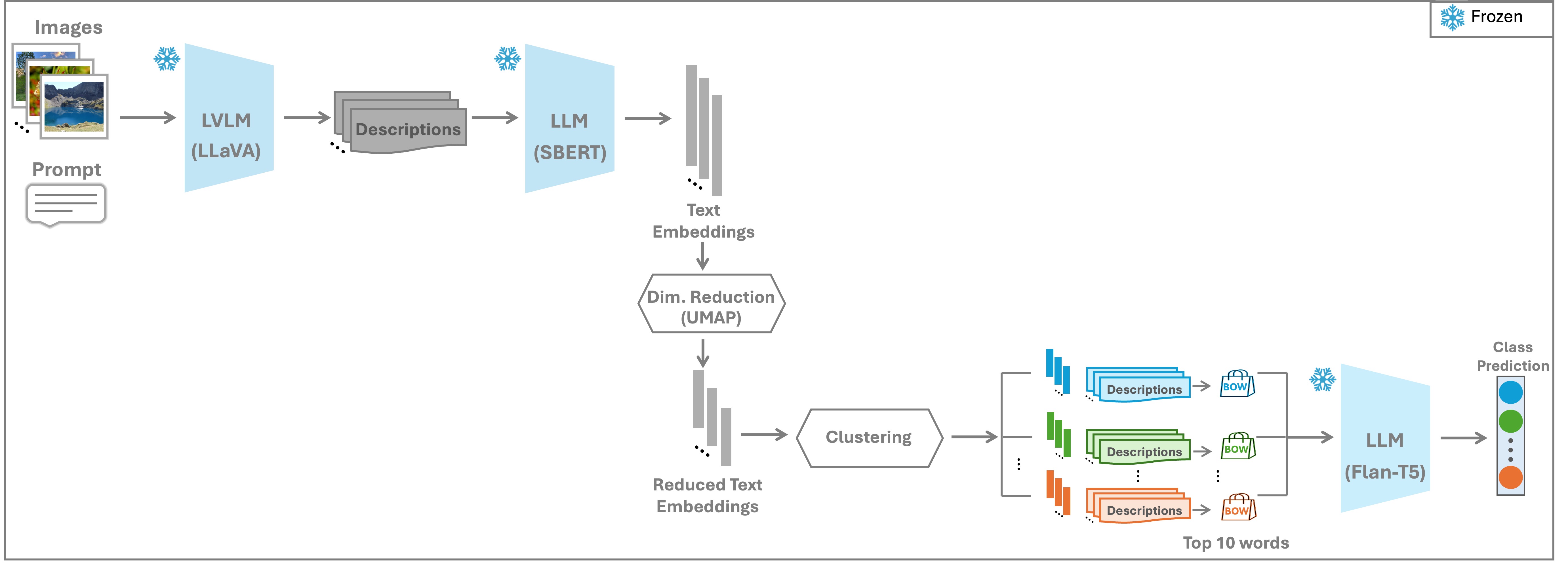
Figure 6: Visualization of approach (3) combining LVLM and LLMs with dimensionality reduction, clustering, and zero-shot classification.

5.3 Approach 3: LVLM and LLMs with dimensionality reduction, clustering, and zero-shot classification

In this approach, we leveraged a pretrained LVLM alongside with a pretrained LLMs, dimensionality reduction model, clustering model, and zero-shot classification (Figure 6). The process is as follows: (1) We used the pretrained LVLM LLaVA-1.5 to generate descriptions for each image. (2) These descriptions were then converted into text embeddings using the pretrained LLM Sentence-BERT (SBERT) (Reimers 2019). (3) To mitigate the curse of high dimensionality, we applied UMAP (McInnes et al. 2018), a state-of-the-art dimensionality reduction model, to project these embeddings into a lower-dimensional space while preserving both local and global data structure. (4) Clustering were performed on the reduced embeddings using two different clustering models, KMeans and HDBSCAN (McInnes et al. 2017). (5) For each cluster, we now have a collection of image descriptions. We tokenized these descriptions and then identified the ten most representative words based on Term Frequency (TF) and Inverse Document Frequency (IDF) scores. These top ten words constitute the Bag of Words (BOW) for each cluster. (6) Finally, we used another pretrained LLM, Flan-T5 (Chung et al. 2024), in a zero-shot classification setting to map each cluster to our predefined classes based on the generated BOW per cluster and a specific prompt structure. Flan-T5, having been fine-tuned with instruction-based learning across various tasks, is well-suited for zero-shot text classification (Mann et al. 2020).

5.4 Approach 4: LVM with supervised classification head

In this approach, we employed a pretrained LVM combined with a supervised classifier (Figure 7). The method ingested an input image and used a pretrained LVM to generate visual embeddings. These embeddings were then processed by a fully connected (FC) layer to predict the class with the highest probability. Only the classifier head was trained, while the backbone remained frozen. For this approach, we used the state-of-the-art DINOv2 LVM model (Oquab et al. 2023).

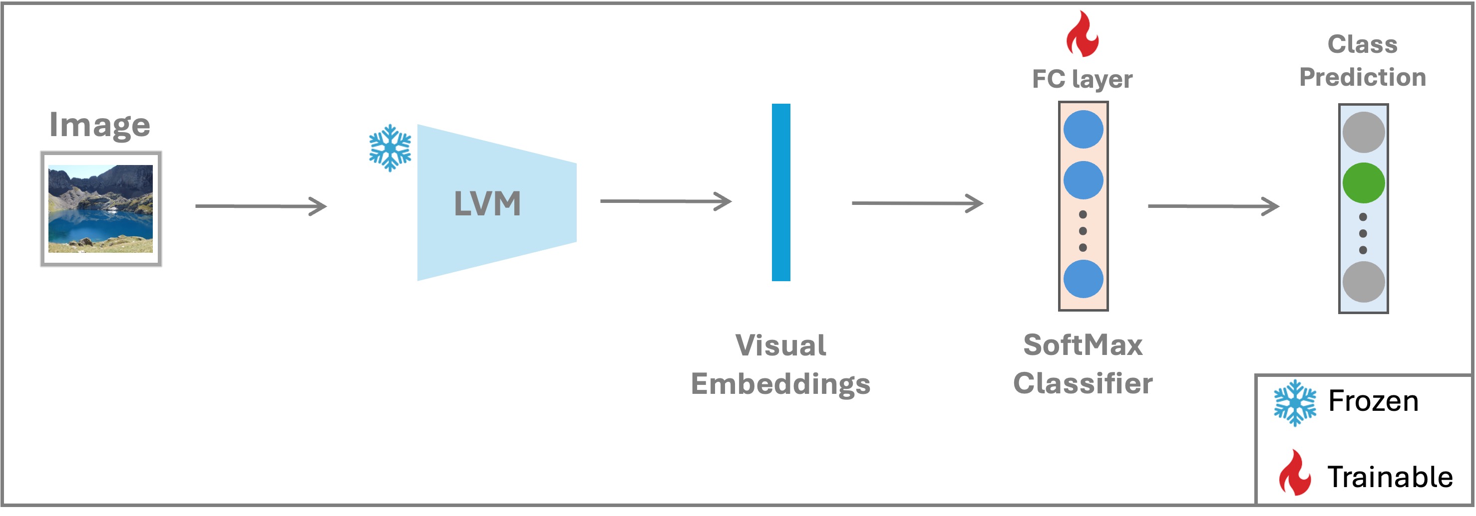
Figure 7: Visualization of approach (4) involving LVM (DINOv2) combined with a supervised classifier.

5.5 Approach 5: LVM with few-shot classification

In this approach, we utilized a pretrained LVM in conjunction with few-shot classification (Figure 8). We used two data partitions: (1) a support set with different configurations of shots, ranging from 1 to 10, and (2) a query set consisting of all the remaining samples that do not belong to the support set. To assess the model’s stability concerning the support set samples, we generated 30 random support sets for each shot configuration and computed the average model performance. The method operates as follows: (1) we created a support set containing six classes with a specified number of shots per class; (2) we applied the LVM to generate visual embeddings for both the support and query set samples; (3) we computed a prototype for each class in the support set by averaging the embeddings of the samples in that class; (4) we compared the embedding vector of the query sample with the prototypes’ embeddings using a cosine similarity function normalized by the Softmax function; (5) we assigned to the query sample the class label of the closest prototype (i.e., the one with the highest Softmax value). For this approach, we employed the DINOv2 LVM model.

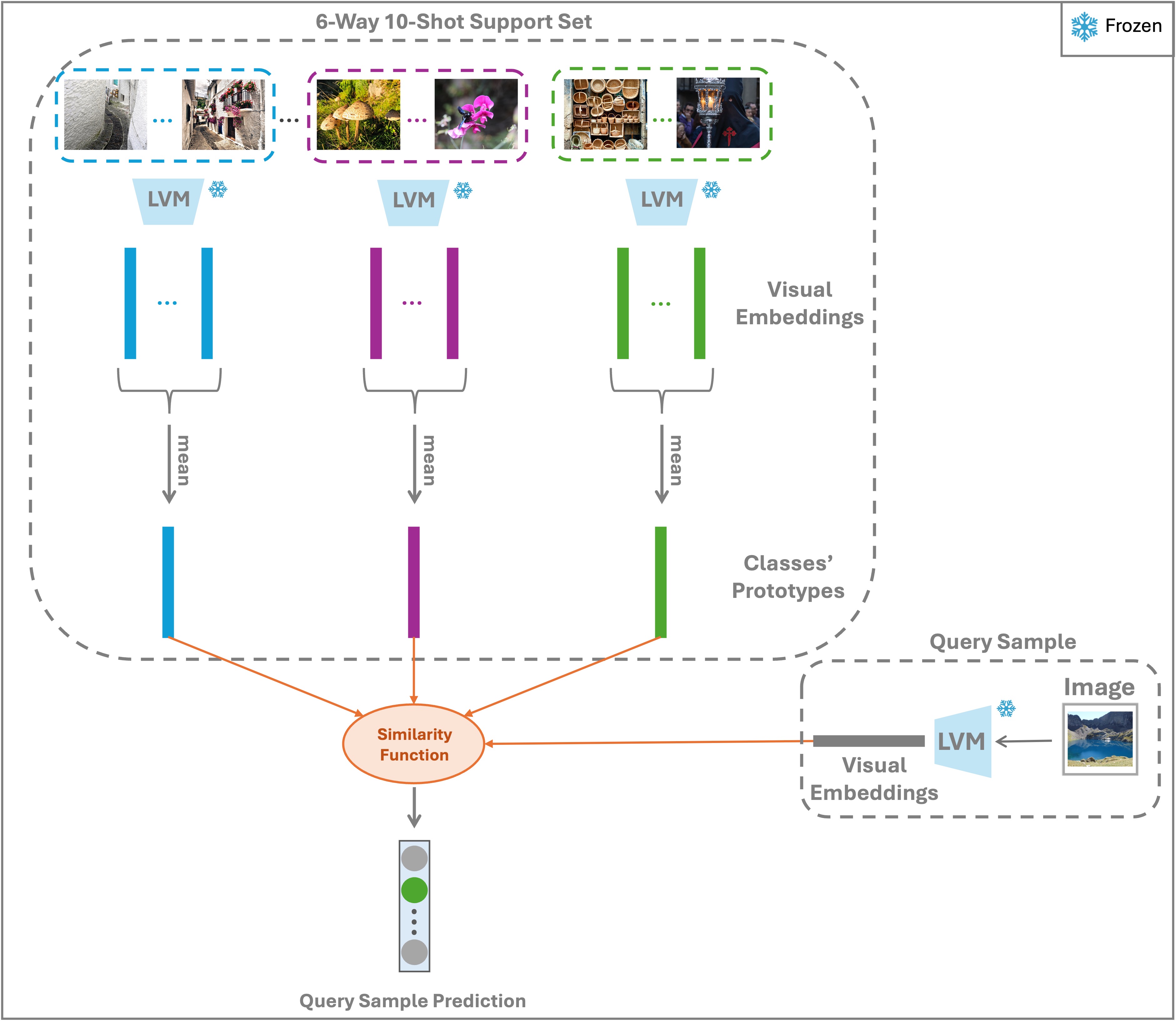
Figure 8: Visualization of approach (5) involving LVM (DINOv2) combined with Few-Shot classification.

6 Results and discussion

In this section, we present the optimal results for each approach and then provide a comparison of all approaches against one another.

Approach 1

Table 3 summarizes the results of applying the models from approach (1), specifically LLaVA-1.5 and GPT-4, using two different prompts: a simple prompt (prompt 1) and an extended prompt (prompt 2). LLaVA-1.5 achieved its highest accuracy of 84.48% with prompt 1, compared to 80.10% with prompt 2. In contrast, GPT-4 performed best with prompt 2, reaching 88.02% accuracy, slightly higher than the 87.92% with prompt 1. Overall, GPT-4 outperformed LLaVA-1.5, with an accuracy of 88.02% versus 84.48%.

Table 3: Test results of the models used in approach (1) with two different prompts: simple prompt (prompt 1) and extended prompt (prompt 2).

Approach	Model Architecture	Prompt	Precision	Recall	Accuracy
1	LLaVA-1.5	1	87.02	84.48	84.48
		2	86.05	80.10	80.10
	GPT-4 (gpt-4o-mini)	1	90.41	87.92	87.92
		2	90.15	88.02	88.02

Approach 2

Table 4 presents the results of the models used in approach (2), which involve two LVLMs, LLaVA-1.5 and BLIP, combined with the linear probing of three different LLM architectures: BERT, DistilBERT, and RoBERTa. Across all used LLM architectures, LLaVA-1.5 consistently outperformed BLIP. The highest overall accuracy was achieved with the LLaVA-1.5+DistilBERT-FT combination, reaching 95.00%, compared to 88.02% for BLIP+DistilBERT-FT.

Table 4: Test results of the models used in approach (2). FT stands for Fine-Tuning but actually refers to linear probing (i.e., only the last layer was trained).

Approach	Model Architecture	Precision	Recall	Accuracy
2	LLaVA-1.5 + BERT-FT	94.95	94.79	94.79
	LLaVA-1.5 + DistilBERT-FT	95.08	95.00	95.00
	LLaVA-1.5 + RoBERTa-FT	94.92	94.79	94.79
	BLIP + BERT-FT	88.73	88.65	88.65
	BLIP + DistilBERT-FT	88.24	88.02	88.02
	BLIP + RoBERTa-FT	88.49	88.23	88.23

Approach 3

Table 5 presents the results of the models used in approach (3), which combines the LVLM LLaVA-1.5 with two LLMs, SBERT and Flan-T5, utilizing dimensionality reduction, clustering, and zero-shot classification. This table showcases the results obtained from two different clustering algorithms: KMeans and HDBSCAN. The best performance was achieved using KMeans, reaching an accuracy of 72.60%, compared to 70.73% obtained with HDBSCAN. However, HDBSCAN had the highest precision at 85.45%, significantly outperforming KMeans, which achieved 66.08%.

Table 5: Test results of the models used in approach (3).

Approach	Model Architecture	Clustering model	Precision	Recall	Accuracy
3	LLaVA-1.5 + SBERT + Flan-T5	KMeans	66.08	72.60	72.60
		HDBSCAN	85.45	70.73	70.73

Approach 4

Table 6 displays the results of the models used in approach (4), which consists in training the classifier head of the LVM DINOv2 using visual embeddings generated from three different ViT backbone architectures with varying computational complexities: S (small size), B (base size), and L (large size). The best performance was achieved with the large ViT model architecture, ViT-L/14, which attained an accuracy of 97.08%.

Table 6: Test results of the models used in approach (4). FT stands for Fine-Tuning but actually refers to linear probing (i.e., only the last layer was trained).

Approach	Model Architecture	Backbone	Precision	Recall	Accuracy
4	DINO-FT	ViT-S/14	94.77	94.58	94.58
		ViT-B/14	96.85	96.77	96.77
		ViT-L/14	97.20	97.08	97.08

Approach 5

Table 7 presents the results of the models used in approach (5) combining the LVM DINOv2 with three different ViT backbone architectures using 10-shot classification. The optimal results were obtained with ViT-S/14 with an accuracy of 83.99% compared to 79.96% with ViT-L/14. Figure 9 displays the test results of running the backbone ViT-S/14 using different shots ranging from 1 to 10. Each configuration of shot was run using 30 different random support sets. The highest average accuracy was obtained using 10 shots.

Table 7: Test results of the models used in approach (5) using 10-shot classification setting. FSC refers to Few-Shot Classification.

Approach	Model Architecture	Backbone	Precision	Recall	Accuracy
5	DINO-FSC (10 shots)	ViT-S/14	83.56	83.54	83.99
		ViT-B/14	80.61	80.40	80.67
		ViT-L/14	79.89	79.62	79.96

Figure 9: Average accuracy over different query sets generated through the creation of 30 random support set samples for varying shot counts from 1 to 10, using the backbone ViT-S/14.

Comparison of all approaches

Table 8 summarizes the results of all the models utilized under the five different approaches for recognizing CES from social media images, highlighting the best configurations. In general, the models implemented under approach (1), (2), (4), and (5) provide better results than approach (3). The best results were obtained under the supervised setting using the LVM DINOv2 achieving a top accuracy of 97.08% and LLaVA-1.5 combined with the fine-tuned LLM DistilBERT with accuracy 95%. The second performing models were under the unsupervised setting, namely GPT-4 with 88.02% and LLaVA-1.5 with 84.48% accuracy. It is noteworthy to mention that these approaches do not require a strong programming or AI background.

The class-specific results in Table 9 indicate that DINO-FT achieved the highest accuracy in classifying the categories Cultural-Religious and Urban-Rural, with 97.50% and 98.12%, respectively. GPT-4 excelled in classifying the Gastronomy and Nature categories, reaching 100% and 99.38% accuracy, respectively. Both models performed equally well in classifying the Fauna-Flora category, with 98.12% accuracy. For the Sports category, the fine-tuned LLaVA-1.5+DistilBERT and LLaVA-1.5+SBERT+Flan-T5 achieved the best results, both with an accuracy of 97.50%. According to the class-specific results, each model can be used to recognize a specific class and/or classes.

Table 8: Test results of the different models used in this study. The best results in each approach are underlined. The top results over all approaches are highlighted in bold. FT stands for Fine-Tuning but actually refers to linear probing (i.e., only the last layer was trained). FSC refers to Few-Shot Classification.

Approach	Model Architecture	Precision	Recall	Accuracy
1	LLaVA-1.5	87.02	84.48	84.48
	GPT-4 (gpt-4o-mini)	90.15	88.02	88.02
2	LLaVA-1.5 + BERT-FT	94.95	94.79	94.79
	LLaVA-1.5 + DistilBERT-FT	95.08	95.00	95.00
	LLaVA-1.5 + RoBERTa-FT	94.92	94.79	94.79
	BLIP + BERT-FT	88.73	88.65	88.65
	BLIP + DistilBERT-FT	88.24	88.02	88.02
	BLIP + RoBERTa-FT	88.49	88.23	88.23
3	LLaVA-1.5 + SBERT + Flan-T5 (KMeans)	66.08	72.60	72.60
4	DINO-FT (ViT-L/14)	97.20	97.08	97.08
5	DINO-FSC (ViT-S/14 - 10 shots)	83.56	83.54	83.99

Table 9: Class-specific test results of the different models used in this study. FT stands for Fine-Tuning but actually refers to linear probing (i.e., only the last layer was trained). FSC refers to Few-Shot Classification.

Approach	Model Architecture	Cultural Religious	Fauna Flora	Gastronomy	Nature	Sports	Urban Rural
1	LLaVA-1.5	96.25	94.38	99.38	98.75	68.75	49.38
	GPT-4 (gpt-4o-mini)	76.25	98.12	100.00	99.38	62.50	91.88
2	LLaVA-1.5 + BERT-FT	91.25	98.12	98.75	95.62	96.25	90.00
	LLaVA-1.5 + DistilBERT-FT	89.38	97.50	96.88	93.75	97.50	88.12
	LLaVA-1.5 + RoBERTa-FT	93.12	96.25	98.75	94.38	96.88	89.38
	BLIP + BERT-FT	84.38	95.62	98.12	85.62	91.88	80.00
	BLIP + DistilBERT-FT	84.38	91.88	96.88	85.00	91.88	78.12
	BLIP + RoBERTa-FT	90.00	96.25	97.50	82.50	90.62	76.88
3	LLaVA-1.5 + SBERT + Flan-T5 (KMeans)	0	66.88	98.12	93.65	97.50	79.38
4	DINO-FT (ViT-L/14)	97.50	98.12	98.12	98.12	93.12	97.50
5	DINO-FSC (ViT-S/14 - 10 shots)	79.79	76.80	94.06	83.13	77.25	90.23

7 Conclusion

This work investigated the challenge of mapping social media images into a set of CES categories by leveraging the latest advancements in large models, including LVLM, LVM, and LLM. We proposed, analyzed, and compared multiple approaches that utilized one or a combination of these models to address this problem.

Our experiments demonstrated that the best performance came from supervised approaches, specifically the fine-tuned LVM DINOv2 and the LVLM LLaVA-1.5 combined with a fine-tuned LLM. Unsupervised approaches based on LVLMs followed, with the proprietary GPT-4 model leading, followed by the public LLaVA-1.5 model. Additionally, the LVM DINOv2 under a 10-shot learning setup also delivered competitive results, comparable to those of the LVLM LLaVA-1.5.

Overall, our study highlights the potential of large models, with LVLMs standing out for ease of use and LVMs for their performance when fine-tuned. As future work we plan to explore applying these approaches to finer-grained CES categories.

Declaration of Competing Interest

The authors declare that they have no known competing financial interests or personal relationships that could have appeared to influence the work reported in this paper.

Data availability

Data will be made available to the public in Zenodo repository after the acceptation of the paper.

References

- Achiam et al. (2023) Achiam, J., Adler, S., Agarwal, S., Ahmad, L., Akkaya, I., Aleman, F. L., Almeida, D., Altenschmidt, J., Altman, S., Anadkat, S. et al. (2023). Gpt-4 technical report. arXiv preprint arXiv:2303.08774, .
- Brown (2020) Brown, T. B. (2020). Language models are few-shot learners. arXiv preprint arXiv:2005.14165, .
- Caron et al. (2019) Caron, M., Bojanowski, P., Mairal, J., & Joulin, A. (2019). Unsupervised pre-training of image features on non-curated data. In Proceedings of the IEEE/CVF International Conference on Computer Vision (pp. 2959–2968).
- Chen et al. (2020) Chen, T., Kornblith, S., Norouzi, M., & Hinton, G. (2020). A simple framework for contrastive learning of visual representations. In International conference on machine learning (pp. 1597–1607). PMLR.
- Chung et al. (2024) Chung, H. W., Hou, L., Longpre, S., Zoph, B., Tay, Y., Fedus, W., Li, Y., Wang, X., Dehghani, M., Brahma, S. et al. (2024). Scaling instruction-finetuned language models. Journal of Machine Learning Research, 25, 1–53.
- Devlin (2018) Devlin, J. (2018). Bert: Pre-training of deep bidirectional transformers for language understanding. arXiv preprint arXiv:1810.04805, .
- Gatzweiler et al. (2024) Gatzweiler, F. W., Hagedorn, K., & Pascual, U. (2024). Biodiversity and cultural ecosystem services. In S. M. Scheiner (Ed.), Encyclopedia of Biodiversity (Third Edition) (pp. 290–299). Oxford: Academic Press. (Third edition ed.). doi:https://doi.org/10.1016/B978-0-12-822562-2.00145-6.
- Havinga et al. (2023) Havinga, I., Marcos, D., Bogaart, P., Massimino, D., Hein, L., & Tuia, D. (2023). Social media and deep learning reveal specific cultural preferences for biodiversity. People and Nature, 5, 981–998.
- Lewis et al. (2020) Lewis, P., Perez, E., Piktus, A., Petroni, F., Karpukhin, V., Goyal, N., Küttler, H., Lewis, M., Yih, W.-t., Rocktäschel, T. et al. (2020). Retrieval-augmented generation for knowledge-intensive nlp tasks. Advances in Neural Information Processing Systems, 33, 9459–9474.
- Li et al. (2022) Li, J., Li, D., Xiong, C., & Hoi, S. (2022). Blip: Bootstrapping language-image pre-training for unified vision-language understanding and generation. In International conference on machine learning (pp. 12888–12900). PMLR.
- Lingua et al. (2022) Lingua, F., Coops, N. C., & Griess, V. C. (2022). Valuing cultural ecosystem services combining deep learning and benefit transfer approach. Ecosystem Services, 58, 101487.
- Liu et al. (2023) Liu, H., Li, C., Li, Y., & Lee, Y. J. (2023). Improved baselines with visual instruction tuning.
- Liu et al. (2024) Liu, H., Li, C., Li, Y., & Lee, Y. J. (2024). Improved baselines with visual instruction tuning. In Proceedings of the IEEE/CVF Conference on Computer Vision and Pattern Recognition (pp. 26296–26306).
- Liu et al. (2019) Liu, Y., Ott, M., & Goyal, N. (2019). Jingfei du, mandar joshi, danqi chen, omer levy, mike lewis, luke zettlemoyer, and veselin stoyanov. 2019. roberta: A robustly optimized bert pretraining approach. arXiv preprint arXiv:1907.11692, 1, 3–3.
- Liu et al. (1907) Liu, Y., Ott, M., Goyal, N., Du, J., Joshi, M., Chen, D., Levy, O., Lewis, M., Zettlemoyer, L., & Stoyanov, V. (1907). Roberta: A robustly optimized bert pretraining approach. arxiv [preprint](2019). arXiv preprint arXiv:1907.11692, .
- Mann et al. (2020) Mann, B., Ryder, N., Subbiah, M., Kaplan, J., Dhariwal, P., Neelakantan, A., Shyam, P., Sastry, G., Askell, A., Agarwal, S. et al. (2020). Language models are few-shot learners. arXiv preprint arXiv:2005.14165, 1.
- McInnes et al. (2017) McInnes, L., Healy, J., Astels, S. et al. (2017). hdbscan: Hierarchical density based clustering. J. Open Source Softw., 2, 205.
- McInnes et al. (2018) McInnes, L., Healy, J., & Melville, J. (2018). Umap: Uniform manifold approximation and projection for dimension reduction. arXiv preprint arXiv:1802.03426, .
- Moreno-Llorca et al. (2020) Moreno-Llorca, R., Méndez, P. F., Ros-Candeira, A., Alcaraz-Segura, D., Santamaría, L., Ramos-Ridao, Á. F., Revilla, E., Bonet-García, F. J., & Vaz, A. S. (2020). Evaluating tourist profiles and nature-based experiences in biosphere reserves using flickr: Matches and mismatches between online social surveys and photo content analysis. Science of the Total Environment, 737, 140067.
- Oord et al. (2018) Oord, A. v. d., Li, Y., & Vinyals, O. (2018). Representation learning with contrastive predictive coding. arXiv preprint arXiv:1807.03748, .
- Oquab et al. (2023) Oquab, M., Darcet, T., Moutakanni, T., Vo, H., Szafraniec, M., Khalidov, V., Fernandez, P., Haziza, D., Massa, F., El-Nouby, A. et al. (2023). Dinov2: Learning robust visual features without supervision. arXiv preprint arXiv:2304.07193, .
- Radford et al. (2021) Radford, A., Kim, J. W., Hallacy, C., Ramesh, A., Goh, G., Agarwal, S., Sastry, G., Askell, A., Mishkin, P., Clark, J. et al. (2021). Learning transferable visual models from natural language supervision. In International conference on machine learning (pp. 8748–8763). PMLR.
- Reimers (2019) Reimers, N. (2019). Sentence-bert: Sentence embeddings using siamese bert-networks. arXiv preprint arXiv:1908.10084, .
- Sanh (2019) Sanh, V. (2019). Distilbert, a distilled version of bert: Smaller, faster, cheaper and lighter. arXiv preprint arXiv:1910.01108, .
- Van Gansbeke et al. (2020) Van Gansbeke, W., Vandenhende, S., Georgoulis, S., Proesmans, M., & Van Gool, L. (2020). Scan: Learning to classify images without labels. In European conference on computer vision (pp. 268–285). Springer.
- Vaswani (2017) Vaswani, A. (2017). Attention is all you need. Advances in Neural Information Processing Systems, .
- Xie et al. (2016) Xie, J., Girshick, R., & Farhadi, A. (2016). Unsupervised deep embedding for clustering analysis. In International conference on machine learning (pp. 478–487). PMLR.
- Yee & Carrasco (2024) Yee, T. B. L., & Carrasco, L. R. (2024). Applying deep learning on social media to investigate cultural ecosystem services in protected areas worldwide. Scientific Reports, 14, 13700.