Comprehensive Performance Modeling and System Design Insights for Foundation Models

Abstract

Generative AI, in particular large transformer models, are increasingly driving HPC system design in science and industry. We analyze performance characteristics of such transformer models and discuss their sensitivity to the transformer type, parallelization strategy, and HPC system features (accelerators and interconnects). We utilize a performance model that allows us to explore this complex design space and highlight its key components. We find that different transformer types demand different parallelism and system characteristics at different training regimes. Large Language Models are performant with 3D parallelism and amplify network needs only at pre-training scales with reduced dependence on accelerator capacity and bandwidth. On the other hand, long-sequence transformers, representative of scientific foundation models, place a more uniform dependence on network and capacity with necessary 4D parallelism. Our analysis emphasizes the need for closer performance modeling of different transformer types keeping system features in mind and demonstrates a path towards this. Our code is available as open-source at [1].

I Introduction

Transformers [2] have enabled state-of-the-art results across several disciplines including natural language processing (NLP) [3, 4, 5, 6, 7], computer vision (CV) [8, 9, 10] and scientific machine learning (SciML) [11, 12, 13]. These models are expected to form the foundation for machine learning models across various disciplines, owing to their impressive scaling properties with data and model sizes [14]. Large-language models (LLMs) are the most well-known foundation models such as GPT models [15] with model sizes ranging to a trillion parameters [16, 17] and are trained at large supercomputers at significant cost. For instance, the 1 trillion parameter Megatron GPT model was trained on 450 billion tokens, using 3072 Nvidia A100 GPUs, and requires 84 days [16]. Today, this cost is amplified by the need to train such models across multi-disciplinary domains in science—there is substantial effort to develop multiple foundation models for applications such as weather and climate modeling [12, 13], earthquake modeling [18], fluid dynamics simulations [19], protein structure predictions [20, 21], material sciences [22], and more. Each domain introduces its own design considerations for transformer models, as well as unique input data scales (resolutions) and training methodologies. This strongly motivates the need to theoretically analyze and understand the costs and bottlenecks associated with training different transformer types at scale and their relationship with the underlying system hardware. Our goal is to systematically present a framework for modeling the transformer performance and utilize this to explore optimal training strategies of the transformer at different system scales, transformer model regimes, and underlying system (hardware and network) characteristics.

Building this analytical performance model is challenging because the design space is extremely large—one must model system configurations like device (GPUs) memory capacity and bandwidth, compute speeds, and (multi-bandwidth) network configurations, along with various parallelization strategies that grow exponentially with model and system size. The latter is especially complex because large transformers typically demand multiple forms of parallelism simultaneously, with each introducing its own set of trade-offs. Data parallelism is effective but insufficient for large models (and input resolutions) and not memory-efficient, tensor parallelism [23, 16] reduces memory utilization at the cost of increased communication, and pipeline parallelism [16] can reduce communication costs at the expense of idle (bubble) times. Overextending any one strategy can introduce substantial costs and they must be carefully balanced. We present and utilize an analytic parameterized performance model that searches the combinatorial design space and discovers this balance as a function of the deep learning model and system configuration. While our performance model is applicable to any accelerator system with tiers of network performance, we present detailed performance analysis for commonly used system architectures with current and near-future NVIDIA GPU hardware with high-bandwidth memory (HBM) on device, a fast interconnect domain (compute node) with NVLink interconnect between GPUs (facilitated through NVSwitch [24]), a slow interconnect domain (inter-node) InfiniBand (or SlingShot/ethernet) for GPUs, and communication collectives through NCCL [25]. Our contributions are as follows:

1. Framework for building an AI performance model. We systematically outline the strategy to model the various components of the transformer architecture. We model the different operations (activation-weights, activation-activation matrix multiplies, vector operations) and highlight how parallelization strategies and other optimizations change the nature of these operations (arithmetic intensities, memory usage, communication times and other inefficiencies, see §III). Defining a configuration as the parallelization strategy along with other possible optimizations, the framework identifies an optimal configuration through a brute-force search of all possible configurations and selects the one with minimum training time, making this exploration orders of magnitude faster than experimentation.

2. Assessment of varying needs of SciML and NLP models. We assess two different transformer versions: GPT3-1T (1 trillion parameter GPT3 model) representing an LLM foundation model and ViT, a long-sequence vision transformer that represents transformers in science, where long sequences are necessary to process high-resolution inputs, designed to capture crucial fine-scaled physical features [26, 27, 13]. We then conduct the below analyses for both models independently, aiming to distinguish their training needs at different scales and across different systems.

3. Identifying optimal parallelism and training bottlenecks. We include data parallelism, tensor parallelism (1D), and pipeline parallelism that are part of standard LLM training in our framework and demonstrate their individual trade-offs in training times (see Fig. 1, 2). We further include two different 2D versions of tensor parallelism (with additional sequence parallelism or SUMMA [28] matrix multiplies) to demonstrate their impact on training the different model classes (see Fig. 3, 4(b)). We show that while 1D tensor parallelism is performant for GPT3-1T (see Fig. 5(a)), 2D tensor parallelism is necessary for ViT and depicts different training bottlenecks than the 1D version (see Fig. 4(b)). For both models, 2D tensor parallelism is optimal.

4. Performance impact of a fast network domain and GPU generations. We analyze the impact of the size of NVSwitch (NVS) that provides high bandwidth between all GPUs in that domain (node), with cross-domain (inter-node) slower InfiniBand (IB). We show that placement of GPUs from different parallelization groups within NVS domain introduces different optimal configurations identified at different NVS sizes (see discussions around Fig. 2, 3). Further, we show that, depending on the type of model, NVS size effects show up at different scales, lending to different requirements for pre-training and fine-tuning jobs. GPT3-1T only requires large NVS domain sizes at large training scale, needed for pre-training. However, a moderate scale fine-tuning may not require this. We also notice that HBM capacity is less important at scale for this model (see Fig. 5). The ViT however shows contrasting results with a more uniform dependence on NVS domain sizes and HBM capacity, owing to its massive sequence lengths (see Fig. 5(b)). Both models show good performance with alternate low bandwidth/high capacity memory, which may help alleviate the dependence on NVS through increased capacity. We also show the performance improvements with different GPU generations (A100, H200, B200) for each model which can be attributed to increased tensor core and network bandwidth performance.

II Related Work

We focus on analytical modeling and do not consider lower-level hardware simulation studies aimed at precise modeling of GPUs or the network since they are very costly for a full design space search. Our parallelization strategies are modeled based on tensor parallelism (1D [23], multi-dimensional [29, 30, 31]), pipeline parallelism [16] and ZeRO [32]. An early performance model exploring the design space is [16] for training a version of GPT3-1T. They do not conduct an automatic exploration of the design space but instead develop heuristic takeaways by focusing on a subset of the design space through analytical formulae. One of the first attempts at an automatic exploration and selection of parallelism strategies was by [33], where given a cluster mesh, the package compiles the computation graph into a distributed sharded graph, but is not network topology aware. In [34], they developed an open-source package that integrates an auto-parallelism feature that searches over the design space. Such auto-parallel approaches provide the user with a ready distributed training solution at the cost of hiding the rationale behind the specific strategy adopted. Calculon [35] was the first approach in building an in-depth, analytical performance model of both the LLM and the system for a high level and a unified exploration of the design space of hardware and software. Through the performance model, the authors identified new configurations that show better efficiencies for LLMs. However, their model is restricted to LLMs and analysis fixed to a system type. They only include 1D tensor parallelism (performant for LLMs), do not consider the effects of NVS domains on IB bandwidths and optimal strategies regarding placement of GPUs on the NVS domain, and do not include details on the diverse components of the underlying performance model, making it challenging to expand upon. We build on the Calculon approach and expose the different performance modeling components along with several modifications that include NVS domain size effects, GPU placement, 2D tensor parallelism variants (necessary for other model types) and conduct an extended analysis on different model types, GPU, and network characteristics.

III Methods

Denoting $b$ as batch size, $l$ as sequence length, $e$ as embedding dimension, $f$ as the hidden dimension (typically $f=4e$) and $h$ as the number of attention heads, the transformer [2] processes input tensor $X\in\mathbb{R}^{b\times l\times e}$ and predicts an output tensor of the same dimensions. We define $e_{h}=e/h$ as the head dimension. In NLP, the input represents a sequence of embedded tokens and in CV (and science) it represents a sequence of embedded image patches (or pixels). The transformer consists of repeated blocks that contain self-attention (S/A) and a multi-layer perceptron (MLP) defined as:

$$\tilde{\mathbf{X}}=\text{LN}(\mathbf{X}),\quad\mathbf{Y} =\text{S/A}(\tilde{\mathbf{X}})$$

$$\tilde{\mathbf{Y}}=\text{LN}(\mathbf{Y}),\quad\mathbf{O} =\text{MLP}(\tilde{\mathbf{Y}}),$$

where LN is LayerNorm and the above blocks repeated depth $d$ times. In S/A, the input tensor $\tilde{\mathbf{X}}$ is first projected to $\mathbf{Q},\mathbf{K},\mathbf{V}$ $\in\mathbb{R}^{b\times h\times l\times e_{h}}$ through learnable weights $\mathbf{W_{Q}},\mathbf{W_{K}},\mathbf{W_{V}}$ $\in\mathbb{R}^{e\times e}$, followed by the Logit-Attend (L/A) operation and a final projection with learnable weights $\mathbf{W_{p}}$ $\in\mathbb{R}^{e\times e}$:

$$\mathbf{A}=\text{SM}(\mathbf{Q}\mathbf{K}^{T})\in\mathbb{R}^{b\times h\times l\times l},\quad\mathbf{S}= \mathbf{A}\mathbf{V}\in\mathbb{R}^{b\times l\times e}$$

$$\mathbf{Y}=\mathbf{S}\mathbf{W_{p}}\in\mathbb{R}^{b\times l\times e}.$$

SM denotes Softmax. We note that the first two operations (L/A) involve only activation maps, and do not introduce weights. After a subsequent LN, $\tilde{\mathbf{Y}}$ is passed to the MLP defined as:

$$\mathbf{O}=\text{GeLU}(\mathbf{Y}\mathbf{W_{1}}+\boldsymbol{b_{1}})\mathbf{W_{2}}+\boldsymbol{b_{2}}\in\mathbb{R}^{b\times l\times e},$$

with learnable weights $\mathbf{W_{1}}\in\mathbb{R}^{e\times f}$, $\mathbf{W_{2}}\in\mathbb{R}^{f\times e}$, learnable bias $\boldsymbol{b_{1}}\in\mathbb{R}^{f}$, $\boldsymbol{b_{2}}\in\mathbb{R}^{e}$, and output tensor $\mathbf{O}$. Dropout layers are additionally present but we omit them here for brevity. For large data ($b$) and/or model dimensions ($l,e,h$), parallelizing the transformer is necessary. Assuming a grid of $n=n_{d}\times n_{t}\times n_{p}$ GPUs, this amounts to finding an optimal allocation of these GPUs to partition the above dimensions. At the highest level, $b$ is partitioned across $n_{d}$ GPUs (data parallelism, but may be subsumed into tensor parallelism), $(l,e,h)$ are partitioned across $n_{t}$ GPUs (tensor parallelism) and $d$ (depth) is partitioned across $n_{p}$ GPUs (pipeline parallelism). The tensor parallel GPU group $n_{t}$ can be further split through a multi-dimensional array of GPUs ($n_{t}=n_{1}\times n_{2}\times\cdots$) for better performance. Each of these parallel strategies come with their own set of performance benefits and bottlenecks with several non-trivial factors at play that depend closely on the underlying system. In order to expose these trade-offs, identify an optimal parallelization strategy constrained by the system, and understand the effects of different system and model types on training times, we start with an analytical and parameterized performance model.

III-A Parameterized Performance Model

Given $n$ GPUs, the transformer model architecture, a global batch size $b$, and system characteristics (hardware, network), we compute the minimum theoretical time it takes to complete a forward and backward pass of the model to get an optimal training time estimate. We do this in three stages:

1. We systematically count the total FLOPs (floating point operations), amount of memory accessed from HBM and communication volume for every major operation in the transformer, as well as the amount of memory consumed in HBM to hold intermediate activation maps and weights—these depend on the parallelization strategy.

2. Given the above counts, we then compute the theoretical time it takes to complete a forward and backward pass for each layer—this depends on the underlying system characteristics. The total iteration time for the transformer is the sum of all individual layer times.

3. Finally, we search over all possible parallelization configurations, given $n$ and $b$, to identify the optimal one with minimum training time with the only constraint that the model fits on the HBM capacity.

Below, we describe the key components of these stages. We start by counting the FLOPs and memory accesses for the matrix multiply primitive, given the shapes of the input and output tensors. Next, we outline how these computations change across different parallelization strategies, which generally amount to distributed matrix multiplies. In particular, we describe every operation of the transformer along with its input and output tensor shapes, showing how they are partitioned under various parallelization strategies. We also count the communication volume in bytes, highlighting how it depends on the partitioning of tensors and the communication collectives used, which we explain in depth. We then briefly discuss the role of additional components, such as pipelining—primarily a scheduling challenge rather than distributed matrix multiplication—and optimizer partitioning, as these have a particular impact on memory consumption. Once we have determined the counts for FLOPs, memory accesses, and communication volume, we demonstrate how to convert these into compute and communication times using an analytical runtime model. Finally, we describe our solver, which explores all possible configurations (i.e., all possible ways to use $n$ GPUs for partitioning the tensors in the model) to minimize the overall iteration time.

(S1) Counting FLOPs and bytes. Most transformer operations heavily rely on matrix multiplication $\mathbf{C}=\mathbf{A}\mathbf{B}$ where $\mathbf{C}\in\mathbb{R}^{m\times n},\mathbf{A}\in\mathbb{R}^{m\times k},\mathbf{B}\in\mathbb{R}^{k\times n}$. The total FLOPs in this operation is $\lambda_{f}=(2k-1)mn$. The memory accessed from HBM is $\lambda_{m}=2(mk+kn+mn)$ bytes (corresponding to each tensor), assuming FP16 precision (we consider mixed precision training in our model). Similar expressions can be derived for LN, SM, GELU, and Dropout, which are simpler than matrix multiplication. We also count communication volume in bytes based on the underlying collective operation.

(S1) Fused Operations. The S/A layer is unique to the transformer because it involves large activation-activation computations (i.e., without learnable weights) that are also batched (many-to-many operations) [36]—this makes the operation fundamentally memory-bound. Further, large intermediate activation maps (typically stored for backward pass) in $\mathbb{R}^{b\times h\times l\times l}$ puts significant memory pressure on the HBM. We assume the FlashAttention [37] formulation that fuses L/A and re-computes intermediate activation maps in the backward pass (expending more FLOPs). This can bring S/A into a compute-bound regime. For fused L/A, where the attention matrix ($\mathbf{A}$), SM and attend operation for $\mathbf{S}$ are fused, the amount of bytes counted only depend on the inputs to the fused operation and no intermediates (increasing the arithmetic intensity).

(S1) Tensor Parallel. The standard form of tensor parallelism (TP) is 1D TP [23].

Operation	Partitioned Tensor Shapes	Type	Vol
1D TP over $n_{t}$ GPUs
SA
$\tilde{\mathbf{X}}=\text{LN}(\mathbf{X})$	$\tilde{\mathbf{X}}:(b,l,e)$, $\mathbf{X}:(b,\frac{l}{n_{t}},e)$,	$\mathcal{AG}$	$ble$
$\mathbf{Q}=\tilde{\mathbf{X}}\mathbf{W_{Q}}$	$\mathbf{Q}:(b,\frac{h}{n_{t}},l,e_{h})$, $\mathbf{W_{Q}}:(e,\frac{e}{n_{t}})$,	-	0
$\mathbf{A}=\mathbf{Q}\mathbf{K}^{T}$	$\mathbf{A}:(b,\frac{h}{n_{t}},l,l)$, $\mathbf{K}:(b,\frac{h}{n_{t}},l,e_{h})$	-	0
$\mathbf{S}=\mathbf{A}\mathbf{V}$	$\mathbf{S}:(b,\frac{h}{n_{t}},l,e_{h})$, $\mathbf{V}:(b,\frac{h}{n_{t}},l,e_{h})$	-	0
$\mathbf{Y}=\mathbf{S}\mathbf{W_{p}}$	$\mathbf{Y}:(b,\frac{l}{n_{t}},e)$, $\mathbf{W_{p}}:(\frac{e}{n_{t}},e)$	$\mathcal{RS}$	$ble$
MLP
$\tilde{\mathbf{Y}}=\text{LN}(\mathbf{Y})$	$\tilde{\mathbf{Y}}:(b,l,e)$, $\mathbf{Y}:(b,\frac{l}{n_{t}},e)$,	$\mathcal{AG}$	$ble$
$\mathbf{Z}=\tilde{\mathbf{Y}}\mathbf{W_{1}}$	$\mathbf{Z}:(b,l,f/n_{t})$, $\mathbf{W_{1}}:(e,\frac{f}{n_{t}})$	-	0
$\mathbf{X}=\mathbf{Z}\mathbf{W_{2}}$	$\mathbf{X}:(b,\frac{l}{n_{t}},e)$, $\mathbf{W_{2}}:(\frac{f}{n_{t}},e)$	$\mathcal{RS}$	$ble$

TABLE I: 1D TP: Tensor shapes, communication collective and volume (Vol: total bytes transferred per GPU) for different operations. $\mathcal{AG}$ is AllGather and $\mathcal{RS}$ is ReduceScatter. $\mathbf{K},\mathbf{V}$ follow $\mathbf{Q}$. Communication volume does not scale with $n_{t}$.

Here, a 1D array of $n_{t}$ GPUs are used to partition the weight matrices (in row-parallel or column-parallel fashion) as well as the sequence length $l$. We show the different transformer operations with partitioned tensors using 1D TP and the associated communication collectives and volume in Tab. I. The only communication collectives are AllGather $\mathcal{AG}$ and ReduceScatter $\mathcal{RS}$ with communication volume $ble$. Note that while the volume is fixed w.r.t $n_{t}$, it depends on $b$ which is closely connected to data (and pipeline) parallelism. In Tab. I, we see that some tensors ($\tilde{\mathbf{X}}$, $\tilde{\mathbf{Y}}$) are replicated across the $n_{t}$ GPUs in 1D TP. For large $l$ and $e$, this might place extensive memory pressure and S/A still retains $\mathcal{O}(l^{2})$ time complexity.

We could instead also use a 2D grid of GPUs $n_{t}=n_{1}\times n_{2}$ to partition each tensor, also known as context parallelism [38] or 2D tensor parallelism. We show the operations with 2D TP in Tab. II. Here, $l$ is further partitioned in the orthogonal $n_{2}$ GPU group, reducing memory pressure, and incurs two additional $\mathcal{AG}$ for the tensors $\mathbf{K},\mathbf{V}$. Further, all communication volumes scale by number of GPUs in their group, lending better scalability. We note that all weight tensors are shared (redundant memory) in the $n_{2}$ group.

Operation	Partitioned Tensor Shapes	Type	Vol
2D TP over $n_{1}\times n_{2}$ grid of GPUs
SA
$\tilde{\mathbf{X}}=\text{LN}(\mathbf{X})$	$\tilde{\mathbf{X}}:(b,\frac{l}{n_{2}},e)$, $\mathbf{X}:(b,\frac{l}{n_{1}n_{2}},e)$,	$\mathcal{AG}$	$b\frac{l}{n_{2}}e$
$\mathbf{Q}=\tilde{\mathbf{X}}\mathbf{W_{Q}}$	$\mathbf{Q}:(b,\frac{h}{n_{1}},\frac{l}{n_{2}},e_{h})$, $\mathbf{W_{Q}}:(e,\frac{e}{n_{1}})$,	-	0
$\mathbf{A}=\mathbf{Q}\mathbf{K}^{T}$	$\mathbf{A}:(b,\frac{h}{n_{1}},\frac{l}{n_{2}},l)$, $\mathbf{K}:(b,\frac{h}{n_{1}},l,e_{h})$	$\mathcal{AG}$	$bl\frac{e}{n_{1}}$
$\mathbf{S}=\mathbf{A}\mathbf{V}$	$\mathbf{S}:(b,\frac{h}{n_{1}},\frac{l}{n_{2}},e_{h})$, $\mathbf{V}:(b,\frac{h}{n_{1}},l,e_{h})$	$\mathcal{AG}$	$bl\frac{e}{n_{1}}$
$\mathbf{Y}=\mathbf{S}\mathbf{W_{p}}$	$\mathbf{Y}:(b,\frac{l}{n_{1}n_{2}},e)$, $\mathbf{W_{p}}:(\frac{e}{n_{1}},e)$	$\mathcal{RS}$	$b\frac{l}{n_{2}}e$
MLP
$\tilde{\mathbf{Y}}=\text{LN}(\mathbf{Y})$	$\tilde{\mathbf{Y}}:(b,\frac{l}{n_{2}},e)$, $\mathbf{Y}:(b,\frac{l}{n_{1}n_{2}},e)$,	$\mathcal{AG}$	$b\frac{l}{n_{2}}e$
$\mathbf{Z}=\tilde{\mathbf{Y}}\mathbf{W_{1}}$	$\mathbf{Z}:(b,\frac{l}{n_{2}},\frac{f}{n_{1}})$, $\mathbf{W_{1}}:(e,\frac{f}{n_{1}})$	-	0
$\mathbf{X}=\mathbf{Z}\mathbf{W_{2}}$	$\mathbf{X}:(b,\frac{l}{n_{1}n_{2}},e)$, $\mathbf{W_{2}}:(\frac{f}{n_{1}},e)$	$\mathcal{RS}$	$b\frac{l}{n_{2}}e$

TABLE II: 2D TP: Tensor shapes, communication collective and volume (vol: total bytes transferred per GPU) for different operations. $\mathbf{K},\mathbf{V}$ follow $\mathbf{Q}$. Communication volume scales with one GPU dimension.

We can further improve memory pressure by using the SUMMA [28] algorithm for all activation-weight operations (no shared weights). For details on SUMMA, see Appendix §-A. The communication collectives change to two Broadcasts $\mathcal{B}$ per matrix multiply with communication volume scaling with both $n_{1}$ and $n_{2}$ (see Tab. A2). Though the scaling of communication volume and memory is better than 2D TP, the actual volume is higher due to both activation maps and weights being transferred (see $V_{1},V_{2},V_{3}$ in Tab. A2). Hence, depending on the relative sizes of $l,e,f$, a large amount of GPUs may be needed for reasonable communication volumes. However, SUMMA also introduces more communication overlaps that may reduce with more partitioning (see Appendix §-A discussion on overlaps).

(S1) Pipeline Parallel. The model can be partitioned in the depth $d$ dimension using $n_{p}$ pipeline parallel (PP) orthogonal GPUs. We assume the 1F1B non-interleaved pipeline schedule here. Here, a batch $b$ is split into $m$ microbatches of microbatch size $b_{m}=b/m$ to reduce idle time in GPUs [16]. Communication is point-to-point $\mathcal{P}2\mathcal{P}$ of volume $mb_{m}le/n_{t}$ (activation maps for $m$ microbatches). We do not assume overlapping this communication with compute (in §IV, we show this communication time is small and, hence, a reasonable assumption)

(S1) Data Parallel and Optimizer. We can use $n_{d}$ orthogonal data parallel (DP) GPUs to partition $b_{m}$ to $b_{m}/n_{d}$ for all devices. For large weight matrices, it is also common to distribute the optimizer states amongst $n_{d}$ GPUs. Assuming FP16 computations, this amounts to $12/n_{d}$ bytes of memory per parameter, assuming Adam optimizer [32]. The forward pass is embarrassingly parallel and the backward pass incurs a $\mathcal{RS}$ and $\mathcal{AG}$ of the weight gradients and weights, respectively. We assume that gradient accumulation occurs over $m$ microbatches (no communication) and the $\mathcal{RS}$ is overlapped with the backward pass of the last microbatch and $\mathcal{AG}$ is overlapped with the forward pass of the first microbatch after the pipeline flush. Note that, in $2D$ TP, the weight gradients need an additional reduction across $n_{2}$ GPUs and we assume it to be scheduled simultaneously with the DP $\mathcal{RS}$ and $\mathcal{AG}$ (see Appendix §-A). At the end, we have $n=n_{1}\times n_{2}\times n_{p}\times n_{d}$ grid of GPUs for full 4D parallelism.

(S2) Memory Used on HBM. Assuming mixed precision training, in addition to the weights and gradients ($2$ bytes per parameter for each) and optimizer states ($12/n_{d}$ bytes per parameter), every operation stores intermediate activation maps (needed for backward pass, see Appendix §-A) for $m$ microbatches. With FlashAttention, the intermediate $\mathbf{A}$ are not stored but recomputed. The 1F1B pipeline schedule further reduces memory by storing $n_{p}$ microbatches (rather than $m$) since the schedule decreases the total number of in-flight microbatches for backward pass [16].

(S2) Computation Time. We use the simple roofline model [39] to convert FLOPs and memory accesses into computation time. Assuming the matrix multiply primitive (with similar expressions for non-matrix multiply operations) with $\lambda_{f}$ FLOPs and $\lambda_{m}$ memory accesses as well as hardware peak FLOP rate $\lambda_{fh}$ and peak hardware memory bandwidth from HBM as $\lambda_{mh}$, roofline performance dictates peak performance time for the operation as $\max(\lambda_{f}/\lambda_{fh},\lambda_{m}/\lambda_{mh})$. We assume tensor core hardware FLOPs (in GPUs) for the matrix operations and vector hardware FLOPs for the others. We can add communication time based on $V$ bytes of communication volume $t_{\text{comm}}$ to this time to get the final estimate of the operation time. Depending on the operation, $t_{\text{comm}}$ may be overlapped with compute or exposed.

(S2) Communication Time. We assume two networks–one fast network through NVSwitch (NVS) for GPUs within a node with $(\alpha_{f},\beta_{f})$ as the network latency and bandwidth and one slow network through InfiniBand (IB) across nodes with latency and bandwidth of $(\alpha_{s},\beta_{s})$. We assume $\mathcal{RS},\mathcal{AG}$ happen using the ring algorithm. While the IB bandwidth $\beta_{s}$ is typically much smaller, NCCL can employ multiple rings, proportional to number of NICs (network-interface cards) per node $n_{\text{NIC}}$, to simultaneously complete the collectives[40]—this effectively increases the IB bandwidth to $n_{\text{NIC}}\beta_{s}$. Assuming $n_{\text{NVS}}$ GPUs per node (or per NVS domain) and a total of $n$ GPUs for the communication collective, we model the time $t_{\text{comm}}$ for an $\mathcal{AG}$ of a total of $V$ bytes of volume per GPU as:

$$t_{\text{latency}} =\alpha_{s}\left(\frac{n}{n_{\text{NVS}}}-1\right)+\alpha_{f}\left(n-\frac{n}{n_{\text{NVS}}}\right),$$

$$t_{\text{comm}} =t_{\text{latency}}+\frac{(n-1)}{n}\max{(\frac{V}{n_{\text{NIC}}\beta_{s}},\frac{V}{\beta_{f}})}.$$

Here, we have followed the theoretical time expressions for a single network given by NCCL performance models [41]. Typically, $n_{\text{NIC}}$ is equal (or proportional) to the NVS domain size $n_{\text{NVS}}$. Hence, the effective bandwidth of communication $\max{(n_{\text{NIC}}\beta_{s},\beta_{f})}$ is eventually constrained by $\beta_{f}$ for large NVS domains. Similar expressions can be derived for the other collectives. We empirically verify that these expressions model the communication time reasonably in a dual network system through NCCL tests (see Appendix §-B).

(S2) Pipeline Bubble Time. Additional idle time is incurred in pipeline bubbles and is modeled as $t_{\text{bubble}}=(n_{p}-1)(t_{f}+t_{b})$ with $t_{f}$ and $t_{b}$ as the time it takes to complete forward and backward pass of one microbatch, respectively [16].

(S3) Optimal Configuration. Given $n$ GPUs and a global batch size $b$, we identify an optimal configuration through combinatorial optimization—searching through all possible configurations and choosing a feasible configuration with minimum time, where feasibility is defined as having the ability to fit in HBM. The configurations include the following:

1. Parallelization and microbatch size configurations: These are contained in $(b_{m},n_{1},n_{2},n_{p},n_{d})$. To get all possible configuration, we simply decompose $n=n_{1}\times n_{2}\times n_{p}\times n_{d}$ by sweeping through all possible factors. We discard factors that do not divide the tensor they are partitioning evenly. For example, if $n_{2}$ GPUs are used to partition the sequence length $l$ as $l/n_{2}$, then $n_{2}$ must divide $l$. Similarly, $n_{d}$ (data parallelism) must divide the global batch size, the microbatch size $b_{m}$ must divide the local batch size, and $n_{p}$ (pipeline parallelism) must divide the model depth.

2. GPU assignment configurations: These are specified by $(n_{\text{{NVS}1}},n_{\text{{NVS}2}},n_{\text{{NVS}p}},n_{\text{{NVS}d}})$, where $n_{\text{NVSi}}$ is the number of GPUs in the NVS domain for the $i$-th GPU group. For example, $n_{1}=32$ with $n_{\text{{NVS}1}}=4$ indicates that groups of $4$ GPUs are on the NVS domain (or equivalently $4$ GPUs per node are used across $8$ nodes). Searching over these configurations can be quite important with larger NVS domains as we can balance DP/TP/PP communications by re-distributing GPUs to take advantage of the faster domain. To get all possible configurations, similar to the parallelization, we decompose $n_{\text{{NVS}}}=n_{\text{{NVS}1}}\times n_{\text{{NVS}2}}\times n_{\text{{NVS}p}}\times n_{\text{{NVS}d}}$ into all possible factors. We ensure $n_{\text{NVSi}}$ divides $n_{i}$ and discard factors that do not.

3. Additional SUMMA configurations: For 2D TP SUMMA, we additionally include the number of blocked matrix multiplies $n_{b}$ (see §-A for details on the SUMMA algorithm and effect of the $n_{b}$ parameter) as a configuration to search. The possible values for $n_{b}$ is a function of the tensor dimensions and affects the exposed communication time for this strategy.

III-B Models and Systems Studied

We study two classes of large models—GPT3-1T, an LLM foundation model, and long-sequence Vision Transformer ViT, a neural operator backbone for SciML foundation models. GPT3-1T has $(l,e,h,d)=(2048,25600,160,128)$ and ViT has $(l,e,h,d)=(64800,12288,64,48)$. The first model is representative of foundation LLM pre-training with small sequence length $l$. The FLOP ratio of MLP to S/A is roughly $2\text{x}$. The ViT with large $l$ is representative of foundation models in science where the large $l$ arises from the necessity to process the entire spatial grid of a physical variable at a high resolution to ensure physical continuity and capture fine-scale phenomena [26, 27, 42]. We base our hyperparameter choice on existing models [13, 43]. For example, training on a popular weather forecasting dataset ERA5 [44], the input resolution is a $720\times 1440$ spatial grid giving rise to a 1M sequence length. We assume patch size $4$ (realistic spatial downsampling based on [27, 26]) to drop $l$ to $64800$. At this scale, the ViT has a FLOP ratio of MLP to S/A as roughly $0.5\text{x}$, leading to large S/A operations, illustrating another extreme of foundation model pre-training. We note that long-context window LLMs may also represent this extreme, but they are typically only fine-tuned at this scale. We assume that GPT3-1T is pre-trained on 1T tokens as planned for pre-training of LLMs for science [45, 46] and ViT is trained on 40 years of hourly data from ERA5 for 80 epochs [26]. In all experiments, we assume a global batch size of $4096$ samples. For systems, we consider three generations of GPUs (A100, H200, B200) to project trends as well as different NVS domain sizes for each generation. We list the hardware (and network) characteristics of each system in Tab. A3. We also assume that the NVLink and IB bandwidth increase proportionally across generations.

IV Results

Our analysis centers on three questions:

1. What is the rationale behind an optimal configuration in the design space?

2. What are the optimal configurations and primary performance bottlenecks when training at scale and how do they change for different models?

3. What is the effect of the GPU generation and NVS domain size on overall performance?

To provide a detailed view of optimal configurations and their resulting performance, we use plots similar to those in Fig. 1. We first briefly explain the formatting of these plots for clarity. In the Parallelization Configuration plots (upper panels), the $y$ axis shows the parallelization configuration and the memory consumption on HBM—we show the number of GPUs assigned to data parallel ($n_{d}$ DP), tensor parallel ($n_{t}$ TP or $n_{1},n_{2}$ for 2D TP), pipeline parallel ($n_{p}$ PP) and the number of microbatches as vertical bars, and we show the total memory consumption in GB as a black dot. On the $x$ axis, we either enumerate different configurations (example, Config. A, B, C, and so on) or enumerate number of GPUs used to train the model (when analyzing scaling performance as in Fig. 4). Hence, the upper panels allow us to compare the details of the parallelization configurations and memory consumption for different settings.

In the Time plots (bottom panels), we show the same configurations as above, but with the vertical bars now displaying a time breakdown of each training step (in units of percentage of total iteration time). This allows one to visually compare across configurations and see how much time each configuration spends in a given stage (e.g. in pipeline bubbles, TP/DP/PP communication, compute, memory accesses). We also show the total time per iteration (black dots) to indicate which configuration is fastest. The lower panels allow us to inspect the bottlenecks in training and provide a sense of training efficiency.

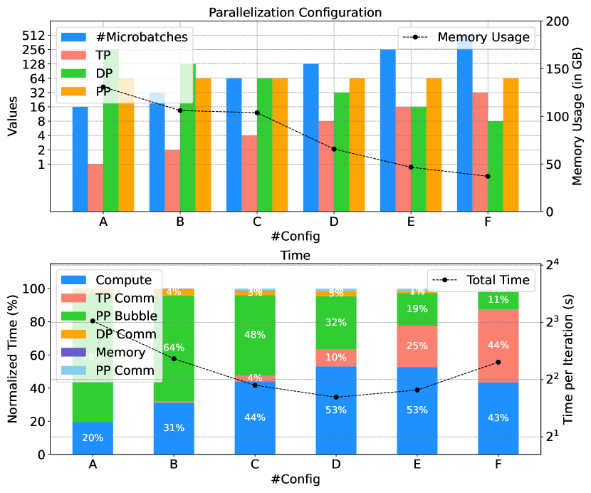
Figure 1: On $16384$ B200 with NVS domain size $n_{\text{{NVS}}}=8$, microbatch size $1$ for GPT3-1T with 1D TP: (top) Configurations (Config.) chosen with PP fixed to $n_{p}=64$ and the others varying. Example, Config. D is $(m,n_{t},n_{d},n_{p})=(128,8,32,64)$ and so on. (bottom) Time for each configuration broken down by the time spent on compute, memory accesses, various communications (DP, TP, PP) and PP bubbles. In config. D (TP $n_{t}=8$), we observe a local minimum in time per iteration.

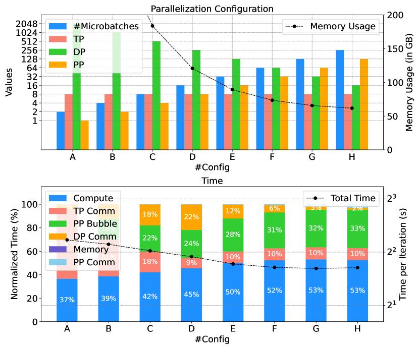
(a) $n_{\text{NVS}}=8$

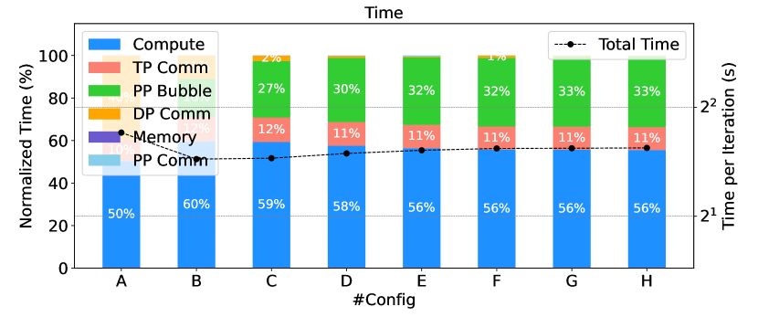
(b) $n_{\text{NVS}}=64$

Figure 2: Following Fig, 1, we change the following: we fix TP $n_{t}=8$ and vary PP and DP on two different NVS domain sizes. (top) We observe a local minimum at PP $n_{p}=64$. (bottom) For larger NVS, we observe that the local minimum shifts to low PP $n_{p}=2$, with NVS used to hide DP costs.

(Q1) Rationale behind optimal configurations. It is challenging to visualize the entire design space to understand the rationale behind an optimal configuration. We make it easier to reason about design choices by fixing certain configurations and varying others. In subsequent analysis ((Q2), (Q3)), we identify the optimal configuration by running the search (S3) over the entire design space.

For this analysis, we start with fixed total GPUs $n$ and global batch size $b$. Then, we vary any two parallelization parameters and keep the rest fixed. Since $n=n_{1}\times n_{2}\times n_{d}\times n_{p}$, as one configuration parameter increases, the other must decrease. Once we have chosen our parallelization configuration, we search over all possible GPU assignment configurations for each parallelization configuration to get the optimal assignment to the NVS domain. This ensures that, for any parallelization configuration, the assignment to NVS domain is optimal. We use the GPT3-1T transformer for this analysis. We make several observations.

(i) A simple observation is the apparent convex behavior of training time in the design space, especially w.r.t TP (tensor parallelism). In Fig. 1, assuming a fixed system (B200 and $n_{\text{{NVS}}}=8$) and 1D TP, we fix PP $n_{p}=64$ and vary both TP and DP (with the total GPUs fixed at $n=16384$ and microbatch size 1), to get training time as a function of varying TP/DP. We can immediately see the convexity of time that arises due to dominant costs from increased TP and DP. Note that as DP decreases, since global batch size $b$ and microbatch size $b_{m}$ are fixed, the number of microbatches ($m$) automatically increases. We see that greater TP drops the HBM usage but exhibits high communication costs (due to more microbatches). With large DP, number of microbatches reduces leading to large pipeline bubbles. The DP and PP communications are sufficiently small and hidden here. Hence, there is a local minimum around $n_{t}=8,n_{d}=32,m=128$ with about 40G HBM utilization.

(ii) The dual-bandwidth domain introduces subtle non-convexities in the training time within the design space. We show this by fixing TP at $n_{t}=8$ (for 1D TP), and varying PP and DP in Fig. 2. As DP increases, the DP communications follow a non-convex pattern, increasing to a peak transition point and then declining. This is due to the dual bandwidth domain where the chosen $n_{\text{{NVS}d}}$ (number of DP GPUs on NVS) starts to increase at the transition point—both TP and DP begin to utilize the fast bandwidth, decreasing the DP communication time. With maximum DP, all 8 NVS GPUs are utilized for DP. The local minimum is still the same.

(iii) Larger NVS domains can exploit the above by favoring alternate parallelization strategies. To show this, we repeat the the above experiment for $n_{\text{{NVS}}}=64$ in Fig. 2(b). We observe that the optimal configuration shifts to heavily decreased PP with the entire NVS domain used for DP and TP. Hence, the larger NVS domain has favored increased data parallelism with minimal pipelining, at the cost of increased HBM utilization. Note that while $n_{p}=1$ is fastest, it is infeasible on a B200 GPU due to high HBM capacity required.

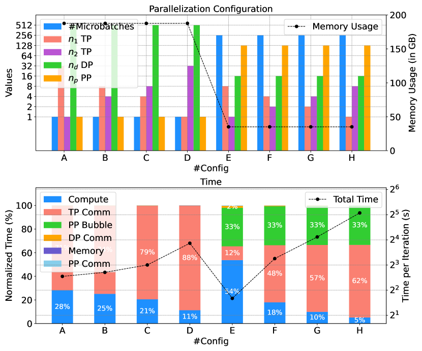
(a) $n_{\text{NVS}}=8$

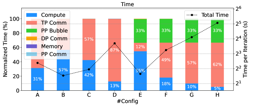
(b) $n_{\text{NVS}}=64$

Figure 3: For GPT3-1T with 2D TP SUMMA, we fix TP $(n_{t},n_{p})=(32,1)$ and vary $n_{1},n_{2}$ to get the the first five configurations and then switch to $(n_{t},n_{p})=(8,128)$ and repeat the same for the rest. We show two NVS domain sizes. With larger NVS, large DP (low PP) is preferred.

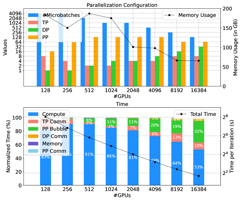
(a) GPT3-1T with 1D TP

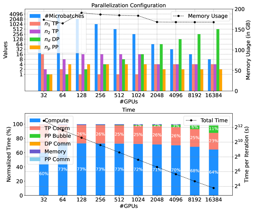
(b) ViT with 2D TP

Figure 4: On B200 with $n_{\text{{NVS}}}=8$: (top) Optimal parallelization strategy and HBM memory consumed vs number of GPUs (bottom) Time vs number of GPUs broken down by the time. For both models, most time is spent in compute. For GPT3-1T (left), 1D TP is sufficient to get good performance. PP bubbles start to dominate at scale, followed by TP and DP communication. HBM memory used also drops at scale. For ViT (right), 2D-TP is necessary for fitting the model on HBM and most of it is utilized, even at scale. TP communications are the main bottleneck followed by PP bubbles.

(iv) Higher dimensional 2D TP versions can show similar behaviors with the design-space being more complex due to additional TP dimensions. We sweep over two sets of configurations in Fig. 3 to show this in 2D TP SUMMA. We focus on the two extremes we observed in the 1D case (high PP and high DP). We first set high DP by fixing $n_{p}=1$, one microbatch $m=1$, and choosing a large enough TP $n_{t}=32$. We note that the microbatch size is now 8 and the memory efficiency of 2D TP SUMMA enables us to fit the model on HBM; 1D TP would need far greater TP for this microbatch size and $n_{p}=1$ due to shared activation memory, leading to unmanageable communication costs. We then only vary the relative TP allocation into $n_{1}$ and $n_{2}$. Next, we switch to low DP by setting $n_{p}=128$ and repeat with $n_{t}=8$. We retain large $m$ here to manage the pipeline bubbles (since $n_{p}>1$). We observe that in both high and low DP configurations the fastest configuration involves only 1D TP with $n_{2}=1$. This is because adding the second dimension increases the communication volume significantly in SUMMA (as noted in §III) and, while more GPUs can decrease this (since SUMMA communication volumes scale with number of GPUs), the slow IB bandwidth creates bottlenecks. In Fig. 3(a), $(n_{1},n_{2},n_{p})=(8,1,128)$ is fastest. Increasing the NVS domain size to $64$, in Fig. 3(b), favors high DP (similar to 1D TP) with $(n_{1},n_{2},n_{p})=(8,4,1)$ being fastest. The fast bandwidth helps manage and balance the large TP costs from both dimensions with effectively no PP. Note that, here, the DP communications are effectively hidden behind the increased compute of a large microbatch size. 2D TP is also similar but shows higher memory pressure from shared weights and activations (see Fig. 2 for details).

(Q2) Optimal parallelization strategy as a function of transformer type. We show the optimal parallelization strategy from the performance model as a function of number of GPUs $n$ in Fig. 4 on B200 with $n_{\text{{NVS}}}=8$. To get the optimal configuration (note that this includes the parallelization configurations as well as assignment of GPUs to NVS domains), we run our search (S3) for each $n$, independently. In these plots, we also note the difference that the $x$ axis now enumerates an increasing number of GPUs on which the models are parallelized, and for each scale ($n$) we show the optimal configuration and time breakdown in the same format as previous figures. These plots show the strong scaling behavior of the transformer and highlights how parallelization configurations and training time bottlenecks change with the use of more GPUs for training. We make the following observations.

(i) The optimal parallelization configurations for GPT3-1T are re-balanced as $n$ changes due to different bottlenecks arising at different scales. We show this in Fig. 4(a) assuming a B200 system with $n_{\text{{NVS}}}=8$. At small GPU scales (128, 256), the performance model opted to use increased TP to fit the model, leading to large TP communication. At larger scales, TP reduces and then increases monotonically. PP increases to the maximum value (depth $d$) until 4096 GPUs. At this point, DP has increased to the point that the number of microbatches (which reduce with more DP) are not large enough to hide the pipeline bubbles, seen in the increasing pipeline bubble fractions, and PP starts to reduce. Smaller PP exposes more TP communication and hence the optimal configuration carefully re-balances each of these at different scales to manage the bottlenecks. Finally, DP and TP communications are insignificant at small scale, but at large scale they slowly get exposed.

(ii) Each GPU scale shows a different optimal assignment of GPUs onto the NVS domain for GPT3-1T. For example, at 2048 GPUs, the performance model opted $(n_{\text{{NVS}1}},n_{\text{{NVS}p}})=(4,2)$ (note that NVS size is $n_{\text{{NVS}}}=8)$, at 1024 GPUs we see $(n_{\text{{NVS}1}},n_{\text{{NVS}d}},n_{\text{{NVS}p}})=(2,2,2)$ and the full NVS domain is used for TP at 8192 GPUs and beyond. Hence, the fast bandwidth is exploited differently across various $n$ for each parallelization strategy, to better hide their respective dominating costs.

(iii) HBM capacity utilization is high only at small-to-moderate GPU scales and drops at larger scale for GPT3-1T. We also note that memory access time is insignificant at all scales for this transformer with compute being the dominant cost, followed by pipeline bubbles, TP communication and small DP/PP communications at large scale. 2D TP versions show similar behavior with re-balanced configurations, HBM utilization, and dominant bottlenecks at different scales (see Fig. 3 as an example).

(iv) In ViT, sequence length $l=64\text{K}$ renders 1D TP infeasible on all GPUs due to extremely large activation map memory, with 2D TP necessary and dominating the optimal configurations. We show the ViT 2D TP in Fig. 4(b). Due to large $l$, large TP is necessary with $n_{1}=4$ and $n_{2}=4$ as the most common strategy at scale. PP is low and TP communications are the only bottlenecks. While PP helps reduce weights memory, it increases activation memory as noted in §III as the 1F1B schedule stores $n_{p}$ microbatches of activation maps. Only TP helps in this model setting at the cost of high communication time—the full NVS domain is used only for TP. HBM capacity is also highly utilized. 2D TP SUMMA exhibits similar behaviors with a smaller throughput (due to increased communication) but is more memory efficient.

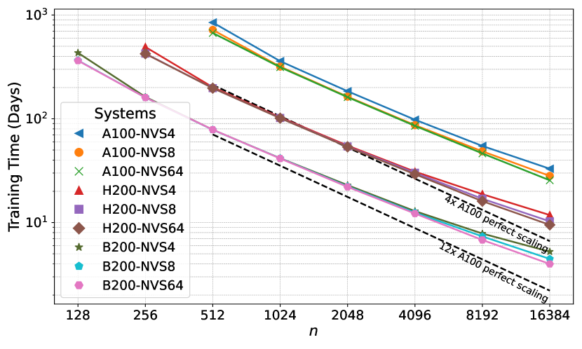
(a) GPT3-1T with 1D TP

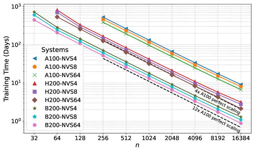
(b) ViT with 2D TP

Figure 5: Training time in days vs number of GPUs ($n$) for different GPUs (A100, H200, B200). We also assume different NVS domain sizes for each generation—NVS4 indicates $n_{\text{{NVS}}}=4$ and so on (top) Training time on 1T tokens for GPT3-1T using 1D TP. We see a consistent improvement across GPU generations. Further, smaller number of future GPUs are capable of training GPT3-1T due to larger HBM. NVS effects are seen at the smallest scale (due to increased TP) and at the largest scales. (bottom) Training time on 40 years of ERA5 with a ViT using 2D TP. While GPU generations provide similar advantages, NVS domain size effects are seen throughout due to increased TP necessary for this model.

(Q3) Overall Performance, GPU Generation, and NVS Domain Size. We show the training time vs number of GPUs for the two models for different GPU generations (A100, H200, B200) as well as different NVS domain sizes (4, 8, and 64) in Fig. 5. We make the following observations:

(i) The GPT3-1T model benefits significantly with higher GPU generation. We show this in Fig. 5(a), where the training times are $\mathcal{O}$(30) days on $16K$ A100 GPUs and it drastically drops to $\mathcal{O}$(3-5) days on the B200 GPU, owing to increased tensor core performance and network bandwidths. We also show this in Figs. 5 and 6 where we sweep over different hardware characteristics and highlight the reduced sensitivity to capacity/HBM bandwidth and also show that configurations with small memory bandwidth and high capacity can also show good performance, highlighting the value of alternate memory technologies. Pre-training this model would require $>10K$ GPUs to keep training reasonable at $\mathcal{O}$(days), even for the B200, emphasizing the importance of understanding performance bottlenecks at scale.

(ii) The NVS domain effects are only seen at large scale (and increasing with scale) for the GPT3-1T model, where the larger domains increase the scalability of the model. As noted in Q1, this is because larger NVS domain allows large DP (at the cost of higher memory usage) by hiding the DP communication costs which, in turn, decreases pipeline bubbles (that dominate the bottlenecks at scale) thereby improving scalability. Hence, with large NVS as well, TP remains small with the NVS domain utilized for DP to scale better (see Fig. 3). At the small scale, the NVS domain again plays a role due to heavy parallelism to fit the model on available GPUs. At moderate scale, the effects are milder—fine-tuning jobs at this scale may not see a lot of benefit from larger NVS domains. Similarly, the NVS domain helps more for the A100 GPUs due to its limited capacity, leading to increased TP.

(iii) While 1D TP is performant for GPT3-1T, both 2D TP versions can help further reduce training time (see Fig. 4 for relative speedups). We observe that 2D TP SUMMA can particularly help in the resource constrained regime—smaller number of GPUs, small capacity (as in A100), and small NVS domain size. The speedups reduce as the GPU generation increases. Similar to 1D, as the NVS domain becomes larger, the 2D TP versions can also utilize it in favor of increased DP (see Fig. 3), increasing the scalability of the model.

(iv) The ViT also sees significant improvements with GPU generation. However, the 2D versions of TP are the only viable strategies, with 2D TP being optimal. Both HBM capacity as well as NVS domain size effects show more uniform importance across scales (also see Fig. 5(b)). This is due to the increased pressure placed on TP to fit long sequences. For this model, since $n_{t}=16$ is necessary any NVS domain size less than this will show performance drops. Hence, larger NVS domains add consistent value until $n_{t}$ GPUs are within the same domain, after which there are diminishing returns. We show that the ViT also shows alternate large capacity/low memory bandwidth configurations (alternate memory to HBM) as viable options in Fig. 6(b).

Empirical Validation. We verify that the performance model produces reasonable outputs for the different model types and parallelization strategies at scale. We consider moderate scale tests on 512 GPUs with global batch size 1024 on the Perlmutter [47] supercomputer at NERSC. Perlmutter has 4 A100 GPUs per node (all-to-all connected via NVLink). We validate the performance model with a 175B parameter GPT3 and a 32K ViT model using Megatron-LM [38]. We validate the optimal configuration from the performance model as well as few sub-optimal configurations. For GPT3, we observe that the optimal configuration $(n_{t},n_{p},n_{d},b_{m})=(4,16,8,1)$ shows a 11% error in iteration time. We test 4 other sub-optimal configurations (with different relative TP/PP/DP) and they show 4–15% errors. For the ViT, a near-optimal configuration $(n_{1},n_{2},n_{p},n_{d},b_{m})=(2,4,4,16,1)$ (the optimal configuration overflowed HBM due to extra scaffolding memory in PyTorch; we picked the next configuration), the error is about 2%. For sub-optimal configurations, with different TP/PP/DP, the error ranges from 11–26%. We observe performance trends between observed and predicted iteration times are consistent (larger observed times seen with larger predicted times) and the low errors are encouraging.

V Summary and Discussion

We have described the core components of an analytical performance model and its sensitivity to the transformer architecture, system features, and parallelization strategy. We observe the following high-level characteristics: (i) Placement of GPU groups within NVS domain can significantly affect the performance, motivating software codebases to be flexible in not just the parallel configuration, but also the GPUs used for the configuration; (ii) GPT3-1T class models can benefit greatly with larger NVS domains in pre-training scales ($>10K$ GPUs), where $\mathcal{O}$(days) improvements can be significant; (iii) Smaller (and moderate) scales of fine-tuning demand more from HBM and less from NVS ($\mathcal{O}$(hours) improvements), suggesting different system design choices based on the training regime of large models. SUMMA variants of TP can particularly help at small scales and in resource-constrained regimes (small capacity, small NVS); (iv) ViT class models demonstrate a contrasting extreme with more dependence on NVS, HBM, and higher-dimensional parallelism (with 2D TP variants). SUMMA variants can reduce some memory pressure, but heavy dependence on expensive system features may motivate algorithmic advances for reduced sequence length training; (v) Both models benefit most from FP16 tensor core performance and network bandwidths, but other memory technologies (lower bandwidths/more capacity like LPDDR) can be viable alternatives which may help alleviate the heavy dependence on the NVS for ViT class models.

Limitations. While several components are modeled in the performance model, there are some optimizations we do not consider. We do not consider interleaved pipeline schedules [16] that can drop bubble time further. There are more lower-level opportunities for TP communications to be overlapped with compute to drop communication time. Weights (and gradients) can also be partitioned using DP at the cost of higher communication introducing another trade-off. We also do not explore offloading to the CPU (in addition to HBM) which may be very useful for large sequences.

Outlook. Overall, this work emphasizes the need to closely explore the complex interplay between architecture type beyond LLMs, parallelization strategies beyond 3D to 4D (and higher) versions, and the HPC system (interconnects and accelerator features), and demonstrates a path towards a tightly coupled modeling of all these elements. We focus our future work in including more optimizations, detailed analyses of 2D TP versions, and other architecture types such as linear (or windowed) attention versions of the ViT, spectral transformer models, convolutional models, graph neural networks, amongst other scientific AI foundation models.

-A Methods: Additional Details

We outline the abbreviations used in this paper in Tab. A1.

Abbreviation	Description
NVS	NVSwitch
IB	InfiniBand
HBM	High-bandwidth memory
S/A	Self-attention layer
MLP	Multi-layer Perceptron layer
LN	LayerNorm layer
L/A	Logit-Attend layer
SM	Softmax layer
DP	Data parallelism
TP	Tensor parallelism
2D TP	2D tensor parallelism
2D TP SUMMA	2D tensor parallelism with SUMMA matrix-multiply
PP	Pipeline parallelism

TABLE A1: Abbreviations used in this paper.

We now outline some additional details regarding the performance model.

(S1) Backward pass. Assuming the matrix multiply, $\mathbf{C}=\mathbf{A}\mathbf{B}$ where $\mathbf{C}\in\mathbb{R}^{m\times n},\mathbf{A}\in\mathbb{R}^{m\times k},\mathbf{B}\in\mathbb{R}^{k\times n}$, the backward pass computes the gradient tensors of the loss function $\mathcal{L}$:

$$\frac{\partial\mathcal{L}}{\partial\mathbf{A}} =\frac{\partial\mathcal{L}}{\partial\mathbf{C}}\mathbf{B}^{T},\frac{\partial\mathcal{L}}{\partial\mathbf{B}}=\mathbf{A}^{T}\frac{\partial\mathcal{L}}{\partial\mathbf{C}}$$

Note that $\mathbf{A},\mathbf{B}$ are intermediate maps stored for the backward pass in HBM. $\mathbf{B}$ may be weights (in MLPs) or activation maps (in L/A). Similar FLOPs, bytes and communication volumes can be derived for the backward pass (typically incurring twice the cost of the forward pass).

(S1) 2D TP SUMMA. Scalable Universal Matrix Multiplication (SUMMA) [28] is an efficient distributed matrix multiply algorithm that uses a 2D grid of processors (GPUs) $n_{1}\times n_{2}$.

Algorithm 1 $\mathbf{C}=\mathbf{A}\mathbf{B}$ using SUMMA

1:Input: $\mathbf{A}_{ij}$, $\mathbf{B}_{ij}$

2:Output: $\mathbf{C}_{ij}$

3:$\mathbf{C}=0$

4:for $\kappa=0\to n_{b}-1$ do

5:     for $i=0,...,n_{1}-1$ Broadcast $\mathbf{A}^{\kappa}_{i}$ to $i^{th}$ process row

6:     for $j=0,...,n_{2}-1$ Broadcast $\mathbf{B}^{\kappa}_{j}$ to $j^{th}$ process col

7:     $\mathbf{C}_{ij}=\mathbf{C}_{ij}+\mathbf{A}^{\kappa}_{i}\mathbf{B}^{\kappa}_{j}$

8:end for

9:return $\mathbf{C}_{ij}$

While many implementations of SUMMA [34] assume square matrices and process grids, SUMMA does not impose these restrictions and we outline the general algorithm here. Each matrix is evenly partitioned into $n_{1}\times n_{2}$ sub-blocks and mapped onto their respective GPUs. In the rectangular version of SUMMA [48], we assume that $k$ is further divided into $n_{b}$ “panels”, each of size $k_{b}$. Denoting the panels as $\mathbf{A}^{\kappa}=\mathbf{A}_{0:m-1,k^{\prime}:k^{\prime\prime}},\mathbf{B}^{\kappa}=\mathbf{B}_{k^{\prime}:k^{\prime\prime},0:n-1}$ with $k^{\prime}=\kappa k_{b}$ and $k^{\prime\prime}=(\kappa+1)k_{b}-1$, SUMMA recasts the matrix multiply as:

$$\mathbf{C}=\sum_{\kappa}^{n_{b}-1}\mathbf{A}^{\kappa}\mathbf{B}^{\kappa}.$$

Assuming the matrices are distributed as $\mathbf{A}_{ij},\mathbf{B}_{ij},\mathbf{C}_{ij}$, with $i=0,1,...,n_{1}-1,j=0,1,...,n_{2}-1$, and $\mathbf{A}^{\kappa}_{i}$ denotes panel at the $i^{th}$ row and $\mathbf{B}^{\kappa}_{j}$ denotes panel at the $j^{th}$ column, we show the SUMMA pseudo-code in Algorithm 1. The pseudo-code of $\mathbf{C}=\mathbf{A}^{T}\mathbf{B}$ and $\mathbf{C}=\mathbf{A}\mathbf{B}^{T}$ are similar but have a Broadcast and Reduce collective, instead of two Broadcasts (see [28] for more details).

Operation	Partitioned Tensor Shapes	Type	Vol
2D TP with SUMMA over $n_{1}\times n_{2}$ grid of GPUs
SA
$\tilde{\mathbf{X}}=\text{LN}(\mathbf{X})$	$\tilde{\mathbf{X}}:(b,\frac{l}{n_{2}},\frac{e}{n_{1}})$, $\mathbf{X}:(b,\frac{l}{n_{2}},\frac{e}{n_{1}})$,	$\mathcal{AR}$	$b\frac{l}{n_{2}}e$
$\mathbf{Q}=\tilde{\mathbf{X}}\mathbf{W_{Q}}$	$\mathbf{Q}:(b,\frac{h}{n_{1}},\frac{l}{n_{2}},e_{h})$, $\mathbf{W_{Q}}:(\frac{e}{n_{2}},\frac{e}{n_{1}})$,	$\mathcal{B}$	$V_{1}$
$\mathbf{A}=\mathbf{Q}\mathbf{K}^{T}$	$\mathbf{A}:(b,\frac{h}{n_{1}},\frac{l}{n_{2}},l)$, $\mathbf{K}:(b,\frac{h}{n_{1}},l,e_{h})$	$\mathcal{AG}$	$bl\frac{e}{n_{1}}$
$\mathbf{S}=\mathbf{A}\mathbf{V}$	$\mathbf{S}:(b,\frac{h}{n_{1}},\frac{l}{n_{2}},e_{h})$, $\mathbf{V}:(b,\frac{h}{n_{1}},l,e_{h})$	$\mathcal{AG}$	$bl\frac{e}{n_{1}}$
$\mathbf{Y}=\mathbf{S}\mathbf{W_{p}}$	$\mathbf{Y}:(b,\frac{l}{n_{1}n_{2}},e)$, $\mathbf{W_{p}}:(\frac{e}{n_{1}},e)$	$\mathcal{RS}$	$b\frac{l}{n_{2}}e$
MLP
$\tilde{\mathbf{Y}}=\text{LN}(\mathbf{Y})$	$\tilde{\mathbf{Y}}:(b,\frac{l}{n_{2}},\frac{e}{n_{1}})$, $\mathbf{Y}:(b,\frac{l}{n_{2}},\frac{e}{n_{1}})$,	$\mathcal{AR}$	$b\frac{l}{n_{2}}e$
$\mathbf{Z}=\tilde{\mathbf{Y}}\mathbf{W_{1}}$	$\mathbf{Z}:(b,\frac{l}{n_{2}},\frac{f}{n_{1}})$, $\mathbf{W_{1}}:(\frac{e}{n_{2}},\frac{f}{n_{1}})$	$\mathcal{B}$	$V_{2}$
$\mathbf{X}=\mathbf{Z}\mathbf{W_{2}}$	$\mathbf{X}:(b,\frac{l}{n_{2}},\frac{e}{n_{1}})$, $\mathbf{W_{2}}:(\frac{f}{n_{2}},\frac{e}{n_{1}})$	$\mathcal{B}$	$V_{3}$

TABLE A2: 2D TP SUMMA: Tensor shapes, communication collective and volume (vol: total bytes transferred per GPU) for different operations. $\mathcal{AG}$ is AllGather, $\mathcal{RS}$ is ReduceScatter, $\mathcal{B}$ is Broadcast, and $\mathcal{AR}$ is AllReduce. $\mathbf{K},\mathbf{V}$ follow $\mathbf{Q}$. Communication volume scales with one GPU dimension and there are no shared weights. For the SUMMA multiplies, $V_{1}=ble/n_{2}+e^{2}/n_{1},V_{2}=V_{3}=ble/n_{2}+ef/n_{1}$.

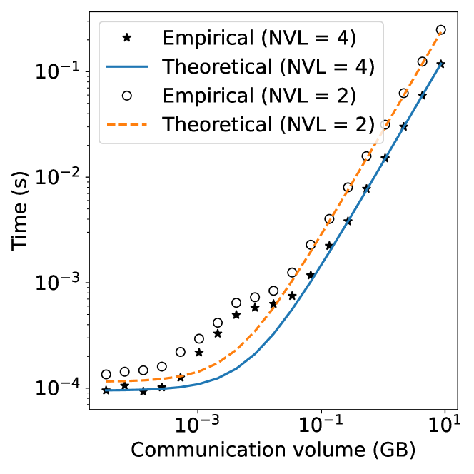
Figure 1: Time for $\mathcal{AG}$ as a function of communication volume on 32 A100 GPUs. We compare empirical numbers on Perlmutter through NCCL tests [41] to our theoretical formulae for different fast domain (NVLink) sizes. For NVL 2, 2 GPUs per node are used and for NVL 4, 4 GPUs per node are used. We see that more GPUs per node effectively increases the SlingShot bandwidth, leading to smaller times.

(S2) Communication in TP. We show the full SUMMA communicaton and tensor shapes in Tab. A2. Note that $V_{1},V_{2},V_{3}$ all communicate the weights as well as the activation maps, increasing the absolute volume but showing better scaling with $n_{1},n_{2}$. For the forward pass, in 1D TP, the communications outlined in Tab. I are assumed to be non-overlapped since partial sums are assumed to be computed before the communication can take place and the subsequent layers need to wait for the synced activation map. 2D TP is similar with the $l$ partitions being embarrassingly parallel. In SUMMA, we assume some overlap of the TP communications. There is a prologue time $t_{\text{prologue}}$ to perform two broadcasts before the first $\kappa$ iteration and the rest of the broadcasts (for subsequent $\kappa$ iterations) can be scheduled asynchronously (and hence overlapped) to the computation of $\mathbf{C}_{ij}$. Hence, the communication time $t_{\text{comm}}=t_{\text{prologue}}+n_{b}t_{\text{exposed}}$, with $t_{\text{exposed}}$ as the exposed time between two broadcasts and the compute. Hence, the $n_{b}$ parameter can influence $t_{\text{comm}}$ as larger values will reduce $t_{\text{prologue}}$ (smaller panels communicated) but at the same time reduce the matrix multiply efficiency (smaller matrices, may become memory bound with small inner dimensions), exposing communication more. Hence, the 2D TP configuration also searches over $n_{b}$. In the backward pass, 1D TP incurs similar $\mathcal{AG}$ and $\mathcal{RS}$ in a conjugate fashion to the forward pass communications due to the transposed matrix multiplies. In 2D TP, the weight gradients incur an additional reduction across $n_{2}$ due to the partitioned $l$ dimension. We assume this TP communication to be overlapped and scheduled with the DP communications—the weight gradient $\mathcal{RS}$ and the weights $\mathcal{AG}$ happen across the combined $n_{d}\times n_{2}$ GPU group. For SUMMA, the transposed matrix multiples incur a Broadcast and Reduce instead of two Broadcasts.

Description	A100	H200	B200
Tensor core FP16 (TFLOPs/s)	312	990	2500
Vector FP16 (TFLOPs/s)	78	134	339
Flops Latency (s)	2e-5	2e-5	2e-5
HBM Bandwidth (GB/s)	1555	4800	8000
HBM Capacity (GB)	80	141	192
NVS 1-directional Bandwidth (GB/s)	300	450	900
NVS Latency (s)	2.5e-6	2.5e-6	2.5e-6
IB Bandwidth (GB/s)	25	50	100
IB Latency (s)	5e-6	5e-6	5e-6

TABLE A3: GPU and network parameters for various GPU generations.

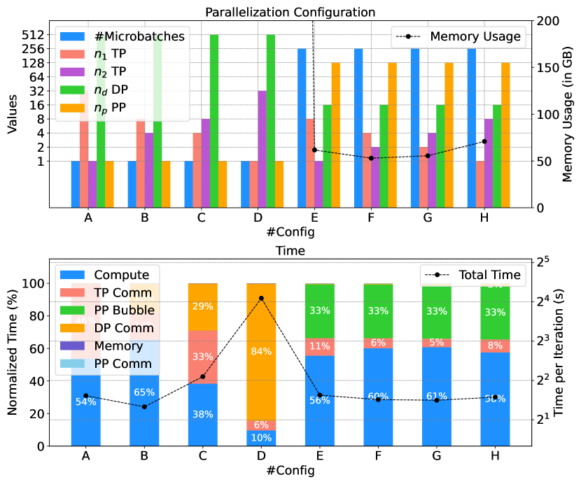
(a) GPT3-1T with 2D TP

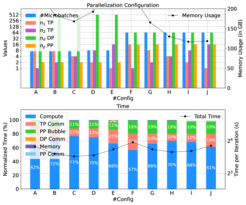
(b) ViT with 2D TP

Figure 2: (a) For GPT3-1T with 2D TP, we fix TP $n_{t}=32,n_{p}=1$ and vary $n_{1},n_{2}$ to get the the first five configurations and then switch to $n_{p}=128$ and repeat the same with $n_{t}=8$ for the last four configurations. We use a B200 GPU with NVS domain size $n_{\text{{NVS}}}=64$, global batch size $4096$ on $16384$ GPUs and also show time for each configuration broken down by the components. We see similar behavior as 2D TP SUMMA but the memory consumed is very high and hence the large PP configurations are chosen. (b) For ViT with 2D TP, we first fix $n_{t}=16$ and vary $n_{1},n_{2}$, then switch to $n_{p}=16$ and repeat the same. The memory used is sensitive to the parallelization regime.

(S2) Validating communication time of collectives. We validate our time to communication formulae for the different communication collectives on the Perlmutter [47] supercomputer at NERSC. Perlmutter has 4 A100 GPUs per node connected via 4 third generation NVLinks between each pair of GPUs (with all GPUs interconnected) and 4 NICs per node for the SlingShot communications (similar to IB). While there is no NVSwitch on Perlmutter, we can derive equivalent expressions for NVLink based on number of NVLinks per GPU used in the collective. For example, if only 2 GPUs per node were used, only 4 NVLinks are used for the fast bandwidth. If all 4 GPUs are used in a node, then 12 NVLinks are used. In Fig. 1, we show that our theoretical time formulae agree well with the empirical results. We also see the effect of the increased SlingShot bandwidth if more GPUs are used per node (in the fast domain). We observe some non-linear latency effects at small volumes and do not model these in our performance model. We also verify the above agreement over a range of GPUs (and nodes), and also for other collectives.

(S2) Hardware configurations. We summarize the hardware parameters used in our model. The specifications for the A100 GPU can be found in [49], and the H200 and B200 GPUS can be found respectively in  [50] and [51]. Each GPU generation is coupled to its respective NVLink generation. Similarly, the IB interconnects improve with each generation, from ConnectX-6 [52], to ConnectX-7 [53], and the most recent ConnectX-8 [54]. We assume network latency values from the previous validation experiments and also assume they do not greatly improve with newer generations. In our experiments on Perlmutter, we observe typical bandwidth efficiencies of 70% for the networks and include this as an efficiency parameter as well. For FLOPs, we assume a simple model based on [55]: $t_{\text{flops}}=t_{\text{sf}}+\lambda_{f}/\lambda_{fh}$, where the FLOPs latency $t_{\text{sf}}$ can be inferred from [55] and models the inefficiency in matrix multiplies of small matrices to the first order.

Software environment setup for validation. We validate our performance model in IV with the open source Megatron-LM codebase [38]. We use NVIDIA PyTorch NGC container v24.05 and build Megatron-LM in the container. The GPT3-175B and custom ViT models are built on top of TransformerEngine and FlashAttention-2. For optimized collective operations, NCCL v2.19.4 and its associated plugin for Perlmutter is used. Iteration times are captured using the built-in logging utility in Megatron-LM. We use the CodeParrot [56] dataset for empirical validation experiments. This dataset is pre-processed by existing tools provided in Megatron-LM. The following optimizations are enabled during training: distributed optimizer, overlapping gradient reduction, overlapping parameter all-gather in the distributed optimizer, half precision (FP16) along with Flash Attention. To test different strategies that require mapping different ranks on different devices on and across nodes, we tweak the model parallel initialization to accept different mapping orders in the form of strings, for example, tp-cp-dp-pp, cp-tp-pp-dp, etc.

-B Additional Results

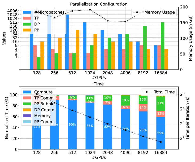
(a) GPT3-1T 1D TP on $n_{\text{{NVS}}}=64$

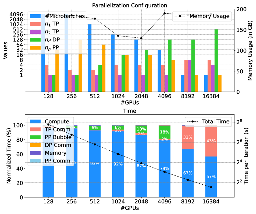
(b) GPT3-1T 2D TP SUMMA on $n_{\text{{NVS}}}=64$

Figure 3: On B200 GPU with global batch size $4096$: (top) Optimal parallelization strategy and HBM memory consumed vs number of GPUs (bottom) Time vs number of GPUs broken down by different components. (a) GPT3-1T with 1D TP on larger NVS domain shows reduced PP at scale (b) GPT3-1T with 2D TP SUMMA shows mostly 1D TP except at scale due to the large NVS domain.

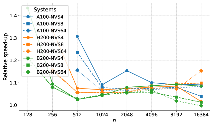
(a) Speedup for 2D TP SUMMA w.r.t 1D TP

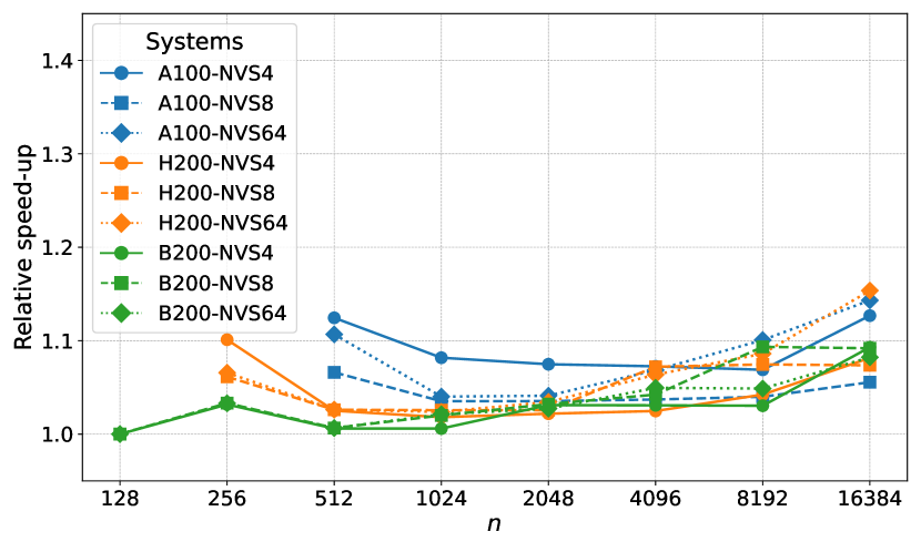
(b) Speedup for 2D TP w.r.t 1D TP

Figure 4: We show the relative speedup in training time of the two 2D TP strategies with respect to 1D TP. The speedups are colored according to GPU generations and marked according to NVS domain size. We observe that both versions provide good speedups of about 10% with SUMMA particularly helpful at resource constrained regimes (small scale, capacity, NVS domain size). 2D TP is more performant at the large scales. Higher GPU generations and NVS sizes decrease speedup in general.

2D TP rationale. In Fig. 2, we show that 2D TP works similarly to 2D TP SUMMA in GPT3-1T with low PP/high DP and low DP/high PP configurations as possible candidates. However, unlike 2D TP SUMMA, the low PP/high DP configurations take up a lot of memory since 2D TP has lot of shared weights and activation maps compared to SUMMA. Also, the DP communication times are shown to be high, but in 2D TP, this includes the weight gradients reduction across $n_{2}$ that is scheduled with the DP reductions—we do not disentangle this TP communication in our estimates. For the ViT, we show the 2D TP possibilies in Fig. 2(b). We still observe the high and low PP configurations contending with each other (with high TP necessary for this model), with the low PP configurations being favored here. We also see that the memory usage is sensitive to the choice of $n_{1}$, $n_{2}$ with $n_{p}$. For small PP, the weights memory dominates at low $n_{1}$ and activation memory dominates at low $n_{2}$. With high PP, the activation memory dominates and hence with more $n_{2}$, the memory comes down.

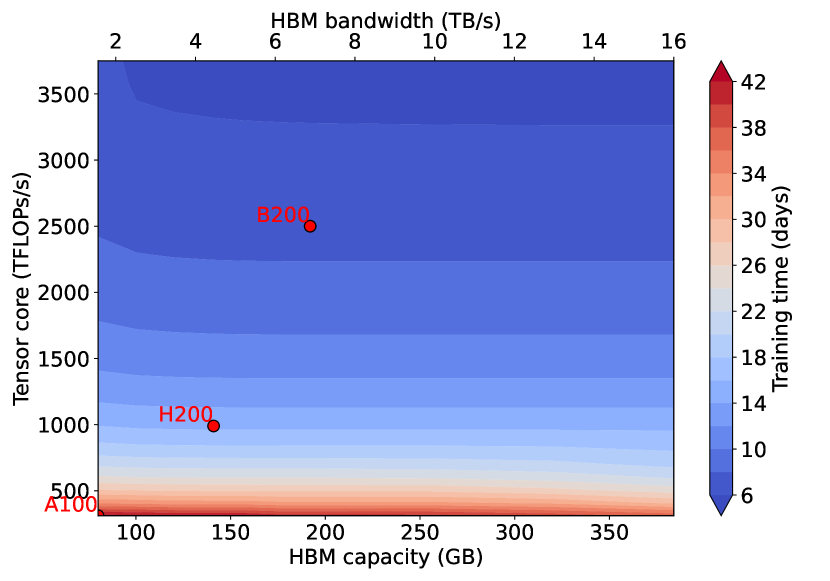
(a) GPT3-1T with 1D TP

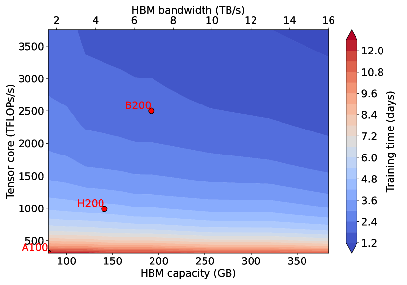
(b) ViT with 2D TP

Figure 5: Training times for GPT3-1T and ViT using 8192 GPUs as a function of FLOP rate (compute speed) and HBM memory capacity and bandwidth. NVS domain is 8 with fixed NVS and IB bandwidths at the B200 generation and the global batch size is $4096$. FLOP rates are the primary factor for speed-ups with bandwidth/capacity having different roles for the different models.

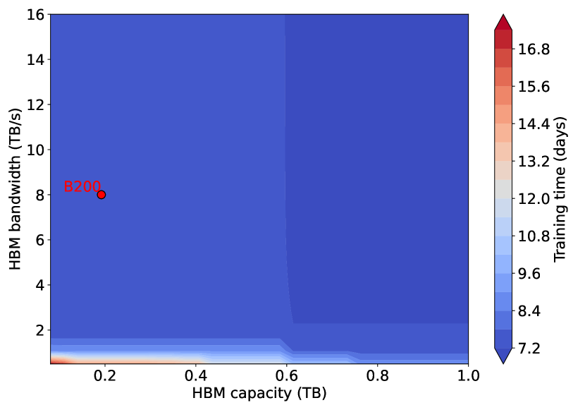
(a) GPT3-1T with 1D TP

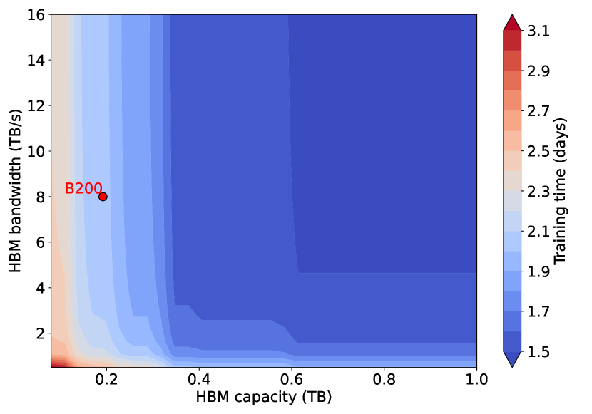
(b) ViT with 2D TP

Figure 6: Training time for GPT3-1T and ViT as function of HBM memory capacity and bandwidth. NVS domain is 8 with fixed NVS and IB bandwidths at the B200 generation (along with the FLOP rates) and the global batch size is $4096$. Both models show lower bandwidth/higher capacity configurations can contend in performance by trading-off lesser parallelism inefficiencies for higher memory access times.

Parallelization and model type. For GPT3-1T, we show 1D TP on a large NVS domain in Fig. 3(a). We see that small PP (and large DP) is favored at scale due to the large fast bandwidth domain. With 2D TP SUMMA, we see that, for GPT3-1T, the model effectively chooses 1D TP at most scales. Due to the large NVS domain, it chooses 2D partitioning at scale. For the ViT, the 2D TP SUMMA is very similar to 2D TP, with the latter showing better performance (training times) and the former showing better memory utilization.

Speedups with higher-dimensional TP. We show that both 2D TP versions for GPT3-1T can reduce training time. In Fig. 4, we show the speedup of the two 2D TP versions with respect to 1D TP for different GPU generations and NVS domain sizes. While the speedups are generally clustered for most systems, we observe speedups of approximately 5–10% across various GPU scales. 2D TP SUMMA is more helpful at very small scales, small capacities (A100), and smaller NVS. 2D TP shows similar speedups that are higher at the larger scale.

GPU memory bandwidth, capacity, and FLOP rate effects. In Fig. 5, we plot the training times for GPT3-1T and ViT as function of GPU compute vs HBM memory and bandwidth. To understand the impact of the GPU parameters alone, we maintain the same network architecture while scaling up the memory capacity and bandwidth on one axis, and the tensor core and vector FLOP rates on the other. We show both memory capacity and bandwidth on the x-axis and only the tensor core FLOPs/s on the y-axis without loss of generality. Also, we display in the plots three generations of GPUs (A100, H200, B200). As observed in §IV, GPT3-1T is less sensitive to HBM capacity and bandwidth at large scales, with tensor core FLOPs/s being the primary factor for performance boosts. For ViT, due to the large TP necessary for the long sequence model (see discussion in §IV around performance senstitivty to the model type), the capacity and bandwidth play a bigger role.

In Fig. 6, we use the B200 generation compute and network speeds and vary separately the HBM memory and bandwidth. We once again see the weak dependence on capacity and bandwidth for the GPT3-1T model—only very small bandwidths increase memory-bound operation times. However, we observe that large capacities and small bandwidths, representative of different memory technologies like LPDDR [57], show good performance, comparable to the B200. We see high-bandwidth/low-capacity configurations comparable to the low-bandwidth/high-capacity configurations, where lesser parallelism (and hence communication/bubbles) is traded off for larger memory access times. The ViT once again shows more sensitivity to the capacity and bandwidth with multiple inflection points, with smaller capacities showing poorer performance. However, again the high capacity, low bandwidth regions show good performance compared to the B200, highlighting alternate memory technologies may benefit training these models at certain scales. With more capacity, this can also help reduce the dependence of the ViT on NVS as lesser TP is required to fit the model.

References

- [1] https://github.com/ShashankSubramanian/transformer-perf-estimates, 2024.
- [2] A. Vaswani, N. Shazeer, N. Parmar, J. Uszkoreit, L. Jones, A. N. Gomez, L. u. Kaiser, and I. Polosukhin, “Attention is all you need,” in Advances in Neural Information Processing Systems, I. Guyon, U. V. Luxburg, S. Bengio, H. Wallach, R. Fergus, S. Vishwanathan, and R. Garnett, Eds., vol. 30. Curran Associates, Inc., 2017.
- [3] A. Radford, K. Narasimhan, T. Salimans, and I. Sutskever, “Improving language understanding with unsupervised learning,” 2018.
- [4] J. Devlin, M.-W. Chang, K. Lee, and K. Toutanova, “BERT: Pre-training of deep bidirectional transformers for language understanding,” in Proceedings of the 2019 Conference of the North American Chapter of the Association for Computational Linguistics: Human Language Technologies, Volume 1 (Long and Short Papers), J. Burstein, C. Doran, and T. Solorio, Eds. Minneapolis, Minnesota: Association for Computational Linguistics, Jun. 2019, pp. 4171–4186.
- [5] C. Raffel, N. Shazeer, A. Roberts, K. Lee, S. Narang, M. Matena, Y. Zhou, W. Li, and P. J. Liu, “Exploring the limits of transfer learning with a unified text-to-text transformer,” J. Mach. Learn. Res., vol. 21, no. 1, jan 2020.
- [6] L. Zhuang, L. Wayne, S. Ya, and Z. Jun, “A robustly optimized BERT pre-training approach with post-training,” in Proceedings of the 20th Chinese National Conference on Computational Linguistics, S. Li, M. Sun, Y. Liu, H. Wu, K. Liu, W. Che, S. He, and G. Rao, Eds. Huhhot, China: Chinese Information Processing Society of China, Aug. 2021, pp. 1218–1227.
- [7] Z. Du, Y. Qian, X. Liu, M. Ding, J. Qiu, Z. Yang, and J. Tang, “GLM: General language model pretraining with autoregressive blank infilling,” in Proceedings of the 60th Annual Meeting of the Association for Computational Linguistics (Volume 1: Long Papers), S. Muresan, P. Nakov, and A. Villavicencio, Eds. Dublin, Ireland: Association for Computational Linguistics, May 2022, pp. 320–335.
- [8] A. Kolesnikov, A. Dosovitskiy, D. Weissenborn, G. Heigold, J. Uszkoreit, L. Beyer, M. Minderer, M. Dehghani, N. Houlsby, S. Gelly, T. Unterthiner, and X. Zhai, “An image is worth 16x16 words: Transformers for image recognition at scale,” 2021.
- [9] A. El-Nouby, H. Touvron, M. Caron, P. Bojanowski, M. Douze, A. Joulin, I. Laptev, N. Neverova, G. Synnaeve, J. Verbeek, and H. Jégou, “Xcit: cross-covariance image transformers,” in Proceedings of the 35th International Conference on Neural Information Processing Systems, ser. NIPS ’21. Red Hook, NY, USA: Curran Associates Inc., 2021.
- [10] H. Touvron, M. Cord, M. Douze, F. Massa, A. Sablayrolles, and H. Jegou, “Training data-efficient image transformers & distillation through attention,” in Proceedings of the 38th International Conference on Machine Learning, ser. Proceedings of Machine Learning Research, M. Meila and T. Zhang, Eds., vol. 139. PMLR, 18–24 Jul 2021, pp. 10 347–10 357.
- [11] L. Chen, X. Zhong, F. Zhang, Y. Cheng, Y. Xu, Y. Qi, and H. Li, “Fuxi: A cascade machine learning forecasting system for 15-day global weather forecast,” npj Climate and Atmospheric Science, vol. 6, no. 1, p. 190, 2023.
- [12] C. Bodnar, W. P. Bruinsma, A. Lucic, M. Stanley, J. Brandstetter, P. Garvan, M. Riechert, J. Weyn, H. Dong, A. Vaughan et al., “Aurora: A foundation model of the atmosphere,” arXiv preprint arXiv:2405.13063, 2024.
- [13] T. Nguyen, J. Brandstetter, A. Kapoor, J. K. Gupta, and A. Grover, “Climax: A foundation model for weather and climate,” arXiv preprint arXiv:2301.10343, 2023.
- [14] J. Kaplan, S. McCandlish, T. Henighan, T. B. Brown, B. Chess, R. Child, S. Gray, A. Radford, J. Wu, and D. Amodei, “Scaling laws for neural language models,” arXiv preprint arXiv:2001.08361, 2020.
- [15] T. Brown, B. Mann, N. Ryder, M. Subbiah, J. D. Kaplan, P. Dhariwal, A. Neelakantan, P. Shyam, G. Sastry, A. Askell, S. Agarwal, A. Herbert-Voss, G. Krueger, T. Henighan, R. Child, A. Ramesh, D. Ziegler, J. Wu, C. Winter, C. Hesse, M. Chen, E. Sigler, M. Litwin, S. Gray, B. Chess, J. Clark, C. Berner, S. McCandlish, A. Radford, I. Sutskever, and D. Amodei, “Language models are few-shot learners,” in Advances in Neural Information Processing Systems, H. Larochelle, M. Ranzato, R. Hadsell, M. Balcan, and H. Lin, Eds., vol. 33. Curran Associates, Inc., 2020, pp. 1877–1901.
- [16] D. Narayanan, M. Shoeybi, J. Casper, P. LeGresley, M. Patwary, V. Korthikanti, D. Vainbrand, P. Kashinkunti, J. Bernauer, B. Catanzaro, A. Phanishayee, and M. Zaharia, “Efficient large-scale language model training on gpu clusters using megatron-lm,” in Proceedings of the International Conference for High Performance Computing, Networking, Storage and Analysis, ser. SC ’21. New York, NY, USA: Association for Computing Machinery, 2021.
- [17] S. Dash, I. R. Lyngaas, J. Yin, X. Wang, R. Egele, J. A. Ellis, M. Maiterth, G. Cong, F. Wang, and P. Balaprakash, “Optimizing distributed training on frontier for large language models,” in ISC High Performance 2024 Research Paper Proceedings (39th International Conference), 2024, pp. 1–11.
- [18] H. Sheng, X. Wu, X. Si, J. Li, S. Zhang, and X. Duan, “Seismic foundation model (sfm): a new generation deep learning model in geophysics,” arXiv preprint arXiv:2309.02791, 2023.
- [19] M. McCabe, B. R.-S. Blancard, L. H. Parker, R. Ohana, M. Cranmer, A. Bietti, M. Eickenberg, S. Golkar, G. Krawezik, F. Lanusse et al., “Multiple physics pretraining for physical surrogate models,” arXiv preprint arXiv:2310.02994, 2023.
- [20] J. Jumper, R. Evans, A. Pritzel, T. Green, M. Figurnov, O. Ronneberger, K. Tunyasuvunakool, R. Bates, A. Žídek, A. Potapenko et al., “Highly accurate protein structure prediction with alphafold,” nature, vol. 596, no. 7873, pp. 583–589, 2021.
- [21] Z. Lin, H. Akin, R. Rao, B. Hie, Z. Zhu, W. Lu, N. Smetanin, R. Verkuil, O. Kabeli, Y. Shmueli, A. dos Santos Costa, M. Fazel-Zarandi, T. Sercu, S. Candido, and A. Rives, “Evolutionary-scale prediction of atomic-level protein structure with a language model,” Science, vol. 379, no. 6637, pp. 1123–1130, 2023, earlier versions as preprint: bioRxiv 2022.07.20.500902. [Online]. Available: https://www.science.org/doi/abs/10.1126/science.ade2574
- [22] I. Batatia, P. Benner, Y. Chiang, A. M. Elena, D. P. Kovács, J. Riebesell, X. R. Advincula, M. Asta, W. J. Baldwin, N. Bernstein et al., “A foundation model for atomistic materials chemistry,” arXiv preprint arXiv:2401.00096, 2023.
- [23] M. Shoeybi, M. Patwary, R. Puri, P. LeGresley, J. Casper, and B. Catanzaro, “Megatron-lm: Training multi-billion parameter language models using model parallelism,” CoRR, vol. abs/1909.08053, 2019.
- [24] NVIDIA. (2024) Nvswitch and nvlink. [Online]. Available: https://www.nvidia.com/en-us/data-center/nvlink/
- [25] ——. (2024) Nccl. [Online]. Available: https://github.com/NVIDIA/nccl
- [26] J. D. Willard, P. Harrington, S. Subramanian, A. Mahesh, T. A. O’Brien, and W. D. Collins, “Analyzing and exploring training recipes for large-scale transformer-based weather prediction,” arXiv preprint arXiv:2404.19630, 2024.
- [27] T. Kurth, S. Subramanian, P. Harrington, J. Pathak, M. Mardani, D. Hall, A. Miele, K. Kashinath, and A. Anandkumar, “Fourcastnet: Accelerating global high-resolution weather forecasting using adaptive fourier neural operators,” in Proceedings of the platform for advanced scientific computing conference, 2023, pp. 1–11.
- [28] R. A. Van De Geijn and J. Watts, “Summa: Scalable universal matrix multiplication algorithm,” Concurrency: Practice and Experience, vol. 9, no. 4, pp. 255–274, 1997.
- [29] Q. Xu and Y. You, “An efficient 2d method for training super-large deep learning models,” in 2023 IEEE International Parallel and Distributed Processing Symposium (IPDPS), 2023, pp. 222–232.
- [30] B. Wang, Q. Xu, Z. Bian, and Y. You, “Tesseract: Parallelize the tensor parallelism efficiently,” in Proceedings of the 51st International Conference on Parallel Processing, ser. ICPP ’22. New York, NY, USA: Association for Computing Machinery, 2023.
- [31] Z. Bian, Q. Xu, B. Wang, and Y. You, “Maximizing Parallelism in Distributed Training for Huge Neural Networks,” arXiv e-prints, p. arXiv:2105.14450, May 2021.
- [32] S. Rajbhandari, J. Rasley, O. Ruwase, and Y. He, “Zero: memory optimizations toward training trillion parameter models,” in Proceedings of the International Conference for High Performance Computing, Networking, Storage and Analysis, ser. SC ’20. IEEE Press, 2020.
- [33] L. Zheng, Z. Li, H. Zhang, Y. Zhuang, Z. Chen, Y. Huang, Y. Wang, Y. Xu, D. Zhuo, E. P. Xing, J. E. Gonzalez, and I. Stoica, “Alpa: Automating inter- and Intra-Operator parallelism for distributed deep learning,” in 16th USENIX Symposium on Operating Systems Design and Implementation (OSDI 22). Carlsbad, CA: USENIX Association, Jul. 2022, pp. 559–578. [Online]. Available: https://www.usenix.org/conference/osdi22/presentation/zheng-lianmin
- [34] S. Li, H. Liu, Z. Bian, J. Fang, H. Huang, Y. Liu, B. Wang, and Y. You, “Colossal-ai: A unified deep learning system for large-scale parallel training,” in Proceedings of the 52nd International Conference on Parallel Processing, ser. ICPP ’23. New York, NY, USA: Association for Computing Machinery, 2023, p. 766–775.
- [35] M. Isaev, N. Mcdonald, L. Dennison, and R. Vuduc, “Calculon: a methodology and tool for high-level co-design of systems and large language models,” in Proceedings of the International Conference for High Performance Computing, Networking, Storage and Analysis, ser. SC ’23. New York, NY, USA: Association for Computing Machinery, 2023. [Online]. Available: https://doi.org/10.1145/3581784.3607102
- [36] S.-C. Kao, S. Subramanian, G. Agrawal, A. Yazdanbakhsh, and T. Krishna, “Flat: An optimized dataflow for mitigating attention bottlenecks,” in Proceedings of the 28th ACM International Conference on Architectural Support for Programming Languages and Operating Systems, Volume 2, 2023, pp. 295–310.
- [37] T. Dao, D. Fu, S. Ermon, A. Rudra, and C. Ré, “Flashattention: Fast and memory-efficient exact attention with io-awareness,” Advances in Neural Information Processing Systems, vol. 35, pp. 16 344–16 359, 2022.
- [38] NVIDIA., “Megatron-lm and megatron-core: Gpu optimized techniques for training transformer models at-scale,” https://github.com/NVIDIA/Megatron-LM, 2024.
- [39] S. Williams, A. Waterman, and D. Patterson, “Roofline: an insightful visual performance model for multicore architectures,” Communications of the ACM, vol. 52, no. 4, pp. 65–76, 2009.
- [40] NVIDIA. (2024) Nccl gtc talk on collectives. [Online]. Available: https://www.nvidia.com/en-us/on-demand/session/gtc24-s62129/
- [41] ——. (2024) Nccl performance tests. [Online]. Available: https://github.com/NVIDIA/nccl-tests/blob/master/doc/PERFORMANCE.md
- [42] N. D. Brenowitz, Y. Cohen, J. Pathak, A. Mahesh, B. Bonev, T. Kurth, D. R. Durran, P. Harrington, and M. S. Pritchard, “A practical probabilistic benchmark for ai weather models,” arXiv preprint arXiv:2401.15305, 2024.
- [43] X. Wang, A. Tsaris, S. Liu, J.-Y. Choi, M. Fan, W. Zhang, J. Yin, M. Ashfaq, D. Lu, and P. Balaprakash, “Orbit: Oak ridge base foundation model for earth system predictability,” arXiv preprint arXiv:2404.14712, 2024.
- [44] H. Hersbach, B. Bell, P. Berrisford, S. Hirahara, A. Horányi, J. Muñoz-Sabater, J. Nicolas, C. Peubey, R. Radu, D. Schepers et al., “The era5 global reanalysis,” Quarterly Journal of the Royal Meteorological Society, vol. 146, no. 730, pp. 1999–2049, 2020.
- [45] (2023) Argonne lab and intel aim to train trillion-parameter ai: Auroragpt. [Online]. Available: https://quantumzeitgeist.com/auroragpt-argonne-lab-and-intel/
- [46] (2024) Frontier ai for science security and technology. [Online]. Available: https://science.osti.gov/-/media/ascr/ascac/pdf/meetings/202405/FASST-FINAL-Stevens-5-29-24.pdf
- [47] (2023) Perlmutter, a hpe cray ex system. NERSC. [Online]. Available: https://docs.nersc.gov/systems/perlmutter/architecture/
- [48] A. G. Lewis, J. Beall, M. Ganahl, M. Hauru, S. B. Mallick, and G. Vidal, “Large-scale distributed linear algebra with tensor processing units,” Proceedings of the National Academy of Sciences, vol. 119, no. 33, p. e2122762119, 2022.
- [49] N. Corp. (2020) Nvidia a100 tensor core gpu architecture. [Online]. Available: https://images.nvidia.com/aem-dam/en-zz/Solutions/data-center/nvidia-ampere-architecture-whitepaper.pdf
- [50] ——. (2024) Nvidia h200 tensor core gpu. [Online]. Available: https://nvdam.widen.net/s/nb5zzzsjdf/hpc-datasheet-sc23-h200-datasheet-3002446
- [51] ——. (2024) Nvidia blackwell architecture technical brief. [Online]. Available: https://resources.nvidia.com/en-us-blackwell-architecture?ncid=no-ncid
- [52] ——. (2024) Connectx-6 dx 100g/200g ethernet nic. [Online]. Available: https://nvdam.widen.net/s/qpszhmhpzt/networking-overal-dpu-datasheet-connectx-6-dx-smartnic-1991450
- [53] ——. (2024) Nvidia connectx-7 400g ethernet. [Online]. Available: https://www.nvidia.com/content/dam/en-zz/Solutions/networking/ethernet-adapters/connectx-7-datasheet-Final.pdf
- [54] ——. (2024) Connectx-8 supernic. [Online]. Available: https://resources.nvidia.com/en-us-accelerated-networking-resource-library/connectx-datasheet-c?ncid=no-ncid
- [55] NVIDIA. (2024) Cuda matrix multiple guide. [Online]. Available: https://docs.nvidia.com/deeplearning/performance/dl-performance-matrix-multiplication/index.html
- [56] H. Dace. (2022) Codeparrot dataset. [Online]. Available: https://huggingface.co/datasets/codeparrot/codeparrot-clean
- [57] (2024) Low power double data rate (lpddr) 5/5x. [Online]. Available: https://www.jedec.org/standards-documents/docs/jesd209-5c/