De Sitter quantum gravity and the emergence of local algebras
Abstract
Quantum theories of gravity are generally expected to have some degree of non-locality, with familiar local physics emerging only in a particular limit. Perturbative quantum gravity around backgrounds with isometries and compact Cauchy slices provides an interesting laboratory in which this emergence can be explored. In this context, the remaining isometries are gauge symmetries and, as a result, gauge-invariant observables cannot be localized. Instead, local physics can arise only through certain relational constructions.
We explore such issues below for perturbative quantum gravity around de Sitter space. In particular, we describe a class of gauge-invariant observables which, under appropriate conditions, provide good approximations to certain algebras of local fields. Our results suggest that, near any minimal in dSd+1, this approximation can be accurate only over regions in which the corresponding global time coordinate spans an interval . In contrast, however, we find that the approximation can be accurate over arbitrarily large regions of global dSd+1 so long as those regions are located far to the future or past of such a minimal . This in particular includes arbitrarily large parts of any static patch.
1 Introduction
It has long been recognized that the physics of quantum gravity will involve at least some degree of non-locality, with familiar local physics emerging in the perturbative limit , where is Newton’s gravitational constant. While some such effects may stem from topology-changing processes in the gravitational path integral, we will focus here on a form of non-locality that is directly associated with diffeomorphism-invariance (see e.g. discussions in DeWitt:1962 ; DeWitt:1967yk ; Banks:1984cw ; Hartle:1986gn ; Rovelli:1990jm ; Rovelli:1990pi ; Kiefer:1993fg ; Marolf:1994nz ; Giddings:2005id ; Marolf:2015jha ), which are expected to arise even when topology-change is absent.
In addition, recent progress on understanding gravitational entropy in this limit Witten:2021unn ; Chandrasekaran:2022cip ; Chandrasekaran:2022eqq ; Jensen:2023yxy ; Penington:2023dql ; Kudler-Flam:2024psh ; Chen:2024rpx has emphasized the importance of the emergence of an algebra of local fields. Our goal here is to perform the next steps in investigating just how such algebras appear as by exploring a construction advocated in Giddings_2007 for the interesting-but-tractable context of perturbative gravity around global de Sitter (dSD) space, with metric
| (1.1) |
where , is the de Sitter scale, and is the round metric on the unit sphere .
As emphasized in Marolf:2015jha , perturbative quantum gravity is manifestly local when formulated around a background that completely breaks diffeomorphism-invariance. In particular, in that context it can be described by gauge-invariant operators that satisfy exact microcausality. But this is not the case when the background leaves a subgroup of gauge diffeomorphisms unbroken; i.e., when the Cauchy surfaces of the background are compact (so that all diffeomorphisms are gauge) and when there is an isometry that also leaves invariant any matter fields that may be present. In this more subtle context, even at the perturbative level any gauge-invariant observable must be invariant under the unbroken isometries.111This is, of course, just the gravitational version of a general fact about gauge symmetries and perturbation expansions. Given a gauge transformation that acts on fields via , we may choose a classical background and define the perturbative field and the perturbative gauge transformation . When , the space of small perturbations is preserved only when is of order , so that dropping terms of order yields and thus . On the other hand, for a family of transformations with , we may take arbitrarily large. Furthermore, the action of on is then essentially the same as the action of on . In particular, in the gravitational case the unbroken diffeomorphisms act as finite diffeomorphisms on the perturbative fields . As a result, a gauge-invariant observable in perturbative gravity can be supported in a small region of spacetime localized near a single point only if is a fixed point of every unbroken isometry.
When expanding around global de Sitter, such observables must be invariant under the full connected component of the de Sitter group. Since this group acts transitively on dSd, any observable will be maximally delocalized. Nevertheless, we expect to recover a notion of local physics by making use of relational constructions; see e.g. DeWitt:1962 ; DeWitt:1967yk ; Banks:1984cw ; Hartle:1986gn ; Rovelli:1990jm ; Rovelli:1990pi ; Kiefer:1993fg ; Marolf:1994nz ; Giddings:2005id ; Giddings_2007 . Indeed, in an appropriate limit we should obtain the usual local algebra of quantum fields on a fixed spacetime background.
Related issues were recently addressed in Chen:2024rpx , which explored how a rolling inflaton field could replace the clock used for the construction described in Chandrasekaran:2022cip of a type II von Neumann algebra for the static patch of dS. However, our treatment differs from that of Chen:2024rpx in three important ways. The first is that Chen:2024rpx assumed that a definition of a preferred static patch of their de Sitter space had already been given in a gauge-invariant manner. This then left only the isometry associated with time translations within to be treated explicitly. One might thus say that they took locality in space as a given and focussed instead on issues associated with the emergence of locality in time. In contrast, we treat all de Sitter isometries on an equal footing and explicitly study the emergence of locality in both space and time. A second difference is that, in addition to understanding the limiting algebra, we will also characterize the departures from the limit that arise at small-but-finite values of . Finally, a third difference is that we consider perturbations around a stable de Sitter space, and in particular one in which all matter fields (including any field that might be called an ‘inflaton’) has a stable vacuum. We expect this to be a good starting point for discussion of more interesting scenarios that involve eternal inflation with a small probability of ending inflation in each Hubble volume; see e.g. Kachru:2003aw ; McAllister:2024lnt for progress on embedding such constructions in string theory.
Our focus on stable (or nearly-stable) dSd+1 vacua has important implications for our construction of gauge-invariant observables. To explain the details, it will be useful to refer to the theory at order as quantum field theory on a fixed de Sitter background (dS QFT), where we take this to include the theory of linearlized gravitons. To construct perturbative observables, it may then seem natural to follow DeWitt:1967yk and consider observables of the form
| (1.2) |
for some local scalar field in our dS QFT. This approach has been shown to be successful in certain simple models of quantum gravity Marolf:1994wh ; Marolf:1994ss ; Marolf:1994nz ; Giddings:2005id . The analogous construction was also used in Chen:2024rpx (where the integral was only over static patch time translations since, as noted above, that work assumed that a preferred notion of a static patch had already been given), and in Chandrasekaran:2022cip ; Jensen:2023yxy ; Kudler-Flam:2024psh (though with an ad hoc observer clock instead of just local quantum fields). However, since local correlators in any state222Due to our introduction of the group averaging inner product in section 2.1, we use square brackets to denote bra states and ket states of dS QFT. are well-approximated by correlators in the vacuum at late times, the integral in (1.2) will diverge when acting on any state in the dS QFT Hilbert space Giddings:2005id ; Giddings_2007 .
In particular, for any and for as in (1.2), in a computation of the norm-squared
| (1.3) |
the leading term at large separations between and is given by the norm-squared of the state
| (1.4) |
But by dividing the integral over dSd+1 in (1.4) into an infinite number of large-but-finite regions, and using the decay of dS correlators at large separations, we may write (1.4) as an infinite sum over approximately-orthogonal states. This representation thus makes manifest the divergent nature of its norm. An equivalent observation was also mentioned in Chandrasekaran:2022cip ; Chen:2024rpx using the static patch language that every state in dS will thermalize at late times. As noted in Giddings_2007 , the issue may be considered to be an operator-realization of the so-called ‘Boltzmann brain’ problem since, no matter how complicated we make the operator (perhaps in an attempt to make the operator respond only to large and complicated excitations of ), our will still fail to annihilate the vacuum and will thus respond to virtual (or, in the thermal static patch description, Boltzmann) versions of such excitations with at least some small probability per unit spacetime volume. For any , integrating over the infinite volume of dSd+1 then gives the divergence described above.
The success of using (1.2) in Chen:2024rpx was thus directly tied to the assumption of a rapidly decaying inflaton field made in that work. Since we take all matter fields to be stable, we will require a different approach. In particular, we choose to follow Giddings_2007 in replacing the local observable with a distinctly non-local operator that does in fact annihilate the dS vacuum (though the actual form of the operators we will use is rather different from that described in Giddings_2007 ). Since is not a local field, there is then no meaning to , and thus no direct analogue of (1.2). However, we can still apply a de Sitter transformation to the operator by computing , where is the unitary representation of on the Hilbert space of the associated quantum field theory on a fixed de Sitter background (dS QFT). We may then again follow Giddings_2007 in constructing de Sitter-invariant observables by writing
| (1.5) |
The expression (1.5) uses the Haar measure to integrate over all elements of the subggroup SOSO of isometries of dS that are connected to the identity (i.e., over the orthochronous Lorentz group).
In the main text below we will consider a context with two independent fields, and , so that our dS QFT Hilbert space takes the form . Here and need not be scalars and, in particular, we can include linearized gravitons in our dS QFT by taking them to be part of the field . We then choose a local operator on and a vaccum-orthogonal state (so that ). Taking for any fixed will then define a finite with the desired properties for appropriate choices of . In effect, as will be made manifest in section 2.2, we will use the state to define a quantum version of a reference frame with respect to which positions and directions in de Sitter space can then be specified333There is a vast literature on so-called quantum reference frames; see e.g. Aharonov:1967zza ; Aharonov:1984zz for foundational works, Loveridge:2017pcv ; Hoehn:2019fsy for recent works including broad reviews, and Fewster:2024pur ; DeVuyst:2024pop for relations to Chandrasekaran:2022cip ; Jensen:2023yxy ; Chen:2024rpx ; Kudler-Flam:2024psh . This literature addresses themes that strongly overlap with our current discussion, though often with a slightly different emphasis and formalism. . In particular, despite the integral over de Sitter transformations in (1.5), we will see explicitly below that the definition of the observable depends on the choice of the point . Note that what is really needed is just an origin for this reference frame, together with a way to specify directions emanating from that origin, as one can then use the background de Sitter metric to construct e.g. a set of Riemann normal coordinates (or any other coordinate system on ) with respect to which the point can be specified. Below, we will thus refer to as a reference state. We emphasize that the associated reference field is a part of the dS QFT and, in particular, that it will backreact on the geometry at higher orders in perturbation theory.
For the above non-local operators , we will see explicitly in section 2.2 that the operators (1.5) act like local quantum fields in any limit where becomes , the Haar-measure delta-function on the de Sitter group supported at the identity. Such limits are straightforward to construct when we take so that may contain arbitrarily large energies and momenta without inducing a large gravitational backreaction.
In contrast, if we want to approximate QFT on empty de Sitter space, at finite the backreaction effects from the state prevent us from taking a strict delta-function limit. As a result, the integration over in (1.5) causes our gauge-invariant observables to be somewhat-smeared versions of local quantum -fields, so that the desired local algebra is recovered only approximately.
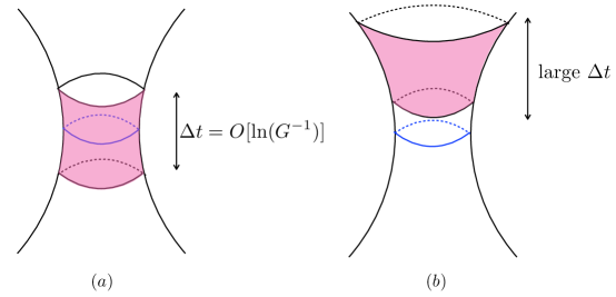
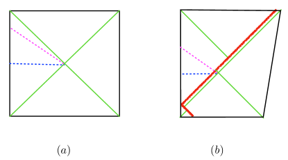
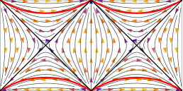
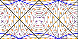
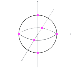
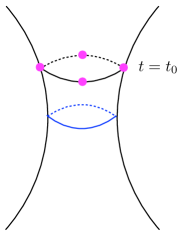
As we will see, the accuracy of this approximation is far from uniform across the de Sitter background. Instead, it is typically best in a region near where the reference objects in the state are well-localized. The approximation then degrades as one moves to more distant regions of the spacetime. Our results also indicate that it is difficult (and likely impossible) to engineer settings where the dS QFT approximation holds to high accuracy over regions that span a global time interval of more than that is symmetric with respect to the past and future of global de Sitter or, more generally, which contains a minimal that we may call ; see figure 1 (a). On the other hand, because such minimal spheres describe the most fragile regions of global dS, we find that we can nevertheless obtain a good approximation to dS QFT over arbitrary spans of global time, so long as we take the associated regions to be far to the future (or far to the past) of the associated minimal ; see figure 1 (b).
It will be useful to begin by describing the Hilbert space of gauge-invariant states on which the operators (1.5) will act. We review this construction in section 2.1, using the group-averaging construction of Higuchi_1991 ; Higuchi_1991_2 . We then apply this formalism to dS1+1 in Section 3. While Einstein-Hilbert gravity is trivial in two-dimensions, it is nevertheless useful to analyze dS1+1 as a toy model of the higher dimensional cases444While one can also study dS1+1 in Jackiw-Teitelboim (JT) gravity, the JT dilaton always breaks the de Sitter isometry group to a smaller (one-dimensional) group. However, constructions analogous to those below could be studied for the case where the remaining gauge group is noncompact.. We first consider a reference state for which the classical limit describes having a single particle in each of two complementary static patches. We identify the regions of spacetime in which the dS QFT approximation breaks down, and we estimate the size of the region in which the dS QFT approximation holds. We then introduce additional reference particles, localizing at additional events, such that these events all lie on a single pair of antipodally-related timelike geodesics. However, we find that the size of the allowed region remains the same (or becomes slightly smaller). We then demonstrate analogous results for higher dimensions in section 4, before finally arguing in section 5 that dropping the requirement of time-symmetry does in fact allow us to approximate dS QFT well over arbitrary intervals of global time (so long as they are sufficiently far to the future or past). We then conclude in Section 6 with comments on cosmological interpretations of our results and outlook for the future.
2 Group averaging and perturbative dS gravity
In a perturbative analysis of any quantum theory, one expands both the operators and the quantum states in powers of a small parameter . The expansion is typically performed about a background classical solution , in which case the leading term in any quantum state is generally expected to be a state of the linearized theory around . However, subtleties arise when the background leaves some of the gauge symmetries unbroken.
The issue can be explained simply by using the Hamiltonian formalism of the classical theory. In this formalism, the phase space is subject to constraints which generate gauge transformations by taking Poisson Brackets. When leaves a gauge symmetry unbroken, there will be a corresponding constraint such that all Poisson Brackets vanish at (regardless of whether is gauge invariant). This is of course equivalent to requiring all first order variations to vanish at ; i.e., is a stationary point of .
As a result, the leading term in the equation of motion is of second (quadratic) order at . In particular, when passing from linear to quadratic order in perturbation theory, one encounters this new equation of motion even though it has no analogue in the linear theory. Such new quadratic equations of motion are called linearization stability constraints. This terminology refers to the fact that solutions to the linearized theory can be perturbatively corrected at higher orders of perturbation theory only if they satisfy such constraints. Solutions of the linearized theory that fail to satisfy such constraints are simply spurious and do not represent linearizations of solutions to the full theory. See e.g. Deser:1973zza ; Moncrief:1975 ; Moncrief:1976un ; Arms:1977 ; Arms:1979au for discussion of such issues in classical general relativity.
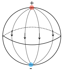
A classic example of this phenomenon occurs in Maxwell theory coupled to charged fields on (where the factor is the time direction). The linearized theory will admit general linearized solutions for the charged fields. But since the charge-density is typically quadratic in the charged fields, at quadratic order the charged fields will source the Maxwell field. And since has no boundary, there is no way for electric flux to leave the sphere. As a result, the Maxwell Gauss law requires the total electric charge to vanish; see figure 2. It is thus only linearized solutions with vanishing net electric charge that can be linearizations of solutions to the full theory.
In the Maxwell example above, it is straightforward to impose the linearization stability constraints at the quantum level as well. After constructing the states of the linearized theory, one need only truncate that Hilbert space to the sector with vanishing total charge. Charge conservation then prohibits such states from mixing with the states that have been discarded. Since no new constraints arise at higher orders, we can then proceed to arbitrary orders in perturbation theory without further obstacles.
The gravitational case is qualitatively similar in many ways. Consider in particular gravitational perturbation theory around global dSD. The SO isometries are unbroken diffeomorphisms and, since the Cauchy surfaces of global dS are compact, all diffeomorphisms are gauge symmetries. The associated SO generators must therefore vanish and, at quadratic order, this simply sets to zero all de Sitter charges of the linearized theory. At the classical level it is then straightforward to select linearized solutions with vanishing charges and to correct them at higher orders.
However, a subtlety arises in the quantum theory. Since SO is non-compact, the spectra of its generators are generally continuous. As a result, in the linearized theory, the only normalizable state with vanishing SO charges is the de Sitter-invariant vacuum . Restricting to this state would then forbid the study of any excitations at all.
Nevertheless, a so-called group-averaging approach to constructing a larger Hilbert space for the perturbative theory was described by Higuchi in Higuchi_1991 ; Higuchi_1991_2 . In essence, the idea is to first note that the linearized theory does contain states with vanishing charges, though they are non-normalizable555As described in Chen:2024rpx , these non-normalizable states may be better thought of as well-defined weights on an appropriate algebra.. Since states that are annihilated by the de Sitter charges must be invariant under the de Sitter group, we will henceforth refer to these as de Sitter-invariant states. It turns out that one may then usefully renormalize the inner product of the linearized theory to yield a well-defined Hilbert space of de Sitter-invariant states satisfying the linearization stability constraints. We will refer to this as the Hilbert space of linearized perturbative gravity in the expectation that each state in is indeed the linearized description of a state in the full quantum gravity theory.
In particular, we will see that operators of the form (1.5) are densely defined on . The general theory of the Hilbert space has been discussed in Marolf:1994wh ; Marolf:1994ae ; Ashtekar:1995zh ; Giulini:1998rk ; Marolf:2000iq under a variety of names. It will be reviewed briefly in sections 2.1 and 2.2 below, after which we analyze special observables of the form (1.5) in section 2.3. It is useful to mention that the group averaging construction has also been called the method of coinvariants in Chandrasekaran:2022cip ; Chen:2024rpx . See also Chakraborty:2023los for a recent discussion of such constructions in the context of the gravitational path integral.
2.1 Review of group averaging
It is natural to expand perturbative quantum gravity in powers of . As a result, the first-order theory will consist of linearized gravitons together with a matter quantum field theory on a fixed de Sitter background. As mentioned above, we refer to the Hilbert space of this matter-plus-graviton theory as . The matter quantum field theory can in principle be strongly coupled, though we will restrict to free theories below for simplicity.
The group averaging construction of Higuchi_1991 ; Higuchi_1991_2 can then be described as follows. For a state , consider the formal integral
| (2.1) |
where is the orthochronous de Sitter group SO, gives the unitary representation of , and is the Haar measure on . Since is non-compact, the states are not normalizable using the standard inner product on . Let us therfore introduce a new group-averaged inner product,
| (2.2) |
which removes one integration over . The inner product (2.2) thus effectively divides the old inner product by the (infinite) volume of the de Sitter group. The Hilbert space of de Sitter invariant states (which provide the linearized (L) description of valid perturbative gravity (PG) states) is then defined by choosing a useful linear space of states with finite group-averaged inner products (2.2) and completing the space spanned by their linear combinations (modulo null states).
We note that the expression (2.1) plays only a formal role in this construction and that one may alternately consider (2.2) as a new inner product on the original states . With respect to this new inner product, states of the form are null states for all . Using this description of the group-averaging inner product, the above construction was called the method of coinvariants in Chandrasekaran:2022cip ; Chen:2024rpx .
The group-averaging construction is useful when results in a finite and positive semi-definite inner product (2.2). Since (2.2) clearly diverges for a de Sitter-invariant vacuum , our can only contain states orthogonal to . This is not to say that there can be no well-defined state of quantum gravity associated with , but merely that the inner product on should not be renormalized. Furthermore, since is the unique normalizable de Sitter-invariant state in , any well-defined de Sitter-invariant operator whose domain includes can only map to a multiple of itself. Thus such observables cannot mix the state with states defined from the above domain . As a result, unless one has good reason to introduce additional de Sitter invariant observables, it suffices to treat separately from all other states; see Marolf:1996gb for general discussion of this issue.
In a theory with well-defined particle number (say, in the sense of being positive frequency with respect to global time), one might thus like to find that (2.2) is both finite and positive definite for a natural space that is dense in the space of states with particles. As explained in appendix A, the full story is more complicated, and there remain holes in the existing literature associated with light scalar fields and fields with spin. However, at least for gravitons on dS3+1 and for scalar fields in any dimension with mass , there is strong evidence that the above is essentially correct, though there are three subtleties.
The first subtlety is that, as written, (2.2) is in fact ill-defined for particle states but, as explained in A, one should nevertheless define it to be zero for such states. This result is the natural quantum analogue of the observation that single point-particles in dS always have at least one non-vanishing dS charge and, as a result, that a single particle never satisfies the linearization stability constraints described in the introduction. It would be interesting to understand whether this feature might be related to complications described in Chandrasekaran:2022cip when they attempted to introduce an observer in only one static patch.
The second subtlety is that two-particle states again have divergent group-averaging norm. As described in appendix A, this appears to be associated with the fact that all classical 2-particle configurations with vanishing dS charges continue to leave a non-compact subgroup of SO unbroken and, as a result, well-defined de Sitter-invariant operators again cannot cause 2-particle states to mix with standard Fock states having particles.
Finally, the third subtlety is that, while positivity for -dimensional linearized gravitons was checked explicitly in Higuchi_1991_2 , there is not yet a complete proof that the group averaging inner product is positive semi-definite for all states of particles of scalar fields with the masses indicated above. See appendix A for discussion of the current status of this issue.
2.2 Group averaging with a Reference
Let us now divide our de Sitter QFT into a target system and a reference system. For simplicity we will assume that takes the form of a tensor product,
| (2.3) |
where describes a system to be used as a reference and describes the target system whose physics we wish to more actively probe. We will imagine that, before imposing de Sitter invariance, the system induces a definite pure state , so that we need only consider states of the full system of the form for some . Group averaging such states produces de Sitter-invariant states of the form
| (2.4) |
which then live in the space of allowed states for perturbative gravity (PG) at order (at which the gravitational theory is linear (L)). We will use to refer to the Hilbert space defined by states of the form (2.4) using the group-averaging inner product.
We expect to be able to take a limit in which serves as a sharp reference within our de Sitter space, and with respect to which at least certain observables can be well-localized. For example, for the right fields, and in the correct limit, could describe a very classical planet Earth equipped with all manner of laboratories and marked reference points with respect to which one could classically construct relational gauge-invariant observables (e.g., the average value of the Higgs field in the city of Paris during the opening ceremonies of the 2024 Olympics). We therefore expect that, under the right conditions, we can also construct relational quantum observables which are well-described by local quantum field theory on a fixed de Sitter spacetime.
Before turning to the observables themselves, it is useful to further investigate the Hilbert space structure associated with the states (2.4). The group-averaging inner product of two such states takes the form
| (2.5) |
The expression (2.5) is a convolution over the group of a state-dependent factor and a factor that will remain fixed so long as our reference system is undisturbed. We will refer to the fixed factor as the group averaging kernel.
If there were a normalizable state for which this kernel was a Dirac delta-function, , then the inner product (2.5) would reduce precisely to the inner product on , i.e. we would have . While this seems unlikely to be the case for any normalizable state, it is nevertheless true that for any state with absolutely-convergent group-averaging norm
| (2.6) |
the appearance of this group-averaging kernel in (2.5) will tend to localize the integral over to a region surrounding the identity. This follows from the fact that, since is unitary, we must have with equality only for . Furthermore, if (2.6) converges absolutely, then the kernel will suppress contributions far from the identity.
Of course, this region may be very large for a general state . But we will study limits in which becomes sharply peaked, so that the associated region is small. The inner product (2.5) will then be given by the usual dS QFT inner product on with small corrections associated with the finite width of the peak of .
We will characterize these corrections more precisely in sections 3 and 4 for particular choices of reference state . In particular, we will see there that the associated corrections to correlation functions are not uniformly small across the entire de Sitter space, but that their size depends on the location of the arguments of such correlators in relation to structures defined by .
Let us now consider the case where and describe independent local quantum fields with no mutual interactions. For the moment, we will still allow both and to have self-interactions. Furthermore, we can in fact allow to denote a collection of mutually-interacting quantum fields, and similarly for , so long as the fields of and the fields of do not interact with each other666We expect that the inclusion of perturbative interactions between the and will be straightforward, but we will not pursue it here. We thus see no obstacle to including linearized gravitons in either or ..
2.3 Relational Observables for perturbative dS gravity
Since operators can be built from bra- and ket-states, and since limits where is sharply peaked make canonically isomorphic to , we should also expect there to be an algebra of gauge-invariant (i.e., de Sitter-invariant) observables that reduces in this limit to the algebra of local -fields. The construction we will use is a direct analogue of our construction (2.4) of quantum states. Given a local field that acts on , for any point in global dS we simply define the operators
| (2.7) | |||||
| (2.8) |
where denotes the image of the point under the de Sitter isometry . Note that, even for a fixed value of , we can use the fact that the Haar measure is invariant under to write . The operators (2.8) are thus de Sitter-invariant and represent observables of the linearized perturbative gravity (LPG) theory for each fixed value of .
As foreshadowed in the introduction, this construction makes use of non-local elements both in the integral over the group of de Sitter isometries and also through the explicit use of the global quantum state . This feature will play a critical role in ensuring that the operators (2.8) are well-defined and, in particular, that they have finite matrix elements between states of the form (2.4). Such matrix elements are computed by applying the operators (2.8) to a state and then taking the group-averaging inner product with . Recalling the definition of our states (2.4), and since the group-averaging inner product (2.5) removes one of the integrals over the de Sitter group, the result then takes the form:
| (2.9) |
Convergence of the integrals in (2.9) is guaranteed by the absolute convergence of (2.6). Again, it is manifest that (2.9) reduces to the correlators of dS QFT in limits where our group-averaging kernel approaches .
In the particular case where either or is the de Sitter-invariant -vacuum , the factor of can be dropped from the final line. Since it will be natural to focus on this case below, we define the notation
| (2.10) |
Thus we may also define
| (2.11) |
However, we emphasize that the state (2.10) is only vacuum with respect to , and that the field is in a group-averaged version of the state . In particular, the state defined above still contains our reference and is thus not the vacuum of the full perturbative gravity theory. It will thus induce non-trivial backreaction at higher orders in .
Since states with absolutely-convergent group-averaging norm will define group averaging kernels with finite width, choosing some of the points to lie on each other’s light-cones will cause (2.11) to differ infinitely from the corresponding correlator in dS QFT. However, this strong difference is clearly associated with very high energies. It is thus useful to describe the manner in which (2.11) approximates correlators of dS QFT by studying smeared correlators (which are sensitive only to the physics below an energy scale set by the smearing function). For example, in a free theory it suffices to study smeared two-point functions of the form
| (2.12) |
for appropriate smearing functions . We will focus below on the case where are members of a family of functions that are well-approximated by Gaussian functions of both the global time and of the location on the sphere at fixed that are peaked at the point in global dS. We will take the width of these Gaussians in both global time and in location on the sphere to be identical as measured in terms of proper time and distance. For example, when lies at the north pole of the sphere at some time , and for an appropriate normalization factor we may take
| (2.13) |
where are the global coordinates of the point with being the polar angle on , and where the final approximation holds for . We note for future reference that the final exponent on the right-hand-side defines an effective flat Euclidean-signature metric with line element
| (2.14) |
so that
| (2.15) |
where is the Euclidean distance between and defined by777The astute reader will note that, if we wish to define for general away from the north pole by rotating (2.13), then the analogue of (2.14) in fact depends on the location of on the sphere . While this fact is not explicitly indicated by the notation , it will not play an important role in our analysis. (2.14).
We also note that the effect of convolving smeared dS QFT correlators with our group averaging kernel will depend on the extent to which differs from , and thus the extent to which the exponent on the right-hand-side of (2.13) differs between and . Since the triangle inequality bounds the change in in terms of , we see that for the change in the smearing function is small when .
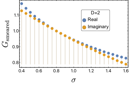
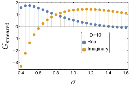
The question of whether this small change in the smearing function can cause a significant change in smeared correlators can be studied by using a standard partition of unity to divide the domain of integration into subregions based on whether subsets of the are close together or far apart. For example, when studying the smeared two-point function (2.12), we divide the domain of integration into a region with (Lorentz-signature de Sitter distance) and regions with and . In the former region, the integral is well-approximated by a smeared Minkowski-space correlator. Since the Wightman axioms require Minkowski-space correlators to be tempered distributions Streater:1989vi , and since tempered distributions are continuous linear functionals on the space of test functions, the integral over this region will change by only a small amount under a small change in the smearing functions . Here it is important to that we consider Wightman correlators rather than their time-ordered counterparts. Similar continuity follows for the integral over the regions and since the correlator is bounded in those regions and the smearing function changes by a function of integrable norm; (i.e., by a function in )888For free fields on dS, one may alternatively proceed by writing the field operator as an expansion in global dS mode functions that solve the equation of motion. Integrating any given mode against a smooth function of time yields a result that must vanish faster than any polynomial as the angular momentum of the mode becomes large. It thus follows that the relevant mode sums converge absolutely. The desired result then follows from the fact that the above convolution makes negligible change in the high-frequency components of .. Inserted: This continuity is illustrated by the numerical examples in figure 3. As a result, when for all within the peak of the group-averaging kernel, a given set of smeared dS QFT correlators will be well-approximated by the correspondingly smeared versions of the perturbative gravity correlators (2.11).
3 Reference states in dS1+1
The above section described our general framework for using perturbative gravity to approximate the algebra of local observables in dS QFT. There we saw that a central role is played by the group averaging kernel , and that comparison of the perturbative gravity and dS QFT correlators is controlled by i) the width of the peak of about the identity and ii) by the effect of those isometries that lie within the above peak on the points at which we wish to evaluate such correlators.
We thus now turn to a detailed investigation of this kernel for interesting classes of states. In this section we consider the simple-but-illustrative case of global de Sitter, taking the field to be a collection of free scalar fields with mass (so that the one-particle states lie in principal series representations of SO VK ; Wong:1974cv ). Thinking of as a collection of fields allows us to choose each particle to be associated with a distinct scalar field. We may thus treat the -particles as distinguishable, which provides a slight simplification of the calculations. While Einstein-Hilbert gravity is trivial for the case , our goal is to use as a toy model of higher dimensional physics. We thus simply analytically continue certain formulae from higher dimensions to in order to discuss versions of linerization stability constraints (which are again solved by group averaging), perturbative gravity operators, and a (dimensionless) Newton constant . However, we will postpone any more involved discussions of back-reaction to section 4 (where the higher-dimensional case will be addressed).
3.1 Preliminaries
Studying our kernel requires an understanding of how the de Sitter isometries act on our states. It is useful to begin by recalling that, in global coordinates, the metric on dS1+1 takes the form
| (3.1) |
where is the de Sitter scale. It will sometimes also be useful to write the metric in conformal coordinates , where with , so that the line element becomes
| (3.2) |
In these coordinates, the generators of the isometry group are
| (3.3) | |||
| (3.4) | |||
| (3.5) |
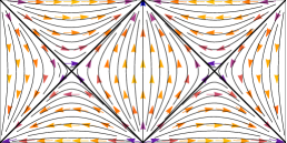
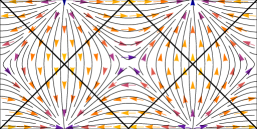
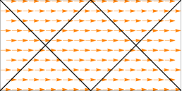
where the notation , , classifies the generators of SO according to their action as either boosts or rotations when one thinks of SO as Lorentz transformations on 2+1 Minkowski space. The actions of these Killing fields on de Sitter space is shown in Figure 4 below.
The action of the generators on our states can be understood by defining
| (3.6) |
We then have the commutation relations Sun:2021thf .
| (3.7) |
The Casimir operator is given by
| (3.8) |
We now let be the 1-particle eigenstate of the operator with , where is an integer. In particular, we may take it to be the state created from the -vacuum by acting with the creation operator associated with the usual mode of the scalar field having angular quantum number . For one-particle states, the Klein-Gordon equation gives , where is the mass of the scalar field and where we consider only the case . It will be useful to introduce the parameter through
| (3.9) |
By convention, we take the imaginary part of to be positive, so that we have . It is then straightforward to check that we obtain a unitary representation of the above relations by imposing
| (3.10) | ||||
| (3.11) | ||||
| (3.12) |
Below, we will also use the notation
| (3.13) |
Let us now conclude our discussion of preliminaries by reviewing the results of Marolf_2009 describing the asymptotics of the kernel at large . For this purpose we will in fact consider scalar fields of any mass , where we take to be defined by (3.9) with the convention that for . We will take to be an -particle state and, for each particle, we take the state to be a finite linear combination of the above states .
The results of Marolf_2009 were expressed by writing a general in the form . Since range over a compact space, and since the resulting rotations simply map any given angular momentum mode to a superposition of other such modes, the large behavior is controlled by the behavior of at large . And since de Sitter isometries act diagonally on multi-particle states, our group averaging kernel will contain factors of for each particle, where again denotes an angular quantum number. At large , the asymptotic behavior of this 1-particle matrix element was shown to be
| (3.14) |
so that the group averaging kernel decays exponentially with large boost parameter. Since the relevant integration measure for dS1+1 is (see again Marolf_2009 ), we see that (2.6) converges absolutely for . In particular, for we require . As discussed in Marolf_2009 , this is also the case for scalar fields of mass in for any .
3.2 A pair of reference particles on opposite sides of dS
Having seen that our kernel strongly suppresses contributions from large for particles with , we can now turn our attention to the region near the identity at which the group-averaging kernel is peaked. Though one can certainly engineer special cases where there are also important contributions from outside this peak, having a second peak of height near clearly requires fine tuning. Furthermore, if the height of another peak is not near , a different form of fine tuning is required if its contributions are to be comparable to or greater than those of the unit-height central peak. Since we do not expect this to occur for generic , we will defer consideration of this possibility until introducing the particular states we wish to study. At that point, we will display numerical results supporting the above expectations.
For the moment, however, we will simply compute the width of the central peak for interesting classes of states by writing and expanding to second order in . We will in fact focus on the simple case of 2-particle states (with ). As noted above, to control contributions from large the full state must contain a third particle. But we are free to choose the state of the third particle to have a much broader peak near the identity (perhaps engineered by smearing an arbitrary state over a large-but-finite range of de Sitter transformations), so that the width of the kernel is set by just the first two particles.
At the classical level, a pair of identical-mass particles can satisfy the linearization stability constraints in only if their de Sitter charges cancel exactly. This requires the geodesics followed by the two particles to be related by a rotation through an angle for some rotation generator. We will take this to be the rotation . We will thus choose a quantum state for the first particle and then simply take the state of the second particle to be
| (3.15) |
with the full 2-particle reference state being the tensor product
| (3.16) |
Rather than attempt a general classification of the possible such states , we will confine our investigation to a simple choice that facilitates explicit calculations. We take the first particle to be localized around , so that the other is then localized around . In particular, we take to be of the form
| (3.17) |
for some cutoff , where the coefficients are found by expanding Dirac delta-functions and in terms of rotational harmonics . This is a convenient choice, since Equations (3.10)-(3.12) give the action of all generators on these eigenstates. As , the particles become perfectly localized at the points at time . Numerical plots showing that the group averaging kernel defined by this state from a tight peak around the identity (with small secondary peaks) are shown in figure 5.
[width=]figures/GAkernel
Since the magnitude of our kernel is greatest at the identity, we can study the width of the peak by expanding to quadratic order in and . To this order, the kernel is then determined by the expectation values of and the expectation value of symmetrized products of pairs of generators. However, many of these moments vanish even in the state since is invariant under (which as shown in figure 4 maps to ). Using to denote the expectation value of an observable in the state we thus find
| (3.18) |
so that the only non-vanishing moments in at this order are , , , , and . Furthermore, since is invariant under the rotation (which as shown in figure 4 maps to ), the contributions to and from must cancel against each other.
We first consider the case where (and ). We may then use the approximation . Direct computation shows that
| (3.19) | ||||
We may also consider the case when . Using the approximation , we find
| (3.20) | ||||
Let us therefore introduce the parameters , , , in order to write the group averaging kernel as an approximate Gaussian
| (3.21) |
where we emphasize that for all . The widths of the peak in the various directions are then proportional to and, in the limit, the Gaussians become proportional999Since we have chosen to be normalized, we will always find . So, as written, the limit gives a delta-function with a vanishing coefficient. However, for the same reason, the norm also vanishes in this limit for any normalized . Obtaining normalized states thus requires taking to scale as . Combining this factor with the Gaussian (3.21) yields the desired delta-function. to a delta-function that sets for all . In this limit, the inner product between two physical states reduces to the standard QFT inner product without additional smearing.
However, the large limit requires and/or to become large. In the presence of dynamical gravity, either option would induce a large gravitational backreaction. Hence the must remain bounded if we wish to keep such backreaction small. We will characterize this backreaction more precisely in section 3.2.1 below.
3.2.1 Characterizing backreaction
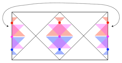
In order to estimate the bounds imposed on the associated with the restriction to small backreaction, we will need to say more about how this backreaction will be measured. Gravitational backreaction on -dimensional de Sitter space is generally highly non-uniform, so that for any classical perturbation of dS one can find some sense in which the backreaction is large. This is perhaps most simply illustrated by making use of the Gao-Wald theorem Gao:2000ga , showing that any perturbation satisfying the null energy condition forces the past (or future) of any timelike geodesic to contain a complete Cauchy surface. There is thus a sense in which applying a large boost to any spherical cross-section of the perturbed de Sitter space must give a Cauchy surface of vanishingly small total volume; see figure 6. This is in sharp contrast to the case of unperturbed dS, where applying any dS isometry to the at of course exactly preserves its finite volume.
We will choose to measure the backreaction near the round that passes through the spacetime points at which our particles are well-localized; i.e., the at with the coordinates and states defined as above. As discussed in Giddings_2007 , a reasonable measure of the backreaction in this region is the total flux of energy through this , where
| (3.22) |
in terms of the QFT stress tensor , the unit normal to the surface , and the volume element of the induced metric on this surface. If we wish to keep the level of backreaction on the geometry below some fixed cut-off, then in terms of the bulk Newton constant , the maximal allowed value of will of course scale as in the limit . While Einstein-Hilbert gravity is not dynamical in 1+1 dimensions, we can nevertheless use our investigation of dS1+1 as a toy model of the higher-dimensional case by introducing a (dimensionless) parameter and imposing the restriction
To understand the constraint this imposes on our , we will need to estimate the contributions to arising from the mass and angular momentum of our -particles. This is straightforward due to the fact that the time derivative of the metric vanishes at . As a result, the local notion of positive-frequency mode near associated with the standard definition of particles in global de Sitter coincides with the notion of positive frequency for the static cylinder metric
| (3.23) |
Our thus coincides with what one would call the energy on the static cylinder (3.23) when computed in terms of the angular momentum . It is thus clear that, If both particles were in modes having angular momentum precisely , we would find
| (3.24) |
In order to limit backreaction, we must thus take the mass parameter and the maximum angular momentum to satisfy and as .
Let us first we examine the ultrarelativistic limit (, though with ). The results (3.19) then simplify significantly to yield
| (3.25) |
We see that the dependence on disappears at leading order in .
As described in section 2.3 the effect of group averaging on correlation functions smeared with the global coordinate near-Gaussians of (2.13) will be small when the smearing is confined to de Sitter isometries such that
| (3.26) |
where is the flat Euclidean distance defined by (2.14) and we consider all located within the peak of each near-Gaussian . Since the Gaussian (3.21) gives significant weight only to group elements with , for large-but-finite the condition (3.26) is equivalent to
| (3.27) |
where is the Euclidean norm of the appropriate vector field from (3.3)-(3.5). In particular, we have
| (3.28) | ||||
| (3.29) | ||||
| (3.30) |
In regions of spacetime where any of the bounds (3.27) are exceeded, the spacetime resolution of the observables is low, and the dS QFT approximation to perturbative gravity breaks down even for correlators smeared with the functions (2.13). The corresponding cutoff contours (at which ) are shown in Figure 7 for specific values of and . At sufficient depth within the region between these contours, dS QFT correlators smeared with the function (2.13) will be well-approximated by correspondingly-smeared perturbative gravity correlators.
[width=0.4]figures/allowed_region
Note that at large we have . As a result, consulting (3.29) and taking large as well, we see that over most of the spacetime the large cutoff will be set by
| (3.31) |
However, this bound diverges when . In particular, in the static patches associated with the geodesics the Euclidean norm of satisfies . In such regions the bound is thus set by either or . Since the Euclidean norms of and are nearly identical at , at late times (3.19) gives , while the cutoff is in fact instead set by . In such regions we thus find
| (3.32) |
So, for , the ultrarelativistic limit yields a good approximation to dS QFT only for global times , though the actual cutoff becomes at . As a result, the spacetime volume of the region where our approximation is good is of order .
We can now return to (3.20) and consider the case . If we take e.g. and as , we find but In contrast, if we take but with , then we find and . We can also set all 3 coefficients to be the same order in by choosing and , in which case we find . Any of the above cases will again confine the region in which our dS QFT approximation is accurate to one which spans a global time interval of order with a coefficient of order . We will therefore confine attention to the simpler ultrarelativistic case below.
3.3 Adding more reference particles
For the above reference state, we found that smeared dS QFT correlators are well-approximated by our smeared perturbative gravity correlators only in a region of de Sitter space spanning global times of order . It is thus interesting to explore whether this region can be enlarged by considering a more complicated reference state. We are particularly motivated by a desire to understand whether the region can be enlarged within a natural static patch of dS, perhaps at the expense of shrinking the allowed region outside. In this section, we investigate the effect of adding additional reference particles localized at points along the and geodesics.
As before, it will be useful to keep the full reference state properly ‘balanced’ in the sense that it has vanishing expectation values of to avoid giving de Sitter charges that are parametrically larger than those of the -system (as that would then require group averaging to nearly annihilate the resulting state in order to extract a state in which the total de Sitter charges vanish).
We will consider states of the form with , but where now contains three particles that become well localized along the geodesic at times , , and . In particular, we take
| (3.33) |
where is again given by (3.17). Thinking of as the static patch Hamiltonian, we see that moments of in the various one-particle states will be given by moments of static-patch time-translations of in . It will thus be useful to compute expectation values like
| (3.34) |
where is a linear or quadratic expression in . For or , the time translation has no effect and (3.34) reduces to matrix elements calculated previously. For and , it is useful to define operators corresponding to lightlike (null) rotations which have commutation relations
| (3.35) |
As a result, under a time translation, these operators satisfy , from which we obtain the time translations of and :
| (3.36) | ||||
| (3.37) |
We can now use the above results to compute the group averaging kernel. Since our new still enjoys the symmetries discussed near (3.18), the moments listed in (3.18) once again vanish. It thus remains only to compute expectation values of , , and . These moments receive contributions from the corresponding moments of each 1-particle state. The expectation value of also receives contributions from cross terms between various pairs of particles, associated with the fact that is non-zero in all one-particle states. Other cross terms vanish since The final result for our kernel is thus
| (3.38) |
where again refers to the expectation value of in .
For , these coefficients are given by
| (3.39) | |||
| (3.40) | |||
| (3.41) |
As in the two particle case, the QFT approximation holds exactly in the limit . The coefficients still grow with increasing , but now they also grow with increasing .
Let us thus investigate how large we can take while keeping the backreaction small as measured by (3.22); i.e., for . Recall that gives the total energy that the state would have if it were placed in a static cylinder spacetime of radius (keeping the state unchanged in the Fock basis defined by angular momentum modes). The particles at will contribute to according to (3.22) as they did before. However, the contributions of the time translated particles are easiest to study by evolving the particles from to .
For the particles that localize at , it is convenient to perform this evolution using the description provided by the static patch centered at . The time translation from to is then trivial but, as we evolve them back to , the particles move to higher energies as they fall away from toward the static patch horizon.
Let us first consider the limit so that the particles are relativistic, and so travel along null rays. Such particles rapidly approach the de Sitter horizon and then blueshift exponentially with respect to the vector field in (3.22). We thus find that the total flux of energy through is
| (3.42) |
where the final right-hand-side gives the leading behavior at large and .
At leading order in and we also find
| (3.43) |
The cutoff contours will look very similar to the ones we found before, except that there is now an extra parameter to vary. Outside the static patch, we expect the cutoffs to again be set by since it remains of order (since particles related by static-patch time-translations must contribute equally to ). Inside the static patch, estimating the cutoff time using either or and setting leads to
| (3.44) |
so that we again find for any allowed choice of . We thus see that, with a given finite energy budget measured by , adding localized particles along the geodesics fails to increase the size of the allowed region.
While we have not investigated other choices of reference states in detail, the exponential increase of kinetic energies with static patch time is typical of any particles falling toward a de Sitter horizon. This suggests that the above behavior is generic when we require backreaction to be small at for our global time ; i.e., at a minimal . For example, the same exponential factors arise in the nonrelativistic limit . However, in section 5 we will explore the possibility of allowing backreaction at such minimal spheres to be large, and thus allowing to be large, while requiring backreaction to be small in other regions of de Sitter space. Due to that fact that it will require a slightly more involved discussion of backreaction in Einstein-Hilbert gravity, and since our discussion of ‘backreaction’ for was simply a convenient fiction designed to provide a toy model of well-known results for Einstein-Hilbert gravity in the higher dimensional case, we postpone that discussion to section 5 and, in particular, until after treating group averaging in higher dimensions in section 4.
4 Reference states in dSd+1
We will now see that essentially the same results found above for also hold for dSD with . We begin with a discussion of particle states and the associated action of SO generators following Marolf_2009 . To this end, we consider a sphere , with metric
| (4.1) |
where is the polar angle and we use coordinates . In global dS we use the corresponding global coordinates (with global time ) in which the metric takes the form
| (4.2) |
Bosonic one-particle wavefunctions on can be written in terms of spherical harmonics labelled by angular momentum vectors with for . For , we take to be the total angular momentum quantum number for the SO subgroup of SO associated with the sphere at constant for . The above quantum numbers thus satisfy
| (4.3) |
In analogy with the construction in section 3.2, we begin by considering a reference state where each state describes a particle that is well-localized at at one of the poles of the . For simplicity, we take each particle to be invariant under the SO rotations that preserve the poles. As a result, two particles will not suffice to break all of the dS isometries, so we will need to add more particles later. Indeed, we will soon define , where the for are constructed from by applying rotations by in orthogonal directions; see the discussion below.
In the state , the only non-zero angular momentum will be , for which we henceforth use the simplified notation . We will again consider a free scalar field with 1-particle states in the principle series, with . We take the state of each particle to be of the form
| (4.4) |
where denotes a particle at the north pole and denotes a particle at the south pole, and where is a normalization constant.
The coefficients will be given by the spherical harmonic expansion of an Dirac -function localized at the relevant pole. It is natural to write this delta function in the form
| (4.5) |
where is the standard Dirac delta-function associated with the measure and is the volume of the unit -sphere. There is an analogous result for the -function at the south pole. The -dimensional spherical harmonics for are given (see e.g.Marolf_2009 ) by
| (4.6) |
where there is no dependence, since the associated harmonic simplifies to . The other harmonics are given by
| (4.7) |
and by
| (4.8) |
where we see the above are independent of . Thus the relevant spherical harmonics depend only on . We can now determine the coefficients in the expansion of and in terms of the spherical harmonics noting that, since we will normalize the answer afterwards, we care only about the -dependent factors. We find
| (4.9) |
With these coefficients, the normalizations for the states are
| (4.10) |
The generators of the de Sitter group consist of the rotations about each spatial direction (with and ), and boosts . It is convenient to use the embedding space formalism to find the expressions for the corresponding Killing vector fields in terms of global coordinates. In this formalism, we represent our de Sitter space as the hypersurface in a -dimensional Minkowski space with metric . On the hyperboloid, the Minkowski coordinates are then related to global coordinates through , , where the are functions of the angles on that define the standard embedding of in ; e.g. , , etc. The Killing fields are thus
| (4.11) | ||||
| (4.12) |
Note that the action of is the same as in dS1+1 given by Eq. (3.3), but with replaced by and with (3.4) rewritten in terms of global coordinates.
As in Section 3, we use the above description of to compute the group averaging kernel to order in order to determine its width around the identity. The calculation of the kernel is greatly simplified by the symmetries of our reference state. First, vanishes for , since these rotations have no effect on scalar particles at the poles. Second, the expectation values of all rotation generators also vanish, and so too will the expectation values of all for due to the invariance of our states under reflections. In particular, the states are each individually invariant under reflections defined by choosing some and mapping while holding fixed all with . Additionally, under the reflection , the generator transforms as . This leads to a cancellation between the remaining terms of order (since the only such terms were those associated with the expectation value of ).
Finally, we consider the cross terms , , , and , for , and where the expectation values are taken in either the or state. That these all vanish can be seen by applying the reflection symmetries , under which each of the above combinations of generators picks up a sign, but under which the states are individually invariant. Due to the above vanishing moments and cancellations, the group averaging kernel defined by becomes just
| (4.13) |
The analysis of the above coefficients is somewhat tedious. We therefore relegate the details to appendix B and merely quote the leading results at large from (B.18):
| (4.14) | ||||
| (4.15) | ||||
| (4.16) |
It is reassuring to note that for the results (4.14) match exactly with (3.19).
The exact zeros of for are due to the fact that – for simplicity – we chose our state to preserve certain rotational symmetries. Similarly, the small values of are due to the fact that our particles are localized near the corresponding horizons, so that they also preserve those symmetries at leading order.
However, as noted above, we wish to add additional particles to break these symmetries. It is convenient to take the additional particles to be obtained by taking the above pair of particles (which localize along the axis) and rotating them so as to instead localize along the th axis. In particular, for , we define the 2-particle states . We then combine the above states to construct a state
| (4.17) |
now with particle number such that each particle is localized at along a different positive or negative axis in the embedding space ; see figure 9.
For the state (4.17) we find
| (4.18) |
with
| (4.19) | |||||
| (4.20) |
Here still denotes the expectation value of in the original state and the approximation is valid at leading order in . We see that all are manifestly positive.
By the same argument as in dS1+1, our dS QFT correlators will be well-approximated by our perturbative gravity correlators in regions where the Euclidean norms (see (2.14)) of the killing vectors are much smaller than the , . To find the relevant , we use (4.11). To find the magnitude of the in Euclidean signature, we can use (4.12), or we can make direct use of the embedding space coordinates. The results are
| (4.21) | ||||
| (4.22) |
In order to describe the region in which our dS QFT correlators are well-approximated by our perturbative gravity correlators, let us note that since is independent of , and since is independent of , the region in which our dS QFT approximation holds to any fixed accuracy will be invariant under the full SO group of rotations that preserve the global time . It therefore suffices to test the conditions only at the pole where . Furthermore, we may focus on the generators and since, for large , we see from (4.21) that all other boosts and rotations have equal or smaller Euclidean norm at . Using either or leads to the condition
| (4.23) |
where the last step extracts the leading behavior and drops coefficients of order . Thus, as in our 1+1 toy model, for , we find that our dS QFT approximation can hold only in a region spanning a global time interval of size .
5 Reference particles in future dS
In section 3.3 we found that, with a fixed energy budget measured by the flux through a minimal in dS1+1, adding boosted particles in states did not improve our approximation of the local algebra dS QFT in any region of dS1+1. Since the results in section 4 for particles localized at in are quite similar to those in section 3.2, it is again clear that with fixed total energy-flux through a minimal , adding more particles localized at other times will again fail to improve our approximation of local algebras in -dimensional dS QFT.
However, the key limitation in section 3.3 arose from fixing . Furthermore, as discussed in section 3.2.1, there is generally no sense in which backreaction can remain small across all of dS, so one must make a choice of both where, and in what sense, one wishes perturbation theory to hold. Finally, since global de Sitter space is exponentially large in both the far future and the far past, the energy carried by perturbations tends to become extremely diluted in such regions and backreaction tends to be much smaller than at a minimal .
Let us therefore investigate what we can do if we decide to allow large backreaction near the minimal at (thus dropping the constraint on ), though we will still require backreaction to be small to the future of some global time slice where the particles all localize. We will do so using the reference state
| (5.1) | |||||
| (5.2) | |||||
| (5.3) |
where are again given by (4.4); i.e., we use only particles that become localized at global time and we again impose in (4.4). At time , each particle thus gives only a small perturbation, and the perturbation toward the future should be even smaller. We will investigate later the extent to which the resulting perturbations can remain small at times .
Since each state is invariant under the same set of (spatial) reflection and rotation symmetries as the similarly-labeled state in section 3.3, the non-vanishing moments that contribute to the group-averaging kernel are again just the expectation values of and , for which will again define squared-widths and . Furthermore, while it is straightforward to compute these expectation values from the results in section 3.3, the analyses of the previous sections show that we do not in fact need the detailed forms of the results. Instead, the important point is that, due to the boost transformations of (analogous to those in (3.36)), for the particles in state and for we will find and to be proportional to for large , though and for will be unchanged by the boost.
As a result, in the full state we will find all to be proportional to for large . This will then compensate for the fact that the Euclidean norms and are exponentially large at , and it will similarly allow these vector fields to satisfy our criterion for a good approximation to dS QFT for a global time interval of order to the future of . This condition is also satisfied whenever , so long as we consider a region of dS in which backreaction is small.
It thus remains only to estimate the backreaction from our state. There are several pieces to this discussion. First, we may note that at time we have only particles on a sphere of volume , where is the volume of the unit sphere. Furthermore, by construction each particle alone has small backreaction, meaning that it can be modeled as a Schwarzschild black hole of radius much less than . As a result, for all the particles are exponentially far apart, and – in some reference frame101010For , the particle will be highly relativistic in the reference frame associated with slices of constant global time . It should then be described as a de Sitter version of the Aichelberg-Sexl solution Aichelburg:1970dh . In 2+1 dimensions there is no curvature away from the particle, and for the Aichelberg-Sexl solution decays at long distance. But in 3+1 dimensions the Aichelburg-Sexl metric grows logarithmically. Of course, curvatures still decay and, more importantly, the gravitational field is entirely confined to a shock wave in a null plane. As a result, for the vast majority of de Sitter space remains exponentially far from such shock waves and, indeed, the total probability for an object in dS to encounter such a shock wave between global time and global time is exponentially small. – the region near each particle can be modeled as a Schwarzschild de Sitter solution (again with Schwarzschild radius much less than ). In this sense the backreaction is small at unless one probes the small region very close to one of the particles. Recalling that metric perturbations can in principle be included in the field we call , such comments can be promoted to statements about gauge-invariant operators of the form (2.8) if desired.
It is important to realize, however, that there are small perturbations to de Sitter at even far away from the expected locations of the particles. Some of this effect is due to the fact that, since we cut off the mode sum defining each particle’s state at some , the particles are not perfectly localized and their wavefunctions have long tails that extend across all of de Sitter space. That, however, is a minor issue as, at large , those long tails correspond to only a tiny net probability for the particles to be far from their expected location. Furthermore, one could remove the long tails by replacing each particle by the coherent state obtained by making a unitary transformation of the -vacuum using for some compactly-supported .
While is invariant under linearized gauge-transformations, it will not be gauge-invariant at the higher orders in perturbation theory used to compute backreaction. Instead, as usual, it must be ‘gravitationally dressed’. In the present context, the only structure to which such operators can be dressed is the background itself. This is simply a set of words which means that the backreaction need not vanish in regions that are causally separated from the support of , and that one must instead solve the gravitational constraints to analyze what happens in such regions.
It is reasonable to expect that the overall effect on the expansion/contraction of the spheres will be well-approximated by smearing the particles over the sphere. By this we mean that we will simply solve the Friedman equations for homogeneous isotropic cosmologies using the homogeneous energy density that gives a flux of energy through the given sphere that agrees with the flux computed perturbatively for our particles. Since angular momentum is conserved, assuming that and are of the same order in , once is significantly less than the particles will be relativistic and we will have
| (5.4) |
Replacing our particles with a uniform energy density
| (5.5) |
and comparing this with the energy density associated with the de Sitter cosmological constant, we find that for
| (5.6) |
i.e., the backreaction from our homogeneous will be small whenever exceeds by at least a few e-folding times.
Now, since the state contains only a small number () of particles, it is clear that the actual energy density is far from homogeneous. Some of the issues involving the inhomogeneous part of were discussed above and relate to probing the local spacetime near each particle. However, additional effects arise when, e.g. by random chance, some subset of the particles finds themselves closer together than other subsets. It is then natural to model such circumstances by a that is again smooth, but where the local energy density in that region is larger than in other regions. Comparing with our analysis above, we see that this will then increase the backreaction in such regions, though this can only be the case in small regions of spacetime. Qualitatively, then, this is similar to the comments above about probing small regions near each particle. In this sense, then, we expect backreaction to be small over the vast majority of the region of our de Sitter space at global times
| (5.7) |
As a result, our perturbative gravity correlators will be a good approximation to our dS QFT correlators over the vast majority of the region satisfying
| (5.8) |
Taking , then yields
| (5.9) |
Taking large (say, with and small but with large) then allows us to make our approximation highly accurate over a region with arbitrarily large spacetime volume and which spans an arbitrarily large interval of global time.
6 Discussion
Our work above studied the use of the perturbative gravity observables (2.8) in approximating algebras of local quantum fields on a fixed de Sitter spacetime . In the limit , one can approximate such local fields well over arbitrarily large regions of dS. However, if the region of interest includes a minimal , we found this approximation to fail at small when the region spanned a global time interval significantly larger than (plus subleading corrections). On the other hand, we argued that the approximation could hold to high precision in regions spanning arbitrarily large global time intervals so long as they are located far to the future (or far to the past) of the associated minimal . This in particular includes arbitrarily large regions of any static patch of the de Sitter space.
Although our analysis of the possible constructions was far from exhaustive, and although our detailed computations were performed only for free scalar fields with masses , we saw that the main results depended only on the presence of certain exponential behaviors that follow from basic de Sitter kinematics. We therefore expect our conclusions to be quite robust. It would nevertheless be useful to make the analysis more complete with respect to possible choices of reference , and to incorporate perturbative interactions, gravitational or otherwise. Similarly, for simplicity we treated our -particles as distinguishable but, since no two -particles occupy the same mode, it is clear that symmetrizing/antisymmetrizing over particles in will not affect our results.
We emphasize that our interest here concerned algebras of local fields. In particular, we may consider arbitrary products of the perturbative gravity observables defined in (2.8). While there are subtleties related to the fact that our are unbounded, this is easily remedied by replacing the operators in the integrand of (2.8) with bounded functionals of .
Of course, our dS QFT approximation does not hold uniformly for all elements of the resulting algebra, nor does it hold uniformly in all states. In particular, at any fixed value of , operators formed by taking sufficiently large products will create states with large back-reaction. Nevertheless, it is clear that as one can choose parameters such that the approximation holds for a larger and larger subset of elements of the algebra, and such that it holds well over a larger and larger set of states. Thus as one should recover the entire algebra of local quantum -fields, though filling in the technical details and characterizing the various rates of convergence remains a project for future investigation.
In contrast, had we been interested only in computing vacuum correlation functions (without first constructing an algebra), we could have approximated the results of dS QFT to much higher precision. At the physical level, this relates to the point often made by cosmologists that, since the vacuum is de Sitter invariant, if one wishes to compute the vacuum two-point function , then there is no need to sharply define the location of both points and so long as the geodesic distance between the two is sharply defined. Mathematically, we may note that we can construct a de Sitter-invariant perturbative-gravity observable
| (6.1) |
whose expectation value in our -vacuum state is
| (6.2) |
so that it exactly reproduces the two-point function of dS QFT at all for any value of . However, since (6.1) is not the product of two perturbative gravity observables (2.8), the result (6.2) says nothing about the accuracy of approximating the algebra of local fields.
Our interest in local algebras was in part motivated by recent works constructing type II von Neumann algebras of local fields Chandrasekaran:2022cip ; Chandrasekaran:2022eqq ; Penington:2023dql ; Jensen:2023yxy ; Chen:2024rpx ; Kudler-Flam:2024psh . Specifically, we wished to investigate the way in which the static patch algebra of Chandrasekaran:2022cip could emerge from perturbative gravity observables. In this regard, there are several aspects of our approach on which we wish to remark.
The first of these is that the algebra of perturbative-gravity observables generated by does not directly reproduce the full algebra of dS QFT, but only the algebra of -fields. In particular, it does not include the algebra of -fields which can change our reference state . Nevertheless, this precisely matches the structure of the Hilbert space used in Chandrasekaran:2022cip in the sense that that work assumed the existence of a so-called observer, and that the operator algebra was not allowed to either create or destroy such observers. Furthermore, while the observer’s clock operator was used at an intermediate point of the construction, the observables constructed in Chandrasekaran:2022cip can be described as what we would call -observables defined at times relative to the observer’s clock. This is clearly in direct parallel with our perturbative-gravity observables, which describe -fields relative to our reference state .
However, there should be no problem with including additional operators that allow the creation/annihilation of -quanta which are not to be considered part of our reference state; e.g. which act on modes with much smaller angular momentum on each . Indeed, to the extent that we can treat -particles as distinguishable, one may simply consider a space of states that is the tensor product of a high-angular-momentum state with arbitrary low-angular-momentum states of the -field, and one may then define perturbative-gravity observables that act on this space in direct analogy with (2.8). Taking into account that -particles are identical then involves a formal symmetrization/antisymmetrization depending on the bosonic/fermionic nature of the -particles but, as usual, this has little effect when the relevant two sets of particles occupy very different modes.
A more interesting point is that, while they clearly reproduce a local algebra in the limit , from the perspective of the dS quantum field theory that acts on the Hilbert space the operators are highly non-local even before they are group-averaged. This is due to the fact that, in contrast to the constructions used in DeWitt:1962 ; Marolf:1994nz ; Giddings:2005id ; Marolf:2015jha ; Chen:2024rpx , the integrand in (2.8) contains a factor of , which is an operator not contained in the local algebra of quantum -fields for any subregion of dS which cannot describe a complete Cauchy surface. As discussed in the introduction (following Giddings_2007 ), this property is absolutely essential if the group averaging integral in (2.8) is to converge in the presence of a long-lived de Sitter vacuum state. While it is naturally viewed as a surprise, and perhaps in fact a distasteful one from the perspective of local quantum field theory, we emphasize that perturbative gravity about a background that fails to break all diffeomorphism gauge symmetries is not a local quantum field theory. In particular, since observables in perturbative gravity about dS must be invariant under the entire de Sitter group (see again the discussion at the beginning of section 2), they are in some sense necessarily as far from local operators as one can get. In any case, whatever the philosophical issues may be regarding our construction, we see that it does in fact reproduce local quantum field theory in the limit .
The idea of using highly non-local ingredients like quantum states to define observables which, in some limit, nevertheless reproduce local physics seems likely to be extremely useful in quantum gravity more generally, and especially in attempts to go beyond perturbation theory. The point here is that the path integral is naturally taken to define an inner product on quantum states that projects onto gauge-invariant states, and which can then be used to build a gauge-invariant Hilbert space; see e.g. the discussions in Halliwell:1990qr ; Marolf:1996gb ; Reisenberger:1996pu . As a result, this path integral inner product automatically implements group averaging when expanded perturbatively (see e.g. the recent discussion in Chakraborty:2023los ). Thus, to the extent that we understand how to compute gravitational path integrals, we already have the desired Hilbert space of states at hand. We may thus use such states to directly construct gauge-invariant operators rather than take on the technical challenge of attempting to perform an integral over the diffeomorphism group of some more local operator expression (and then needing to worry further if e.g. topology-changing processes further enlarge the gauge group in the non-perturbative quantum theory; see e.g. the discussion in Marolf:2020xie ).
Our work also reported some technical progress regarding the de Sitter group-averaging inner product that underlies our analysis. Appendix A proposed a potential alternate formulation of this inner product that, based on the uniqueness theorem of Giulini_1999 and the freedom to tune a parameter to make the result finite and non-zero, we expect (for some value of ) to be equivalent to group averaging. However, the alternate inner product is manifestly positive semi-definite. We also argued that any inner product for perturbative gravity on dS must map one-particle states of our to null states. The argument was a direct quantum analogue of the fact that classical one-particle states cannot satisfy the linearization stability constraints. Finally, we argued that the divergence of group averaging for Fock-basis 2-particle states of massive scalar fields is related to the fact that all classical 2-particle solutions preserve a notion of static-patch time-translation symmetry and thus, like the de Sitter-invariant vacuum , leave a non-compact gauge group unbroken. The fact that the unbroken gauge group is now only is then naturally associated with the fact that group-averaging diverges only linearly for such 2-particle states, while it diverges exponentially for . While it would be useful to sharpen this last argument, and also to rigorously prove equivalence of group-averaging with our alternate inner product, for heavy fields in dS (e.g., for scalars with ), this gives a rather complete understanding of the group averaging inner product.
This technical progress again has implications for the construction of local algebras and the connection between our work and that of Chandrasekaran:2022cip ; Jensen:2023yxy ; Chen:2024rpx ; Kudler-Flam:2024psh . In particular, the two-particle states with linearly-divergent group-averaging norm naturally play the role of a clock-less version the observer assumed in Chandrasekaran:2022cip ; Jensen:2023yxy ; Chen:2024rpx ; Kudler-Flam:2024psh . Indeed, without a clock, group-averaging would again diverge linearly in the context studied in those works. Adding an appropriate clock degree of freedom, whether realized as the relative motion of a 3rd particle or as the addition of infinitely many internal states that mix under time evolution, will thus cause group averaging to converge. The resulting states can then be used as a reference in precisely the manner described here.
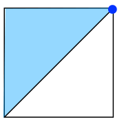
Finally, some readers may be surprised that we have focused so heavily on the study of global de Sitter space. In contrast, many treatments of de Sitter or inflation discuss only the inflating patch of de Sitter. Since the inflating patch has noncompact Cauchy surfaces, its Killing fields are not normally treated as generating gauge symmetries. In effect, one typically assumes (perhaps implicitly) that boundary conditions are imposed at the upper corner of the inflating patch (see figure 11.) such that the associated diffeomorphisms are non-trivial asymptotic symmetries rather than gauge. However, we are not aware of a complete technical specification and treatment of such boundary conditions and, perhaps as a result, many longstanding questions and confusions remain regarding the detailed relationship between analyses of global dS and analyses in the inflating patch. Nevertheless, it seems likely that, as discussed briefly in Higuchi:2011vw , the physics of global dS linearization stability constraints is directly related to large logarithms that arise when studying gravitational perturbation theory in the inflating patch; see, e.g., Seery_2010 and reference therein, Linde_2005 ; Giddings_2011 . It would thus be very interesting to better understand the implications of constructions described here for physics in the inflating patch and, in particular, to understand if (despite the seemingly different time-dependence involved) the above-mentioned large logarithms might be related to the fact that our perturbative gravity correlators become highly smeared versions of dS QFT correlators at late times.
Acknowledgements.
We thank Xi Dong, Gary Horowitz, and Geoff Penington for useful discussions. This research was supported by NSF grants PHY-2107939 and PHY-2408110, and by funds from the University of California. X.Y. was supported by the National Science Foundation Graduate Research Fellowship under Grant No. 2139319. Y.Z. was supported in part by the National Science Foundation under Grant No. NSF PHY-1748958, by a grant from the Simons Foundation (815727, LB), by Heising-Simons Foundation award-6950153, and by David and Lucile Packard Foundation Fellowship-2749255. Any opinion, findings, and conclusions or recommendations expressed in this material are those of the authors(s) and do not necessarily reflect the views of the National Science Foundation.Appendix A Group averaging and its extensions
This appendix addresses the finiteness and positivity properties of the group averaging inner product. We begin in section A.1 with a summary of results in the existing literature. We then propose a family (labeled by a single parameter ) of potential alternative inner products in section A.2. We use the uniqueness theorem of Giulini_1999 to argue that, if there is a value of such that this alternate inner product is well-defined on the space of states on which group-averaging converges absolutely, then the two inner products must coincide on , so that the alternate inner product is in fact an extension of the group-averaging inner product. The extended definition is manifestly positive semi-definite and, as discussed in section A.3, it assigns vanishing norm to all 1-particle states. One may also independently show that any allowed extension must assign vanishing norms to these states. For scalar fields with masses , this would thus suffice to show that the extended inner product is finite and positive semi-definite for seed states in a dense subspace of the space that is both orthogonal to the dS-invariant vacuum and orthogonal to all 2-particle states. Finally, the case of 2-particle states is discussed in section A.4, where we suggest that their divergent group-averaging norm is related to the fact that the corresponding classical solutions leave unbroken a non-compact subgroup of SO.
A.1 Summary of previous results
The case of linearized gravitons on dS4 turns out to be exactly solvable, and (2.2) was shown in Higuchi_1991_2 to be finite and positive semi-definite when is the space spanned by Fock basis-states with particles associated with the standard linearized graviton modes on global dS4. While it was not obviously finite for particle states, we will return to that case in section A.3 below.
For general massive free minimally-coupled scalar fields, the group averaging integral (2.2) was shown to be finite in Marolf:2010zp for standard Fock states that contain a sufficient number of particles. For scalar fields in the so-called principal series of SO representations (having where is the de Sitter length scale), this result holds for particles. The threshold particle number is higher for scalar fields than for the free gravitons studied in Higuchi_1991_2 because convergence is aided by adding angular momentum and because there are no gravitons with angular momentum quantum number (as defined in section 4) satisfying . The reader may think of this result as a generalization of Birkhoff’s theorem (which immediately excludes gravitons with ).
Larger numbers of particles are required for fields with smaller masses. The required number diverges as due to the fact that massless fields on dS have a zero mode, though sufficient excitations of this zero-mode also provide convergence; see Marolf:2008it for discussion of the dS1+1 case. For smaller numbers of particles the integral (2.2) fails to converge absolutely, though for the particle case this can be dealt with as described in section A.3 below.
A.2 An alternate definition?
An important part of justifying the group-averaging inner product (2.2) is that it satisfies a certain uniqueness result Giulini_1999 . We will now use this uniqueness to outline an argument that (2.2) is positive semi-definite when it converges absolutely. The argument involves the introduction of an alternate inner product which, if it is finite and non-zero on any state in the space on which group-averaging converges absolutely (and for which the group-averaging norm is non-zero), must agree with group-averaging on all of by the argument of Giulini_1999 . We in fact introduce a one-parameter family of potential alternate inner products in the expectation that there will be a value of this parameter which gives a finite no-zero result on . Unfortunately, however, the alternate inner products are difficult to compute. We thus leave detailed investigation of this expectation for future work.
Translating to the language of the current paper, the uniqueness theorem of Giulini_1999 shows that if is a space of states on which (2.2) converges absolutely, then there is an associated algebra of de Sitter-invariant linear operators defined by
| (A.1) |
for . Since the Haar measure is invariant under , these operators map to itself and also satisfy
| (A.2) |
for all . Here as usual we have defined . The theorem then shows that, up to an overall normalization, (2.2) is the unique product on that satisfies linearity with respect to the 2nd argument, the complex conjugation condition
| (A.3) |
the -representation condition111111The theorem of Giulini_1999 is stated in terms of so-called rigging maps which are analogues of (2.1). In that language, the main result is that the rigging map commutes with all . But the reality property of rigging maps together with (A.2) makes this equivalent to (A.4).
| (A.4) |
and with respect to which is a null vector for all and all .
As a result, if we can find another inner product satisfying the above properties on the same domain , it must be equivalent to (2.2) up to an overall normalization (though we must then check that this normalization constant is finite and non-zero). Let us therefore think of dSD as embedded in Minkowski space so that, choosing a standard set of inertial coordinates on that Minkowski space (with Minkowski metric ), we can write the generators of the de Sitter group as the generators of Lorentz transformations on Minkowski space and define the operators
| (A.5) |
For any real parameter we may then consider the inner product
| (A.6) |
where and where is the projection onto states with ; i.e., onto states that are invariant under the rotational subgroup SO SO. This inner product is written with round brackets to distinguish it from the other inner products used in this work. Expression (A.6) satisfies the complex conjugation condition (A.3) since
| (A.7) | |||||
| (A.8) |
Furthermore, since commutes with all rotations, and since (where is the normalized Haar measure on SO), we see that the factors , , and (or equivalently , , and ) all commute with each other. In the same way we see that if the integral in (A.6) converges, then we have
| (A.9) |
for all SO generators . For rotations this follows immediately from , while for boosts it follows from the fact that is the limit of projectors onto the part of the spectrum of in the range . Since is a positive-definite quadratic combination of the (see (A.5)), this implies that at finite it also restricts the spectrum of any to the interval . For , expressions like (A.9) then contain an extra factor of and thus vanish as . As a result, for and any we have
| (A.10) |
We can also show that the alternative inner product (A.6) satisfies the -representation condition (A.4). To do so, we simply note that commutes with all , and that it thus commutes with , , and . We may then use (A.2) to write
| (A.11) |
as desired.
As a result, if we can find a value of for which (A.6) is finite on the domain spanned by global dS Fock basis states which contain enough particles for group averaging to converge absolutely, and if (A.6) is finite non-zero for that and any choice of then, up to an overall normalization, for that and all the alternative inner product must agree with the group averaging inner product (2.2). Moreover, since can be expressed as a limit of spectral projections, the alternative inner product (A.6) is manifestly poistive-definite. Finding the above would then also establish positive semi-definiteness of group averaging on .
The existence of such an is certainly plausible, but the inner product (A.6) appears difficult to compute. We thus leave further investigation of this issue for future work.
A.3 One-particle states for free fields
In section A.2, we suggested that the inner product (A.6) (for some ) provides an alternative way of writing the group-averaging inner product (2.2) on the original domain . However, it can happen that expression (A.6) is well-defined for states where (2.2) is not. If the alternate and group-averaging inner products do in fact agree on for some , this would then suggest that (A.6) is well-defined on a domain that is strictly larger than the original domain . It would then be tempting to define the desired de Sitter invariant Hilbert space using (A.6) on the full domain . In this context, we could refer to (A.6) as an extended group-averaging inner product.
Of course, doing so immediately raises the question of the extent to which this supposed extension would be unique. We now will answer this question for the case of particle states for any free field. This is an interesting case since, when combined with the results reviewed in section A.1 and with the discussion of section A.4 below, it provides a rather complete picture of group-averaging for both 3+1 gravitons and free scalar fields with .
The alternate inner product (A.6) is well-defined for 1-particle states of any free field and, in fact, defines any 1-particle state to be a null state. To see this, note that the factor in (A.6) means that the only 1-particle state that could possibly have non-zero norm is the state associated with the zero angular-momentum mode of the field. Yang-Mills fields and gravitons have no such modes, so this completes the analysis for such cases. Similarly, for minimally-coupled massless scalars the zero angular-momentum mode is also a zero-frequency mode and so does not have particle excitations. While it would be interesting to return to states of that zero mode in the future (in order to extend the 1+1 analysis of Marolf:2008it ), this again completes the analysis of 1-particle states for such fields.
It thus remains only to consider fields with minimally-coupled masses . The 1-particle states of such fields are irreducible representations of SO with values of the quadratic Casimir . As a result, the rotationally-invariant one-particle state is an eigenstate of with eigenvalue . Thus must annihilate , so that is a null state under the inner product (A.6).
Furthermore, the above argument also shows these definitions to be unique. Indeed, let us consider a basis of one-particle states that are eigenstates of . If then, unless is proportional to the rotationally invariant state , the fact that is a sum of squares requires . We may thus write
| (A.12) |
But since must be a null state for all , the same must be true of . Thus (A.12) must be null as well. It then remains only to discuss the rotationally-invariant one-particle state . But it was shown above that this state is an eigenvector of with eigenvalue . It is thus of the form
| (A.13) |
The same argument used above then shows that must be null in .
The statement that one-particle states map to null states in is a direct analogue of the classical statement that any single particle in dS has at least one non-vanishing de Sitter charge. In particular, for free particles with mass , if one considers the static patch associated with the particle’s geodesic, then the corresponding static-patch energy takes the value . There are thus no classical single-particle states for which all de Sitter charges vanish.
A.4 The divergent group-averaging norm of 2-scalar-particle states
We now briefly address the case of 2-particle states of scalar fields. The asymptotic expansions of Marolf_2009 show that the group averaging norms of such states fail to converge absolutely and, in fact, that they in fact diverge linearly. This is a slower divergence than the exponential divergence one finds for the group-averaging norm of the de Sitter-invariant vacuum , but it is a divergence nonetheless. In fact, it is precisely the degree of divergence one would expect if such states left unbroken a 1-dimensional subgroup of SO generated by some boost transformation.
While the 2-particle states do not appear to leave such a group unbroken, the corresponding classical solutions do exhibit an unbroken such symmetry. Indeed, setting the de Sitter charges to zero forces a pair of classical particles to travel along antipodally-related geodesics (as in the particle approximation to the Schwarzschild-de Sitter solution). Such solutions clearly leave one boost symmetry intact; see figure 12. Some quantum version of this residual symmetry thus appears to be associated with the above divergence, though it would be useful to understand the relationship in more detail. In particular, following similar discussions in Marolf:1994ae , one might expect to be able to use an improved such understanding to argue that no well-defined de Sitter-invariant operator can cause such 2-particle states to mix with states having particles.
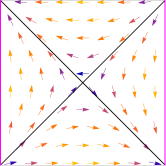
Appendix B Generator moments in for general dimensions
We now compute and analyze the coefficients in (4.13) associated with the expectation values of in the state for . Our goal is to extract useful expressions for these moments at leading order in large .
Let us start by computing the expectation value . On the states , the action of is
| (B.1) |
with
| (B.2) | ||||
| (B.3) |
Utilizing , this yields
| (B.4) |
As we will find with most of our other moments, a simple closed-form expression for this sum is not readily available. However, we are mostly interested in the asymptotic behavior at large , since in this limit the group averaging kernel will approximate a Gaussian with shrinking width. In particular, given our results in dS1+1, it is natural to take the ultrarelativistic limit . However, for now we will proceed with computing the remaining expectation values; we will then return later to the question of asymptotic behavior.
For , we find the result
| (B.5) |
Similarly, calculating gives
| (B.6) |
Finally, to find the expectation value of for , we use the Casimir equation
| (B.7) |
where we have used the notation . Since we have
| (B.8) |
we can easily compute .
We now return to the question of asymptotic behavior. For and , it is natural to assume that keeping only the leading terms in the summands will give the correct large behavior at leading order in . We will then check this assumption. The leading order behavior of the normalization constant is, using Stirling’s approximation, . And, in the limit and , we have
| (B.9) | ||||
| (B.10) |
(which have the same asymptotic behavior for or ). While this large limit will not hold for the terms in the sum where is small, we will shortly show that the terms where it fails do not contribute significantly in the limit of large . For convenience, we consider only , which differs from only by an overall sign. For , we have
| (B.11) |
where we have used Faulhaber’s formula for the sum: for the cases and . Similarly, for we find
| (B.12) |
Finally, the Casimir equation (B.7) yields
| (B.13) |
We may now verify that the above guess indeed gives the correct large behavior of the desired moments (despite the fact that we used Equations (B.9) and (B.10) in regimes where they were not fully applicable). For our summands , we have
| (B.14) |
since is increasing with . In particular, for we find
| (B.15) |
The lower bound evaluates to
| (B.16) |
We can see that the upper bound will also evaluate to . Thus, we must have
| (B.17) |
The same argument holds for , proving we have the correct asymptotic behavior of our sums.
We will also need to find for and . The symmetry of requires all to be equal for . Additionally, all with (or ) must be equal, while all others must vanish. We thus find,
| (B.18) | ||||
| (B.19) | ||||
| (B.20) |
References
- (1) B. S. DeWitt, The quantization of geometry, in Gravitation: An introduction to current research, L. Witten, ed., (New York, NY), Wiley, 1962.
- (2) B. S. DeWitt, Quantum Theory of Gravity. 1. The Canonical Theory, Phys. Rev. 160 (1967) 1113.
- (3) T. Banks, T C P, Quantum Gravity, the Cosmological Constant and All That…, Nucl. Phys. B 249 (1985) 332.
- (4) J. B. Hartle, Prediction in Quantum Cosmology, NATO Sci. Ser. B 156 (1987) 329.
- (5) C. Rovelli, Quantum mechanics without time: a model, Phys. Rev. D 42 (1990) 2638.
- (6) C. Rovelli, Quantum reference systems, Class. Quant. Grav. 8 (1991) 317.
- (7) C. Kiefer, The Semiclassical approximation to quantum gravity, Lect. Notes Phys. 434 (1994) 170 [gr-qc/9312015].
- (8) D. Marolf, Almost ideal clocks in quantum cosmology: A Brief derivation of time, Class. Quant. Grav. 12 (1995) 2469 [gr-qc/9412016].
- (9) S. B. Giddings, D. Marolf and J. B. Hartle, Observables in effective gravity, Phys. Rev. D 74 (2006) 064018 [hep-th/0512200].
- (10) D. Marolf, Comments on Microcausality, Chaos, and Gravitational Observables, Class. Quant. Grav. 32 (2015) 245003 [1508.00939].
- (11) E. Witten, Gravity and the crossed product, JHEP 10 (2022) 008 [2112.12828].
- (12) V. Chandrasekaran, R. Longo, G. Penington and E. Witten, An algebra of observables for de Sitter space, JHEP 02 (2023) 082 [2206.10780].
- (13) V. Chandrasekaran, G. Penington and E. Witten, Large N algebras and generalized entropy, JHEP 04 (2023) 009 [2209.10454].
- (14) K. Jensen, J. Sorce and A. J. Speranza, Generalized entropy for general subregions in quantum gravity, JHEP 12 (2023) 020 [2306.01837].
- (15) G. Penington and E. Witten, Algebras and States in JT Gravity, 2301.07257.
- (16) J. Kudler-Flam, S. Leutheusser and G. Satishchandran, Algebraic Observational Cosmology, 2406.01669.
- (17) C.-H. Chen and G. Penington, A clock is just a way to tell the time: gravitational algebras in cosmological spacetimes, 2406.02116.
- (18) S. B. Giddings and D. Marolf, A global picture of quantum de sitter space, Physical Review D 76 (2007) [0705.1178].
- (19) S. Kachru, R. Kallosh, A. D. Linde and S. P. Trivedi, De Sitter vacua in string theory, Phys. Rev. D 68 (2003) 046005 [hep-th/0301240].
- (20) L. McAllister, J. Moritz, R. Nally and A. Schachner, Candidate de Sitter Vacua, 2406.13751.
- (21) D. Marolf, Quantum observables and recollapsing dynamics, Class. Quant. Grav. 12 (1995) 1199 [gr-qc/9404053].
- (22) D. Marolf, Observables and a Hilbert space for Bianchi IX, Class. Quant. Grav. 12 (1995) 1441 [gr-qc/9409049].
- (23) Y. Aharonov and L. Susskind, Charge Superselection Rule, Phys. Rev. 155 (1967) 1428.
- (24) Y. Aharonov and T. Kaufherr, Quantum frames of reference, Phys. Rev. D 30 (1984) 368.
- (25) L. Loveridge, T. Miyadera and P. Busch, Symmetry, Reference Frames, and Relational Quantities in Quantum Mechanics, Found. Phys. 48 (2018) 135 [1703.10434].
- (26) P. A. Hoehn, A. R. H. Smith and M. P. E. Lock, Trinity of relational quantum dynamics, Phys. Rev. D 104 (2021) 066001 [1912.00033].
- (27) C. J. Fewster, D. W. Janssen, L. D. Loveridge, K. Rejzner and J. Waldron, Quantum reference frames, measurement schemes and the type of local algebras in quantum field theory, 2403.11973.
- (28) J. De Vuyst, S. Eccles, P. A. Hoehn and J. Kirklin, Gravitational entropy is observer-dependent, 2405.00114.
- (29) A. Higuchi, Quantum linearization instabilities of de Sitter space-time. 1, Class. Quant. Grav. 8 (1991) 1961.
- (30) A. Higuchi, Quantum linearization instabilities of de Sitter space-time. 2, Class. Quant. Grav. 8 (1991) 1983.
- (31) S. Deser and D. Brill, Instability of Closed Spaces in General Relativity, Commun. Math. Phys. 32 (1973) 291.
- (32) V. Moncrief, Space-Time Symmetries and Linearization Stability of the Einstein Equations. 1., J. Math. Phys. 16 (1975) 493.
- (33) V. Moncrief, Space-Time Symmetries and Linearization Stability of the Einstein Equations. 2., J. Math. Phys. 17 (1976) 1893.
- (34) J. Arms, Linearization stability of the Einstein–Maxwell system, J. Math. Phys. 18 (1977) 830.
- (35) J. M. Arms, Linearization Stability of Gravitational and Gauge Fields, J. Math. Phys. 20 (1979) 443.
- (36) D. Marolf, The Spectral analysis inner product for quantum gravity, in 7th Marcel Grossmann Meeting on General Relativity (MG 7), pp. 851–853, 9, 1994, gr-qc/9409036.
- (37) A. Ashtekar, J. Lewandowski, D. Marolf, J. Mourao and T. Thiemann, Quantization of diffeomorphism invariant theories of connections with local degrees of freedom, J. Math. Phys. 36 (1995) 6456 [gr-qc/9504018].
- (38) D. Giulini and D. Marolf, On the generality of refined algebraic quantization, Class. Quant. Grav. 16 (1999) 2479 [gr-qc/9812024].
- (39) D. Marolf, Group averaging and refined algebraic quantization: Where are we now?, in 9th Marcel Grossmann Meeting on Recent Developments in Theoretical and Experimental General Relativity, Gravitation and Relativistic Field Theories (MG 9), 7, 2000, gr-qc/0011112.
- (40) T. Chakraborty, J. Chakravarty, V. Godet, P. Paul and S. Raju, Holography of information in de Sitter space, JHEP 12 (2023) 120 [2303.16316].
- (41) D. Marolf, Path integrals and instantons in quantum gravity: Minisuperspace models, Phys. Rev. D 53 (1996) 6979 [gr-qc/9602019].
- (42) R. F. Streater and A. S. Wightman, PCT, spin and statistics, and all that. 1989.
- (43) N. Y. Vilenken and A. U. Klimyk, Representations of Lie Groups and Special Functions, vol. 1-3. Dordrecht: Kluwer Acad. Publ, 1991-1993.
- (44) M. K. F. Wong, Unitary representations of so(n,1), J. Math. Phys. 15 (1974) 25.
- (45) Z. Sun, A note on the representations of , 2111.04591.
- (46) D. Marolf and I. A. Morrison, Group averaging for de sitter free fields, Classical and Quantum Gravity 26 (2009) 235003 [0810.5163].
- (47) S. Gao and R. M. Wald, Theorems on gravitational time delay and related issues, Class. Quant. Grav. 17 (2000) 4999 [gr-qc/0007021].
- (48) P. C. Aichelburg and R. U. Sexl, On the Gravitational field of a massless particle, Gen. Rel. Grav. 2 (1971) 303.
- (49) J. J. Halliwell and J. B. Hartle, Wave functions constructed from an invariant sum over histories satisfy constraints, Phys. Rev. D 43 (1991) 1170.
- (50) M. P. Reisenberger and C. Rovelli, ’Sum over surfaces’ form of loop quantum gravity, Phys. Rev. D 56 (1997) 3490 [gr-qc/9612035].
- (51) D. Marolf and H. Maxfield, Transcending the ensemble: baby universes, spacetime wormholes, and the order and disorder of black hole information, JHEP 08 (2020) 044 [2002.08950].
- (52) D. Giulini and D. Marolf, A uniqueness theorem for constraint quantization, Classical and Quantum Gravity 16 (1999) 2489–2505 [9902045].
- (53) A. Higuchi, D. Marolf and I. A. Morrison, de Sitter invariance of the dS graviton vacuum, Class. Quant. Grav. 28 (2011) 245012 [1107.2712].
- (54) D. Seery, Infrared effects in inflationary correlation functions, Classical and Quantum Gravity 27 (2010) 124005 [1005.1649].
- (55) A. Linde, Particle physics and inflationary cosmology, 2005.
- (56) S. B. Giddings and M. S. Sloth, Cosmological observables, infrared growth of fluctuations, and scale-dependent anisotropies, Physical Review D 84 (2011) [1104.0002].
- (57) D. Marolf and I. A. Morrison, The IR stability of de Sitter: Loop corrections to scalar propagators, Phys. Rev. D 82 (2010) 105032 [1006.0035].
- (58) D. Marolf and I. A. Morrison, Group Averaging of massless scalar fields in 1+1 de Sitter, Class. Quant. Grav. 26 (2009) 035001 [0808.2174].