A Unified Multi-Wavelength Data Analysis Workflow with gammapy

Abstract

Context. The Flat Spectrum Radio Quasar OP 313 entered an enhanced activity phase in November 2023 and has undergone multiple flares since then which have motivated the organisation of several large multi-wavelength campaigns, including two deep observations from the hard X-ray telescope NuSTAR. The broadband emission from OP 313 during these two observations is investigated under a new unified analysis framework, with data spanning from optical to $\gamma$ rays.

Aims. Traditional methods for analyzing blazar emissions often rely on proprietary software tailored to specific instruments, making it challenging to integrate and interpret data from multi-wavelength campaigns comprehensively. This study demonstrates the feasibility of utilizing gammapy, an open-source Python package, and common data formats originally developed for $\gamma$-ray instrumentation, to perform a consistent multi-instrument analysis. This enables a forward folding approach that fully incorporates source observations, detector responses, and various instrumental and astrophysical backgrounds. The methodology is applied as an example to recent data collected from the distant quasar OP 313.

Methods. We present a comprehensive data reconstruction and analysis for instruments including the Liverpool Telescope’s IO:O detector, Swift-UVOT, Swift-XRT, NuSTAR, and Fermi-LAT. The resulting spectral analysis is validated against the native tools for each instrument. Additionally, a multi-wavelength phenomenological model of the source emission, encompassing optical to $\gamma$-ray bands, is developed, incorporating absorption components across different energy regimes.

Results. We introduce and validate a new unified framework for multi-wavelength forward folding data analysis based on gammapy and open data formats, demonstrating its application to spectral data from the quasar OP 313. This approach provides a more statistically correct treatment of the data than fitting a collection of flux points extracted from the different instruments. This study is the first to use a common event data format and analysis tool covering 11 orders of magnitude in energy, from approximately 1 eV to 100 GeV. The high-level event data, instrument response functions, and models are provided in a gammapy-compatible format, ensuring accessibility and reproducibility of scientific results. A brief discussion on the origin of OP 313’s broadband emission is also included.

1 Introduction

Active Galactic Nuclei (AGNs), in particular those with large-scale jets of ultra-relativistic particles, are the predominant extragalactic sources of $\gamma$-ray photons. Their non-thermal emission extends over the entire electromagnetic spectrum, from radio to $\gamma$ rays, yet the driving physical mechanism that explains the radiation in each band is different. At low energies, from radio to optical (in some cases up to X-rays), the emission is often assumed to be mainly due to synchrotron radiation from relativistic electrons (Konigl 1981). At higher energies, the situation is less clear and diverse mechanisms are assumed to explain the emission, from inverse Compton of the same electrons with the synchrotron radiation (synchrotron-self-Compton or SSC, see Maraschi et al. 1992) or with external thermal photons from the AGN structure (external Compton or EC, e.g. Dermer & Schlickeiser 1993), to various hadronic processes: proton-synchrotron, proton-proton (see e.g. Aharonian 2002).

Flat Spectrum Radio Quasars (FSRQs) are a subclass of AGNs characterized by jets closely aligned with the line of sight and strong thermal radiation components from the AGN accretion disk in the optical-UV band. This radiation is partially reprocessed into thermal emission by the dusty torus in the infrared and into Doppler-broadened emission lines in the broad line region (BLR). These thermal radiation fields are significant targets for Compton (up)scattering, making FSRQs often very luminous in the $\gamma$-ray band, especially during flares. This process is a major cooling mechanism for the accelerated electrons, as the electrons lose energy by scattering photons to higher energies. The high luminosity and close jet alignment makes FSRQs detectable at greater distances compared to BL Lac objects, which lack strong thermal components.

However, detecting very-high-energy (VHE; E $>$ 100 GeV) $\gamma$-ray emission from AGNs — especially for those found at high redshifts — is challenging due to attenuation by the extragalactic background light (EBL, e.g. Domínguez et al. 2011; Saldana-Lopez et al. 2021), which absorbs $\gamma$-rays from distant sources and is an irreducible background that encodes important information about the star formation history in the Universe. The induced absorption produces an energy-dependent imprint on the blazar spectrum, reducing significantly the observable $\gamma$-ray flux in the VHE band. At the same time, it provides an opportunity to constrain the density of the EBL indirectly, provided that we can infer the intrinsic spectrum of the source. For sources at redshift $z\sim 1$ and sub-TeV photons, the most relevant part of the spectrum of the EBL is the so-called Cosmic Optical Background component.

OP 313 is a FSRQ at a redshift of $z=0.997$ (Schneider et al. 2010), which has experienced several flaring states over the past 15 years, as evidenced by continuous monitoring with the Fermi-LAT $\gamma$-ray space telescope. In November 2023, OP 313 entered a multi-month high state, with daily energy flux often exceeding $\mathrm{F(>\,100\,MeV)\gtrsim 10^{-10}\,erg\,cm^{-2}\,s^{-1}}$ in the Fermi light curve repository (Abdollahi et al. 2023), representing the brightest flare for this source since Fermi’s launch in 2008, more than two orders of magnitude over the quiescent state flux. Around February 29th, the source reached a record high of $(2.96\pm 0.57)\times 10^{-9}\mathrm{erg\,cm^{-2}\,s^{-1}}$. At $z=0.997$, this flaring episode makes OP 313 one of the most luminous AGNs ever recorded in $\gamma$ rays. Follow-up observations with the Large-Sized Telescope prototype (LST-1) Cherenkov telescope began in December 2023 and led to the first detection of this source at VHEs, making OP 313 the most distant AGN ever detected by a Cherenkov telescope (Cortina & CTAO LST Collaboration 2023). Since then, the CTAO LST Collaboration has led a very intense multi-wavelength monitoring campaign of the source, which have driven the development of new analysis techniques like the one presented in this work. The detection of such a bright and distant source, coupled with the methodologies described herein, offers a unique opportunity to constrain the dynamic emission of the source and provides a good benchmarking tool to test EBL models using physically-motivated intrinsic emission models.

In this work, we aim to validate a new analysis and data management workflow based on the standard format proposed by the Data formats for $\gamma$-ray astronomy (Nigro et al. 2021) and the open-source tool gammapy (Donath et al. 2023), and provide a working prototype data archive for the source, retaining full instrument response metadata for reproducibility in future analyses and interpretation of these observations. This manuscript focuses on demonstrating and validating a new methodology for multi-wavelength analysis. For this demonstration we combined datasets from a small coordinated multi-wavelength follow-up campaign on OP 313 developed on March 4th 2024 (MJD60373) and March 15th (MJD60384), utilizing public data from Swift-UVOT, Swift-XRT, NuSTAR, and Fermi-LAT, and data from Liverpool IO:O in the optical regime. The resulting data products, in standard OGIP/GADF formats compatible with gammapy, are readily available in GitHub and described in more details in Appendix A. We leave the integration of this dataset with a larger campaign, including proprietary VHE $\gamma$-ray data from LST and MAGIC, as well as additional optical, infrared, and radio results, for a separate work coordinated by the CTAO LST Collaboration. To keep the main body of the manuscript as focussed as possible, we will refer always to data and results from the first observing night on March 4th, 2024 (MJD60373), and comment briefly on the results of the application of the analysis framework to the second night on March 15th, 2024 (MJD60384) in Appendix E.

Our proposed method involves a forward modeling approach within a unified framework for all multi-wavelength datasets, covering optical (z band) to HE $\gamma$-rays, spanning nearly twelve orders of magnitude in energy. The mathematical representation of this method is as follows:

$$\begin{split}N(E,X)=\sum_{sources}\mathcal{R}&(E,E_{\rm true},X)\ast\mathcal{P}(E_{\rm true},X,X_{true})\\ \ast&\left[\mathcal{E}(E_{\rm true},X_{true})\times\phi(E_{\rm true})\right],\end{split}$$ (1)

where the number of expected excess event density $N(E,X)$ (in space and energy) is given as a function of the sum over a number of finite emitters of the differential spectrum $\phi(E_{\rm true})$ of each source times the exposure at its location, convoluted with the PSF $\mathcal{P}(E_{\rm true},X,X_{true})$, which informs about the actual distribution of the measured counts given a location in the detector/sky, possibly as a function of energy, and a redistribution or migration matrix $\mathcal{R}(E,E_{\rm true},X)$ which provides the relation between the theoretical energy and the measured energy of the event, as a function of location in the detector/sky.

The manuscript is structured as follows: Section 2 details the motivation behind developing a new method for analyzing and archiving high-level data across multiple bands. Section 3 describes the different instruments and procedures used to build the datasets and Instrument Response Functions (IRFs). Section 4 presents the validation of the data formats and analysis methods, along with a phenomenological model of the emission of the source. The discussion of limitations, possible extensions, and future work is included in Section 5, and the main results are summarized in Section 6. Wherever applicable, we use a flat $\mathrm{\Lambda}$CDM cosmology, with $\mathrm{H_{0}=70\,km\,s^{-1}\,Mpc^{-1}}$, $\mathrm{\Omega_{M}}=0.3$, and $\mathrm{T_{CMB,0}=2.725\ K}$.

2 Motivation

Accurately modeling the spectral energy distribution (SED) of flaring AGNs across multiple wavelengths is a complex task due to the inherent challenges in handling diverse data types and formats. The traditional approach isolates each instrument or energy regime to ‘reconstruct’ or estimate flux points and upper limits (ULs), followed by a reinterpretation of the same points using physically motivated models (see e.g. Ahnen et al. 2015; MAGIC Collaboration et al. 2023). However, this method has several limitations.

Firstly, storing flux points in tables or plots often results in significant information loss. This approach typically fails to account for the energy resolution of the instruments if no unfolding (Schmitt 2017) is performed, a process that is inherently ill-posed. Consequently, the flux points may become correlated. Additionally, errors are commonly treated as Gaussian, which is inappropriate for instruments operating in low-count regimes where Poissonian statistics are more suitable (see e.g. Yamada et al. 2019). ULs are frequently represented as single values at specific confidence levels, resulting in the loss of information contained in the underlying probability distributions. This practice can lead to biased interpretations, especially when statistical fluctuations, ULs and non-detections are ignored (e.g. Essey & Kusenko 2014).

Moreover, current methods fall short in handling multiplicative models in SED flux points, such as correcting for hydrogen column density ($N_{H}$) in X-ray data, extinction in optical/UV or EBL absorption in the $\gamma$-ray regime. Typically, these corrections are applied to the reconstructed flux points, which can hinder accurate statistical correction for absorption components in the SED, particularly if the correction is applied differently for each dataset (this is sometimes the case for optical instruments).

Recent advancements have explored moving away from flux points towards forward-folding techniques, which have demonstrated promising results in characterizing the EBL (Acciari et al. 2019) using VHE data. This forward-folding approach offers a more comprehensive statistical analysis of multi-wavelength datasets, addressing many shortcomings of traditional flux-point methods. Although forward-folding is inherently model-dependent, it provides greater stability compared to unfolding methods while solving the same underlying problem. By incorporating forward modeling, emission and absorption models can be seamlessly integrated into the analysis, enabling better handling of uncertainties in parameters such as hydrogen column density and EBL. In this work we address one of the main drawbacks of the forward-folding method, which is how to distribute the actual data together with a consistent description of the instrument that allows to interpret it without the need to install the software for each instrument.

Our immediate goal is therefore to integrate high-level data from various photon-counting experiments into a unified analysis framework. To facilitate this, we propose using the standardized format for high-level data products, which ensures easier distribution of the data and instrument description, as well as reproducibility of the results. gammapy, an open-source Python package based on the popular libraries numpy (Harris et al. 2020) and astropy (Astropy Collaboration et al. 2013, 2018, 2022), is particularly well-suited for this task. As the official science tool for the Cherenkov Telescope Array Observatory (CTAO), gammapy is actively developed and compatible with both OGIP (X-ray) and GADF ($\gamma$-ray) data formats. This makes it an ideal choice for our analysis, enabling the joint analysis of different types of datasets, whether one-dimensional (1D) if only a distribution of counts as a function of energy is stored, or three-dimensional (3D) where data cubes of three dimensions (two spatial coordinates and one energy coordinate) are available. Finally, we show that even in the case of single-channel photometric datasets the proposed format is well suited to describe the data.

Furthermore, gammapy allows the incorporation of physically motivated models through external emission libraries — including synchrotron, inverse Compton, absorption components such as EBL absorption — or even extend it with models from the X-ray library sherpa (Freeman et al. 2001; Doe et al. 2007) to add hydrogen absorption, and interstellar extinction. Public radiation codes like agnpy (Nigro et al. 2022), jetset (Tramacere et al. 2009, 2011; Tramacere 2020), and naima (Zabalza 2015) offer a more accurate representation of underlying physical processes compared to traditional functional or empirical models available in standard X-ray analysis packages like xspec (Arnaud 1996) and sherpa (Freeman et al. 2001; Doe et al. 2007). This capability allows for a more accurate and statistically robust comparison of different models.

The proposed workflow can be compared with the Multi-Mission Maximum Likelihood framework (3ML, Vianello et al. 2015; Burgess et al. 2021), a versatile tool designed to facilitate multi-wavelength analysis by integrating various software packages tailored for different types of observational data (see e.g. Albert et al. 2023; Klinger et al. 2024). However, 3ML requires a complex setup involving the installation and configuration of multiple software tools within a common environment to ‘export’ the likelihood functionality for each instrument. This integration involves ensuring seamless communication between tools such as xspec for X-ray data, Fermipy or gammapy for $\gamma$-ray analysis, and other domain-specific software for optical photometric data. In contrast, while our method requires the preliminary construction of IRFs, it provides a unified data format and analysis workflow that supports the integration of multi-wavelength data without the need for multiple software environments. By design, the proposed methodology simplifies the analysis setup, enhances portability, and improves reproducibility compared to the arguably more cumbersome process required by 3ML.

In the following sections, we will detail the components of our methodology, and describe the dataset and IRF generation for the case of study of the flaring blazar OP 313. Our proposed framework aims to enhance the accuracy of SED modeling and streamline the analysis process across diverse astrophysical datasets and improve the reproducibility of the results. This work focuses on the technical implementation and presents validation tests in comparison to the standard analysis tools and methods used for each instrument.

3 Dataset construction

3.1 Fermi-LAT data reduction

The Large Area Telescope (LAT, Atwood et al. 2009) onboard the Fermi satellite is a space-based, pair-conversion telescope surveying the sky in the high-energy $\gamma$-ray band ($\lesssim 100\,$MeV to $\gtrsim 100\,$GeV). It covers $20\%$ of the sky instantaneously and surveys the entire sky approximately every $\sim 3$ hours, making it an excellent instrument for studying transient phenomena, including AGN flares.

3.1.1 Data reduction

We collected Fermi-LAT Pass 8 SOURCE class events with energies larger than $100\,$MeV within a region of interest (ROI) of $15\,$deg radius around the OP 313 position from October 1, 2023, to April 1, 2024 (183 days). Night-by-night binned analyses (centered at 00:00 UTC were performed with the Fermi Science Tools (Fermi Science Support Development Team 2019), using enrico (Sanchez & Deil 2015) as a high-level wrapper to manage the individual jobs. We utilized the latest available version of LAT’s IRFs (P8R3_SOURCE_V3) and applied a conservative zenith cut of $90\,$deg to avoid Earth’s limb contamination and a DATA_QUAL==1 && LAT_CONFIG==1 filter to ensure that only good quality events were analyzed, following the recommendations in Cicerone.

The sky model for the analysis was generated using the Fermi-LAT 14-Year Point Source Catalog (4FGL-DR4 Abdollahi et al. 2022; Ballet et al. 2023), incorporating sources within a $20\,$deg radius around OP 313. Spectral parameters for weak sources ($<10\,\sigma$ significance) and distant sources ($>5\,$deg) were fixed, except for normalizations. For OP 313, and because we only integrate $24\,$h per analysis, we adopted a simple power-law (PWL) spectral model, including the EBL absorption model from Domínguez et al. (2011). Positions and extensions of all sources from the 4FGL-DR4 were fixed, leaving only the spectral parameters of OP 313 (normalization and spectral index) and the normalization of the isotropic background component as free parameters.

3.1.2 Long-term analysis of the high-energy flare

In addition to focusing on two specific nights with comprehensive multi-wavelength coverage, we examined the broader activity of OP 313 to contextualize its emission during these nights within a longer-term flare that has persisted for several months in 2023-2024. Figure 1 shows the evolution of the nightly flux above $100\,$MeV for OP 313, with 24-hour bins centered at midnight UTC. It also depicts the evolution of the spectral index in the Fermi-LAT band and its correlation with the estimated flux, hinting that during high emission states, the spectrum of OP 313 becomes harder, with an index in the LAT band smaller than $\sim 2$. From Figure 1, we observe that the source entered an intermediate $\gamma$-ray activity plateau phase following a very strong flare at the end of February.

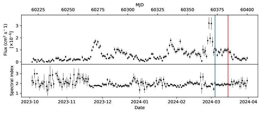
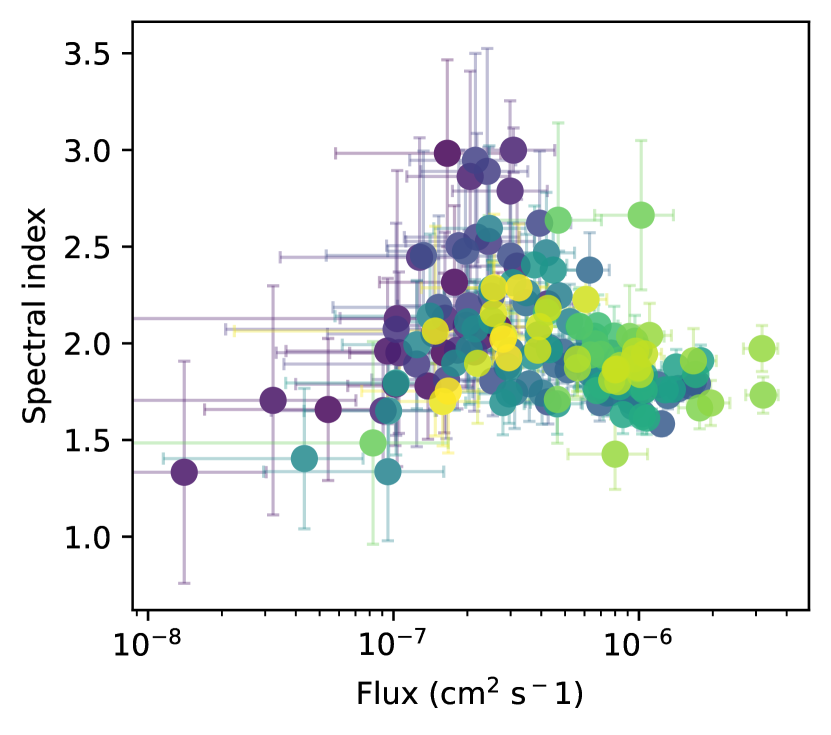
Figure 1: Left: Fermi-LAT light curve (1-day binning) of OP 313 above 100 MeV during the major 2023-2024 flare episode, for integral flux and spectral index. Blue and red bars mark the two nights with NuSTAR observations that are the focus of this study. Right: Spectral index as a function of the integral flux for each night over six months of LAT data. The density of points is color-coded, with yellow points showing larger number density of nights and purple-blue tones indicating more isolated bins.

3.1.3 Dataset and IRFs

For Fermi-LAT, the dataset is managed as a 3D MapDataset in gammapy, which includes spatial (two coordinates) and energy (one coordinate) dimensions. Figures 2 shows 2D and 1D projected representations of the different parts giving shape to the Dataset. From first row, left, to second row, right, the following information is shown:

1. Integral Counts Map: a 2D representation of the underlying ‘counts cube’ summed over the entire energy range and smoothed with a Gaussian kernel of $0.2$ deg to enhance visibility of sources.

2. Initial Model Map convolved with the IRFs to produce the predicted counts (npred map) and again integrated over the entire energy range just for visualization purposes. The original, 3D version, of this Model is fit to the data (‘counts cube’) by gammapy.

3. Containment Radius: 1D representation of the PSF corresponding to $68\%$ and $95\%$ of the events contained as a function of energy, indicating the spatial resolution of the LAT. As opposed to the native analysis, Fermitools, our conversion to gammapy format assumes a non-varying PSF. For a bright point-like source analysis in a $20\,$deg region size, we estimate the impact of not modelling the PSF correctly at the edges to be negligible.

4. Energy Dispersion: Shows the distribution of reconstructed energies versus true energies, providing information on how accurately the instrument measures the energy of $\gamma$-ray events and possible energy biases (mostly present at the lowest energies, $E\lesssim 100\,$MeV).

5. Exposure Map: 2D projection of the exposure (effective area multiplied by livetime) at $30.6\,$GeV, illustrating the spatial variation in exposure across the FoV.

6. Exposure at the FoV Center: 1D projection of the exposure as a function of true energy at the center of the field of view, showing the energy dependence of the LAT’s sensitivity.

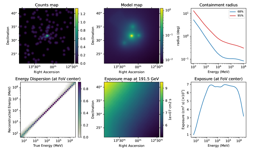
Figure 2: Fermi-LAT dataset description for the first selected night. From top left to bottom right: (a) Integral counts map, smoothed with a Gaussian kernel of $0.2$ deg. (b) Initial model map, convolved with the IRFs (npred map). (c) $68\%$ and $95\%$ containment radius as a function of energy. (d) Energy dispersion (reconstructed energy as a function of true energy). (e) Exposure map at $191.5\,$GeV. (f) Exposure at the FoV center as a function of true energy.

3.2 NuSTAR data reduction

The Nuclear Spectroscopic Telescope Array (NuSTAR, Harrison et al. 2013) is a focusing high-energy X-ray telescope operating in the 3 to 79 keV energy range. NuSTAR is a telescope array consisting on two twin modules (NuSTAR A and NuSTAR B), each made of four Cadmium-Zinc-Tellurium detectors.

The standard data products provided to the observer are similar to other X-ray space telescopes and consist of an event list where the most important columns are the reconstructed position, energy and time of arrival of each detected X-ray photon.

The typical data reduction procedure used in X-ray astronomy is to define a spatial region for spectral extraction and an OFF region to estimate the spectral background. The data reduction and first stages of the analysis were performed with nustardas v2.1.2. The data were obtained from the quick-look area for observation IDs 91002609002 (night of March 4th, 2024) and 91002609004 (night of March 15th, 2024). We ran nupipeline to process the data through Stage 1 (data calibration) and Stage 2 (data screening) for each of the nights and each of the telescope modules.

In a second step, we ran nuproducts (Stage 3) over the Level 2 event files to extract the integrated bandpass images ($3-79\,$keV), the source spectrum and light curves. Each NuSTAR module and sector has slightly different properties, therefore the background extraction regions were optimized for each module in shape and location to maximize background statistics, but keeping it within the limits of the same sector in which the source is located (see Fig. 3). From this point, we focus only on the spectral analysis of the Level 3 data produced by nuproducts, consisting of: (i) PHA files (energy spectra) for the source and background; (ii) ARF file (Ancilliary Response File), which contains the effective area; and (iii) RMF file (Response or Redistribution Matrix File), containing the energy migration matrix, a 2D-array that gives the probabilities of assigning the photon to a given PHA channel for each input photon energy.

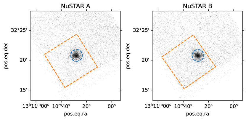
Figure 3: NuSTAR A/B counts map for the first observation night, together with the signal extraction region (blue dashed circle) and background extraction region (orange dashed box minus the signal extraction circle).

3.2.1 Background model

Two analyses of the spectral data were considered, each with different background assumptions. The first analysis uses the ON-OFF method with W-statistics (W-statistics, wstat, or Poisson data with a Poisson background). In this approach, the background is estimated measuring the number of events in the OFF region (see Fig.3), assuming that it is the same as in the source region once correcting for the region size differences. This method is straightforward but can not account for any spatial variation of the background (e.g. instrumental lines). In addition, it is statistically limited, as the W-statistic estimator can produce inaccurate results in low-count regimes, particularly if the background reaches zero counts in a given energy bin. To mitigate these issues, we re-binned the data into coarser energy bins to increase the statistics per bin.

The second approach involves using a background model for NuSTAR data. We employed the Cosmic X-ray Background (CXB) simulation tool nuskybgd (Wik et al. 2014) to estimate the background (using C-statistics, cstat, or Poisson data with a background model). Compared to a directly measured background via the OFF background method, the predicted background from nuskybgd effectively addresses issues related to very low statistics at high energies. At the cost of the complexity added by nuskybgd, this approach retains better spectral resolution while fully utilizing the energy range of NuSTAR, and accounts for the spatial variation of instrumental background. A detailed comparison of the impact of the choice of the background method is presented in Appendix B.

3.2.2 Dataset and IRFs

An overall view of the datasets for the NuSTAR A module on the first of the two available nights, with both the Poisson measured background (gammapy’s SpectrumDatasetOnOff object) and the one with nuskybgd background model (gammapy’s SpectrumDataset object), is shown in Fig. 4.

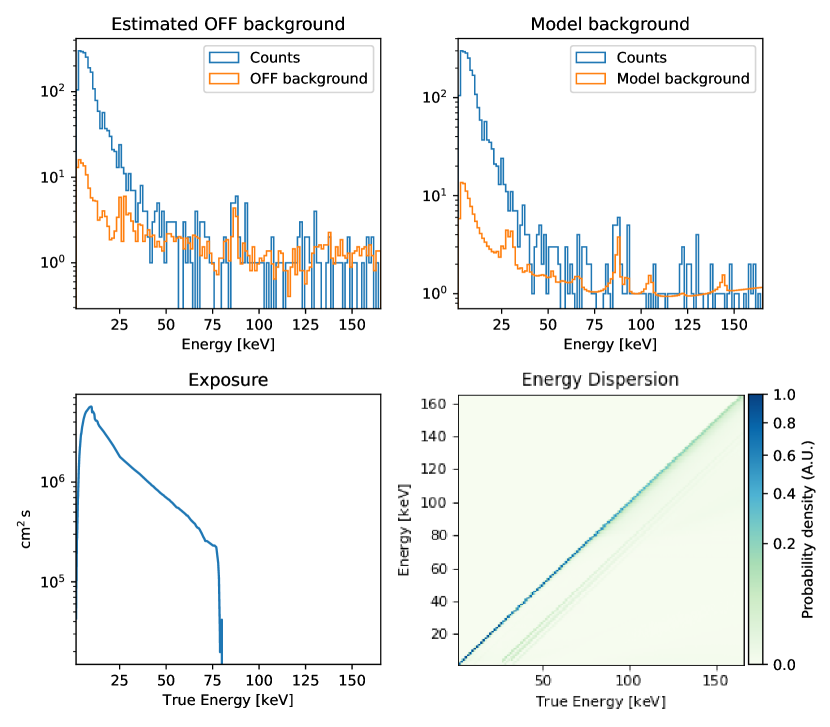
Figure 4: gammapy dataset representation of NuSTAR A for night 1 is shown here. NuSTAR B for this observation and NuSTAR A/B for night 2 are similar. From top left to bottom right: (a) Estimated distribution of background events from the OFF rectangular region of Figure 3 and ON event distribution from the signal extraction region. (b) Estimated distribution of background events from nuskybgd. ON event distribution identical to the previous case. (c) NuSTAR A exposure (effective area $\times$ livetime) as a function of true energy. (d) NuSTAR A energy dispersion matrix.

3.3 Swift-XRT data reduction

The X-Ray Telescope (XRT, Burrows et al. 2004) onboard the Swift satellite is an X-ray CCD imaging spectrometer designed to measure the position, spectrum, and brightness of astronomical objects in the range of $0.2$ to $\sim 10\,$ keV, with a dynamic range spanning more than seven orders of magnitude in flux. XRT has an effective area of approximately $135\,\mathrm{cm^{2}}$ at 1.5 keV and a detection sensitivity of $2\times 10^{-14}\,\mathrm{erg\,cm^{-2}\,s^{-1}}$ in $10\,$ ks of observing time.

The FoV is $23.6\times 23.6$ arcmin, with an angular resolution of $18$ arcsec (Half-Energy Width, HEW). XRT operates in two readout modes: Windowed Timing (WT) and Photon Counting (PC). The WT mode bins 10 rows into a single row, focusing on the central 200 columns to improve time resolution to $1.7\,$ ms (ideal for bright sources), while the PC mode retains full imaging and spectroscopic capabilities but with a slower time resolution of $2.5$ s and is limited by pileup effects at high count rates ($\gtrsim 0.6\,$ c/s, Vaughan et al. 2006). OP 313 is a relatively weak X-ray source with a modest count rate of $\lesssim 0.2\,$ c/s, well within the capabilities of XRT in PC mode; therefore, this work focuses exclusively on this mode.

Swift-XRT data for OP 313 were downloaded from the UK Swift Science Data Centre. Of all available data from the telescope, this work focuses on data collected during the nights of March 4th, 2024 and March 15th, 2024, with Swift observation IDs 00036384074 ($2.96\,$ks) and 00089816002 ($3.16\,$ks), respectively. We used Heasoft 6.32.1 and xrtdas v3.7.0 for data reduction. Spectra were extracted and saved using ximage for fixed source and background regions (see Fig. 5) in two separate PHA files. The corresponding Response Matrix File (RMF) file was downloaded from HEASARC’s calibration database (CALDB), and the Ancilliary Response File (ARF) was produced using xrtmkarf.

3.3.1 Dataset and IRFs

The source and background PHA files, together with the RMF and ARF, were used to generate gammapy’s SpectrumDatasetOnOff objects, represented in Fig. 5. Following the discussion for NuSTAR on background statistics, we re-binned the spectral data into coarser energy bins, aiming at avoiding zero counts in the background bins and therefore preserving the accuracy of the W-statistics assumption.

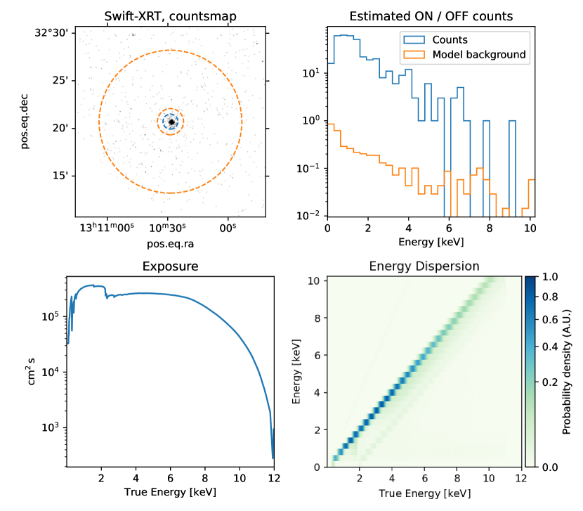
Figure 5: Swift-XRT dataset representation after energy bin grouping to avoid a background spectra dominated by zeros. (a) Swift-XRT image of OP 313. Blue circle and orange annulus show the signal and background extraction regions, respectively. (b) Distribution of events for both regions as a function of energy, corrected for the different region sizes. (c) Swift-XRT exposure (effective area $\times$ livetime) as a function of true energy. (d) Swift-XRT energy dispersion matrix (also known as redistribution matrix or migration matrix).

3.4 Swift-UVOT data reduction

The Ultraviolet/Optical Telescope (UVOT, Roming et al. 2005) onboard the Swift satellite is a diffraction-limited $30\,$cm modified Ritchey-Chrétien telescope with a limiting magnitude of $22.3$ in $1\,$ ks exposures. The CCD detector, based on XMM-Newton’s CCD (MIC) detectors, operates in photon counting mode over the range of $170$ to $650\,$ nm with 7 filters (V, B, U in the visible band; UVW1, UVM2, UVW2 in the UV band; and a white or full-passband filter).

Data reduction for Swift-UVOT is performed using heasoft v6.32.1 and the Python package photutils (Bradley et al. 2022). After downloading the target images from HEASARC’s repository, we stack images from different filters, aligning them using their world coordinate system (WCS) solutions to maximize the signal-to-noise ratio. This approach helps define the source and background regions accurately, even for dim targets, and allows to better mask potential sources in the field that might bias the background extraction. The source extraction region is defined as a circular aperture with a radius of $5\,$ arcsec, initially centered on the nominal position of OP 313 and adjusted based on centroid calculations on the stacked image. A background extraction region is then defined as an annulus with an inner radius of $12.5\,$ arcsec and an outer radius of $40\,$ arcsec, centered on the source region. Bright point-like sources in the FoV, identified by photutils, are accounted for by adding small ’masking’ circles to the background region file. An illustration of this method, including a cutout of the Swift-UVOT images for different filters, is shown in Figure 6. OP 313 is a distant, strongly Doppler-boosted source that appears point-like in most energy bands, including optical and UV. Consequently, UVOT data are analyzed using the same strategy used for XRT and NuSTAR. The result is the production of PHA source and background files (containing the integrated number of counts, single channel) for each filter. UVOT Response files (RSP) are downloaded directly from CALDB.

3.4.1 Dataset and IRFs

In imaging mode (i.e., without using the grisms) and for point-like sources, we treat UVOT as a single-channel detector with a response determined by the selected photometric filter. The RSP files provide effective area information for each filter (see Figure 6, second row). A dummy redistribution matrix is generated on the fly to match gammapy’s expected format definition. These redistribution matrices consist of a row of constant values, indicating that all photon energies contribute to the single channel of the detector.

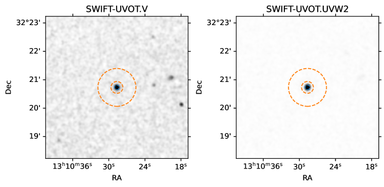
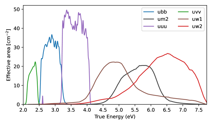
Figure 6: First row: Swift-UVOT images in two of the photometric filters available for the first selected night, with signal and background extraction regions indicated by blue and orange dashed circles and annuli, respectively. Second row: Effective collection area for each of the available Swift-UVOT filters.

3.5 Liverpool-IO:O data reduction

The Liverpool Telescope (LT, Steele et al. 2004), located on the Canary island of La Palma, is a fully robotic 2-meter telescope operated by Liverpool John Moores University. Its robotic capabilities allow for seamless transitions between different observing programs and instruments, which is crucial for time-sensitive observations of transient phenomena such as $\gamma$-ray bursts and supernovae. The IO:O (Infrared-Optical:Optical, see Barnsley et al. 2016) camera on the LT is equipped with a charge-coupled device (CCD) and a range of photometric filters. This camera includes a complete Sloan filter set: $u$, $g$, $i$, $r$, $z$, making it a valuable lower-energy complement to the Swift-UVOT.

We developed a custom data analysis pipeline using the photutils Python package to process LT IO:O calibrated images through differential aperture photometry. This pipeline reduces each image into a SpectrumDatasetOnOff compatible format in gammapy, calculating signal and background counts in ON and OFF regions, respectively. The exposure or instrument response is estimated with the same images, using a differential photometry technique consisting on measuring the flux of several calibration stars in the FoV and comparing it to their known flux densities in reference catalogs.

3.5.1 Calibration stars

For each image, the pipeline utilizes the WCS information in the FITS header to identify potential calibration stars. These stars are matched with a clean star sample from the SDSS-DR18 catalog (Almeida et al. 2023), downloaded using astroquery with a custom SQL query to select all bright stars (m${}_{u,g,r,i,z}<\,$21) in the FoV of the LT images, except: those with non-clean flags, stars close to the edges of the SDSS images, stars affected by cosmic rays, blended stars with non-robust photometry, those with large psf magnitude errors or saturated pixels. An additional query to the Pan-STARRS PS1 catalog (Chambers et al. 2016; Flewelling et al. 2020) is performed to remove variable stars, as this catalog provides a measurement of the star magnitude dispersion (in bands $g$, $r$, $i$ and $z$) for different observations of the same field. For each of the surviving stars (9 for our images), we assemble an astropy Table object containing the coordinates, magnitudes in the five selected bands and errors in the magnitudes. The magnitudes reported in the SDSS-DR18 are in the AB system, therefore conversion to flux densities is given by:

$$m_{\mathrm{AB}}=-2.5\log_{10}\left[\frac{F_{\nu}}{\mathrm{erg\,cm^{-2}\,s^{-1}\,Hz^{-1}}}\right]-48.60$$ (2)

3.5.2 Exposure estimation

The expected number of excess counts $N_{\text{src,tot}}$ for an ON/OFF dataset in a given energy window can be expressed, following Eq. 1, in terms of the exposure $\mathcal{E}(E_{\rm true})$ and the differential spectrum $\phi(E_{\rm true})$ as:

$$N_{\text{src,tot}}=\int_{E}\mathcal{R}(E,E_{\rm true})\ast\left[\mathcal{E}(E_{\rm true})\times\phi(E_{\rm true})\right]\,dE_{\rm true}.$$ (3)

For optical ground-based instruments, characterizing $\mathcal{E}(E_{\rm true})$ is complex due to the need to account for both optical elements and atmospheric effects, the latter particularly hard to assess and only accounted for as an energy-averaged scaling factor of the exposure which is derived directly from star photometry. We approximate the energy-dependence of the exposure by the detector throughput curves provided in Barnsley et al. (2016), consisting of the product of filter transmission times cryostat transmission times CCD quantum efficiency (see Figure 7). This approximation assumes that the photometric band is narrow enough for the source spectrum to be approximated by the photon density $F_{\nu}/\nu_{c}$, where $\nu_{c}$ is the effective frequency of the photometric band and $F_{\nu}$ is the flux density. Rewriting Eq. 3 in terms of wavelength, we get:

$$N_{\text{src,tot}}\simeq\frac{F_{\nu}\bar{\mathcal{E}}}{h\lambda_{c}}\int_{\lambda}T(\lambda)\,d\lambda,\quad\text{where}\ \lambda_{c}=\frac{\int_{\lambda}T(\lambda)\lambda\,d\lambda}{\int_{\lambda}T(\lambda)\,d\lambda}.$$ (4)

For each image, multiple stars are used to combine exposure estimates into a single value using a weighted average. The weights are the inverse of the estimated exposure variance. The final error on the exposure is obtained by adding the statistical uncertainty from the weighted average in quadrature to the standard deviation of all measurements:

$$\langle\bar{\mathcal{E}}\rangle=\frac{\sum_{k}\frac{\bar{\mathcal{E}}_{k}}{\sigma_{\bar{\mathcal{E}}_{k}}^{2}}}{\sum_{k}\frac{1}{\sigma_{\bar{\mathcal{E}}_{k}}^{2}}}\pm\sqrt{\frac{1}{\sum_{k}\frac{1}{\sigma_{\bar{\mathcal{E}}_{k}}^{2}}}+\sum_{k}(\bar{\mathcal{E}}_{k}-\langle\bar{\mathcal{E}}\rangle)^{2}}.$$ (5)

The exposure is then defined as $\mathcal{E}(E)=\langle\bar{\mathcal{E}}\rangle\times T(E)$, where $T(E)$ is interpolated from the known detector throughput dependency on wavelength, $T(\lambda)$.

3.5.3 Dataset and IRFs

For the LT IO:O observations of OP 313, we constructed SpectrumDatasetOnOff-style datasets, integrating photons over a region in the sky where the source is located for each filter (see Figure 7). This approach resulted in 1D datasets for each image, losing spatial information. The exposure is estimated using the method described earlier, with the RMF generated following the same process as in UVOT, consisting of a row of constant values due to the single-channel nature of each image.

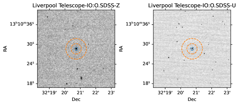
Figure 7: Top row: LT IO:O images in two of the photometric filters available for the first selected night, with the signal and background extraction regions represented by blue and orange dashed circles and annuli, respectively. Bottom row: Throughput for each of the available LT IO:O bands (transmission of the filter multiplied by the cryostat window transmission, CW, and the quantum efficiency of the CCD, QE), used to shape the energy dependence of the exposure in LT. The curves for the quantum efficiency multiplied by the cryostat, and for the cryostat alone are shown for completeness.

In contrast to space-borne photon-counting instruments, the flux calibration relies on differential photometry using calibration stars within the FoV. Variations in star spectra introduce systematic uncertainties in the effective areas. In a classical analysis method, based on flux point generation, these systematics are commonly added in quadrature to the statistical uncertainty.

In the forward-folding approach described here, an alternative method is utilized to include normalization models for each dataset or each filter (e.g., using a PiecewiseNormSpectralModel with normalization factors defined at filter-center energies). Gaussian priors are applied to account for the measured systematic uncertainties, with the widths of the Gaussian priors set to the standard deviation of the relative errors in the exposure with respect to the calculated mean. These relative errors range from less than $0.1\,$mag for the $z$- and $i$-bands to more than $0.3\,$mag for the $u$-band, where fewer reference stars are detectable. A more detailed discussion on the practical differences between the two methods and the effect of adding the systematic in quadrature to the statistical uncertainty is provided in Appendix D.

4 Results

4.1 Summary of observational data and analysis

We present the results from the broadband emission analysis of OP 313, spanning from optical to high-energy $\gamma$ rays. The instruments used, listed in decreasing order of energy coverage, are: Fermi-LAT, NuSTAR, Swift-XRT, Swift-UVOT, and the LT with the IO:O camera. Our analysis aims to interpret the data in a multi-wavelength context and evaluate the capabilities of our new multi-wavelength data management workflow. Before testing broadband modeling of the joint dataset, we carried out a technical validation of the analysis of data for each instrument separately, comparing in each case the spectral reconstruction of gammapy against that of the analysis tools native to each instrument. The details of this validation can be found in Appendix C. This section is divided into three parts:

1. Phenomenological Broadband Emission Model: We define the model for the broadband emission of OP 313, which also serves as a benchmark for the analyses.

2. Comparison of Fitting Approaches: We compare the results obtained from the canonical flux point fitting method with those from the forward-folding approach.

3. Physical Interpretation of Emission: We discuss the physical implications of the emission model and its consistency with the observed data.

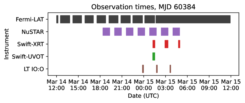
Figure 8: Temporal coverage of the first observation night with the different participating instruments.

4.2 Broadband emission modeling

4.2.1 Emission components

To model the broadband emission from OP 313, we employed a phenomenological approach using two power-laws with exponential cut-offs with index $\alpha=1$ fixed:

$$\phi_{i}(E)=\phi_{0,i}\left(\frac{E}{E_{\text{ref},i}}\right)^{-\Gamma_{1,i}}\left(-(\lambda E)^{\alpha}\right),\quad i\in\{LE,HE\}.$$ (6)

In this model, $\phi_{LE}(E)$ represents the synchrotron emission (low energy component), and $\phi_{HE}(E)$ represents the inverse Compton emission (high energy component) in a simplified leptonic scenario. The $\lambda$ parameter refers to the inverse cut-off energy.

4.2.2 Absorption components

Absorption models were applied as follows:

• ISM Extinction: Relevant for optical and especially UV energies. Given OP 313’s Galactic latitude of $+83.34^{\circ}$ and a color excess of $E_{B-V}\approx 0.0125$ (Schlegel et al. 1998), interstellar medium (ISM) extinction is minimal until about $\leavevmode\nobreak\ 10$ eV, where the medium quickly becomes optically thick. At $\sim 5\,\text{eV}$ (UVOT’s UVM2 filter), the transparency is still about 90% according to the ISM absorption model by Cardelli et al. (1989).

• Hydrogen I Absorption: Relevant for X-ray energies below $\sim 1\,\text{keV}$. Parameterized using the HI column density, following Wilms et al. (2000). For OP 313, the HI column density is approximately $1.25\times 10^{20}\,\text{cm}^{-2}$ (HI4PI Collaboration et al. 2016).

• EBL Absorption: Significant at energies above $\sim 10\,\text{GeV}$. We use the model from Saldana-Lopez et al. (2021), which can be regarded as an update over Domínguez et al. (2011).

4.3 Forward folding fitting method

We employed two distinct fitting methodologies to analyze the data from the participating instruments:

1. Flux Point Fitting: This traditional method fits the model to observed flux points derived from analyzing each instrument’s data separately. Although it simplifies the fitting and can be computationally faster, it is observed to be more sensitive to the choice of initial parameters. Additionally, this approach may introduce errors due to differences in flux estimation and instrument calibration methodologies. It also overlooks upper limits and correlations between flux points, potentially affecting the accuracy of the fit.

2. Forward Folding Technique: This method fits the model directly to the counts or event data from the instruments, incorporating the IRFs in each iteration. It accounts for background components and full instrumental effects, leading to improved accuracy and, as observed, better convergence compared to the flux point fitting method.

Figure 9 illustrates the best-fit models and their confidence bands for both fitting methods, while Figure 10 shows the correlations between the model parameters estimated from the covariance matrix for each fit. Both methods yield consistent results with well behaved residuals across the electromagnetic spectrum, confirming that the phenomenological model effectively captures the emission from OP 313 from optical to the $\gamma$-ray band. However, the forward folding technique shows better exploitation of the data, as it is able to use data beyond the last significant bins in both NuSTAR and Fermi-LAT.

Other notable differences between the two methods include the treatment of instrumental effects and background components, more accurate in the forward folding case as the method directly incorporates energy redistribution and provides a more uniform representation of the emission in the observed counts space. In the NuSTAR case, bins for which the effective area of the instrument is approximately zero can still be of use as they can effectively constrain the instrumental background model. As opposed to directly fitting instrumental background components during the forward folding, the classical method inadequately performs a fit to ‘flux points’ implying that the background is either fixed or subtracted. A similar problem occurs with Fermi-LAT skymodel, consisting on the sum of diffuse components (isotropic component, galactic diffuse emission) and a number of point-like source lying close to OP 313. In the classical method, the contributions of such components are ‘frozen’, as opposed to fitted in the forward folding. Finally, the proposed workflow reduces systematic uncertainties associated with the conversion of counts to fluxes in the optical band as information coming from different filters are indirectly accounted for in the counts-flux conversion, likely improving the accuracy of the fit.

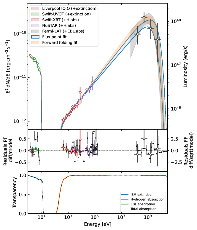
Figure 9: Joint multi-instrument forward-folding fit and joint fit using flux-points employing a phenomenological model with two distinct emission components and three absorption components. Top panel: individual datasets fitted with simple models (power-laws, log-parabolas, power-laws with exponential cutoffs) and corresponding reconstructed flux points, and joint fits (flux points, forward folding). Middle panel: Residuals, calculated as the ratio of reconstructed differential spectrum to model prediction for the flux points fit (Residuals PF, open circles), and as the significance or ratio of the difference between the excess counts and model predicted counts to the square root of the model predictions for each bin in the forward folding case (Residuals FF, small filled circles). For clarity, and due to the large amount of energy bins in the X-ray datasets, only one every 5 bins is shown for NuSTAR, and one every 3 bins is shown for XRT. Bottom panel: Multiplicative absorption components.

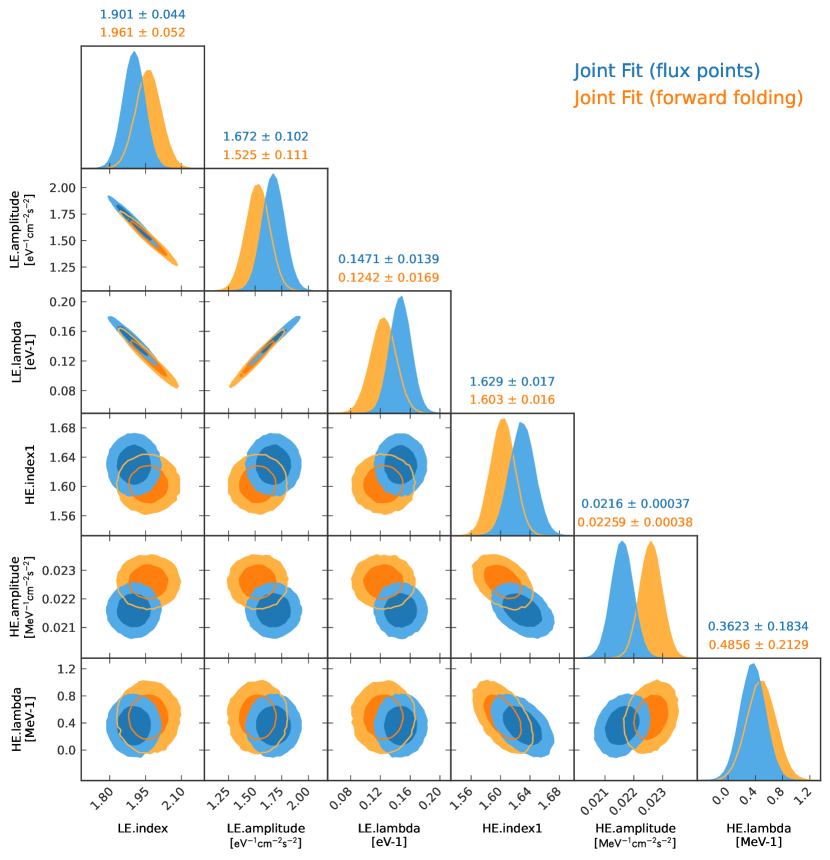
Figure 10: Corner plot showing the error ellipses calculated with a bootstrap method for the best-fit (free) parameters of the flux-point based fit and the full forward-folding joint fit. The model used for the LE is strongly degenerated because of the limited amount of available data to constrain that component.

4.4 Physical interpretation of the broadband emission

The continuous spectral connection from X-rays to $\gamma$-rays observed in Figure 9 suggests a coherent emission scenario likely originating from a single emission zone, and points to a single inverse Compton process to explain both the X-ray and $\gamma$-ray emissions.

The data also favors an external inverse Compton model for OP 313 due to the large ratio of peak energy fluxes in the high energy component of the SED to that of the low energy component (Compton Dominance). In a synchrotron-self-Compton scenario, achieving such high Compton Dominance would require too low magnetic fields and unrealistically high Doppler factors and/or electron densities. In contrast, the external Compton scenario can naturally result in large values for that ratio as electrons scatter the highly dense photon field from external components such as the accretion disk, the dusty torus or the broad line region of the AGN.

To further identify the specific external radiation field responsible for the Compton up-scattering, additional data in the VHE regime would be necessary. Observations with instruments such as LST-1 or MAGIC could provide this information. This aspect is beyond the scope of this work, and will be explored in a forthcoming publication including VHE observations from these two instruments.

5 Discussion

In the preceding sections, we evaluated a flexible data format designed to streamline both archival and analysis processes. This format, based on OGIP and the GADF initiative, integrates direct observations — such as event counts, spectra (energy distributions of counts), or spatially-resolved data cubes — with IRFs from a diverse range of instruments, from space-borne $\gamma$-ray observatories like Fermi-LAT to ground-based optical telescopes like the LT.

5.1 Flexibility and modeling capabilities

The method excels at providing flexibility for data modeling. We tested a phenomenological model with two simple power-laws with exponential cut-offs as emission components, aimed at representing synchrotron and inverse Compton emissions from a relativistic particle population in a jet. This model was complemented with fixed absorption components (extinction, neutral hydrogen, and EBL) and various background sources (diffuse radiation fields, additional sources in Fermi-LAT, and instrumental backgrounds in NuSTAR). Despite leaving free many of these additional components (normalizations of the spectral components of bright Fermi-LAT sources, Fermi-LAT isotropic and galactic diffuse components, and instrumental backgrounds in NuSTAR-A and NuSTAR-B), the minimization converged within a reasonable computing time using the proposed Forward Folding technique, offering advantages over traditional methods that rely on reconstructed flux points.

This approach is particularly beneficial for X-ray data analysis, providing a modern and flexible framework compared to older tools like xspec, whose first release dates from 1983 and is often misused to produce flux points despite not being technically designed for that purpose. In the case of NuSTAR, this is especially relevant since instrumental background models quickly develop to a very complex sum of models components, making it almost impossible to extract flux points using xspec, as it would require to remove the contribution to the total flux from each of the components. The proposed flexible format, combined with tools such as gammapy, potentially enables a 3D analysis of XRT and NuSTAR data. This could be particularly advantageous for extended sources, or for a point source on top of an extended source (e.g. a halo), especially for instruments with limited angular resolution like NuSTAR. Therefore, the method tested in this work presents natural extensions and improvements.

5.2 Main challenges and practical limits

The increased flexibility and accuracy naturally comes with trade-offs. The method involves a more complex workflow and a larger parameter space. It also requires a more detailed modeling of observational data to incorporate all effects (astrophysical and instrumental backgrounds) and has to fold spectral models with various IRFs in each iteration to predict ‘observables’ (counts, spectra, or data cubes) that are fit to the data. This complexity results in a higher computation time, and practical limits for the method’s application are yet to be fully assessed.

For Fermi-LAT, the current implementation assumes that the PSF depends only on energy, and is constant within the FoV. This is a potential limitation with respect to its native analysis pipeline, Fermitools. Fortunately, for bright point-like sources like OP 313, where the contribution of other sources in the FoV is almost negligible, this effect should be small. Being gammapy an active developed tool, this drawback may be addressed in the future.

5.3 Considerations for optical instruments

In the optical band, we tested a simplified IRF implementation tailored for relatively broad ‘filter’ photometry. This approach represents a significant improvement over classical methods, which often just multiply the measured flux densities obtained through differential photometry techniques by an effective frequency of the band calculated under some assumption (typically flat photon spectrum or flat energy spectrum), ignoring the actual spectrum of the source. For steep spectra like that of OP 313 in the UV band, the real photon distribution is typically skewed, shifting the effective frequency of the band.

The approximate IRFs we introduced in this work still built and used in this study omit critical factors such as how atmospheric extinction, mirror reflectivity, aging of mirror coatings, and CCD defects modify the effective band profile. Including these elements in the IRFs — though technically challenging — would improve the accuracy of the spectral reconstruction. We did not explore spectral data analysis in the optical band due to the additional complexities involved, such as calibrating both wavelengths and fluxes, which could compromise the Poisson statistics of the observed data.

6 Conclusions

The results presented in Section 4 demonstrate the effectiveness of the forward-folding technique for astrophysical data analysis in the context of complex multi-wavelength studies involving several instruments. This method not only shows that it is possible to organize, store, and analyze data from different instruments together in a consistent manner, but offers practical advantages over the classical flux-point fitting technique in terms of robustness. Furthermore, it allows for a more accurate statistical comparison of different modeling hypotheses, thereby simplifying the interpretation of the physical processes at play for a source like the FSRQ OP 313.

The resulting multi-instrument datasets and analysis code are stored in a format that is convenient for distribution and archiving. This format not only facilitates the reproduction of the results obtained in this specific study, but also supports further research on OP 313 with public datasets, as well as serve to make future validation tests for gammapy. Future work could involve detailed modeling of the spectral energy distribution using physical models through codes such as jetset (Tramacere et al. 2009, 2011), agnpy (Nigro et al. 2022), Bjet_MCMC (Hervet et al. 2024), or SOPRANO (Gasparyan et al. 2022, 2023).

This study provides a largely static view of OP 313 for two specific nights. Including variability studies and time-evolving models that account for particle injection and cooling will enhance our understanding of the emission of the source in particular and blazars in general. In this regard, the proposed simplified handling of instrument datasets will ensure greater consistency and reduce errors compared to classical methods that use data in disparate formats, as well as hopefully providing one of the first comprehensive multi-wavelength blazar datasets built over standarized data formats and open-source analysis tools.

Appendix A Software description and data repository

This work is based on the open-source analysis tool gammapy and open data formats initiatives (GADF, OGIP). Only two new code implementations were required to conduct the analysis as presented in this manuscript. The first is a reader for standard OGIP files generated by HEASARC’s native tools like uvot2pha, xrtproducts, and nuproducts. Originally developed by Giunti & Terrier (2022) for XMM, it was extended to also support NuSTAR, Swift-XRT, and Swift-UVOT. The second implementation is a set of Python classes that perform an optical point-like reduction photometry of Liverpool Telescope IO:O data, producing OGIP files from optical images using a set of reference stars with known photometry from Sloan’s SDSS DR18 and PanSTARR’s PS1 catalogs.

Additionally, we provide Jupyter notebooks (Perez & Granger 2007; Ragan-Kelley et al. 2014) to illustrate the details of the construction of the gammapy-compliant datasets, as well as the analysis of each individual dataset and the joint analysis of the broadband datasets. These codes, along with the resulting gammapy-compliant data files, are available in a GitHub repository (Nievas 2024) for easy access and reproducible results. The structure of this repository is as follows:

• Notebooks/DatasetGenerator

• Notebooks/DatasetAnalysis

• Helpers

• Models

• Figures

Within the Notebooks/DatasetGenerator/ directory (with one subdirectory for each night of observations), we stored notebooks (one per instrument) that compile all the steps to generate the gammapy-compliant 1D and 3D binned datasets, as described in Section 3. Similarly, Notebooks/DatasetAnalysis/ contains notebooks with the analysis of the datasets from individual instruments and the joint analysis of the multi-wavelength (MWL) datasets. The Helpers/ directory contains functions for generating gammapy native multiplicative models for dust extinction, neutral hydrogen, and EBL absorption. It also includes classes for fetching photometry data from the PS1 and SDSS DR18 catalogs, as well as various file handling and plotting functions used across the analysis notebooks. The Models/ directory contains the tabular absorption models for EBL (Domínguez et al. 2011; Saldana-Lopez et al. 2021), the neutral hydrogen absorption exported from xspec’s TBabs model (NASA 2024a), and the dust extinction extracted from xspec’s redden (NASA 2024b). Finally, the Figures/ directory (one subdirectory per observing night) contains plots and figures presented in this work.

Appendix B Background estimation methods for NuSTAR

Two different methods for estimating the background in 1D datasets were explored for NuSTAR observations. The first method is the general Poisson or OFF background estimate. This method makes minimal assumptions about the structure of the background spectra, primarily that the background spectrum is identical in the OFF region as in the ON region. While this approach offers significant flexibility, it has the downside that Poisson fluctuations can dominate the often weak emission from the source, particularly at higher energies. Moreover, the assumption of Poisson statistics requires all background spectral bins to have non-zero counts to ensure a correctly defined likelihood function. This can pose a problem for photon-counting instruments like NuSTAR, especially when integrating over short exposure times. To mitigate issues arising from zero-count bins, it often becomes necessary to group the data into coarser energy bins, which can compromise spectral resolution.

The second method involves modeling the background, a technique extensively used in the analysis of data from instruments like Fermi-LAT, where detailed background models such as diffuse galactic emission maps and isotropic emission spectra have been developed. In this work, we employ a similar approach for NuSTAR by using instrumental background spectral models generated by the nuskybgd tool. This method provides an alternative to the Poisson background estimate by incorporating a more structured model of the instrumental background into the analysis.

A direct comparison between the reconstructed spectra of the FSRQ OP 313 obtained using the two methods is shown in Figure 11(b), with the OFF background estimation results depicted in blue and the model background prediction results in black. Additionally, Figure 12(b) presents the best-fit parameter error ellipses for both methods. The comparison reveals that at lower energies, where photon statistics are robust, the results from both methods are fully compatible. However, discrepancies begin to emerge at energies above 30 keV. Notably, in the 60–70 keV range, the OFF background estimate only provides an upper limit (with less than a 2$\,\sigma$ excess), while the model background based analysis continues to reconstruct a flux point with a significance exceeding 2$\,\sigma$.

These findings suggest that while both methods are viable, the choice of background estimation method can significantly impact the results at higher energies, particularly when the source signal is weak compared to the background. The model background method, with its more sophisticated modeling of the instrumental and astrophysical background, may offer advantages in these regimes, potentially yielding more accurate spectral reconstructions where the OFF background method falls short.

Appendix C Dataset analysis validation

This appendix shows the comparison between the analyses conducted using native tools specific to each instrument (i.e. xspec for NuSTAR and XRT, Fermitools/enrico for Fermi-LAT) and those performed on the OGIP- and GADF-compliant datasets using gammapy. This comparison is needed for validating the consistency and reliability of the gammapy-based analysis, and will turn crucial to later extend the full statistical forward folding technique across different wavelength regimes.

For high-energy instruments like Fermi-LAT, NuSTAR, and Swift-XRT, we directly compared in Figure 11 the best-fit spectral energy distribution confidence bands and corresponding flux points. To keep the comparison straightforward and the parameter space limited to just two variables, we used a simple power-law in each band, with either EBL absorption in $\gamma$ rays or neutral hydrogen absorption in X-rays. Even though Fermi-LAT $\gamma$-ray data hints significant curvature in that band, using a simple model is enough to test the validity of the method, and only a power-law with exponential cut-off was used in Figure 9 for the broadband analysis.

The results shown in Figures 11(a), 11(b) and 11(c) indicate that the best-fit model and contours obtained with gammapy are indistinguishable from those obtained with the native tools, demonstrating the potential of gammapy as a multi-wavelength data analysis framework.

In addition, we show in Figure 11(b) the spectral reconstruction with both the instrumental background and the Poisson background estimate, well matching below $\sim 30$  keV. We note however that xspec has two severe limitations. The first is linked to the definition of a the power-law, whose pivot energy in xspec is fixed to $1\,$keV and cannot be changed. To avoid impacting the results with a reference energy that is outside the energy range of NuSTAR, we redefined the power-law so that the normalization is done with respect to the the integral flux in the $3-70\,$keV band, instead of at a specific energy. The second limitation is that xspec is not designed to produce flux points as we noted in Section 5.1, and only in simple cases with few spectral components (NuSTAR and Swift-XRT when doing an OFF background analysis with Poisson background statistics) it was feasible to estimate some sort of flux points for different energy bins. For more sophisticated cases, such as NuSTAR with the complex instrumental background model produced by nuskybgd, the flux points estimated with xspec do not correspond to the source component but to the total sky model, including the systematic background. Removing the additional background components (which are not fixed) is not trivial, therefore we only report in Figure 11(b) the SED confidence band from xspec, without the flux points. We also checked the parameter error contours in the amplitude vs spectral index parameter space in Figure 12, noting a very good agreement for the three instruments.

Table 1: Comparison of parameter values for the best-fits of the native tools (fermitools+minuit/migrad for Fermi-LAT data, xspec’s Levenberg-Marquardt algorithm for NuSTAR and Swift-XRT) with the same results obtained with gammapy with the default minuit/migrad as minimizer and algorithm. For simplicity, a classical power-law with absorption with amplitude defined as the photon density at a reference energy was used for Fermi-LAT and Swift-XRT (including also EBL absorption for Fermi-LAT following in this case Domínguez et al. (2011) as it is included in the Fermitools, and neutral hydrogen for Swift-XRT as implemented in xspec’s TBabs code). For NuSTAR, a power-law with integral as amplitude parameter was utilised as xspec does not allow to change the default reference energy, which is fixed at $1\,$keV and therefore out of the energy range of the instrument. Switching to migrad in xspec showed a completely negligible impact on the estimated minima.

	Fermi-LAT		NuSTAR A+B		Swift-XRT
	@$1\,$GeV		$3-70\,$ keV		@$1\,$keV
	amplitude	index	integral flux	index	amplitude	index
native	$1.00\pm 0.23$	$2.01\pm 0.16$	$6.30\pm 0.12$	$1.633\pm 0.030$	$9.28\pm 0.53$	$1.671\pm 0.075$
gammapy	$0.98\pm 0.23$	$2.05\pm 0.19$	$6.33\pm 0.12$	$1.630\pm 0.030$	$9.09\pm 0.53$	$1.667\pm 0.077$
scale	$\times 10^{-11}$		$\times 10^{-4}$		$\times 10^{-4}$
units	$\mathrm{MeV^{-1}s^{-1}cm^{-2}}$		$\mathrm{s^{-1}cm^{-2}}$		$\mathrm{keV^{-1}s^{-1}cm^{-2}}$

(a) Fermi-LAT.

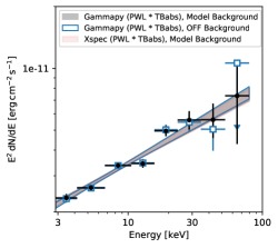
(b) NuSTAR

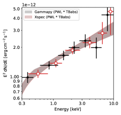
(c) Swift-XRT

Figure 11: Best-fit power-law models (with EBL absorption in Fermi-LAT and neutral hydrogen absorption for NuSTAR and Swift-XRT) fitted to each dataset with native tools (xspec or Fermitools depending on the case) and gammapy. For reference, the spectral reconstruction with the OFF Background estimate in NuSTAR (second panel) is shown in blue for reference. Upper limits are calculated at a 95% confidence level from the cstat/wstat likelihood profiles.

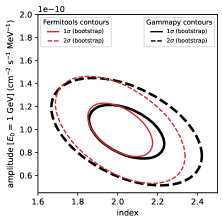
(a) Fermi-LAT.

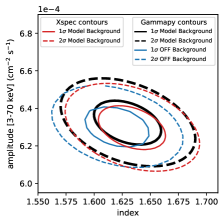
(b) NuSTAR

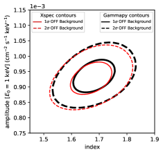
(c) Swift-XRT

Figure 12: Parameter error ellipses on the amplitude (integral flux for NuSTAR) and spectral index for the power-law fit to the Fermi-LAT, NuSTAR A+B and Swift-XRT datasets. Contours in black correspond to gammapy, while the native tool contours are shown in red. For NuSTAR, the contours obtained with the Poisson or OFF background estimate are shown in blue for reference.

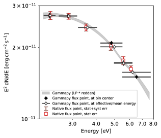
(a) Swift-UVOT

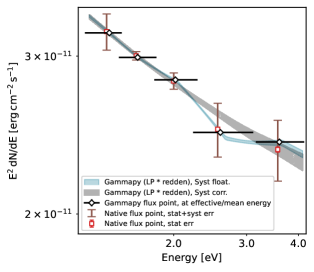
(b) Liverpool Telescope IO:O

Figure 13: Best-fit spectra and SED points reconstructed using gammapy using counts and IRFs and with native tools using magnitudes or flux densities and multiplying by the effective filter frequency center. The emission in gammapy is modelled with a log-parabola with dust extinction. Flux points in gammapy are evaluated over the geometrical center of the bin (black filled circles) and at the effective mean energy of the band with open diamond symbols (under the assumption of a flat source photon spectrum, to be roughly comparable to the classical method). LT datasets from the same filter were stacked together using gammapy’s stack_reduce method, that co-adds the counts, background and exposures for datasets with compatible energy axes. For reference, weighted average fluxes for the native flux points are shown in colored red boxes, while brown error bars depict the total error once incorporating systematic uncertainties.

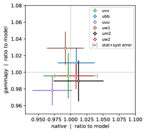
(a) Swift-UVOT

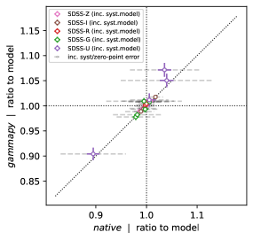
(b) Liverpool Telescope IO:O

Figure 14: Comparison of reconstructed ‘relative’ flux values using native photometry tools (which calculate source magnitudes or flux densities and multiply by the filter’s effective frequency) and those obtained with gammapy (using counts and instrument response functions). All ‘relative’ fluxes are shown as a ratio to the best-fit gammapy model of the joint datasets, evaluated at the corresponding point energy.

Appendix D Systematic Uncertainties in Liverpool Telescope Data

In classical analysis, systematic uncertainties related to errors in the zero-point estimation (star-to-star variations) are typically propagated in quadrature to the final error estimate of the source flux. While this method is model-independent, it does not take full advantage of the detailed broadband spectrum of the source, which becomes more apparent as additional data across different energy bands are incorporated.

In this work, we explore an alternative approach using the PiecewiseNormSpectralModel in gammapy. This model adds an energy-dependent multiplicative component to our source’s spectral model, allowing the normalization parameters at each fixed energy node to be free. To avoid creating a highly degenerate model by leaving these parameters completely unconstrained, we impose Gaussian priors on each normalization factor. These priors are centered at 1, with widths corresponding to the systematic uncertainties arising from star-to-star variations in the calculated exposure.

When this component together with the source spectrum is fitted to the data, it causes a deformation of the assumed spectrum (e.g., a log-parabola), enabling the model to better align with the actual measurements (excess counts) by subtly adjusting the shape of the spectrum (see 13(b), light gray curve and black diamond markers). By removing this component, we can recover the underlying estimate of the true spectrum (dark gray) ,free from the influence of systematic errors. For clarity, in this figure we stacked together observations using the same filter, which in gammapy it is technically implemented in the stack_reduce method by co-adding the counts, background and exposures for datasets with compatible axes. The equivalent stacking is achieved for the native (classical) analysis by performing a weighted average of the flux point values, where the weights are set to the inverse of the square of the statistical errors of the points.

This correction effect is also illustrated in Figure 14(b), where arrows illustrate how the flux points would shift if the systematic components were excluded from the spectral model. The comparison between the two sets of spectra and flux points, one including the systematic component and one corrected for it, is shown in Figure 13(b).

Appendix E Second night analysis (MJD60384)

The body of this manuscript primarily discusses the methodology used to create gammapy-compatible datasets, with data from the first night of NuSTAR observations (March 4th, 2024, MJD 60373) presented as an example of the reconstruction achievable using our analysis framework. In this appendix, we briefly report the results of applying the same analysis to the second night of NuSTAR observations (March 15th, 2024, MJD 60384) for which the temporal coverage of the instruments is shown in Figure 15.

Figure 15: Temporal coverage of the first observation night with the different participating instruments.

To keep this section short and focused on the final results, we focus on the two main figures from Section 4.4. The first figure is the best-fit models, shown in Figure 17, using the same sum of two power-laws with exponential cut-offs as in Figure 9. The corresponding corner plot, representing the error ellipses for each pair of free model parameters for the source emission component, is displayed in Figure 18. Compared to Figure 10, we observe a similar degree of degeneracy between the parameters for the low-energy (LE) component, and overall, there is a good agreement between the two fitting techniques for all parameters. However, in this case, the forward folding fit appears to better constrain the inverse of the cutoff energy $\lambda$ of the high-energy (HE) component, which is reflected in the figure as a more oblate ellipse. Regarding the parameters, the HE component seems to exhibit a slightly harder spectrum than on the first night.

We note however that there is some tension between Swift-UVOT and Liverpool IO:O, and between Swift-XRT and NuSTAR. We considered two possible causes of this. The first one is related to the observing times themselves in combination with intra-night source variability, as XRT observations are concentrated around the second half of NuSTAR only. This however is not supported by the relatively stable spectra in the Fermi-LAT, NuSTAR and Liverpool bands between the two nights. A more likely cause seem to be a degraded pointing of Swift satellite after one IRO (gyroscope) became noisy in Summer 2023 and then again in Spring 2024, leading to an increase chance of star tracker “loss of lock” after long slews. This is in fact hinted in our data from the Swift-XRT, whose integrated PC-mode image show a larger PSF and slightly larger field noise than that of the first night. And it is even more evident from the single UVOT exposure in filter UM2, where OP 313 image is far from round, and even not fully contained in the predefined source region size, as seen in Figure 16. While the effect should be less severe in XRT than in UVOT due to the larger intrinsic PSF, we believe this possible loss of lock in the star tracker during our observations may have led to a significant underestimation of the source flux in both instruments.

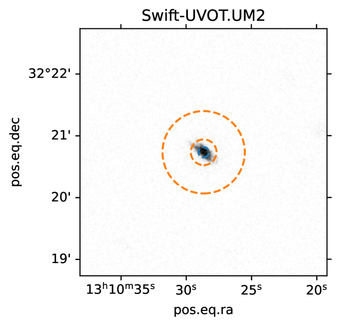
Figure 16: Swift-UVOT image with filter UM2 on the night of MJD60384. Blue circle indicate the standard ON integrated region, while the orange circles indicate the annulus for the background extraction.

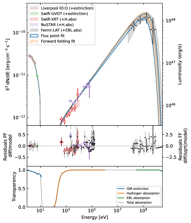
Figure 17: Joint multi-instrument forward-folding fit and joint fit using flux-points from the night of March 15, 2024 (MJD60384) with the similar structure as in Figure 9. Note that Swift data were affected by a severe “loss of lock” problem that night.

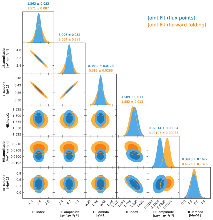
Figure 18: Corner plot showing the error ellipses calculated with a bootstrap method for the best-fit (free) parameters of the flux-point based fit and the full forward-folding joint fit. The model used for the LE is strongly degenerated because of the limited amount of available data to constrain that component.