Alternative representation of the large deviation rate function and hyperparameter tuning schemes for Metropolis-Hastings Markov Chains

Abstract.

Markov chain Monte Carlo (MCMC) methods are one of the most common classes of algorithms to sample from a target probability distribution $\pi$. A rising trend in recent years consists in analyzing the convergence of MCMC algorithms using tools from the theory of large deviations. One such result is a large deviation principle for algorithms of Metropolis-Hastings (MH) type (Milinanni & Nyquist, 2024), which are a broad and popular sub-class of MCMC methods.

A central object in large deviation theory is the rate function, through which we can characterize the speed of convergence of MCMC algorithms. In this paper we consider the large deviation rate function from (Milinanni & Nyquist, 2024), of which we prove an alternative representation. We also determine upper and lower bounds for the rate function, based on which we design schemes to tune algorithms of MH type.

1. Introduction

Sampling from a target distribution $\pi$ is a fundamental task in many applied fields, spanning from computational biology and statistical mechanics, to epidemiology and ecology [And+03, AG07, RC04]. A setting where sampling is predominant is that of Bayesian statistics. In fact, a direct computation of the Bayesian posterior distributions in practical applications is typically computationally prohibitive, and a valid alternative to the direct computation consists in sampling from the posterior distribution.

Markov chain Monte Carlo (MCMC) methods are a wide and popular class of sampling algorithms. These methods generate a Markov chain that has $\pi$ as invariant distribution [RC04]. One of the most common algorithms in this class is the Metropolis-Hastings (MH) algorithm, which is based on a mechanism of proposing a state for the next element of the chain, and then accepting or rejecting the proposal. Different choices of proposal mechanism lead to different algorithms of MH type [Met+53, Has70]. Examples of algorithms that fall in the MH category are the Independent Metropolis-Hastings (IMH) algorithm, the Random Walk Metropolis (RWM) algorithm, the Metropolis-adjusted Langevin algorithm (MALA) and Hamiltonian Monte Carlo (HMC) [Tie94, RC04, MT96, SFR10, Bes94, RR98, RT96, Dua+87].

In order to design efficient sampling algorithms, it is of crucial importance to perform a theoretical analysis of the underlying Markov processes. In fact, in applied problems a blind use of off-the-shelf sampling algorithms can require excessively large computation times. A theoretical understanding of the convergence properties of MCMC methods helps us in designing algorithms that successfully perform the sampling task with a reasonable computational effort. The Monte Carlo literature already provides a variety of tools to perform convergence analysis of MCMC algorithms. Some of the more classical tools for convergence analysis include: spectral gap, asymptotic variance, mixing times, functional inequalities [BR08, Ros03, DHN00, Fra+10, Fri+93, HHS05, And+22, And+23, Pow+24].

In recent years, we have witnessed a growing trend of using the theory of large deviations to analyze the speed of convergence of sampling algorithms. This approach is based on the seminal work by Donsker and Varadhan [DV75, DV75a, DV76], and consists in deriving a so-called large deviation principle (LDP) for the empirical measures associated with the algorithms’ underlying Markov processes. More in detail, if an algorithm generates discrete time Markov chains $\{X_{i}\}_{i\in\mathbb{N}}$, as the algorithms of MH type, the corresponding empirical measure is the random probability measure defined as

$$L^{n}(dx)=\frac{1}{n}\sum_{i=0}^{n-1}\delta_{X_{i}}(dx).$$

If the algorithm is well-designed, the sequence of empirical measure $\{L^{n}\}$ converges almost surely to the target $\pi$, in the weak topology. By saying that the sequence of empirical measures $\{L^{n}\}$ satisfies a large deviation principle with speed $n$ and some rate function $I$, we mean, roughly speaking (see Section 1.3 for a formal definition), that the convergence $\lim_{n\to\infty}L^{n}=\pi$ is exponentially fast. In addition, the rate function $I$ provides important information on the corresponding speed of convergence. The fundamental concept is: larger rate function implies faster convergence of the sampling algorithm.

Whereas more classical convergence tools mainly describe the distribution of the $i$-th iterate of the Markov chain, $X_{i}$, this large deviations approach accounts for the information on the time averaging effect of the empirical measure. We have to keep in mind that the empirical measure is what we use in practice when we compute Monte Carlo estimates. For example, we typically approximate the integral $\int f(x)\pi(dx)$ with the empirical average $\frac{1}{n}\sum_{i=0}^{n-1}f(X_{i})$. Note that such empirical average corresponds to integrating the function $f$ in the empirical measure, i.e., we are letting $\int f(x)\pi(dx)\approx\int f(x)L^{n}(dx)$.

The first works on large deviations for sampling algorithms appeared in the early 2010s [Pla+11, Dup+12]. In these papers the authors study the parallel tempering sampling algorithm, and notably, the use of the large deviations approach led to the design of a new sampling scheme, the infinite swapping. Later works in this line of research include [RS15, RS15a, RS16, Bie16], where the empirical measure large deviation principle is used to show that algorithms based on non-reversible Markov processes exhibit faster convergence. Further studies of the parallel tempering algorithm, and the related infinite swapping algorithm, are carried out in [DDN18] and [DW22]. In the former, the large deviation rate function is used to derive convergence properties of the two methods, while in the latter, the temperatures (hyperparameters) of these algorithms are tuned via the empirical measure LDP. In [BNS21] the empirical measures large deviation is used to study and optimize the zig-zag sampler.

The first study of algorithms of MH type in continuous state space based on the theory of large deviations is presented in [MN24]. Therein, it is studied a large deviation principle for general discrete-time stochastic processes, of which the MH algorithms are a special case. In a later work [MN24a], the LDP from [MN24] is applied to analyze specific algorithms from the MH class: the IMH, MALA and the RWM algorithms.

The large deviation rate function in [MN24] is characterized as the minimum of a relative entropy functional (also referred to as Kullback-Leibler divergence), where the minimum is taken among probability measures of a specific type. As minimizing over probability measures can be demanding, we seek for an alternative representation of the rate function. In Section 2 we provide such an alternative representation, which is dual to that in [MN24]. This new representation characterizes the LDP rate function as a maximization problem over continuous functions satisfying certain properties. Optimization problems over continuous functions can be more tractable compared to optimizing over probability measures. However, both optimizations may be challenging to compute.

To simplify the problem of computing the rate function, in Section 3 we derive corresponding explicit upper and lower bounds that are easy to compute numerically. Thanks to these bounds, we can avoid the exact computation of the rate function, and provide closed intervals to easily quantify the rate of convergence of MH algorithms.

These bounds allow us to design three tuning schemes to identify “optimal” (in the sense of leading to fastest convergence) hyperparameters for sampling algorithms of MH type. These schemes are described in Section 4, and in Section 5, in an illustrative example, we show how to use one of these schemes to tune the IMH algorithm. These are the first results on tuning algorithms of Metropolis-Hastings type based on the theory of large deviations. In future work, we will consider more complex algorithms of MH type, such as MALA and HMC. The ultimate goal is to design schemes to precalibrate algorithms of MH type in applications, where limited information on the target $\pi$ is typically available.

The remainder of the paper is organized as follows. In Section 1.1 we describe the notation used throughout the paper. In Sections 1.2 and 1.3 we describe the algorithms of MH type and the large deviations result from [MN24], respectively. In Section 2 we prove an alternative representation of the LDP rate function. In Section 3 we derive upper and lower bounds for the rate function. We then use these results to design three tuning schemes, described in Section 4. The paper ends with Section 5, where we show, with an illustrative example on the IMH algorithm, how we can use these tuning schemes to optimize the hyperparameters in MH algorithm.

1.1. Notation

Throughout this paper we will work on some probability space $(\Omega,\mathcal{F},\mathbb{P})$.

Given a Polish space $S$, $\mathcal{C}(S)$ denotes the space of continuous functions, and $\mathcal{C}_{c}(S)$ the space of continuous functions with compact support on $S$. As Polish space $S$ we will consider continuous subsets of $\mathbb{R}^{d}$, $d\geq 1$.

The space of probability measures on a Polish space $S$ will be indicated as $\mathcal{P}(S)$, and it will be metrized through the Lévy-Prohorov distance $\text{dist}_{LP}$. For any $\varepsilon>0$, $\mu\in\mathcal{P}(S)$,

$$B_{\varepsilon}(\mu)=\{\nu\in\mathcal{P}(S)\text{ s.t. }\text{dist}_{LP}(\mu,\nu)<\varepsilon\}$$

denotes the ball of radius $\varepsilon$ centered at $\mu$ in the Lévy-Prohorov metric.

With a slight abuse of notation, given a measure $\mu(dx)\in\mathcal{P}(S)$, we will denote by $\mu(x)$ its density with respect to the Lebesgue measure (if it exists).

Given $\theta,\varphi\in\mathcal{P}(S)$, we denote the relative entropy between $\theta$ and $\varphi$ as

$$R(\theta\parallel\varphi)=\begin{cases}\int_{S}\log\frac{d\theta}{d\varphi}d\theta,\quad\text{ if }\theta\ll\varphi,\\ +\infty,\;\quad\qquad\qquad\text{otherwise}.\end{cases}$$

For $\gamma\in\mathcal{P}(S\times S)$, let $[\gamma]_{1}(dx)$ and $[\gamma]_{1}(du)$ denote the first and second marginals of $\gamma(dx,dy)$, respectively. Define

(1) $$A(\mu)=\left\{\gamma\in\mathcal{P}(S\times S)\,\text{ s.t. }[\gamma]_{1}=[\gamma]_{2}=\mu\right\},$$

and let $\mathcal{Q}(\mu)$ be the set of all the stochastic kernels $q(x,dy)$ on $S$ such that $\mu$ is an invariant distribution for $q$.

Given any stochastic kernel $q(x,dy)$ and a function $u:S\to\mathbb{R}$, we define

$$(qu)(x)=\int_{S}u(y)q(x,dy).$$

1.2. The Metropolis-Hastings algorithm

Given a target distribution $\pi\in\mathcal{P}(S)$, the Metropolis-Hastings (MH) algorithm produces a Markov chain $\{X_{i}\}$ that has $\pi$ as invariant distribution. An essential element of the MH algorithm is the proposal distribution $J(\cdot|x)\in\mathcal{P}(S)$, defined for all $x\in S$. Different proposals lead to different MH algorithms.

If at the $i$-th iteration, the state of the chain is in $X_{i}=x_{i}\in S$, the algorithm generates a proposal $Y_{i+1}$ for the next state of the chain, $X_{i+1}$, by sampling from $J(\cdot|x_{i})\in\mathcal{P}(S)$. The proposal $Y_{i+1}$ is then accepted or rejected based on the Hastings ratio

$$\varpi(x,y)=\min\left\{1,\frac{\pi(y)J(x|y)}{\pi(x)J(y|x)}\right\}.$$

With probability $\varpi(x_{i},Y_{i+1})$ we accept the proposal and set $X_{i+1}=Y_{i+1}$. Under rejection, with probability $1-\varpi(x_{i},Y_{i+1})$, we set $X_{i+1}=x_{i}$.

The MH algorithm is illustrated in Algorithm 1.

Algorithm 1 Metropolis-Hastings algorithm

0:  Given $X_{i}=x_{i}$,

1:  Generate a proposal $Y_{i+1}\sim J(\cdot|x_{i})$

2:  Set

$$X_{i+1}=\begin{cases}Y_{i+1}\quad\text{with probability }\varpi(x_{i},Y_{i+1})\\ x_{i}\quad\text{with probability }1-\varpi(x_{i},Y_{i+1})\end{cases}$$

The Markov chain that is generated through Algorithm 1 is characterized by the following transition kernel:

(2) $$K(x,dy)=a(x,y)dy+r(x)\delta_{x}(dy),$$

where

(3) $$a(x,y)=\min\left\{1,\frac{\pi(y)J(x|y)}{\pi(x)J(y|x)}\right\}J(y|x)$$

and

(4) $$r(x)=1-\int_{S}a(x,y)dy.$$

1.3. Large deviation principle for Metropolis-Hastings Markov chains

Let $\{X_{i}\}_{i\geq 0}$ be a Markov chain. For every $n\in\mathbb{N}$, the empirical measure of the first $n$ elements of the chain is the random probability distribution $L^{n}\in\mathcal{P}(S)$ defined as

$$L^{n}(dx)=\frac{1}{n}\sum_{i=0}^{n-1}\delta_{X_{i}}(dx).$$

Consider now Markov chains $\{X_{i}\}$ associated with an algorithm of MH type. Under mild assumptions on the target distribution $\pi$ and the proposal $J(\cdot|x)$, the corresponding sequence of empirical measures $\{L^{n}\}$ converges almost surely to $\pi$ in the weak topology, i.e.,

(5) $$\lim_{n\to\infty}L^{n}=\pi,\qquad\text{a.s.}$$

With the aim to describe the convergence of (5), in [MN24] we proved a large deviation principle for the sequence of MH empirical measures $\{L^{n}\}$. The result is reported in the present paper, in the following theorem.

Theorem 1.1 (Theorem 4.1 in [MN24]).

Let $\{X_{i}\}_{i\geq 0}$ be the Metropolis–Hastings chain and $K(x,dy)$ the associated transition kernel. Let $\{L^{n}\}_{n\geq 1}\subset\mathcal{P}(S)$ be the corresponding sequence of empirical measures. Under Assumptions (A.1)–(A.3) (see [MN24, Section 3]), with $A(\mu)$ as in (1), $\{L^{n}\}_{n\geq 1}$ satisfies an LDP with speed $n$ and rate function

(6) $$I(\mu) =\inf_{\gamma\in A(\mu)}R(\gamma\parallel\mu\otimes K)$$

Among the assumptions of 1.1, we suppose that the state space $S$ is a continuous subset of $\mathbb{R}^{d}$, and that both the target $\pi$ and the MH proposal distributions $J(\cdot|x)$ are absolutely continuous with respect to the Lebesgue measure on $S$.

Remark 1.1.

Note that by the chain rule for the relative entropy (see [BD19, Theorem 2.6]), we can rewrite the rate function in (6) as

(7) $$I(\mu)=\inf_{q\in\mathcal{Q}(\mu)}\int_{S}R(q(x,\cdot)\parallel K(x,\cdot))\mu(dx),$$

where $\mathcal{Q}(\mu)$ denotes the set of probability kernels $q(x,dy)$ that have $\mu$ as invariant measure.

Formally, the LDP 1.1 implies that for any measurable subset $A\subset\mathcal{P}(S)$,

(8) $$-\inf_{\mu\in A^{\circ}}I(\mu)\leq\liminf_{n\to\infty}\frac{1}{n}\log\mathbb{P}(L^{n}\in A^{\circ})\leq\limsup_{n\to\infty}\frac{1}{n}\log\mathbb{P}(L^{n}\in\bar{A})\leq-\inf_{\mu\in\bar{A}}I(\mu),$$

where $A^{\circ}$ and $\bar{A}$ denote the interior and the closure of $A$, respectively. The core idea of (8) is that

(9) $$\mathbb{P}(L^{n}\in A)\simeq\exp\left\{-n\,\cdot\inf_{\mu\in A}I(\mu)\right\}.$$

If as measurable set we choose $A=B_{\varepsilon}(\pi)^{\complement}$, for some $\varepsilon>0$, then (9) becomes

(10) $$\mathbb{P}\left(L^{n}\in B_{\varepsilon}(\pi)^{\complement}\right)=\mathbb{P}(\text{dist}_{LP}(L^{n},\pi)>\varepsilon)\simeq\exp\left\{-n\,\cdot\inf_{\mu\in B_{\varepsilon}(\pi)^{\complement}}I(\mu)\right\}.$$

For an intuitive illustration, see Figure 1.

Figure 1. Illustration of the space $\mathcal{P}(S)$ of probability measures on a Polish space $S$, the target measure $\pi\in\mathcal{P}(S)$, the complement of the ball of radius $\varepsilon>0$ centered at $\pi$, $B_{\varepsilon}(\pi)^{\complement}$, and two random sequences of empirical measures $\{L^{n}\}$ corresponding to the behaviors with high and low probability (green and red dots, respectively). With high probability, for large $n$, the random empirical measure $L^{n}$ will be close to $\pi$, thus, $\mathbb{P}(L^{n}\in B_{\varepsilon}(\pi))\approx 1$ (green dots). Instead, $L^{n}\in B_{\varepsilon}(\pi)^{\complement}$ is a rare event (red dots) as $n$ grows, and the corresponding probability $\mathbb{P}(L^{n}\in B_{\varepsilon}(\pi)^{\complement})$ decays to $0$ exponentially fast as $n\to\infty$.

If follows from (10) that the larger

(11) $$\inf_{\mu\in B_{\varepsilon}(\pi)^{\complement}}I(\mu),$$

the faster $\mathbb{P}(\text{dist}_{LP}(L^{n},\pi)>\varepsilon)$ converges to $0$, and, equivalently, the faster $\mathbb{P}(\text{dist}_{LP}(L^{n},\pi)\leq\varepsilon)$ converges to $1$. Thus, when designing an algorithm of MH type, we aim to maximize the quantity (11) to guarantee fast convergence to $\pi$.

Remark 1.2.

Because the rate function is convex, $I(\mu)\geq 0$ for all $\mu\in\mathcal{P}(S)$, and $I(\mu)=0$ if and only if $\mu=\pi$, [MN24], then the minimum in (11) is achieved on the sphere

$$\partial B_{\varepsilon}(\pi)=\{\mu\in\mathcal{P}(S)\,\text{ s.t. }\,\text{dist}_{LP}(\mu,\pi)=\varepsilon\},$$

that is,

$$\inf_{\mu\in B_{\varepsilon}(\pi)^{\complement}}I(\mu)=\inf_{\mu\in\partial B_{\varepsilon}(\pi)}I(\mu).$$

2. Alternative representation of the rate function

In this Section we show that the rate function of the LDP from Theorem 1.1 admits an alternative representation. This representation is dual to (6). Whereas in (6), $I(\mu)$ is obtained by solving a minimization problem over probability measures $\gamma$ (or, equivalently, over stochastic kernels $q\in\mathcal{Q}(\mu)$), in the following Proposition we characterize $I(\mu)$ as a a maximization problem over a certain class of continuous functions.

Proposition 2.1.

Let $\mathcal{U}$ be the set of continuous functions on $S$ that are bounded away from $0$ and $+\infty$, i.e.,

$$\mathcal{U}=\left\{u\in\mathcal{C}(S)\,:\,\exists\,l,u>0\;\text{ s.t. }\;0<l\leq u(x)\leq u<+\infty,\;\forall x\in S\right\},$$

and define

$$I^{*}(\mu)=-\inf_{u\in\mathcal{U}}\int_{S}\log\frac{Ku}{u}d\mu.$$

The rate function $I(\cdot)$ in Theorem 1.1 satisfies

$$I(\mu)=I^{*}(\mu),$$

for all $\mu\in\mathcal{P}(S)$.

Proof.

Let

$$\mathcal{M}_{\alpha,\beta}=\{\gamma\in\mathcal{P}(S\times S)\;\text{ s.t.}\;[\gamma]_{1}=\alpha,[\gamma]_{2}=\beta\},$$

and note that $A(\mu)=\mathcal{M}_{\mu,\mu}$. Let

$$\mathcal{V}=\left\{u\in\mathcal{C}(S\times S)\,:\,\exists\,l,u>0\;\text{ s.t. }\;0<l\leq u(x,y)\leq u<+\infty,\;\forall(x,y)\in S\times S\right\}.$$

To prove this we will apply Theorem 2.1 in [DV76], which states that for all $\alpha,\beta\in\mathcal{P}(S)$,

(12) $$I(\alpha,\beta)=J(\alpha,\beta),$$

where

$$I(\alpha,\beta)=-\inf_{u\in\mathcal{U}}\left[\int\log(Ku)(x)\alpha(dx)-\int\log u(x)\beta(dx)\right],$$

and

$$J(\alpha,\beta)=\inf_{\lambda\in\mathcal{M}_{\alpha,\beta}}\left\{-\inf_{u\in\mathcal{V}}\left[\log\iint u(x,y)K(x,dy)\alpha(dx)-\iint\log u(x,y)\lambda(\alpha,\beta)\right]\right\}.$$

We consider $\alpha=\beta=\mu$. Note that $I(\mu,\mu)=I^{*}(\mu)$, and since $\mathcal{M}_{\mu,\mu}=A(\mu)$, then,

$$J(\mu,\mu)=\inf_{\gamma\in A(\mu)}\left\{-\inf_{u\in\mathcal{V}}\left[\log\iint u(x,y)K(x,dy)\mu(dx)-\iint\log u(x,y)\gamma(dx,dy)\right]\right\}.$$

By the Donsker-Varadhan variational formula for the relative entropy (see [BD19, Lemma 2.4]), for all $\gamma,\theta\in\mathcal{P}(S\times S)$,

$$R(\gamma\parallel\theta) =\sup_{g\in\mathcal{C}_{b}(S\times S)}\left[\iint g(x,y)\gamma(dx,dy)-\log\iint e^{g(x,y)}\theta(dx,dy)\right]$$

$$=-\inf_{u\in\mathcal{V}}\left[\log\iint u(x,y)\theta(dx,dy)-\iint\log u(x,y)\gamma(dx,dy)\right],$$

where we let $u=e^{g}$. Recalling (6), it follows that

$$I(\mu)=\inf_{\gamma\in A(\mu)}R(\gamma\parallel\mu\otimes K)=J(\mu,\mu).$$

By Donsker and Varadhan’s result (12), $J(\mu,\mu)=I(\mu,\mu)$, which in turn is equal to $I^{*}(\mu)$. This completes the proof. ∎

We can now update Theorem 1.1 using (7) and adding the alternative representation of the rate function from Proposition 2.1.

Theorem 2.1.

Let $\{X_{i}\}_{i\geq 0}$ be the Metropolis–Hastings chain and $K(x,dy)$ the associated transition kernel. Let $\{L^{n}\}_{n\geq 1}\subset\mathcal{P}(S)$ be the corresponding sequence of empirical measures. Under Assumptions (A.1)–(A.3) (see [MN24, Section 3]), $\{L^{n}\}_{n\geq 1}$ satisfies an LDP with speed $n$ and rate function

(13) $$I(\mu) =\inf_{q\in\mathcal{Q}(\mu)}\int_{S}R(q(x,\cdot)\parallel K(x,\cdot))\mu(dx)$$

(14) $$=\sup_{u\in\mathcal{U}}-\int_{S}\log\frac{Ku}{u}d\mu.$$

In the following we will refer to the rate function representation (13) as the relative entropy representation, whereas we will indicate (14) as the Donsker-Varadhan representation.

3. Rate function upper and lower bounds

Both representations of the rate function in Theorem 2.1 require solving an optimization problem: to compute $\eqref{oldRF}$ we need to minimize over transition kernels in $\mathcal{Q}(\mu)$, whereas for $\eqref{newRF}$ we have to maximize over continuous functions in $\mathcal{U}$. These tasks can be very demanding. Nevertheless, from the two representations we can derive upper and lower bounds for the rate function, that still provide valuable information on $I(\mu)$.

3.1. Rate function upper bounds from the relative entropy representation

We start by showing how to obtain upper bounds for the rate function from the representation (13).

Corollary 3.1 (Rate function upper bound).

Let $I(\mu)$ be the rate function of the large deviation principle in Theorem 2.1. Let let $\bar{q}(x,dy)$ be any probability kernel that has $\mu$ as invariant distribution, i.e., $\bar{q}\in\mathcal{Q}(\mu)$. Then,

(15) $$I(\mu)\leq\int_{S}R(\bar{q}(x,\cdot)||K(x,\cdot))\mu(dx).$$

Proof.

The inequality (15) follows directly from the representation (13), which determines the rate function by minimizing a relative entropy functional over stochastic kernels $q(x,dy)$ in $\mathcal{Q}(\mu)$: because $\bar{q}\in\mathcal{Q}(\mu)$, we have that

$$I(\mu)=\inf_{q\in\mathcal{Q}(\mu)}\int_{S}R(q(x,\cdot)\parallel K(x,\cdot))\mu(dx)\leq\int_{S}R(\bar{q}(x,\cdot)\parallel K(x,\cdot))\mu(dx).$$

∎

Based on Corollary 3.1, any stochastic kernel $\bar{q}\in\mathcal{Q}(\mu)$ determines an upper bound $\int R(\bar{q}(x,\cdot)\parallel K(x,\cdot))\mu(dx)$ for the rate function $I(\mu)$. In the following two Propositions we provide explicit upper bounds by considering specific choices of kernels $\bar{q}\in\mathcal{Q}(\mu)$.

Proposition 3.1 (Upper bound by the independent transition kernel).

Let $\mu\ll\pi$ and let $\mu(x)$ be the density of $\mu$ with respect to the Lebesgue measure on $S$. The rate function $I(\mu)$ in the large deviation principle from Theorem 2.1 satisfies

$$I(\mu)\leq\iint\log\left(\frac{\mu(y)}{a(x,y)}\right)\mu(y)\mu(x)dy\,dx.$$

Proof.

To obtain this upper bound we apply Corollary 3.1 with the independent transition kernel $\bar{q}(x,dy)=\mu(dy)$, where “independent” refers to the fact that it does not depend on $x$. This kernel is an element of $\mathcal{Q}(\mu)$, i.e., it has $\mu$ as invariant measure, because for every $A\in\mathcal{B}(S)$,

$$\int_{S}\bar{q}(x,A)\mu(dx)=\int_{S}\mu(A)\mu(dx)=\mu(A).$$

For a fixed $x\in S$, the relative entropy between the independent kernel $\mu(dy)$ and the MH transition kernel $K(x,dy)$ is given by

$$R(\bar{q}(x,dy)\parallel K(x,dy))=R(\mu(dy)\parallel K(x,dy))=\int_{S}\log\left(\frac{\mu(y)}{a(x,y)}\right)\mu(y)dy.$$

The upper bound (15) thus becomes

$$\int_{S}R(\bar{q}(x,\cdot)||K(x,\cdot))\mu(dx)=\iint\log\left(\frac{\mu(y)}{a(x,y)}\right)\mu(y)\mu(x)dy\,dx.$$

∎

Proposition 3.2 (Upperbound by the MH transition kernel).

Let $\mu\ll\pi$ and let $\mu(x)$ be the density of $\mu$ with respect to the Lebesgue measure on $S$. Let

(16) $$\bar{a}(x,y)=\min\left\{1,\frac{\mu(y)J(x|y)}{\mu(x)J(y|x)}\right\}J(y|x),$$

and

(17) $$\bar{r}(x)=1-\int_{S}\bar{a}(x,y)dy.$$

The rate function $I(\mu)$ in the large deviation principle from Theorem 2.1 satisfies

$$I(\mu)\leq\iint\log\left(\frac{\bar{a}(x,y)}{a(x,y)}\right)\bar{a}(x,y)\mu(x)dy\,dx+\int\log\left(\frac{\bar{r}(x)}{r(x)}\right)\bar{r}(x)\mu(dx).$$

Proof.

For this upper bound we apply Corollary 15 with the kernel $\bar{q}(x,dy)$ corresponding to the MH transition kernel with target $\mu(dx)$ instead of $\pi(dx)$, and same proposal probability $J(dy|x)$. The kernel that we consider is therefore

$$\bar{q}(x,dy)=\bar{a}(x,y)dy+\bar{r}(x)\delta_{x}(dy),$$

with $\bar{a}(x,y)$ and $\bar{r}(x)$ defined in (16) and (17), respectively.

Because MH transition kernels satisfy the detailed balance condition with the corresponding target density, $\mu(dx)$ is an invariant probability distribution for $\bar{q}(x,dy)$, that is, $\bar{q}\in\mathcal{Q}(\mu)$.

For a fixed $x\in S$, the relative entropy between $\bar{q}(x,dy)$ and the MH transition kernel $K(x,dy)$ is given by

$$R(\bar{q}(x,dy)\parallel K(x,dy)) =R(\bar{a}(x,y)dy+\bar{r}(x)\delta_{x}(dy)\parallel a(x,y)dy+r(x)\delta_{x}(dy))$$

$$=\int_{S}\log\left(\frac{\bar{a}(x,y)}{a(x,y)}\right)\bar{a}(x,y)dy+\log\left(\frac{\bar{r}(x)}{r(x)}\right)\bar{r}(x).$$

From this we obtain that the upper bound (15) is

$$\int R(\bar{q}(x,\cdot) ||K(x,\cdot))\mu(dx)$$

$$=\iint\log\left(\frac{\bar{a}(x,y)}{a(x,y)}\right)\bar{a}(x,y)\mu(x)dy\,dx+\int\log\left(\frac{\bar{r}(x)}{r(x)}\right)\bar{r}(x)\mu(dx).$$

∎

3.2. Rate function lower bound from the Donsker-Varadhan representation

Lower bounds for the rate function from Theorem 2.1 can be obtained directly from the rate function representation (14), as shown in Corollary 3.2.

Corollary 3.2 (Rate function lower bound).

Let $I(\mu)$ be the rate function of the large deviation principle in Theorem 2.1. Let let $\bar{u}$ be any function in $\mathcal{U}$. Then,

(18) $$I(\mu)\geq-\int_{S}\log\frac{K\bar{u}}{\bar{u}}d\mu.$$

Proof.

The result follows from the representation (14) of the rate function: assuming $\bar{u}\in\mathcal{U}$, we obtain

$$I(\mu)=\sup_{u\in\mathcal{U}}-\int_{S}\log\frac{Ku}{u}d\mu\geq-\int_{S}\log\frac{K\bar{u}}{\bar{u}}d\mu.$$

∎

Applying Corollary 3.2 with specific choices of $\bar{u}$ we obtain explicit lower bounds for the rate function $I(\mu)$. One such lower bound is obtained in Proposition 3.3.

Proposition 3.3 (Lower bound by the Radon-Nikodym derivative $\frac{d\mu}{d\pi}$).

Let $S=\mathbb{R}$. Assume $\mu\ll\pi$ and let $\phi(x)$ be the density of $\mu$ with respect to $\pi$. Find some $l,u\in\mathbb{R}$ such that $\phi$ is continuous and strictly positive on $[l,u]$, and define

(19) $$\bar{\phi}(x)=\begin{cases}\phi(l),\qquad\text{ if }x<l,\\ \phi(x),\qquad\text{ if }l\leq x\leq u,\\ \phi(u),\qquad\text{ if }x>u.\end{cases}$$

Then $\phi\in\mathcal{U}$ and

(20) $$I(\mu)\geq-\int_{S}\log\frac{K\bar{\phi}}{\bar{\phi}}d\mu.$$

Proof.

The function $\bar{\phi}$ given in (19) is, by definition, continuous and bounded away from $0$ and $+\infty$, that is $\bar{\phi}\in\mathcal{U}$. The lower bound (20) follows directly from (18) by letting $\bar{u}=\bar{\phi}$. ∎

Remark 3.1.

Note that if $\mu(x)$ denotes the Radon-Nikodym derivative of $\mu$ with respect to the Lebesgue measure on $S$, then $\phi(x)$ is given by $\phi(x)=\frac{\mu(x)}{\pi(x)}$.

Remark 3.2.

If the derivative $\frac{d\mu}{d\pi}$ is not continuous, we can approximate it by a function $\phi\in\mathcal{C}_{c}(\mathbb{R})$ in the $L^{1}(\pi)$ metric. We can then find $l,u\in\mathbb{R}$ such that $\phi(x)>0$ for all $x\in[l,u]$, and define $\bar{\phi}$ as in (19). With this construction, we guarantee that $\bar{\phi}\in\mathcal{U}$, and can thus use this function in (20).

3.3. Rate function lower bound by the variational formula for the relative entropy

One further lower bound can be obtained by using the variational formula for the relative entropy, given in [BD19, Proposition 2.3 (a)], that we report here for completeness.

Proposition 3.4 (Proposition 2.3 (a) in [BD19]).

Suppose that $\mathcal{X}$ is a Polish space and $\theta$ a probability measure on $\mathcal{X}$. Then, if $k$ is a measurable function mapping $\mathcal{X}$ into $\mathbb{R}$ that is bounded from below, then

(21) $$-\log\int_{\mathcal{X}}e^{-k}d\theta=\inf_{\gamma\in\mathcal{P}(\mathcal{X})}\left[R(\gamma\parallel\theta)+\int_{\mathcal{X}}kd\gamma\right].$$

Using Proposition 3.4 we obtain the following lower bound for the LDP rate function.

Proposition 3.5.

Assume that $\mu\ll\pi$ and that the Radon-Nikodym derivative $\frac{\mu(x)}{\pi(x)}$ is bounded. Then,

(22) $$I(\mu)\geq-\log\Bigg{(}1-\frac{1}{2}\iint\min\left\{\frac{J(y|x)}{\pi(y)},\frac{J(x|y)}{\pi(x)}\right\}\left(\sqrt{\mu(x)\pi(y)}-\sqrt{\mu(y)\pi(x)}\right)^{2}dy\,dx\Bigg{)}$$

Proof.

Let us denote the left and right hand side of (21) as $\mathfrak{L}$ and $\mathfrak{R}$, respectively. Let $\mathcal{X}=S\times S$, $\theta(dx,dy)=\pi(dx)K(x,dy)$, and

$$k(x,y)=-\log\sqrt{\frac{\mu(x)}{\pi(x)}\frac{\mu(y)}{\pi(y)}}=-\frac{1}{2}\left(\log\frac{\mu(x)}{\pi(x)}+\log\frac{\mu(y)}{\pi(y)}\right).$$

Because we assume that $\frac{\mu(x)}{\pi(x)}$ is bounded, i.e., there exists a constant $C>0$ such that $\frac{\mu(x)}{\pi(x)}<C$ for all $x\in S$, then $k(x,y)>-\log C$. Therefore, the assumptions of Proposition 3.4 are satisfied.

With this choice of $\mathcal{X}$, $\theta$ and $k$, the left hand side of (21) becomes

(23) $$\begin{split}\mathfrak{L}&=-\log\iint\sqrt{\frac{\mu(x)}{\pi(x)}\frac{\mu(y)}{\pi(y)}}K(x,dy)\pi(dx)\\ &=-\log\left(\iint\sqrt{\frac{\mu(x)}{\pi(x)}\frac{\mu(y)}{\pi(y)}}a(x,dy)\pi(dx)+\int\frac{\mu(x)}{\pi(x)}\left(1-\int a(x,dy)\right)\pi(dx)\right)\\ &=-\log\left(1-\iint\left(\frac{\mu(x)}{\pi(x)}-\sqrt{\frac{\mu(x)}{\pi(x)}\frac{\mu(y)}{\pi(y)}}\right)\min\left\{1,\frac{\pi(y)J(x|y)}{\pi(x)J(y|x)}\right\}J(y|x)dy\pi(dx)\right)\\ &=-\log\left(1-\iint\sqrt{\mu(x)\pi(y)}\left(\sqrt{\mu(x)\pi(y)}-\sqrt{\mu(y)\pi(x)}\right)\min\left\{\frac{J(y|x)}{\pi(y)},\frac{J(x|y)}{\pi(x)}\right\}dx\,dy\right)\\ &=-\log\left(1-\frac{1}{2}\iint\left(\sqrt{\mu(x)\pi(y)}-\sqrt{\mu(y)\pi(x)}\right)^{2}\min\left\{\frac{J(y|x)}{\pi(y)},\frac{J(x|y)}{\pi(x)}\right\}dx\,dy\right).\end{split}$$

In the second line we used the definition (2) of the MH transition kernel $K(x,dy)$, considering that the rejection probability is given by (4). In the third line we used the definition (3) of $a(x,y)$. In the last line we used the symmetry of the integrand from the previous line.

The right hand side of (21) can be rewritten and bounded as

(24) $$\begin{split}\mathfrak{R}&=\inf_{\gamma\in\mathcal{P}(S\times S)}\left[R(\gamma\parallel K(x,dy)\pi(dx))-\frac{1}{2}\iint\left(\log\frac{\mu(x)}{\pi(x)}+\log\frac{\mu(y)}{\pi(y)}\right)\gamma(dx,dy)\right]\\ &\leq\inf_{\gamma\in A(\mu)}\left[R(\gamma\parallel K(x,dy)\pi(dx))-\frac{1}{2}\iint\left(\log\frac{\mu(x)}{\pi(x)}+\log\frac{\mu(y)}{\pi(y)}\right)\gamma(dx,dy)\right]\\ &=\inf_{\gamma\in A(\mu)}\left[R(\gamma\parallel K(x,dy)\pi(dx))-\int\log\frac{\mu(x)}{\pi(x)}\mu(dx)\right].\end{split}$$

The inequality on the second line holds because $A(\mu)$ is a subset of $\mathcal{P}(S\times S)$. The equality on the third line follows from the fact that, since $\gamma(dx,dy)\in A(\mu)$, both marginals are equal to $\mu$. Note that, by the chain rule of the relative entropy (see [BD19, Theorem 2.6]), if $\gamma\in A(\mu)$, then $[\gamma]_{1}(dx)=\mu(dx)$, and

$$R(\gamma\parallel K(x,dy)\pi(dx))=R(\mu(dx)\parallel\pi(dx))+\iint R([\gamma]_{2|1}(\cdot|x)\parallel K(x,\cdot))\mu(dx).$$

From (24) we thus obtain

(25) $$\begin{split}\mathfrak{R}&\leq\inf_{\gamma\in A(\mu)}\iint R([\gamma]_{2|1}(\cdot|x)\parallel K(x,\cdot))\mu(dx)\\ &=\inf_{q\in\mathcal{Q}(\mu)}\iint R(q(x,\cdot)\parallel K(x,\cdot))\mu(dx)=I(\mu),\end{split}$$

observing that when $\gamma\in A(\mu)$, the conditional probability distributions $[\gamma]_{2|1}(\cdot|x)$ correspond to transition kernels $q\in\mathcal{Q}(\mu)$.

Putting together (23) and (25), we conclude that

$$-\log\left(1-\frac{1}{2}\iint\left(\sqrt{\mu(x)\pi(y)}-\sqrt{\mu(y)\pi(x)}\right)^{2}\min\left\{\frac{J(y|x)}{\pi(y)},\frac{J(x|y)}{\pi(x)}\right\}dx\,dy\right)\leq I(\mu).$$

∎

4. Tuning Metropolis-Hastings algorithms via the rate function lower bounds

In this section we illustrate how the bounds determined in Section 3 can be used to tune algorithms of Metropolis-Hastings type. In particular, we will describe three schemes to perform the tuning task. In the following section we show an application of one of these schemes to the Independent Metropolis-Hastings algorithm.

Suppose that we want to sample from a target distribution $\pi(dx)$ with a proposal $J_{p}(y|x)dy$ depending on some hyperparameter $p\in P$ in some set $P$. In general, different choices of $p$ in the proposal $J_{p}(y|x)dy$ determine different Metropolis-Hastings transition kernels $K_{p}(x,dy)$. These, in turn, lead to Markov chains with different rate functions $I_{p}(\mu)$. A relevant question that arises is the following:
What hyperparameter $p$ should we choose in order to obtain the algorithm with fastest convergence?
In light of the large deviation principle described in Section 1.3 and Remark 1.2, a possible way to answer this question is by implementing the following tuning scheme.

Recall that the rate function $I(\cdot)$ is given by the representations (13) and (14), which are already defined as optimization problems: a minimization over transition kernels $q\in\mathcal{Q}(\mu)$ in the former, and a maximization over continuous functions $u\in\mathcal{U}$ in the latter. As a result, (26) consists of three optimization problems, and Tuning scheme 4 is therefore very demanding.

In order to tune MH algorithms, instead of solving the complex problem (26), we can utilize the lower bounds from Section 3 to obtain an indication of what the best hyperparameter could be. This corresponds to a scheme of the following type.

Note that by using the lower bound $\ell_{p}(\mu)$ in place of $I(\mu)$, we eliminate the optimization required in the computation of the rate function. In addition, by fixing a measure $\mu$, we remove the minimization over $\partial B_{\varepsilon}(\pi)$. The resulting Tuning scheme (4) consists of only optimizing over $p\in P$, which makes this scheme easier than Tuning scheme 4.

The reason why we maximize the lower bound over $p\in P$, instead of the upper bound, is that in so doing we guarantee that the algorithm associated with $p_{*}$ converges at a rate that is at least the one indicated by the lower bound.

In Section 5 we will apply Tuning scheme 4 to optimize hyperparameters in the IMH algorithm.

Despite being simple to implement, Tuning scheme 4 entails a major issue: for most MH algorithms the choice of $\mu$ will affect the value of the optimizer $p_{*}=p_{*}(\mu)$. That is, different test measures $\mu_{1}\neq\mu_{2}$ lead, in general, to different optimal hyperparameters $p_{*,1}\neq p_{*,2}$. An improvement to this approach, that partially addresses this problem, is to maximize the lower bound taking into consideration $N>1$ test measures $\mu_{i},i=1,\dots,N$, satisfying $\text{dist}_{LP}(\mu_{i},\pi)\approx\varepsilon$. This is formalized in the following scheme, which is an intermediate scheme between the previous two.

In fact, we could require that all $\mu_{i}$ satisfy $\text{dist}_{LP}(\mu_{i},\pi)\geq\varepsilon$, instead of $\text{dist}_{LP}(\mu_{i},\pi)\approx\varepsilon$. However, this could be disadvantageous in computational applications. Indeed, the rate function is convex, non-negative, and $I(\mu)=0$ if and only if $\mu=\pi$. Consequently, if for some fixed $i$ the measure $\mu_{i}$ has a distance from $\pi$ much larger compared to the other test measures $\mu_{j},\,j\neq i$, i.e.,

$$\text{dist}_{LP}(\mu_{i},\pi)\gg\text{dist}_{LP}(\mu_{j},\pi),\qquad j\neq i,$$

this could result in a much larger lower bound, that is,

$$\ell_{p}(\mu_{i})\gg\ell_{p}(\mu_{j}),\qquad j\neq i.$$

As a result, the minimum in (28) will hardly be achieved at $\mu_{i}$. This undermines the computational effort put in the computation of $\ell_{p}(\mu_{i})$. In conclusion, in order to avoid the waste of computational resources, we recommend implementing Tuning scheme 4 with all $\mu_{i}$ satisfying $\text{dist}_{LP}(\mu_{i},\pi)\approx\varepsilon$.

To implement Tuning scheme 4 we need a (programming) function to approximate the Lévy-Prohorov distance between probability measures. An important direction for future research involves the design of an efficient algorithm to approximate this distance.

Although the approximation of the Lévy-Prohorov metric can make this scheme very costly, Tuning scheme 4 is to be preferred over Tuning scheme 4 when tuning rather complex algorithms, e.g., MALA and HMC, because it is a closer approximation of the original Tuning scheme 4.

With the three tuning schemes described here we show that it is possible to tune hyperparameters in algorithms of MH type using the large deviation principle from [MN24], and we illustrate how this can be implemented in practice. However, note that Tuning schemes 4-4 are only some of the possible ways to use the large deviations result to optimize MH algorithms, and variations to the three schemes are possible.

5. An illustrative example: Tuning the Independent Metropolis-Hastings algorithm

In this section we present an application of Tuning scheme 4 to the Independent Metropolis-Hastings (IMH) algorithm.

The Independent Metropolis-Hastings (IMH) is an algorithm of MH type where the proposal distribution $J(y|x)dy$ does not depend on the current state $x$ of the chain. Therefore, we will drop the dependency on $x$, and denote the proposal density as $\hat{J}(y)$.

(a) $\mu_{1}\sim\mathcal{N}(1,2^{2})$

(b) $\mu_{2}\sim\text{Weib}(3,2)$

(c) $\mu_{3}\sim\text{Unif}([0,1])$

(d) $\mu_{4}\sim\frac{1}{2}(\mathcal{N}(5,2^{2})+\mathcal{N}(-3,1))$

(e) $\mu_{5}\sim\text{Exp}(1)$

(f) $\mu_{6}\sim\text{Gamma}(3,2)$

Figure 2. Contour plot of the lower bound from Proposition 3.3 as a function of $(m,s)$, for different choices of $\mu$. The $x$ and $y$ axes represent values of $m$ and $s$, respectively, and white dashed lines indicate the maximum of the lower bound, which is achieved at $(m,s)=(0,1)$ for all $\mu_{i}$, $i=1,\dots,6$.

(a) $\mu_{1}\sim\mathcal{N}(1,2^{2})$

(b) $\mu_{2}\sim\text{Weib}(3,2)$

(c) $\mu_{3}\sim\text{Unif}([0,1])$

(d) $\mu_{4}\sim\frac{1}{2}(\mathcal{N}(5,2^{2})+\mathcal{N}(-3,1))$

(e) $\mu_{5}\sim\text{Exp}(1)$

(f) $\mu_{6}\sim\text{Gamma}(3,2)$

Figure 3. Contour plot of the lower bound from Proposition 3.4 as a function of $(m,s)$, for different choices of $\mu$. The $x$ and $y$ axes represent values of $m$ and $s$, respectively, and white dashed lines indicate the maximum of the lower bound, which is achieved at $(m,s)=(0,1)$ for all $\mu_{i}$, $i=1,\dots,6$.

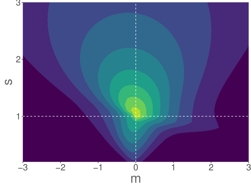
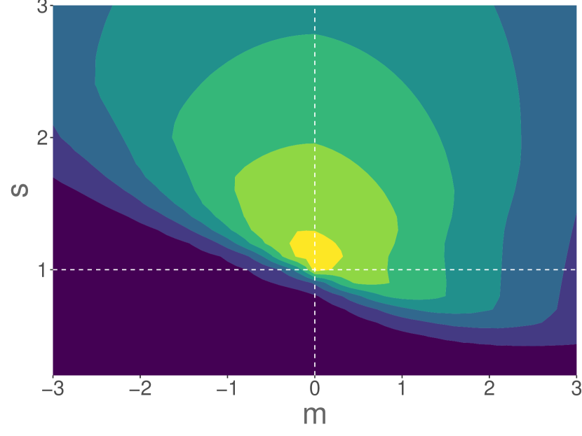
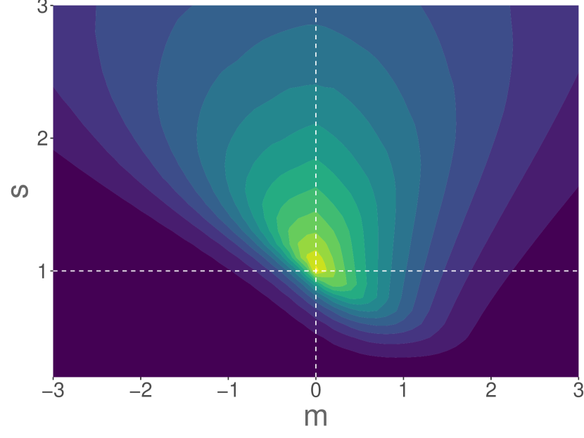
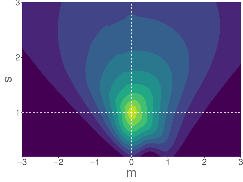
Here we consider the IMH algorithm with target distribution $\pi\sim\mathcal{N}(0,1)$ and proposal $\hat{J}\sim\mathcal{N}(m,s^{2})$ with hyperparameters $m\in\mathbb{R}$ and $s\in\mathbb{R}_{+}$. Our goal is to determine the values of the hyperparameters $m$ and $s$ that give rise to the IMH algorithm with fastest convergence. For this purpose, we adopt Tuning scheme 4, and obtain the optimal hyperparameter $(m_{*},s_{*})$ by

(29) $$(m_{*},s_{*})=\operatorname*{arg\,max}_{(m,s)\in\mathbb{R}\times\mathbb{R}_{+}}\ell_{(m,s)}(\mu).$$

As $\ell_{(m,s)}(\mu)$ we consider both lower bounds $\ell_{1,(m,s)}(\mu)$ from Proposition 3.3 and $\ell_{2,(m,s)}(\mu)$ from Proposition 3.4. We determine the optimal hyperparameter $(m_{*},s_{*})$ by solving 29 numerically $6$ times, by testing the following $6$ different probability measures:

• $\mu_{1}\sim\mathcal{N}(1,2^{2})$,

• $\mu_{2}\sim\text{Weib}(3,2)$,

• $\mu_{3}\sim\text{Unif}([0,1])$,

• $\mu_{4}\sim\frac{1}{2}\mathcal{N}(5,2^{2})+\frac{1}{2}\mathcal{N}(-3,1^{2})$,

• $\mu_{5}\sim\text{Exp}(1)$,

• $\mu_{6}\sim\text{Gamma}(3,2)$.

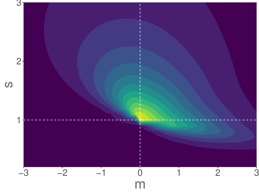
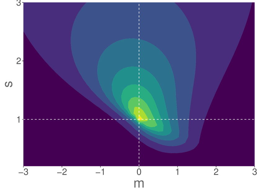
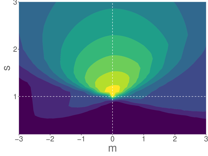
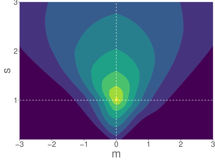
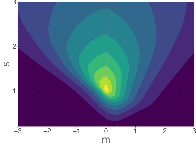
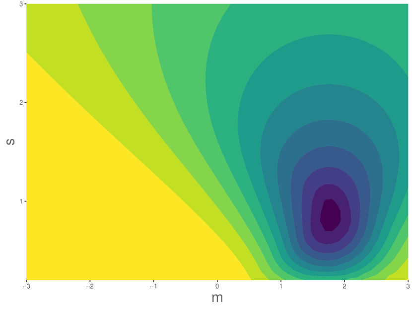
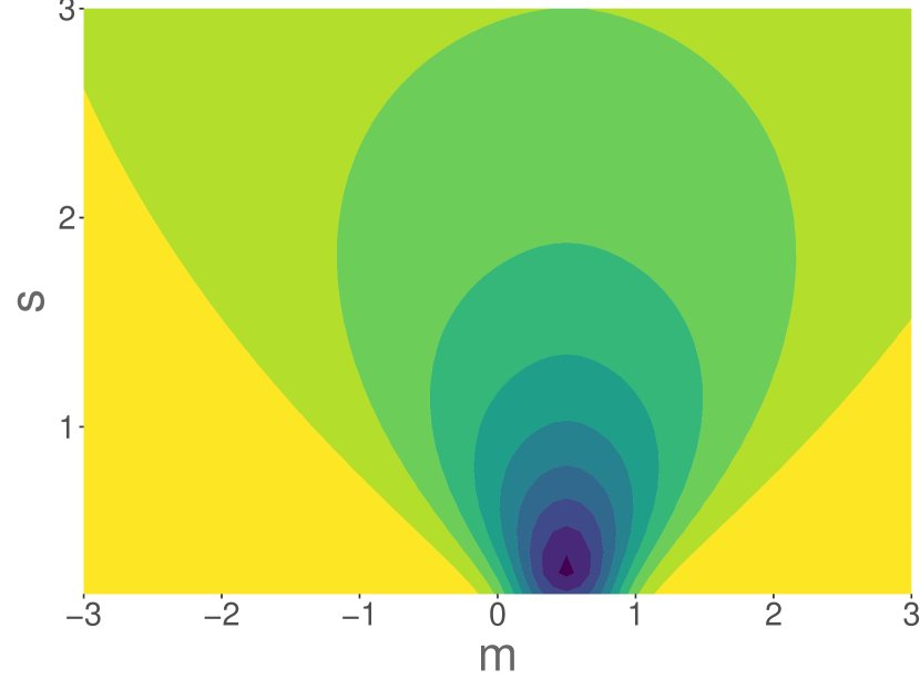
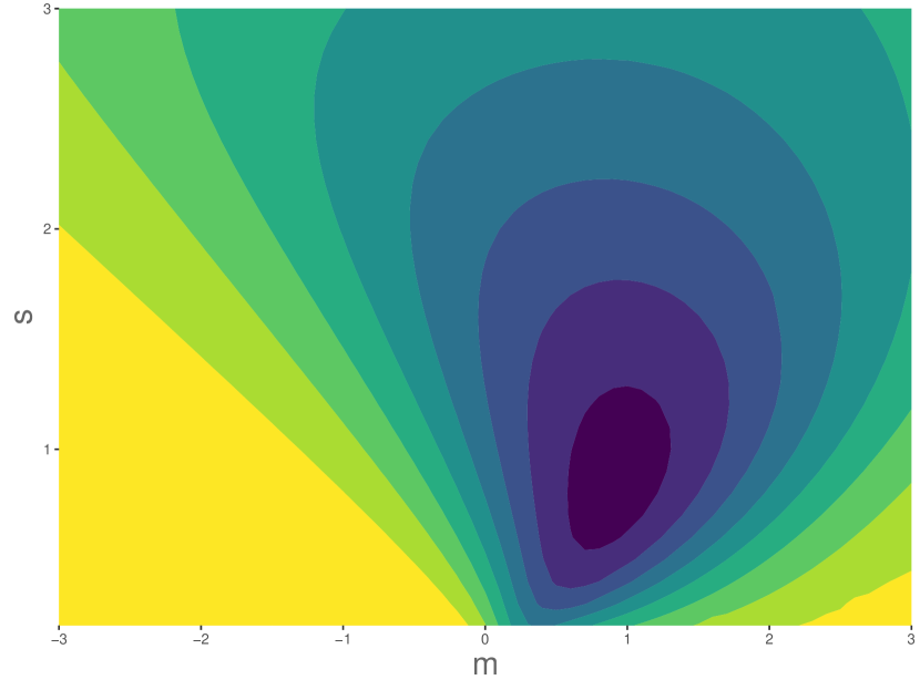
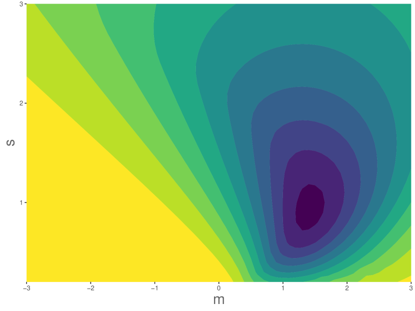
For all measures $\mu_{i},i=1,\dots,6$, we evaluated the lower bounds $\ell_{1,(m,s)}(\mu_{i})$ and $\ell_{2,(m,s)}(\mu_{i})$ for values $(m,s)$ in the rectangle $[-3,3]\times[0.2,3]$ (more specifically, on a grid with increments $0.1$ in both directions). Interestingly, for all $i=1,\dots,6$, the maximum value of either lower bounds was achieved in correspondence of $(m,s)=(0,1)$. In Figures 2 and 3 we plotted the contour plots of the lower bounds $\ell_{1,(m,s)}(\mu_{i})$ and $\ell_{2,(m,s)}(\mu_{i})$, respectively, for $i=1,\dots,6$, and $(m,s)\in[-3,3]\times[0.2,3]$, and indicated the maxima with dashed white lines.

This numerical results indicate that, among the independent proposal distributions $\hat{J}_{(m,s)}\sim\mathcal{N}(m,s^{2})$, the proposal that determines the IMH algorithm with fastest convergence to the target $\pi\sim\mathcal{N}(0,1)$ is $\hat{J}_{(0,1)}\sim\mathcal{N}(0,1)$. This result is not surprising. In fact, when $(m,s)=(0,1)$, the proposal has the same distribution as the target $\pi$. Consequently, the MH acceptance probability is $\min\left\{1,\frac{\pi(y)J(x|y)}{\pi(x)J(y|x)}\right\}=1$, i.e., all proposals are accepted. This means that when $\hat{J}=\pi$, the IMH algorithm is equivalent to sampling directly from the target, which is the fastest algorithm to sample from $\pi$.

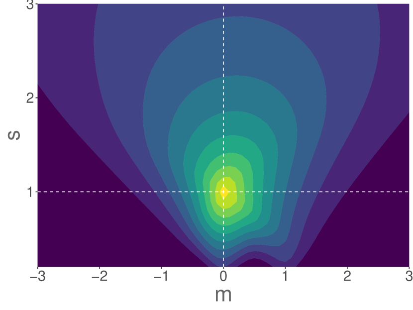
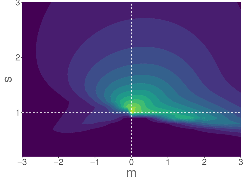
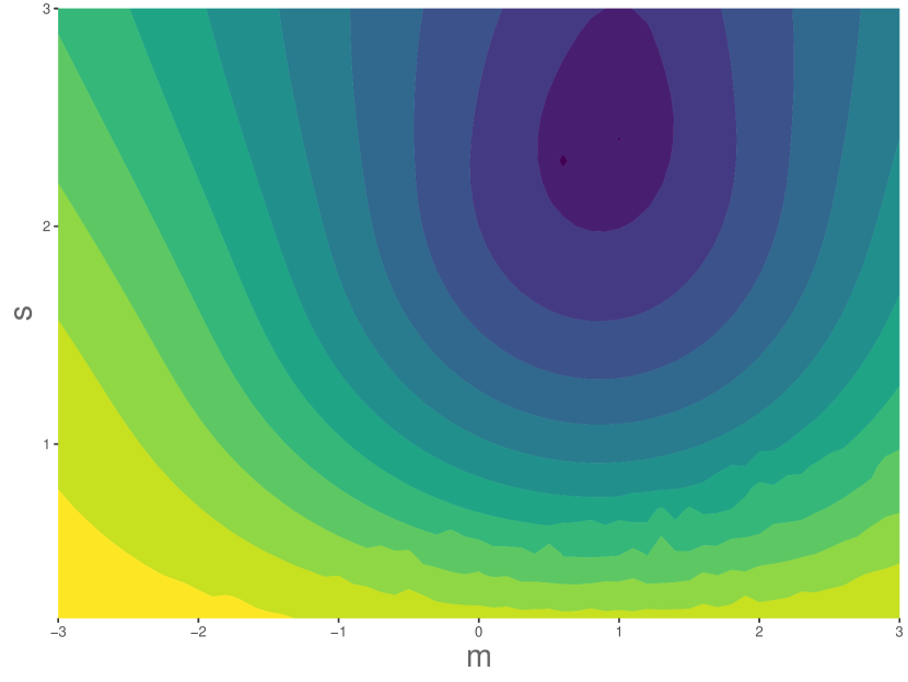
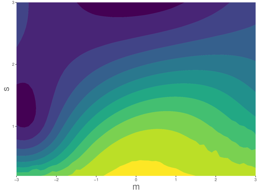
We also investigated the upper bounds obtained in Propositions 3.1 and 3.2. However, we did not identify any interesting pattern. In Figure 4 we show the contour plots of the upper bound from Proposition 3.2, for $i=1,\dots,6$, and $(m,s)\in[-3,3]\times[0.2,3]$. Nevertheless, upper bounds carry useful information. In fact, by means of both a lower and an upper bound we identify a closed interval containing the rate function, and therefore provide good quantitative estimates for the rate of convergence of the algorithm.

(a) $\mu_{1}\sim\mathcal{N}(1,2^{2})$

(b) $\mu_{2}\sim\text{Weib}(3,2)$

(c) $\mu_{3}\sim\text{Unif}([0,1])$

(d) $\mu_{4}\sim\frac{1}{2}(\mathcal{N}(5,2^{2})+\mathcal{N}(-3,1))$

(e) $\mu_{5}\sim\text{Exp}(1)$

(f) $\mu_{6}\sim\text{Gamma}(3,2)$

Figure 4. Contour plot of the upper bound from Proposition 3.2 as a function of $(m,s)$, for different choices of $\mu$. The $x$ and $y$ axes represent values of $m$ and $s$, respectively.

Acknowledgments

I would like to express my sincere gratitude to my advisor, Prof. Pierre Nyquist (Chalmers & Gothenburg University), for his dedicated mentorship and invaluable support in the development of this work.

This research was supported by the Swedish e-Science Research Centre (SeRC).

References

- [AG07] S. Asmussen and P.. Glynn “Stochastic simulation: algorithms and analysis” Springer, 2007
- [And+03] C. Andrieu, N. De Freitas, A. Doucet and M.. Jordan “An introduction to MCMC for machine learning” In Machine learning 50 Springer, 2003, pp. 5–43
- [And+22] C. Andrieu, A. Lee, S. Power and A.. Wang “Comparison of Markov chains via weak Poincaré inequalities with application to pseudo-marginal MCMC” In Ann. Statist. 50.6 Institute of Mathematical Statistics, 2022, pp. 3592–3618
- [And+23] C. Andrieu, A. Lee, S. Power and A.. Wang “Weak Poincaré Inequalities for Markov chains: theory and applications”, 2023 arXiv:2312.11689 [math.PR]
- [BD19] A. Budhiraja and P. Dupuis “Analysis and approximation of rare events” In Representations and Weak Convergence Methods. Series Prob. Theory and Stoch. Modelling 94 Springer, 2019
- [Bes94] J. Besag “Comments on “Representations of knowledge in complex systems” by U. Grenander and MI Miller” In J. Roy. Statist. Soc. Ser. B 56.591-592, 1994, pp. 4
- [Bie16] J. Bierkens “Non-reversible Metropolis-Hastings” In Stat. Comput. 26.6 Springer, 2016, pp. 1213–1228
- [BNS21] J. Bierkens, P. Nyquist and M.. Schlottke “Large deviations for the empirical measure of the zig-zag process” In Ann. Appl. Probab. 31.6 Institute of Mathematical Statistics, 2021, pp. 2811–2843
- [BR08] M. Bédard and J.. Rosenthal “Optimal scaling of Metropolis algorithms: Heading toward general target distributions” In Canad. J. Statist. 36.4 Wiley Online Library, 2008, pp. 483–503
- [DDN18] J.. Doll, P. Dupuis and P. Nyquist “A large deviations analysis of certain qualitative properties of parallel tempering and infinite swapping algorithms” In Appl. Math. Optim. 78 Springer, 2018, pp. 103–144
- [DHN00] P. Diaconis, S. Holmes and R.. Neal “Analysis of a nonreversible Markov chain sampler” In Ann. Appl. Probab. 10.3 Institute of Mathematical Statistics, 2000, pp. 726–752 DOI: 10.1214/aoap/1019487508
- [Dua+87] S. Duane, A.. Kennedy, B.. Pendleton and D. Roweth “Hybrid monte carlo” In Physics letters B 195.2 Elsevier, 1987, pp. 216–222
- [Dup+12] P. Dupuis, Y. Liu, N. Plattner and J.. Doll “On the infinite swapping limit for parallel tempering” In Multiscale Model. Simul. 10.3 SIAM, 2012, pp. 986–1022
- [DV75] M.. Donsker and S… Varadhan “Asymptotic evaluation of certain Markov process expectations for large time, I” In Commun. Pure Appl. Math. 28.1 Wiley Online Library, 1975, pp. 1–47
- [DV75a] M.. Donsker and S… Varadhan “Asymptotic evaluation of certain Markov process expectations for large time, II” In Comm. Pure Appl. Math. 28.2 Wiley Online Library, 1975, pp. 279–301
- [DV76] M.. Donsker and S… Varadhan “Asymptotic evaluation of certain Markov process expectations for large time, III” In Commun. Pure Appl. Math. 29.1 Wiley Online Library, 1976, pp. 398–461
- [DW22] P. Dupuis and Guo-Jhen Wu “Analysis and Optimization of Certain Parallel Monte Carlo Methods in the Low Temperature Limit” In Multiscale Model. Simul. 20.1, 2022, pp. 220–249
- [Fra+10] B. Franke, C.-R. Hwang, H.-M. Pai and S.-J. Sheu “The behavior of the spectral gap under growing drift” In Trans. Amer. Math. Soc. 362.3, 2010, pp. 1325–1350
- [Fri+93] A. Frigessi, P. Stefano, C.-R. Hwang and S.-J. Sheu “Convergence rates of the Gibbs sampler, the Metropolis algorithm and other single-site updating dynamics” In J. R. Stat. Soc. Ser. B. Stat. Methodol. 55.1 Oxford University Press, 1993, pp. 205–219
- [Has70] W.. Hastings “Monte Carlo sampling methods using Markov chains and their applications” Oxford University Press, 1970
- [HHS05] C.-R. Hwang, S.-Y. Hwang-Ma and S.-J. Sheu “Accelerating diffusions” In Ann. Appl. Probab. 15.2, 2005, pp. 1433–1444
- [Met+53] N. Metropolis et al. “Equation of state calculations by fast computing machines” In J. Chem. Phys. 21.6 American Institute of Physics, 1953, pp. 1087–1092
- [MN24] F. Milinanni and P. Nyquist “A large deviation principle for the empirical measures of Metropolis–Hastings chains” In Stochastic Processes and their Applications 170 Elsevier, 2024, pp. 104293
- [MN24a] F. Milinanni and P. Nyquist “On the large deviation principle for Metropolis-Hastings Markov Chains: the Lyapunov function condition and examples” In arXiv preprint arXiv:2403.08691, 2024
- [MT96] K.. Mengersen and R.. Tweedie “Rates of convergence of the Hastings and Metropolis algorithms” In Ann. Statist. 24.1 Institute of Mathematical Statistics, 1996, pp. 101–121
- [Pla+11] N. Plattner et al. “An infinite swapping approach to the rare-event sampling problem.” In J. Chem. Phys. 135.13, 2011, pp. 134111
- [Pow+24] S. Power, D. Rudolf, B. Sprungk and A.. Wang “Weak Poincaré inequality comparisons for ideal and hybrid slice sampling”, 2024 arXiv:2402.13678 [stat.CO]
- [RC04] C.. Robert and G. Casella “Monte Carlo Statistical Methods”, Springer Texts in Statistics New York, NY: Springer New York, 2004
- [Ros03] J.. Rosenthal “Asymptotic variance and convergence rates of nearly-periodic Markov chain Monte Carlo algorithms” In J. Amer. Statist. Assoc. 98.461 Taylor & Francis, 2003, pp. 169–177
- [RR98] G.. Roberts and J.. Rosenthal “Optimal scaling of discrete approximations to Langevin diffusions” In Journal of the Royal Statistical Society: Series B (Statistical Methodology) 60.1 Wiley Online Library, 1998, pp. 255–268
- [RS15] L. Rey-Bellet and K. Spiliopoulos “Irreversible Langevin samplers and variance reduction: a large deviations approach” In Nonlinearity 28.7 IOP Publishing, 2015, pp. 2081
- [RS15a] L. Rey-Bellet and K. Spiliopoulos “Variance reduction for irreversible Langevin samplers and diffusion on graphs” In Electron. Commun. Probab., 2015
- [RS16] L. Rey-Bellet and K. Spiliopoulos “Improving the convergence of reversible samplers” In J. Stat. Phys. 164 Springer, 2016, pp. 472–494
- [RT96] G.. Roberts and R.. Tweedie “Exponential convergence of Langevin distributions and their discrete approximations” In Bernoulli, 1996
- [SFR10] C. Sherlock, P. Fearnhead and G.. Roberts “The random walk Metropolis: linking theory and practice through a case study” In Statistical Science 25.2, 2010, pp. 172–190
- [Tie94] L. Tierney “Markov Chains for Exploring Posterior Distributions” In Ann. Statist. 22.4 Institute of Mathematical Statistics, 1994, pp. 1701–1728