Waveform Design of Multi-User-Multi-Target ISAC System based on Kullback–Leibler Divergence
Abstract
This paper presents a novel framework that leverages the Kullback-Leibler divergence (KLD) to analyze and optimize performance trade-offs in integrated sensing and communication (ISAC) systems. We consider a multiple-input-multiple-output (MIMO) base station that simultaneously serves communication user equipments (UEs) and detects multiple targets using shared antenna deployment. The proposed KLD-based approach provides a unified performance measure encompassing both UE error rate and target detection capability. We apply this approach on two well-known communication beamforming techniques, maximum ratio transmission (MRT) and zero-forcing (ZF), and evaluate the effect on the radar subsystem. Furthermore, two optimization problems are formulated and solved. The first one optimizes the KLD of the radar subsystem for given constraints on the communication KLD, whereas the second one focuses on communication waveform KLD-based optimization and constrained radar KLD. These optimization problems are solved using a projected gradient method with an adaptive penalty for the radar waveform and a gradient-assisted interior point method for the communication waveform. Through theoretical derivations and extensive simulations, it is demonstrated that our approach can be a powerful tool for characterizing and optimizing the performance trade-offs of ISAC under various configurations. The results also show significant improvements in both sensing and communication performance by the KLD-optimized system compared to well-known benchmarks, such as conventional MRT and ZF for the communication subsystem, and the conventional identity covariance design for the radar subsystem. These findings support the holistic design and optimization of ISAC in next-generation wireless networks.
Index Terms:
Integrated sensing and communication, multiple-input-multiple-output (MIMO), radar, zero-forcing, maximum ratio transmission (MRT), beamforming, optimization, Kullback–Leibler divergence (KLD).I Introduction
The rapid evolution of wireless communication networks, particularly with the advent of fifth-generation (5G) technology, has dramatically expanded the landscape of interconnected devices and services. This technological leap has enabled a wide array of applications that depend heavily on advanced sensing capabilities. From autonomous vehicles and unmanned aerial vehicles (UAVs) to the Internet-of-Things (IoT) ecosystems, these applications are pushing the boundaries of traditional communication systems, necessitating the integration of sophisticated sensing functionalities [1, 2, 3, 4]. As we stand on the threshold of the sixth-generation (6G) era, network operators and service providers face unprecedented challenges in not only delivering robust communication services but also in integrating advanced sensing-based applications such as detection, localization, tracking, navigation, and environmental surveillance [5, 6, 7].
Integrated Sensing and Communications (ISAC) systems have garnered significant interest in the research and industrial communities to meet these emerging demands. ISAC systems aim to synergistically merge sensing and communication functionalities within the same infrastructure, thereby optimizing the use of available resources at base stations (BSs) for dual purposes [8, 9, 10, 11, 12, 13]. This integration can be achieved through various architectural approaches. For example, in a separated deployment, the BS antennas are allocated distinctly between communication and radar subsystems, which can simplify the system design but may underutilize resources. In contrast, the shared deployment strategy employs all antennas for both functionalities, potentially offering higher resource efficiency at the cost of the increased complexity and the need for more sophisticated signal processing techniques[14, 15].
The evolution of ISAC systems has been accelerated by the advances in multi-antenna technologies, particularly massive Multiple-Input Multiple-Output (MIMO) systems. These systems allow for the generation of highly directional beams and support simultaneous service to a large number of users, thereby significantly enhancing both communication capacity and sensing accuracy, usually done by exploiting spatial diversity by setting the antenna separation to a minimum of half wavelength [16]. The synergy between ISAC and massive MIMO presents a promising avenue for meeting the stringent requirements of future wireless networks. However, evaluating the performance of ISAC systems poses unique challenges due to their dual functionality. Traditionally, communication and sensing subsystems have been assessed using distinct metrics, with communication performance measured by achievable rate, outage probability, and bit error rate, while the sensing performance is typically evaluated using metrics like estimation rate, detection probability, false alarm probability, and mean square error (MSE) [17]. This disparity complicates the holistic assessment and optimization of ISAC systems.
I-A Literature review
To address these challenges mentioned above, there has been a growing interest in developing unified performance measures that can simultaneously capture both sensing and communication capabilities. One such measure that has gained traction is the Kullback-Leibler divergence (KLD), also known as the relative entropy. KLD has a well-established history in information theory and has been extensively used in the analysis and design of sensing systems, particularly in the context of MIMO radars [18, 19, 20]. It quantifies the dissimilarity between two probability distributions, serving as a measure of the information gain achieved by using one distribution over another. While the application of KLD in sensing systems is well-established, its potential in characterizing communication system performance remains open. Recent studies have begun to bridge this gap, demonstrating the utility of KLD in assessing the performance trade-offs between sensing and communication functionalities in ISAC systems. For instance, in our previous works [21, 22], we employed KLD to analyze performance in systems with separated antenna deployment, while in [23] we proposed a low-complexity unified objective function based on KLD, aimed at optimizing network resources for both separated and shared deployment scenarios. Moreover, further insights about the achievable KLD trade-off in ISAC systems is explored in [24], and more designs have been discovered. Nonetheless, the literature lacks a comprehensive investigation and beamforming design for a generalized multi-user-multi-target (MUMT) ISAC system using the promising KLD.
Further efforts have explored various optimization approaches for ISAC systems, each addressing specific aspects of system performance. For example, joint radar-communication beamforming optimization based on the Cramér-Rao Bound (CRB) has been proposed to improve both sensing and communication performance [25]. This approach minimizes the CRB of angle estimation for radar while maximizing the signal-to-interference-plus-noise ratio (SINR) for communication, thus enhancing the accuracy of sensing and the quality of communication simultaneously. However, these methods often focus on optimizing individual components rather than adopting a unified framework that captures the interplay between different functionalities. Beamforming optimization has been a particular focus, with studies investigating partially connected hybrid beamforming designs to address the hardware complexity of fully digital systems [26]. While these approaches offer practical advantages in terms of implementation, they do not fully capture the nuanced trade-offs between sensing and communication performance, especially in scenarios where these functionalities are deeply integrated. Waveform optimization has also been extensively studied, with recent work proposing a symbol-level precoding scheme using a faster-than-Nyquist approach to enhance the spectral efficiency in bandwidth-constrained environments [27]. This approach focuses on communication waveform design while considering the radar functionality as a constraint, ensuring that the designed waveforms maintain certain radar performance metrics. However, this work does not consider a unified optimization framework that could simultaneously address the needs of both radar and communication subsystems.
I-B Motivation and contribution
Despite these advances, current approaches often fall short of fully exploiting the potential of integrated systems. Most notably, there is a need for more comprehensive models that can accurately reflect the real-world operation of ISAC systems, particularly in scenarios where communication signals can be utilized for radar target detection alongside dedicated radar signals. Exploiting the interference from communication signals as a source of information for radar operations enhances radar detection capabilities and maximises the system’s overall resource efficiency [14]. This dual-use of communication signals represents a significant departure from traditional approaches, which typically treat interference as a detrimental factor to be mitigated rather than leveraged[28, 29].
Toward these objectives and motivated by the fact that KLD is able to provide a unified measure for ISAC system holistically, this paper proposes a novel framework based on the Kullback-Leibler divergence (KLD) to characterize and optimize the sensing-communication performance trade-offs in shared antenna deployment ISAC systems. This work addresses several gaps in the existing literature by introducing a unified KLD-based performance measure that captures the synergies and trade-offs between sensing and communication in ISAC systems. By considering the shared deployment scenario and proposing specific optimization techniques for both radar and communication waveforms, we provide a comprehensive approach for system optimization that reflects the true potential of ISAC systems in future wireless networks. Additionally, our analysis of different beamforming techniques within this framework offers valuable guidance for designing ISAC systems that can effectively balance the needs of both radar and communication functionalities. Our system model consists of a multiple-input-multiple-output (MIMO) base station (BS) that simultaneously serves communication user equipment (UEs) and detects multiple targets using shared resources. The key contributions of our work are as follows:
-
•
Unified Performance Measure: We derive the Kullback-Leibler Divergence (KLD) specifically for the integrated operation of communication and radar systems within ISAC. This performance measure unifies the communication error rate with radar target detection capabilities into a single objective function. By deriving this KLD-based metric for communication and radar components, we optimise ISAC system design holistically, addressing the trade-offs and enhancing overall system performance.
-
•
Inherent Exploitation of Communication Interference: Our framework accounts for the fact that communication signals can also be exploited for radar target detection alongside dedicated radar signals, providing a more comprehensive and useful model of ISAC system operation. This dual-use approach enhances the radar performance by utilizing communication interference as an additional source of information for target detection.
-
•
KLD-based Optimized ISAC: We propose two novel optimization techniques: radar and communication waveform KLD-based optimization. Both maximize their respective KLD measures subject to the minimum KLD of both subsystems and power constraints. The non-convex radar optimization employs a projected gradient method with an adaptive penalty, while the communication optimization uses a gradient-assisted interior point method. These techniques efficiently handle ISAC waveform design’s complex, multi-dimensional nature, enabling balanced performance optimization across both subsystems within system constraints.
-
•
Benchmark Analysis: We investigate two benchmark beamforming techniques for the communication subsystem, namely maximum ratio transmission (MRT) and zero-forcing (ZF), and analyze their impact on the overall system performance within our KLD-based framework. This analysis provides practical insights for system designers seeking to optimize ISAC performance in shared deployment scenarios with a complexity-performance trade-off.
Our results demonstrate that the proposed KLD-based optimization techniques significantly enhance ISAC system performance compared to the MRT and ZF scenarios for the communication subsystem and the radar subsystem’s conventional identity covariance design. The radar waveform optimization shows substantial improvements in both target detection and communication performance, while the communication waveform optimization primarily benefits the communication subsystem with modest radar performance gains. Both techniques exhibit robust performance across varying SNR levels, with the radar optimization demonstrating particularly stable computational efficiency. Notably, incorporating communication signals in radar detection significantly enhances overall system performance, especially in scenarios with limited dedicated radar resources. These findings provide valuable insights for designing efficient shared deployment ISAC systems that balance sensing and communication requirements.
I-C Paper organization
The paper is structured as follows. Section II presents the system model. Sections III and IV analyze the communication and radar systems, respectively, including the derivations of KLD for each system. In Section V, the first KLD-based optimisation technique considers the radar KLD sum under communication KLD constraint is investigated. Section VI introduces the second KLD-based optimisation technique based on communication KLD sum with radar KLD constraint. Section VII displays the numerical results, and finally, Section VIII concludes the work.
: Bold uppercase letters (e.g., ) denote matrices, and bold lowercase letters (e.g., ) denote vectors. Superscripts , , and , denote the conjugate, transpose, and Hermitian transpose, respectively. Subscripts and relate to the communication, and radar subsystems, respectively.
II System Model
This paper is concerned in an ISAC system that comprises an antenna MIMO-BS. The antennas are utilised for detecting a maximum number of targets and serving number of single-antenna communication user equipments (UEs) in the downlink direction using the shared deployment scenario. The total transmitted power available at BS is which is utilised for both sensing and data communication duties. The portions of the power that are allocated to the radar and communication subsystems are respectively denoted as and , where . As a starting point, non-optimised beamforming techniques such as MRT and ZF are employed at BS to precode the information of communication UEs [16]. These techniques serve as benchmarks for our subsequent optimized systems, which will be introduced and analyzed later in Sections V and VI. The combined transmitted ISAC signal will be as follows,
| (1) |
where is a vector of communication UEs symbols, is a vector of the baseband radar waveforms for the potential targets, represents the precoding matrix for the communication subsystem, and represents the precoding matrix for the radar subsystem. Notably, the transmitted signals vector is transmitted from the BS and received at the UEs as well as the targets which reflect the received version of back to the BS. Although the radar signal component received at the UEs might impose interference that cannot be eliminated by the users, the communication signal component received at the targets and reflected back to the BS carries information about the target. Therefore, by carefully designing the precoding matrices at the BS, the sensing information can be enhanced by exploiting the communication signal for sensing targets as well. This dual-use approach enhances radar performance by utilizing the communication signal as an additional source of information. Moreover, the radar waveform design in our work is based on the combined transmit signal covariance matrix for the -th beam such that the covariance matrix of the -th transmit beam is , where , and is the total number of snapshots. This formulation allows us to incorporate the communication signals into the radar detection process. It should be noticed that the power for the radar is integrated into the precoding vector , where it is designed to have , and , where is the th beam precoding vector, and is the Frobenius norm.
II-A Communication System
At each instance, a data symbol intended for the -th UE is drawn from a certain normalised constellation, i.e, . The received signal at the -th UE can be formulated as follows,
| (2) |
where represents the channel from the BS to the -th UE, represents the IUI on the -th UE from the other UEs, the variable is the channel pathloss from BS to the -th UE with represents the distance from BS to the -th UE, and is the pathloss exponent, and id the interference-plus-noise term with representing the additive white Gaussian noise (AWGN). The precoding vector for the communication system is , which is typically designed based on the given channel matrix from MIMO-BS to UEs , where the elements of are independent and identically distributed (i.i.d) complex Gaussian random variables with zero mean and variance . In the next two subsections, we revisit the conventional MRT and ZF designs which are typically used to precode the communication data symbols at the BS. These precoding schemes will serve as benchmarks for our designs.
II-A1 MRT beamforming
In MRT precoding, the amount of received power at the UEs is maximized without taking into account the imposed interference. This approach usually lead to acceptable performance at low SNR values but its performance deteriorates at large SNRs. The normalized MRT beamforming matrix is designed for all UEs based on the channel matrix as follows,
| (3) |
where is the power allocation matrix for the communication users, which is a diagonal matrix that controls the power allocated for each UE.
II-A2 ZF beamforming
On the contrary, ZF precoding eliminates inter-user interference (IUI) at the UEs regardless of the amount of the received power. This approach usually results in excellent performance at high SNR values. The normalized ZF beamforming matrix is designed also based on the channel matrix, and can be represented as follows,
| (4) |
where is the ZF beamformer before normalisation.
II-B Radar system
The radar system proposed in this study is designed for high adaptability, allowing for real-time adjustments in detection capabilities on a per-frame basis, where each frame is composed of snapshots. A key parameter of this system is , representing the count of radar beams emitted during a specific detection frame. By harnessing MIMO radar technology, multiple beams can be generated simultaneously using orthogonal signals [30, 31]. Consequently, signifies the upper limit of detectable targets within a single frame.
This radar system’s design is robust, as it can explore multiple angular-range-Doppler bins over successive frames, thereby increasing the chance of identifying more targets. Furthermore, its flexibility in varying the number of emitted beams allows for the simultaneous detection of a larger set of targets, providing the ability to fine-tune the system’s detection capability according to different operational demands. However, it is crucial to acknowledge that the value of is naturally constrained by the available number of antennas and the total number of UEs being serviced by the BS, highlighting the critical need for efficient waveform design, and resource allocation strategies in ISAC systems.
Our focus aligns with scenarios where targets are spatially separated, ensuring each target is confined to a distinct radar bin, as explored in prior studies [32, 33]. Additionally, the literature offers a range of algorithms developed to separate signals from closely spaced or unresolved targets, facilitating accurate target enumeration [34]. A straightforward method to count detected targets involves applying the detection mechanism across all radar bins spanning the angular, range, and Doppler dimensions. The total radar return signal at the -th snapshot is shown as follows,
| (5) |
where is the target response matrix of the BS-Target-BS route for the -th target, following a Rayleigh distribution [35]. The is the additive white Gaussian noise vector at the -th snapshot. To analyze the radar returns from all beams, a series of matched filters are typically applied, each tuned to a specific waveform , which corresponds to a particular radar angular-range-Doppler bin. Because is orthogonal to for all , the radar returns from distinct beams can be effectively separated, enabling independent detection of each potential target. The radar precoding matrix is designed such that the covariance matrix is . The received signal for the -th target at the BS, under the binary hypotheses , where signifies target presence and denotes target absence, can be mathematically represented as follows,
| (6) |
The is the additive white Gaussian noise vector at the -th snapshot.
III The KLD of communication system: ZF and MRT precoding
In this section, we derive the KLD of the communication system for two typical scenarios, namely, the MRT, and the ZF beamforming schemes using the shared deployment antenna configuration. The analysis is carried out for the normalized precoders introduced in Section II-A.
In order to, derive the KLD, it is necessary to establish the statistical properties of the signal, IUI, radar interference, and noise components. For a pair of multivariate Gaussian distributed random variables having mean vectors of and and covariance matrices of and , the KLD can be derived as,
| (7) |
The application of this formula to the communication system requires the determination of the mean vectors and covariance matrices for each precoding scheme.
III-A MRT beamforming
For the MRT precoding scheme, the analysis encompasses the desired signal, IUI, radar interference, and noise components. The examination starts with the IUI term, which is the second term in (2), which can be written as,
| (8) |
Since that the elements of and are i.i.d. complex Gaussian random variables with zero mean and variance , the term is the inner product of two independent complex Gaussian vectors. Therefore, central limit theorem (CLT) can be invoked to show that the distribution of tends to be complex Gaussian with zero mean and variance for a significant number of antennas . On the other hand, the normalization term follows a chi-squared distribution with degrees of freedom, scaled by . Consequently, the exact distribution of is a ratio of complex normal variables to the square root of a chi-squared variable. Unfortunately, this ratio distribution does not have a simple closed-form expression. However, it is worth noting that we can approximate its behavior for large and , by using the law of large numbers, . Consequently, using this approximation, we can write (8) as,
| (9) |
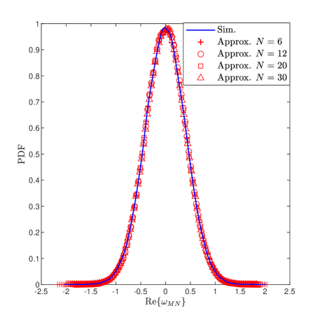
Now, is a sum of independent complex normal variables. By invoking the CLT, for large , this sum approaches a complex normal distribution with zero mean and a variance of,
| (10) |
The accuracy of this approximated density of is validated by simulation and shown in Fig.1, which compares it with simulated density functions under different values of . It can be also shown that the distribution of can be well approximated by a complex Gaussian distribution using the CLT, particularly for large . This approximation yields a mean of , and a variance of,
| (11) |
where . Now, the equivalent IUI and radar interference plus noise term can be approximated as a complex Gaussian random variable with zero mean and variance . In order to find the KLD for the MRT case with matrix normalization, we need to evaluate the expected value of the desired signal power, which is represented by the first term in (2). This term, can be expressed as follows,
| (12) |
The expected value of this term can be approximated using the properties of the chi-squared distribution and the approximation for a random variable ,
| (13) |
After deriving the statistical properties of the signal and interference components, the KLD formula can be applied. Given that , and , and , these can be substituted into equation (7), then the KLD can be found as [21, Corollary 1],
| (14) |
where which depends on the transmitted data constellation, and thus is constant for a given constellation, for example, for MPSK signalling, . Finally, substituting (13) in (14), then the KLD for MRT precoding with matrix normalization can be found as,
| (15) |
III-B ZF beamforming
With ZF precoding, the received signal at the -th user can be rewritten as follows,
| (16) |
where is the -th column of the normalized ZF precoding matrix. It should be noticed that the term as the ZF precoder completely eliminates the IUI. The mean vectors and covariance matrices for the -th and -th symbols are shown as follows,
| (17) | ||||
| (18) |
where due to the normalization of the ZF precoding matrix. Since , under flat fading channel, it can be shown that follows a Gamma distribution with shape parameter and scale parameter , denoted as , where . Let . By substituting (17), and (18) in (7), then the KLD can be reduced to,
| (19) |
where the expectation of can be calculated using the PDF of Gamma distribution as follows,
| (20) | ||||
Substituting this result into the expression for in (19), the final expression for the average KLD in the case of ZF precoder with matrix normalization can be reduced to,
| (21) |
III-C Conditional KLD for an Arbitrary Precoding Matrix and Given Channel Matrix
A conditional KLD for communication, in terms of the bamforming matrix and for a given channel matrix , is required to formulate an optimization problem for which can be designed based on the channel side information matrix. Accordingly, by considering the received signal representation in (2), the conditional mean vectors and variance can be obtained as follows,
| (22) |
| (23) |
where the assumptions of zero-mean, temporal whiteness, and wide-sense stationarity of the communication and radar signals, as well as their mutual orthogonality, have been utilized, it is important noting that the variance of the received signal for a given pair of symbols is equal. Therefore, the covariance is,
| (24) |
Substituting the mean vectors and covariance matrices from (22), and (24) into the KLD expression given in (7), we can obtain the KLD for the -th UE in communication subsystem for each possible pair of unequal data symbols , , this is done as follows,
| (25) |
where and , substituting it in the KLD expression which becomes,
| (26) |
It should be noted that the second term in this equation, represents the form of the SINR, where the interference is the sum of IUI and radar interference.
IV Radar system analysis
IV-A Composite detection and response matrix estimation
The main objective for typical radar systems is to detect targets and estimate the matrix response associated with each one. After separating different signals associated with different targets, such problem can be formulated for each target as a composite detection-estimation problem as follows,
| (27) |
This joint optimization problem aims to simultaneously detect the presence of a target (determining ) and estimate its response matrix () if present. Now, considering the hypotheses and , the PDF of the received signals vector under each of these hypotheses can be shown as a multivariate normal density, which can be written as
| (28) |
where , and . The generalized likelihood ratio test (GLRT) for the -th target is used to determine target existence or absence by comparing the likelihoods under the two hypotheses. The GLRT is derived as follows,
| (29) |
However, the PDF does not depend on under . Therefore, the target response matrix is typically estimated under , thus by using the maximum likelihood estimation theorem we obtain
| (30) |
Since the noise is Gaussian and the is normally distributed, the likelihood function is Gaussian, and the maximization leads to the least squares solution. Therefore, this maximization reduces to the following form,
| (31) |
This least squares solution provides an unbiased estimate of . Substituting the PDF in (28) into the GLRT, we obtain the following,
| (32) |
where and is the detection threshold that is a design parameter, for example, according to Neyman-Pearson lemma it can be determined to obtain a certain false alarm rate. Taking the logarithm and rearranging terms, we obtain the following expression, which now clearly includes the estimated target response matrix ,
| (33) |
The terms and are constant with respect to , so they can be absorbed into the threshold, which further simplifies our GLRT as follows,
| (34) |
where . This final expression correctly reflects the comparison between the hypotheses and , incorporating the estimated target response matrix in the covariance matrix . In order to utilize the whole snapshots whose received signals are independent, we average as follows,
| (35) |
where is the detection threshold that accounts for all snapshots and could be designed according to the Neyman-Pearson lemma as illustrated above.
IV-B The KLD of radar system
As the number of snapshots approaches infinity, the law of large numbers ensures that the estimated target response matrix converges in probability to the true value, i.e., . Assuming a large enough number of snapshots , this asymptotic behaviour allows us to treat as equivalent to in our subsequent analysis, simplifying our derivations while maintaining theoretical validity. Under this assumption, we can proceed with a more tractable derivation of the KLD for the radar subsystem.
V Radar Waveform Optimisation
Here, the radar waveform is optimised while using the ZF beamforming scheme for the communication subsystem. The optimisation problem can be shown as follows,
| (37a) | ||||
| s.t. | (37b) | |||
| (37c) | ||||
| (37d) | ||||
| (37e) | ||||
where is defined in (36). After substituting (36) in (37a), can be written as that is given on page V. This optimization problem focuses on the radar waveform while considering the whole ISAC system performance. The constraint on radar power (37d) is explicit because the radar waveform is our primary optimization variable. The communication power is implicitly considered through the ZF beamforming scheme and the constraint (37c) on communication performance. While the communication power is not directly optimized, it is indirectly influenced by the radar power allocation. Specifically, the communication subsystem utilizes its allocated power through the ZF beamforming scheme to distribute power to each UE, with weights predetermined based on the channel state information. This approach allows us to focus on the interplay between subsystems which is mainly governed by waveform design and interference management while maintaining system-wide performance.
To Tackle the optimisation problem in (38), we utilize the Projected Gradient method with a penalty function [36]. This method is chosen for its suitability to the non-linear, non-convex optimization problem [37]. This approach incorporates complex KLD constraints via the penalty function, while efficiently handles the radar power constraint through projection. It offers a balance between the solution quality and the computational efficiency, crucial for potential real-time ISAC applications. The method’s scalability with problem dimensionality further justifies the selection of this method for the radar waveform optimization task in the ISAC setup illustrated in the problem formulation. The optimization variable is a three-dimensional tensor, where , , and are all parts of this tensor. We define the objective function and a penalty function to handle the constraints in (37b) and (37c),
| (39) |
| (40) |
The gradient of the objective function, , is a gradient tensor computed element-wise, as detailed in Appendix I.A. The final equation is given by,
| (41) |
The gradient of the penalty function is also a gradient tensor, computed as,
| (42) |
where and with represents the indicator function. The gradients of and with respect to and , respectively, are provided in Appendix I.A. The final forms are given by,
| (43) | ||||
| (44) |
The update rule for the projected gradient method with penalty ensures that each iteration moves the solution towards optimality while maintaining feasibility, and can be shown as follows,
| (45) |
where is the gradient direction, combining the objective function gradient and the penalty function gradient, is the penalty parameter, which balances the importance of the objective function and the constraint satisfaction, is the step size, and is the projection onto the feasible set defined by the power constraint, ensuring that the power constraint in (37d) is always satisfied. The projection mechanism is shown in the following equation,
| (46) |
The step size is determined using a backtracking line search to ensure convergence. We find the smallest non-negative integer such that,
| (47) |
where . This condition, known as the Armijo condition, ensures a sufficient decrease in the penalized objective function [38]. The step size is then set as , where is a reduction factor. The penalty parameter is updated as follows,
| (48) |
where is a constant factor. This adaptive scheme increases the penalty when constraints are violated and keeps it constant when they are satisfied.
Algorithm 1 implements the projected gradient method with penalty for the radar waveform optimization problem. It iteratively updates the waveform by moving in the direction of the total gradient , which combines the gradients of the objective function gradient and the penalty function. The projection operator ensures that the power constraint is always satisfied. This projection is crucial as it maintains the feasibility of the solution with respect to the power constraint throughout the optimization process. The backtracking line search procedure is used to determine an appropriate step size at each iteration. This adaptive step size selection helps to ensure a sufficient increase in the objective function while maintaining the stability of the algorithm. The line search condition can be expressed as,
| (49) |
where is the penalized objective function. The penalty parameter is updated adaptively based on the constraint violation. This adaptive scheme allows the algorithm to balance between optimizing the objective function and satisfying the constraints. As the optimization progresses, if constraints are consistently violated, the increasing penalty parameter will put more emphasis on constraint satisfaction.
VI Communication optimisation
The communication subsystem optimization employs the gradient-assisted interior point method [39], contrasting with the projected gradient method with penalty used for radar optimization, due to the fundamental difference in optimization variable structure. While radar optimization involves a three-dimensional tensor , communication beamforming optimizes over a two-dimensional matrix . This reduced dimensionality makes IPM particularly suitable, potentially offering faster convergence and more precise solutions for the matrix optimization problem. The communication waveform is optimised while using conventional identity covariance matrix design for the radar subsystem with a covariance matrix set to . The optimisation problem can be shown as follows,
| (50a) | ||||
| s.t. | (50b) | |||
| (50c) | ||||
| (50d) | ||||
| (50e) | ||||
It is important to note that the radar power is uniformly distributed among the potential targets, as the radar covariance matrix ensures an omnidirectional beam flow. To solve this optimization problem, we need to derive the gradient of the objective function and the constraints. Let’s define the objective function as,
| (51) |
Now, to compute the gradient of the objective function, we need to derive the gradients of each objective function components.Let . Using the chain rule and the properties of matrix derivatives, the gradients can be expressed as,
| (52) | ||||
| (53) |
where , and . Finally, we can express the gradient of the objective function as,
| (54) |
Next, we need to consider the constraints of our optimization problem. The power constraint is given by,
| (55) |
The gradient of this constraint is derived straightforwardly as follows,
| (56) |
The gradient of the radar KLD constraint with respect to is derived as follows,
| (57) |
Solving the optimization problem defined in equations (50a)-(50d) involves employing the Interior Point Method (IPM) as outlined in Algorithm 2. This method efficiently handles constrained optimization using key parameters: an initial barrier parameter , a barrier reduction factor , and a convergence tolerance . The algorithm iteratively computes the objective function, constraints, and their gradients, checks the Karush-Kuhn-Tucker (KKT) conditions, and updates the solution using a Newton system and line search. The barrier parameter is reduced as in each iteration, gradually enforcing constraints more strictly. This process continues until or the maximum iterations are reached, yielding the optimal beamforming matrix that maximizes average communication KLD while satisfying radar and power constraints.
VII Numerical Results
In this section, we present the simulation results for both our conventional benchmarks and the two optimisation techniques introduced previously. The total transmit power is fixed at , and QPSK modulation is used throughout this section. The total number of antennas at BS is , a number of snapshots, the maximum number of potential radar targets is , and the number of UEs is . The pathloss exponent is to model the effect of large-scale fading, and the distances from the BS to the UEs are meters, respectively, and to the targets are meters, respectively. The channel variance is .
VII-A Trade-off for the conventional benchmarks
The conventional identity covariance matrix design is used for the radar subsystem with a covariance matrix is set to , whereas the communication subsystem uses MRT and ZF precoding introduced earlier.
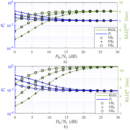
Fig. 2 presents the performance of the communication subsystem for both ZF and MRT beamforming schemes. In Fig. 2.a, the MRT scheme’s performance is depicted, with the KLD performance on the right -axis and the BER performance on the left. As can be observed from the figure, the KLD values for all UEs increase with until around dB, where a noticeable upper-bound occurs primarily caused by radar interference, with IUI contributing to a less extent. Similarly, the BER decreases with , indicating an improvement in the communication subsystem performance, but also exhibits the same error floor at around dB. Fig. 2.b illustrates the ZF scheme’s performance, exhibiting similar trends in the KLD and BER curves. However, compared to the MRT scheme, the ZF scheme shows an increase in KLD values and a decrease in BER values for the same received SNR, indicating that the primary source of interference is indeed caused by radar interference as IUI is cancelled using ZF precoding. Consequently, both the ZF and MRT schemes exhibit a drastic error floor in BER, or equivalently an upper bound for KLD, due to the unmitigated radar interference at . Moreover, this figure clearly shows the effectiveness of using KLD to characterize the communication system.
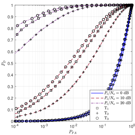
Fig. 3 shows the receiver operating characteristic (ROC) curves depicting the performance of the radar subsystem for the three potential targets across different scenarios, for the same ISAC system in Fig. 2 with ZF precoding for communication subsystem assumed. The ROC curves are obtained by plotting the probability of detection () versus the probability of false alarm () for each target. In Fig. 3, where dB, the ROC curves for all three targets , , and are relatively close to each other, indicating similar detection performance at low signal-to-noise ratios. In Fig. 3, with dB, the ROC curves for the three targets start to diverge, where exhibits the best performance, followed by followed by . This suggests that as the signal-to-noise ratio increases, the radar subsystem’s ability to detect the targets and distinguish between them improves. Finally, in Fig. 3, in which dB, the separation between the ROC curves becomes even more pronounced. As can be observed in 3, at , is for , , and , respectively, where maintains its superior performance, while and show significant improvements in their detection probabilities compared to the lower scenarios. This demonstrates that at high signal-to-noise ratios, the radar subsystem can effectively detect and differentiate between the three targets, with being the most easily detectable as it is the closest target to the BS.
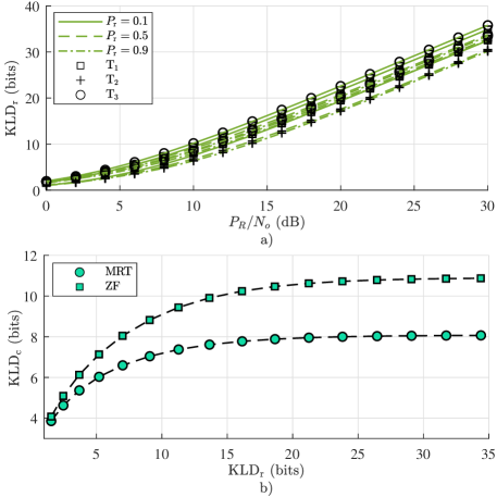
In Fig.4.a, the performance of the radar subsystem is illustrated through the achievable of each target versus the across different values of . It is shown that as increases, the achievable for each target also increases for all values of . This indicates that the radar subsystem’s performance improves with higher . The performance curves for different values are relatively close to each other, suggesting that the system’s performance is less sensitive to changes in because the communication subsystem signal is also incorporated in the target detection, using our improved system model.
Fig. 4.b presents the trade-off performance between radar and communication subsystems using the ZF and MRT for the communication subsystem and the conventional identity covariance design for the radar subsystem. The plot shows versus at equal power allocation between both subsystems, with each point on the curve representing a different value. The outperforms the slightly, as both of them exhibits saturation at higher due to the destructive interference from the radar subsystem mainly, while the shows a steady increase when moving from left to right on the curve. It can be observed from the figure that a of 8 bits can be achieved at dB for , whereas the same amount of is achieved at around dB, which implies an SNR gain of about dB in favour of ZF.
VII-B Radar Waveform KLD-based Optimisation
The radar waveform KLD-based optimization algorithm is configured with a maximum iteration limit of and a convergence tolerance of . The penalty parameter is initialized at , with a penalty increase parameter of , and an initial step size of . The KLD lower bounds and for all targets and UEs are set to 10 bits.
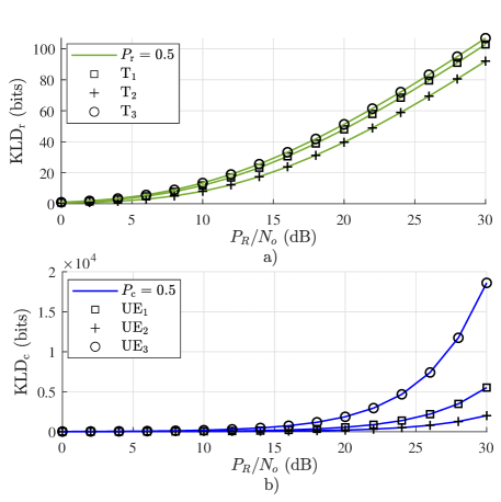
Fig. 5 illustrates the performance of the radar and communication subsystems using the optimized radar waveform. Fig. 5.a shows the achievable for each target as a function of . As can be seen from the figure, as increases, improves for all targets, indicating enhanced radar performance at higher power-to-noise ratios. It can be also observed that target T3 consistently achieves the highest , followed by T1 and T2, reflecting their respective distances from the BS. At dB, the values are approximately bits for T1, T2, and T3 respectively. These values increase to about bits at dB, showing improvement in radar performance. The rate of improvement after 15 dB appears to enter a near-linear relationship with , suggesting a consistent pattern of performance enhancement in the radar system.
Fig. 5.b depicts the communication subsystem performance through versus . The for values between - dB exhibits a minimal improvement, indicative of system infeasibility in this low power regime. This minimal growth at the low SNR region is attributed to the system’s inability to meet the minimum KLD requirements for all UEs simultaneously. UE3 consistently achieves the highest , followed by UE1 and UE2, which aligns with their respective distances from the BS. At dB, values are approximately for UE1, UE2, and UE3 respectively. These values increase substantially to about at dB. The sharp increase in beyond dB for all UEs suggests that at this point, the system has reached its optimization feasibility point. Subsequently, the communication performance is enhanced significantly at higher SNR and after reaching feasibility as the radar interference is effectively reduced. These results demonstrate the intricate relationship between radar detection capabilities, and communication system performance in this dual-function system. The analysis shows how the system transitions from infeasibility to high performance as power increases, with both subsystems benefiting once the feasibility threshold is surpassed. The consistent ordering of performance among targets and UEs reflects the impact of their respective distances from the BS on system performance.
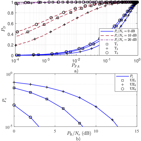
Fig. 6.a shows the receiver operating characteristic (ROC) curves depicting the performance for the three targets across different scenarios. At dB, and , the is for , , and , respectively, while for the non-optimal way the is . This demonstrates that the optimisation improves detection capabilities comparing it with non-optimisation in Fig. 3. Fig. 6.b depicts the BER performance for three UEs versus . The BER decreases as increases for all three UEs, indicating improved communication performance at higher . consistently achieves the lowest BER, followed by and . The performance of the communication subsystem improves significantly with radar waveform optimization. In the non-optimal case, saturates at after 15 dB, as shown in Fig. 2. However, with optimization, drops below by dB across all UEs, due to the communication subsystem’s sensitivity to radar interference, which is better mitigated through optimized waveforms.
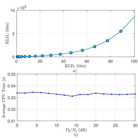
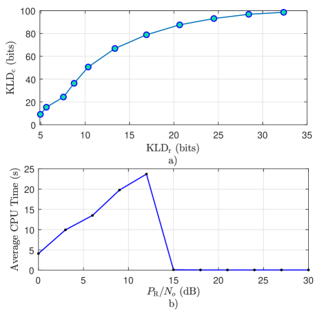
Fig. 7.a illustrates the trade-off performance between radar and communication subsystems using optimized radar waveform. The plot shows versus , with each point on the curve representing a different value. Moving from left to right, both and increase, indicating that higher values lead to improved performance in both subsystems. This visualization provides insights into system behaviour across different levels, highlighting the optimization technique’s robustness in balancing radar and communication performance, we can observe that the optimal way shows an increasing and favourable trade-off, by comparison to the non optimal way in Fig. 4.b, where the saturates at around bits as increases.
Fig. 7.b shows the performance of the radar waveform optimization technique in terms of average CPU time versus . The plot reveals that the computational complexity of the optimization algorithm remains relatively stable across different values. The average CPU time fluctuates slightly between and seconds, with no clear trend of increase or decrease as changes. This suggests that the optimization technique maintains consistent computational efficiency regardless of the values, which is advantageous for practical implementation in varying channel conditions.
VII-C Communication Waveform KLD-based Optimisation
The communication waveform KLD-based optimization algorithm is configured the same as the radar one with a maximum iteration limit of and a convergence tolerance of . The barrier parameter is initialized at , with a barrier reduction factor of . The KLD lower bounds and for all targets and UEs are set to 10 bits.
Fig. 8 illustrates the performance of the radar and communication subsystems when using the optimized communication waveform. Fig. 8.a shows the achievable for each target as a function of for three different power allocation cases: . As increases, improves across all targets in each power allocation scenario, demonstrating enhanced radar performance at higher power-to-noise ratios. For each power allocation, target consistently achieves the highest , followed by and , indicating that the radar performance is influenced by their respective distances or scattering characteristics. Specifically, at dB and , the values are approximately for , , and , respectively. These values increase to about at dB. The linearity observed in improvement beyond 15 dB is consistent across the different values, suggesting stable radar system performance at higher values, despite the suboptimal radar waveform.
Fig. 8.b depicts the communication subsystem performance as represented by versus for three different power allocation cases: . consistently achieves the highest , followed by and , within each power allocation scenario. For dB and , the values are approximately for , , and , respectively. These values increase to around at dB. The communication performance shows less sharp improvement at higher due to the ISAC system’s effort to balance the radar subsystem thresholds with communication subsystem enhancements across different power allocation scenarios.
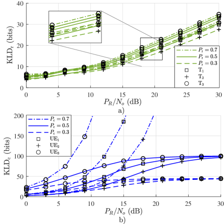
Fig. 9.a shows the ROC curves for the three targets across different scenarios. The ROC curves plot the probability of detection () versus the probability of false alarm () for each target.At dB, and , the is for , , and , respectively, while for the non-optimal way the is . The results demonstrate that communication optimization slightly improves detection capabilities at lower compared to non-optimization, as seen in Fig. 3.
Fig. 9.b depicts the BER performance for three UEs versus . The BER decreases as increases for all three UEs, indicating improved communication performance at higher . consistently achieves the lowest BER, followed by and . The performance of the communication subsystem improves significantly with optimized communication waveform. In the non-optimal case, saturates at after 15 dB, as shown in Fig. 2. However, with optimization, drops below by dB across all UEs, optimized waveforms still provides a gain in comparison to the non-optimal method, however the gain is lower than optimised radar waveform due to the radar interference.
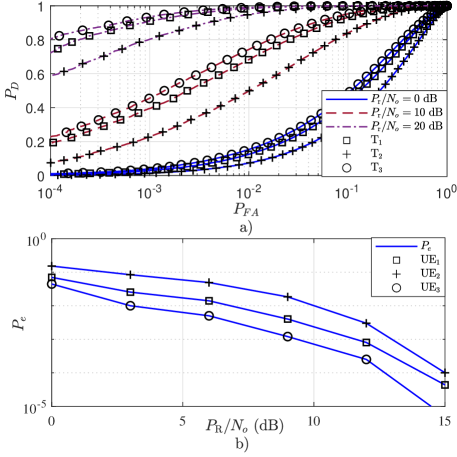
Fig. 10.a illustrates the trade-off between radar and communication subsystems using the optimized communication waveform. The plot shows versus , with each point representing a different value. Moving from left to right, both and increase, indicating that higher values enhance performance in both subsystems. This visualization highlights the robustness of the optimization technique in balancing radar and communication performance across different levels, we can observe that this optimal way shows an increasing and favourable trade-off, by comparison to the non optimal way in Fig. 4.b, where the saturates at around bits as increases.
Fig. 10.b shows the performance of the radar waveform optimization technique in terms of average CPU time versus . The plot reveals that the computational complexity of the optimization algorithm stabilizes after dB values. This is because, at lower , the ISAC system cannot maintain the minimum threshold for all targets and UEs, placing the problem in the infeasible region. Once in the feasible region, the average CPU time fluctuates slightly between and seconds.
VIII Conclusion
In conclusion, this paper has proposed and validated a novel KLD-based framework for optimizing ISAC systems. The two considered optimization techniques, namely, KLD-based radar waveform optimization and KLD-based communication precoding optimization, demonstrated significant improvements over non-optimized scenarios. Radar waveform KLD-based optimization yielded substantial enhancements in both target detection and communication performance, as evidenced by improved ROC curves and reduced BER across all UEs. Communication KLD-based precoding optimization, while primarily benefiting the communication subsystem, also showed modest improvements in radar performance, particularly at lower SNRs. Both techniques exhibited robust performance across varying SNR levels, with radar waveform KLD-based optimization demonstrating stable computational efficiency. Moreover, the trade-off analysis revealed that incorporating the communication signal in radar detection significantly enhances overall ISAC system performance. These findings provide valuable insights for designing and optimizing shared deployment ISAC systems, offering a promising approach to balancing sensing and communication requirements in next-generation wireless networks. The proposed KLD-based framework contributes to the holistic design of ISAC systems, paving the way for more efficient and versatile wireless communications and sensing technologies.
Appendix A Gradient Derivations
This appendix provides detailed derivations for the gradients used in our optimization problem.
A-A Gradients for Radar-Waveform Optimisation
The objective function is given in (39), where the is defined in (36). Therefore, to derive , we first compute . Using the matrix identity , we obtain,
| (58) |
For the trace term, applying yields,
| (59) |
Applying the chain rule to (36), and substituting (58) and (59), we get,
| (60) |
where . Substituting this into (60) and simplifying, we obtain,
| (61) |
Finally, the gradient of with respect to , derived from (39) and (61), is,
| (62) |
For gradient calculations, we consider how changes in affect , where it is defined as follows,
| (63) |
The derivative of with respect to is,
| (64) |
Computing ,
| (65) |
Utilising the chain rule and (64), (65), we obtain,
| (66) |
Therefore, the gradient of with respect to is,
| (67) |
Equations (62) and (67) provide the mathematical foundation for the gradients used in our optimization algorithm.
References
- [1] K. Zheng, Q. Zheng, H. Yang, L. Zhao, L. Hou, and P. Chatzimisios, “Reliable and efficient autonomous driving: the need for heterogeneous vehicular networks,” IEEE Commun. Mag., vol. 53, no. 12, pp. 72–79, 2015.
- [2] D. C. Nguyen et al., “6G Internet of Things: A Comprehensive Survey,” IEEE Internet Things J., vol. 9, no. 1, pp. 359–383, 2022.
- [3] P. Porambage, G. Gür, D. P. M. Osorio, M. Liyanage, A. Gurtov, and M. Ylianttila, “The Roadmap to 6G Security and Privacy,” IEEE Open J. Commun. Soc., vol. 2, pp. 1094–1122, 2021.
- [4] M. Alsabah et al., “6G Wireless Communications Networks: A Comprehensive Survey,” IEEE Access, vol. 9, pp. 148 191–148 243, 2021.
- [5] ERICSSON, “Joint communication and sensing in 6G networks,” Technical Report, Oct. 2021. [Online]. Available: https://tinyurl.com/wt5t7dwd
- [6] N. Rajatheva et al., “White Paper on Broadband Connectivity in 6G,” arXiv preprint arXiv:2004.14247, 2020. [Online]. Available: https://doi.org/10.48550/arXiv.2004.14247
- [7] M. M. Azari et al., “Evolution of Non-Terrestrial Networks From 5G to 6G: A Survey,” IEEE Commun. Surv. Tutor., vol. 24, no. 4, pp. 2633–2672, 2022.
- [8] A. Liu et al., “A Survey on Fundamental Limits of Integrated Sensing and Communication,” IEEE Commun. Surveys Tuts., vol. 24, no. 2, pp. 994–1034, 2022.
- [9] F. Liu, C. Masouros, A. Li, and T. Ratnarajah, “Robust MIMO Beamforming for Cellular and Radar Coexistence,” IEEE Wireless Commun. Lett., vol. 6, no. 3, pp. 374–377, 2017.
- [10] F. Liu, L. Zhou, C. Masouros, A. Li, W. Luo, and A. Petropulu, “Toward Dual-functional Radar-Communication Systems: Optimal Waveform Design,” IEEE Trans. Signal Process., vol. 66, no. 16, pp. 4264–4279, 2018.
- [11] M. Temiz, E. Alsusa, and M. W. Baidas, “A Dual-Functional Massive MIMO OFDM Communication and Radar Transmitter Architecture,” IEEE Trans. Veh. Technol., vol. 69, no. 12, pp. 14 974–14 988, 2020.
- [12] ——, “Optimized Precoders for Massive MIMO OFDM Dual Radar-Communication Systems,” IEEE Trans. Commun., vol. 69, no. 7, pp. 4781–4794, 2021.
- [13] J. A. Zhang et al., “An Overview of Signal Processing Techniques for Joint Communication and Radar Sensing,” IEEE J. Sel. Topics Signal Process., vol. 15, no. 6, pp. 1295–1315, 2021.
- [14] F. Liu, C. Masouros, A. Li, H. Sun, and L. Hanzo, “MU-MIMO Communications With MIMO Radar: From Co-Existence to Joint Transmission,” IEEE Trans. Wireless Commun., vol. 17, no. 4, pp. 2755–2770, 2018.
- [15] C. Xu, B. Clerckx, and J. Zhang, “Multi-Antenna Joint Radar and Communications: Precoder Optimization and Weighted Sum-Rate vs Probing Power Tradeoff,” IEEE Access, vol. 8, pp. 173 974–173 982, 2020.
- [16] N. Fatema, G. Hua, Y. Xiang, D. Peng, and I. Natgunanathan, “Massive MIMO Linear Precoding: A Survey,” IEEE Syst. J., vol. 12, pp. 3920–3931, 2018.
- [17] C. Ouyang, Y. Liu, and H. Yang, “Performance of Downlink and Uplink Integrated Sensing and Communications (ISAC) Systems,” IEEE Wireless Communications Letters, vol. 11, no. 9, pp. 1850–1854, 2022.
- [18] B. Tang, M. M. Naghsh, and J. Tang, “Relative Entropy-Based Waveform Design for MIMO Radar Detection in the Presence of Clutter and Interference,” IEEE Trans. Signal Process., vol. 63, no. 14, pp. 3783–3796, 2015.
- [19] J. Tang, N. Li, Y. Wu, and Y. Peng, “On Detection Performance of MIMO Radar: A Relative Entropy-Based Study,” IEEE Signal Process. Lett., vol. 16, no. 3, pp. 184–187, 2009.
- [20] Y. Kloob, M. Al-Jarrah, E. Alsusa, and C. Masouros, “Trade-Off Performance Analysis of Radcom Using the Relative Entropy,” in Proc. IEEE Symp. Comput. Commun. (ISCC) 2024, pp. 1–6, 2024.
- [21] M. Al-Jarrah, E. Alsusa, and C. Masouros, “A Unified Performance Framework for Integrated Sensing-Communications based on KL-Divergence,” IEEE Trans. Wireless Commun., pp. 1–1, 2023.
- [22] ——, “Kullback-Leibler Divergence Analysis for Integrated Radar and Communications (RadCom),” in 2023 IEEE Wireless Commun. Netw. Conf. (WCNC), 2023, pp. 1–6.
- [23] Y. Kloob, M. Al-Jarrah, E. Alsusa, and C. Masouros, “Novel KLD-based Resource Allocation for Integrated Sensing and Communication,” IEEE Trans. Signal Process., vol. 72, pp. 2292–2307, 2024.
- [24] Z. Fei, S. Tang, X. Wang, F. Xia, F. Liu, and J. A. Zhang, “Revealing the trade-Off in ISAC systems: The KL divergence perspective,” IEEE Wireless Commun. Lett., pp. 1–1, 2024.
- [25] F. Liu, Y.-F. Liu, A. Li, C. Masouros, and Y. C. Eldar, “Cramér-Rao Bound Optimization for Joint Radar-Communication Beamforming,” IEEE Trans. Signal Process., vol. 70, pp. 240–253, 2022.
- [26] X. Wang, Z. Fei, J. A. Zhang, and J. Xu, “Partially-Connected Hybrid Beamforming Design for Integrated Sensing and Communication Systems,” IEEE Trans. Commun., vol. 70, no. 10, pp. 6648–6660, 2022.
- [27] Z. Liao and F. Liu, “Symbol-Level Precoding for Integrated Sensing and Communications: A Faster-Than-Nyquist Approach,” IEEE Communications Letters, vol. 27, no. 12, pp. 3210–3214, 2023.
- [28] A. Hassanien, M. G. Amin, Y. D. Zhang, and F. Ahmad, “Signaling strategies for dual-function radar communications: an overview,” IEEE Aerosp. Electron. Syst. Mag., vol. 31, no. 10, pp. 36–45, 2016.
- [29] P. Kumari, J. Choi, N. González-Prelcic, and R. W. Heath, “IEEE 802.11ad-Based Radar: An Approach to Joint Vehicular Communication-Radar System,” IEEE Trans. Veh. Technol., vol. 67, no. 4, pp. 3012–3027, 2018.
- [30] H. Xu, R. S. Blum, J. Wang, and J. Yuan, “Colocated MIMO radar waveform design for transmit beampattern formation,” IEEE Trans. Aerosp. Electron. Syst., vol. 51, no. 2, pp. 1558–1568, 2015.
- [31] A. Hassanien and S. A. Vorobyov, “Phased-MIMO Radar: A Tradeoff Between Phased-Array and MIMO Radars,” IEEE Trans. Signal Process., vol. 58, no. 6, pp. 3137–3151, 2010.
- [32] H. Zhang, B. Zong, and J. Xie, “Power and Bandwidth Allocation for Multi-Target Tracking in Collocated MIMO Radar,” IEEE Trans. Veh. Technol., vol. 69, no. 9, pp. 9795–9806, 2020.
- [33] H. Zhang, J. Shi, Q. Zhang, B. Zong, and J. Xie, “Antenna Selection for Target Tracking in Collocated MIMO Radar,” IEEE Trans. Aerosp. Electron. Syst., vol. 57, no. 1, pp. 423–436, 2021.
- [34] W. Yi, T. Zhou, Y. Ai, and R. S. Blum, “Suboptimal Low Complexity Joint Multi-Target Detection and Localization for Non-Coherent MIMO Radar With Widely Separated Antennas,” IEEE Trans. Signal Process., vol. 68, pp. 901–916, 2020.
- [35] E. Fishler, A. Haimovich, R. Blum, L. Cimini, D. Chizhik, and R. Valenzuela, “Spatial Diversity in Radars—Models and Detection Performance,” IEEE Trans. Signal Process., vol. 54, no. 3, pp. 823–838, 2006.
- [36] J. Nocedal and S. J. Wright, Numerical Optimization, 2nd ed. Springer, 2006.
- [37] D. P. Bertsekas, Nonlinear Programming, 2nd ed. Athena Scientific, 1999.
- [38] L. Armijo, “Minimization of functions having Lipschitz continuous first partial derivatives,” Pacific Journal of Mathematics, vol. 16, no. 1, pp. 1–3, 1966.
- [39] A. Forsgren, P. E. Gill, and M. H. Wright, “Interior Methods for Nonlinear Optimization,” SIAM Review, vol. 44, no. 4, pp. 525–597, 2002. [Online]. Available: https://doi.org/10.1137/S0036144502414942