A general machine learning model of aluminosilicate melt viscosity and its application to the surface properties of dry lava planets

Abstract

Ultra-short-period exoplanets like K2-141 b likely have magma oceans on their dayside, which play a critical role in redistributing heat within the planet. This could lead to a warm nightside surface, measurable by the James Webb Space Telescope, offering insights into the planet’s structure. Accurate models of properties like viscosity, which can vary by orders of magnitude, are essential for such studies.

We present a new model for predicting molten magma viscosity, applicable in diverse scenarios, including magma oceans on lava planets. Using a database of 28,898 viscosity measurements on phospho-alumino-silicate melts, spanning superliquidus to undercooled temperatures and pressures up to 30 GPa, we trained a greybox artificial neural network, refined by a Gaussian process. This model achieves high predictive accuracy (RMSE $\approx 0.4\log_{10}$ Pa$\cdot$s) and can handle compositions from SiO₂ to multicomponent magmatic and industrial glasses, accounting for pressure effects up to 30 GPa for compositions such as peridotite.

Applying this model, we calculated the viscosity of K2-141 b’s magma ocean under different compositions. Phase diagram calculations suggest that the dayside is fully molten, with extreme temperatures primarily controlling viscosity. A tenuous atmosphere (0.1 bar) might exist around a 40° radius from the substellar point. At higher longitudes, atmospheric pressure drops, and by 90°, magma viscosity rapidly increases as solidification occurs. The nightside surface is likely solid, but previously estimated surface temperatures above 400 K imply a partly molten mantle, feeding geothermal flux through vertical convection.

Keywords magma  $\cdot$ viscosity  $\cdot$ pressure  $\cdot$ machine learning  $\cdot$ magma ocean  $\cdot$ exoplanet  $\cdot$ K2-141 b

1 Introduction

Magma oceans are recognised as key phenomena shaping the internal structure and secondary atmospheres of rocky planets [1, 2, 3, 4, 5]. While primarily theoretical, spectroscopic observations of ultra-short period (USP) exoplanets [e.g. 55 Cnc e and K2-141b; see for a review 6] may help shed light on their nature and longevity. Indeed, these planets, known as "lava planets", are thought to host vast oceans of molten silicate rocks, a.k.a. magma oceans, on their dayside because of intense stellar irradiation producing dayside temperatures well above 2000 K [7, 8, 9, 10, 11]. Outgassing from these magma oceans is expected to significantly influence the planet’s atmospheric composition, introducing elements such as H, C, N, Si, Fe, Na, and K [e.g. 12]. Therefore, observing the atmospheres of lava planets using spectroscopic methods may provide indirect data documenting the presence and composition of magma oceans. To do so requires a sound understanding of the interactions between the molten mantle and the atmosphere of a lava planet. Combining fluid dynamics simulations [e.g., 13, 14, 15] with outgassing and atmosphere models [16, 12, 17] are promising avenues by which this can be achieved. Despite the abundance of new spectroscopic data  [e.g., see 18, 19, 20, 21, 16, 22, for 55 Cnc e] via MIRI and nirSpec on the James Webb Space Telescope, interpreting these data in a geodynamic and geochemical context remain challenging.

This is because information as to the key physical parameters that dictate the behaviour of magma oceans is currently missing. Chief among these is magma viscosity ($\eta$, Pa·s). It controls melt mobility and elemental diffusion timescales, and thus the vigor of thermal convection and magma outgassing. Through experimental studies, it has been shown that magma viscosity varies non-linearly over more than 15 orders of magnitude with temperature, melt chemical composition (including volatile concentration), crystal and bubble fractions, and pressure [23, 24, 25, 26, 27, 28, 29, 30, 31], posing a significant challenge for accurate calculations.

Various models have been developed to calculate the viscosity of crystal and bubble free silicate melt [32], including empirical parametric models [33, 34, 35, 36, 28, 37, 38], high accuracy models for specific compositions [e.g. 39, 40, 41, 42], and models based on specific theoretical frameworks [43, 44, 45, 46]. Recently, machine learning (ML) has shown promise in predicting viscosity for geological and glass-forming melts [47, 48, 49, 50, 51, 52]. Regardless of the method, most existing models focus on predicting the viscosity of crystal-free melts at room pressure over a restrained compositional domain (e.g. industrial or geologic compositions), neglecting the effects of high pressures, crystals, and bubbles – conditions likely encountered on USP planets.

No existing model can predict magma viscosity across the wide range of melt compositions ($X$), temperatures ($T$), and pressures ($P$) found on USP planets, where compositions could range from Earth-like to refractory or even carbon-rich  [7, 18, 11], and where temperatures vary greatly between day and night sides  [e.g. 7, 8, 53]. Besides, $P$ may exceed those found in the Earth given that the masses of super-Earths are up to 10 times as massive as Earth [8]. Predicting the properties of molten rocks under such conditions require a new generation of models that leverage as much as possible the existing data on alumino-silicate (sensus latto) compositions.

In this study, we present a new database of experimental viscosity measurements as a function of $T$ and $P$ for melts with diverse compositions in the system SiO₂-FeO-Fe₂O₃-TiO₂-Al₂O₃-MnO-MgO-CaO-Na₂O-K₂O-P₂O₅-H₂O. We benchmark ML models to predict magma viscosity and propose a new model combining a Gaussian process with a greybox artificial neural network to calculate melt viscosity and associated uncertainties. We then apply this model for the calculation of the rheology of the magma ocean at the surface of K2-141 b [54, 55], a dry (i.e. no thick atmosphere) USP planet. We further assess the impact of internal temperature on the nightside surface, potentially allowing inferences about the interior state of dry lava planets from nightside temperature measurements.

2 Materials and Methods

In this study, we aim at performing the following task. Given $T$, $P$ and $X$, a machine learning model $G$ containing a set of adjustable parameters $m$ will calculate $\log_{10}\eta$ as

$$\log_{10}\eta=G(T,P,X,m)$$ (1)

The adjustable parameters $m$ will be learned during a training phase. It consists in solving a least-square regression problem: given experimental $\eta$ measurements at known $T$, $P$ and $X$ conditions, we adjust the parameters $m$ via gradient descent to minimize the root-mean square error (RMSE) between model predictions and measurements. Therefore, to implement a machine learning model of silicate melt viscosity, we need a dataset that will be prepared prior to training a machine learning model. Many different ML models can be used to solve the present problem. We will benchmark the performance of a few selected models to determine which one may be most appropriate for the task at hand. Those steps are described in the following sub-sections.

2.1 Dataset

As a starting point, we used the database of i-Melt [50, 52], which includes viscosity versus temperature measurements for 790 melt compositions in the system Na₂O-K₂O-CaO-MgO-Al₂O₃-SiO₂. This database was enhanced by a survey of the existing literature, targeting multi-component compositions including the additional elements FeO, Fe₂O₃, TiO₂, MnO, P₂O₅ and H₂O. As of 25/09/2024, this database comprises 15,440 viscosity measurements in the range 10^-3 - 10¹⁵ Pa·s for 2,155 melt compositions different by at least 0.1 mol% at room pressure, and 1,227 viscosity measurements for 243 melt compositions at high pressures, up to 30 GPa. It represents the compilations of data from 245 publications. When available, the fractions of iron as ferrous and ferric were compiled. When not available, those were calculated using the Borisov model [56]; in the case no oxygen fugacity details were provided in the publications, we assumed that melt viscosities were measured in air. The following features thus are available in the database: the molar proportions of SiO₂, TiO₂, Al₂O₃, FeO, Fe₂O₃, MnO, MgO, CaO, Na₂O, K₂O, P₂O₅, H₂O, pressure in GPa, temperature in Kelvin, and viscosity in log₁₀ Pa·s. The database together with the list of references is available on the IPGP Data Repository [57]. We further enhanced this database by getting data from the SciGlass database using the GlassPy library [58]. From SciGlass, we only extracted data for melt compositions that do not appear in the original database. This represents the addition of 12,231 data points from 3,591 compositions (different by at least 0.1 mol%). Figure 1 provides a visual summary of the database, in which the number of compositions including the various elements are visible, together with the viscosity versus temperature and pressure coverage.

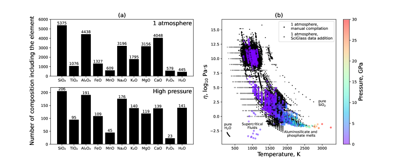
Figure 1: (a) Bar plots showing the number of compositions including a particular oxide component in the database. (b) Viscosity versus temperature diagram showing all data from the full database. Data from the SciGlass database are shown in grey. Colored symbols indicate high pressure data.

2.2 Data Preparation

Prior to any calculation, we separated the dataset in three training (80%), validation (10%) and testing (10%) subsets. The training subset is used for training the algorithms and the validation subset for tuning the model hyperparameters via Bayesian optimisation (see below). The testing subset contains data that are not used during training and hyperparameter tuning, such that it will allow evaluating the predictive uncertainties of the different methods.

For performing the splits, we first separated the dataset in two room pressure and high pressure datasets, because the compositional coverage and the number of data at room and high pressures are very different and skewed towards the former. For room pressure data, we adopted a stratified group splitting approach that ensures that each subset will contain different compositions in relatively balanced proportions [see 52, for details]. For high pressure data, we did not use this method because the high pressure dataset contains too few compositions, with only a few data points at different pressures per composition. Considering that the compositional domain will be already well covered and represented in the different room pressure data subsets, and that the aim of the high pressure data is to provide knowledge about the effect of pressure, we decided to split randomly the high pressure data in the training, validation and testing data subsets regardless of melt compositions. To perform the different random splits, we selected optimal random seeds such that the training, validation and test subsets present similar statistical distributions of their features. To do so, we tried 1,500 different random seeds, and selected the 10 ones that ensured the lowest Wasserstein distances of the feature distributions between the various data subsets. Then, among those seeds, we rejected those that resulted in including end-member compositions (e.g., SiO₂ or H₂O) in the validation or testing data subsets. We then selected an appropriate seed given this constrain and the Wasserstein distances test. This approach ensures the similarity of the data distributions between the different training, validation and test data subsets. Finally, after data splitting, the high and low pressure parts of the training-validation-testing data subsets were concatenated.

T, P and melt composition X can be provided as inputs to a machine learning model (eq. 1). Such variables are called features in the ML jargon. To improve the performance of ML models, new features may be added. For the present problem, those could be for instance the glass non-bridging oxygen to tetrahedral ratio NBO/T or its optical basicity. We tested the addition of various new features but this did not improve the accuracy of model predictions of melt viscosity at known conditions. We thus did not add new features for this work. All models were trained using the following features: T in K, P in GPa, and the fractions of oxide components SiO₂, TiO₂, Al₂O₃, FeO, Fe₂O₃, MnO, MgO, CaO, Na₂O, K₂O, P₂O₅, and H₂O.

A final data preparation step entailed scaling the datasets. For the blackbox algorithms, each feature was scaled by removing its mean and dividing it by its variance (a.k.a. standard scaling). For the Gaussian process and greybox artificial neural network models (see below), we used a custom explicit scaling: features were 1000./T (K), P/30. (GPa), and oxide fractions.

2.3 Machine learning models

Many different ML models can be appropriate for performing the task described by equation 1. In this work, we benchmark six different models. First, we selected four different archetypal supervised regression models easy to implement using the SciKit Learn library [59]:

• the LR model is a simple linear regression model that will be used as a baseline model,

• the SVR model uses support vector machine regression,

• the RF model uses a random forest algorithm,

• and the ANN model is a feed-forward artificial neural network model.

These classical models are described in machine learning textbooks [60, 61], to which we refer the readers for exhaustive descriptions. Briefly, the LR model will establish a linear relationship between inputs ($T$, $P$ and $X$) and outputs ($\log_{10}\eta$). The SVR model will attempt performing the same task, but after projecting the data in a hyperspace using a mathematical trick called the kernel trick. Non-linear relationships become linear on such a hyperplane, such that SVR models have the ability to reproduce non-linear relationships between inputs and outputs. The RF model is an ensemble learning method that operates by constructing a multitude of decision trees at training time and outputting the average prediction of the individual trees at inference time. It is particularly suited to help in addressing the non-linearity and complex interactions between variables. Finally, the ANN model consists of interconnected nodes (a.k.a. neurons) that ‘react’ differently to their inputs, thanks to non-linear activation functions (e.g., tanh or sigmoid) used to modulate the response of each node to its inputs. This is a foundation structure used in many complex deep learning models, including those for the prediction of the viscosity of glass-forming melts [49, 51, 62, 50, 52, 48].

Then, we test a greybox artificial neural network (hereafter called Greybox ANN) model that embeds the Vogel-Tamman-Fulcher [23] equation:

$$\log\eta=A+\frac{B}{T-C}\,,$$ (2)

with $T$ the temperature in K, $A$ a common adjustable parameter [35, 63, 28], and $B$ and $C$ adjustable parameters that depend on melt composition $X$ and pressure $P$. The artificial neural network predicts $A$, $B$ and $C$ given $P$ and $X$, then equation 2 is used to calculate $\log_{10}\eta$ as a function of $T$. The $\log_{10}\eta$ versus $T$ dependence is thus constrained in the model through the use of equation 2. This injects domain knowledge in the model and ensures reliable extrapolations at high temperatures, for instance in conditions pertinent for exoplanetary magma oceans. Other equations can be used, as in the more complex model i-Melt [50, 52, 64], a multitask greybox machine learning model that predicts various properties of alkali and alkaline-earth aluminosilicate melts. Here we chose the VFT equation as it is a simple and well established one that has proven its usefulness in viscosity modeling [28].

Finally, we test the use of a Gaussian process (GP) regression model. A GP is a collection of random variables, any finite number of which have consistent joint Gaussian distributions [65]. Another way of describing a GP is that it places a probability density over functions. Here, we are interested in calculating the probability density of the function that describes how melt viscosity varies with $T$, $P$ and $X$. We do not know this function, but the observations can allow its probability density to be constrained. A GP is fully defined by its mean $m(x)$ and covariance $k(x,x^{\prime})$ functions:

$$f(x)\sim GP(m(x),k(x,x^{\prime}))\,.$$ (3)

$k(x,x^{\prime})$ is also known as the kernel function. It allows placing a distribution over functions. Its choice is critical as it embeds the mathematical formalism to describe how smooth and how variable is the expected function. For instance, a linear kernel implies that the target function is linear. For placing a probability distribution over non-linear functions, one will choose a non-linear kernel such as the squared exponential. Kernels can be multiplied and added, to create complex kernel functions that can reproduce very different shapes of functions. $k(x,x^{\prime})$ usually has hyper-parameters that will control the behavior of the function (smoothness, periodicity, etc.) and that can be adjusted by gradient-based optimisation. For more details regarding kernel design and selection, see [65].

The mean function usually is chosen as a constant value equal to 0 in most applications. This is because the mean function is directly updated as we perform predictions on new points $x^{*}$. It thus usually does not have a strong influence on posterior predictions at those new values $x^{*}$. However, in the present case, we are dealing with a rather sparse data coverage of a large multidimentional problem. We further may want to extrapolate predictions at the high temperatures typical of exoplanetary magma oceans (2300-3000 K). In such a case, setting $m(x)=0$ is not the best choice because upon extrapolating, the GP will tend toward the initial value of m(x). If it is set to 0, it thus will tend toward 0. To avoid this, prior information about the problem can be provided in the mean function [65, 66, 67], in the form of known analytical equations or of a model. In the present case, an appropriate mean function $m(x)$ could be the VFT equation 2, but it only accounts for the temperature effect on melt viscosity and thus it is difficult to use it as is. To solve this problem, the mean function we use is the greybox feed-forward artificial neural network previously described. The Greybox ANN predictions are used as prior estimates of $\log_{10}\eta$ given $T$, $P$ and $X$. Then, during inference, the GP will update this prior estimate using the kernel function $k(x,x^{\prime})$ and the data to provide posterior values of viscosity at the new desired $P$-$T$-$X$ conditions.

The interest of GPs in this work is twofold: first, using appropriate kernels and mean functions, we ensure model smoothness and can leverage domain knowledge, and, second, the GP formalism allows calculating uncertainties on posterior predictions. Uncertainties can be obtain from artificial neural network, using various methods such as Monte Carlo Dropout and Conformal predictions [for details and an application see 52, 64], but those are not necessarily straightforward to implement. GP predictions are rooted in Bayesian statistics and the mathematical formalism is well established. GP thus provides reliable prediction uncertainties, an important point for evaluating the quality of predictions.

2.4 Hyperparameter tuning and model training

To tune the hyperparameters of the models, we monitored the root-mean-squared errors (RMSEs) on the training and validation data subsets. The hyperparameters of the LR, SVR and RF models were tuned using the Scikit-Optimize library, which allows easy tuning of hyperparameters through the use of Bayesian optimization. For the ANN model, after some manual tests and a grid search, we selected a simple yet effective architecture composed of two layers of 200 ReLU activation units [68].

The Greybox ANN was implemented using the PyTorch machine learning library [69]. Its architecture was selected to be the same as the ANN model, because tests showed that it performed well. However, as in i-Melt [52], the model relies on GELU activation functions [70]. During training, early stopping and dropout [71] were adopted to prevent overfitting.

The GP model is implemented using the GPyTorch library [72]. Different kernels were tested. Those tests indicate that a Matérn 5/2 kernel with 14 different lengthscales performed well. As explained previously, the mean function of the GP is provided by pre-trained Greybox ANN models.

The final training of the different models with optimal hyperparameters was performed combining the training and validation data subsets, except for the Greybox ANN because early stopping uses the validation dataset during training. For the Greybox ANN and the GP, training may not always proceed well due to the stochasticity in artificial neural network training. This problem is solved by performing 100 different training runs. From those runs, we then selected the models for which the metrics were the lowest for the Greybox ANN. The code to replicate this study is available on Github (https://charlesll.github.com/gpvisc). The library gpvisc [73] allows using the Greybox ANN and GP models to perform predictions in new situations via Python coding or a more convenient GUI interface.

3 Results

3.1 Performance evaluation

Over the very broad range of compositions we investigate (Fig. 1), the different models predict the viscosity of melts with variable levels of performance. Table 1 reports the root-mean-squared-errors (RMSE), mean absolute error (MAE), and coefficient of regression ($R^{2}$) for the different methods and data subsets. Errors on the test data subset are indicative of predictive errors because the models did not see melt compositions included in this data subset. We further report the metrics for the test data subset excluding data points from SciGlass (Test^∗ column) because those are know to be of variable quality [e.g. 74]. Our hand-curated database is of better quality, and error metrics on it may be more indicative of true model errors.

Model	Metric	Training-Validation	Test	Test∗
Linear regression (LR)	RMSE	1.58	1.58	1.51
	MAE	1.08	1.09	0.91
	R2	0.873	0.872	0.903
Support Vector Machine (SVM)	RMSE	0.46	0.53	0.36
	MAE	0.09	0.15	0.13
	R2	0.989	0.986	0.994
Random Forest (RF)	RMSE	0.19	0.54	0.37
	MAE	0.05	0.14	0.13
	R2	0.998	0.985	0.994
Artificial Neural Network (ANN)	RMSE	0.33	0.43	0.33
	MAE	0.14	0.17	0.15
	R2	0.994	0.990	0.995
Greybox Artificial Neural Network (Greybox ANN)	RMSE	0.42 - 0.55	0.48	0.33
	MAE	0.18 - 0.21	0.19	0.18
	R2	0.991 - 0.984	0.988	0.995
Gaussian process (GP)	RMSE	0.35	0.44	0.32
	MAE	0.12	0.15	0.14
	R2	0.994	0.990	0.996

Table 1: Root Mean Squared Error (RMSE), Median Absolute Error (MAE) and coefficient of determination $R^{2}$ of the different models. For final training of the algorithms after hyperparameter optimization, the training and validation data subsets were joined. The RMSE on the joined training-validation dataset is shown here, except for the Greybox ANN model. For this model, we always monitor the metrics on the validation dataset to perform early stopping and avoid overfitting, such that we report the RMSE on the three data subsets. The second Test^∗ column indicates the metrics for the hand-curated part of the test data subset, excluding SciGlass values.

Metrics indicate that the linear regression LR model performs poorly, with RMSE higher than 1 order of magnitude (Table 1). This is expected because the melt viscosity dependence on temperature, pressure and melt chemical composition is highly non-linear. As a result, non linear ML models such as SVM and RF perform much better, with test RMSE of 0.53 and 0.54, respectively. The RF model has an issue though: the RMSE on the dataset used for training is significantly lower than the test RMSE. This indicates that this model overfits its training data, and thus its predictions may not be very reliable.

The feed-forward artificial neural network ANN performs very well with minimal overfitting as indicated by close training-validation and testing RMSEs, respectively of 0.33 and 0.43 (test error of 0.33 excluding SciGlass data). This indicates that artificial neural networks are the method of choice for the problem at hand; a result that is not unexpected when considering their success in previous studies [48, 49, 75, 47, 52, 51].

The Greybox ANN model performs well with minimal overfitting, as indicated by good metrics (Table 1). Those are slightly higher than those of the blackbox ANN. This is probably due to a slight decrease in model flexibility resulting from the enforcement of the $T$ versus $\log_{10}\eta$ relationship through equation 2 in the Greybox ANN model. However, this apparent disadvantage actually is a strength: the Greybox ANN model will always provide physically-realistic viscosity predictions as a function of temperature, even in the high temperature range of magma oceans.

The GP model, based on the combination of the Greybox ANN with a Gaussian process, shows very good predictive performance (Table 1), with a RMSE on the test dataset of 0.44 $\log_{10}Pa\cdot s$ (0.32 $\log_{10}Pa\cdot s$ when excluding SciGlass data). The model overfits very slightly its training dataset (RMSE = 0.34) but this remains acceptable. The metrics indicate that, overall, this model outperforms the others.

3.2 Model selection

A closer inspection of the predictions performed by the models reveals that some models are more appropriate for the problem at hand. In particular, predicted viscosities should be continuous functions of intensive variables; that is, pressure and temperature. To evaluate this point, melt viscosity is first represented as a function of $T$ for a given melt composition (Fig. 2). In this representation, data tend to cover specific regions (Fig. 1) as most melts crystallize at $\eta$ comprised between $\approx 10^{5}$ and $\approx 10^{8}$ Pa$\cdot$s. This test confirms that the LR model is not appropriate (Fig. 2a), as expected from its performance metrics (Table 1). The SVM model provides smooth predictions of viscosity, but with small deviations at $\eta>10^{5}$. The RF model only provides sensible results in regions where data are present. Its predictions are not smooth, sometimes leading to unexpected behavior as visible here at high $\eta$ values (Fig. 2a). The RF model thus is not appropriate for the present problem, at least in its current simple implementation (more complex implementations are out of the scope of this work).

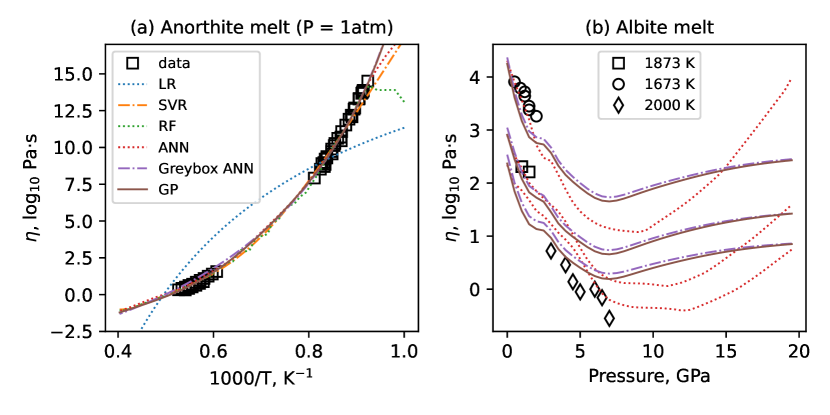
Figure 2: Viscosity against reciprocal temperature of an anorthite melt (a), and against pressure for albite melt (b). Symbols are measurements from [76, 77, 78, 79, 80, 81, 82], and lines are model predictions (see legend). Only the predictions of the three best models are represented in (b).

The ANN, Greybox ANN and GP models all present smooth, realistic predictions of $\eta$ as a function of $T$, even outside of the data calibration range (Fig. 2a), and, indeed as a function of $P$ and composition. The RMSE between calculations and measurements at high pressure is of 0.58 for the GP model and of 0.62 for the Greybox ANN (all high pressure data considered). In figure 2b, we show examples of the performance of these models for the prediction of the viscosity of albite melt with pressure at 1673, 1873 and 2000 K. In the range where data are present, the three models yield consistent, smooth predictions. The GP model predictions are a slight refinement of the Greybox ANN model predictions. Above 7 GPa where data are not present for albite melt, the ANN and GP/Greybox ANN models predict diverging values. This reflects the lack of data: the models are extrapolating outside their training range and predictions should be taken with caution (see Discussion).

Among tested models, the Greybox ANN and the GP are favored due to their predictive power (Table 1). Besides, both embed domain knowledge through the use of equation 2, this improving the robustness of their predictions. In general, the GP model should be favored as its metrics are slightly better and as it provides uncertainties on predictions. However, in some rare cases, we observed that the Greybox ANN model offered more physically-sound predictions, for instance when asking to predict $\eta$ at high temperature for water-bearing melts (see example notebooks at [73]). Another case of preference for using the Greybox ANN model is when there is a critical need for speed. Indeed, predictions using this model are faster and more memory efficient than those performed using the GP model. Performing inference using the GP on 10 data points requires approximately 294 milliseconds on a 13th Gen Intel® Core™ i9-13900K CPU and 12 milliseconds on a NVIDIA RTX A4500 GPU. Using the Greybox ANN, the same query is performed in approximately 524 microseconds on the CPU and 282 microseconds on the GPU. The GP predictions are fast, but it is clear that the Greybox ANN model is faster. Therefore, in very intensive fluid dynamic calculations that do not require predictions with uncertainties, it could be desirable to use the Greybox ANN model. The gpvisc library [73] allows easily getting predictions from both models, as the Greybox ANN is simply the mean function of the GP model. For the following analysis in this paper, we will use the GP model as we will be able to take into account of model uncertainties in our analysis.

3.3 High pressure predictions

We explore in more detail the high pressure predictions using the GP model in Figure 3. We first observe systematically robust predictions of high and low melt viscosities (Fig. 3a). The model reproduces well (within half a log unit) the viscosity variations with pressure (up to 7 GPa) of a polymerised albite melt (Fig. 3b) as well as of ultramafic compositions of significance for magma oceans such as CaSiO₃ and peridotite (Fig. 3b,c). Indeed, for peridotitic melts, we observe that the model closely reproduces existing data up to 30 GPa.

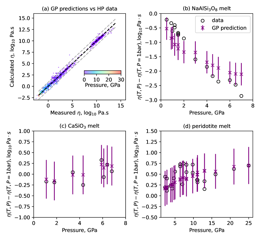
Figure 3: (a) Calculated viscosity with the GP model versus measurements. The black dashed line represent the 1:1 correspondence, and the grey dashed lines the average 95 % confidence interval ($\pm 0.9$). (b), (c) and (d) Comparison between Gaussian process (GP) viscosity predictions and data on albite NaAlSi₃O₈, wollastonite CaSiO₃ and peridotite melts. The viscosity at high pressure and high temperature ($\eta(T,P)$) is represented relative to that at the same temperature and 1 bar ($\eta(T,P=1\,bar)$, calculated from an interpolative fit of experimental data with the Vogel-Tammann-Fulcher equation). Experimental viscosity measurements data from [80, 81, 82, 83, 84, 85].

Despite the promise shown in the model results, we should bear in mind that the high pressure dataset is small and sparse in terms of pressure and compositional coverage. The good predictive performance of the model for a composition such as peridotite does not imply that the model can predict viscosity across a range of melt compositions up to 30 GPa.

3.4 Limitations

The main limitation of ML models is that they are interpolative by nature. Therefore, when asked to predict values for inputs far outside the range of the training data, the returned values may be erroneous. At 1 bar, the compositional dataset is broad and the temperature dependence of melt viscosity is constrained by the use of eq. 2 in the Greybox ANN and GP models. It thus is unlikely that users ask the GP model to extrapolate at 1 bar. However, it still is possible. To illustrate what happens in such a case, we report in Fig. 4a the viscosity of a sodium silicate melt as a function of its concentration in silica. Predictions from three different GP models are reported. Indeed, different training runs yield slightly different models, and we can leverage this stochasticity to test the robustness of model predictions. The three GP models have comparable test RMSE values that are equal to or lower than 0.45. We observe that above 50 mol% silica, where data are available, the three models yield very similar predictions and agree within uncertainty. Below 50 mol%, we see that predictions largely diverge. This indicates that models are providing predictions for compositions outside their training range. We note that this behavior also indicates that Greybox ANN models do not provide sensible predictions for compositions outside the training range. Indeed, the behavior of the GP model in the extrapolative regim is directly due to that of the Greybox ANN used as its mean function, because a Gaussian process falls back to its mean function value if no data are present to constrain its predictions.

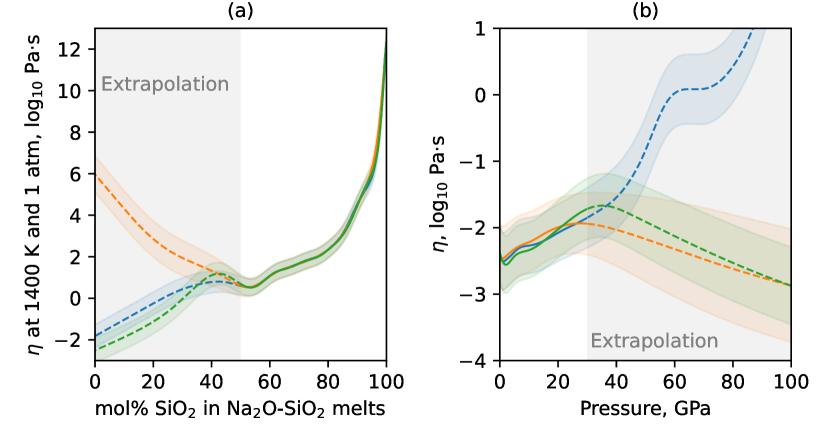
Figure 4: (a) Viscosity in Na₂O-SiO₂ melts as a function of the silica content. (b) Viscosity at 3000 K as a function of temperature for peridotite melt. Lines are predictions from three GP models; solid lines indicate that the models worked in interpolative regime, dashed lines indicate extrapolations. The grey shaded region indicates the region in which no data was available.

We perform the same test at high pressure for a peridotite melt viscosity at T = 3000 K (Fig. 4b). Below 30 GPa, predictions from the three GP models are comparable. Above 30 GPa, the three GP models yield very distinct, and possibly wrong predictions. As for the previous test, this indicates that the GP models are providing predictions for pressures outside the training range for this composition.

From those tests, we see that the behavior of the Greybox ANN and GP models should be checked in case of extrapolation. We stress that, given the sparsity of the high pressure dataset, such extrapolative behavior could be reached very easily for melt compositions that deviate from those present in the training dataset. This could be improved by the addition of a term in equation 2 to account for the effect of $P$. For instance, [86, 42] proposed the addition of linear pressure dependence terms in equation 2. However, this will not work in all cases as we expect a turnover of the dependence of melt viscosity on pressure as a function of melt polymerisation [87]. This area requires further work to be improved.

In case of doubt, the robustness of the predictions can be tested by querying predictions from a few different GP models (Fig. 4). The gpvisc library [73] provides three trained Greybox ANN and associated GP models to do so, with examples. The test should be performed in case of doubt, because unfortunately the error bars calculated by the GP model are not very informative in the extrapolation domain (Fig. 4) as they do not become very large. This may be inherent to the important constraint the Greybox ANN mean function is placing upon the results of the GP model. We also identify this as an area of improvement for future implementations.

Finally, data from molecular dynamics [e.g. 88, 89, 90] could be used to further constrain the ML models in the very high pressure range. We did not perform this step in this work because we focused on presenting models trained on a database that only contains experimental measurements. However, it seems to be a natural improvement for future versions.

4 Discussion

4.1 Machine learning modeling of liquid viscosity

The database we present comprises more than 28,000 datapoints covering phospho-alumino-silicate melt compositions from unary (such as SiO₂, H₂O, P₂O₅, Al₂O₃) to multicomponent geological and industrial melts. It further contains data at high pressure, up to 30 GPa for compositions such as peridotite. Using this database, we find that ML models that perform well are the Greybox ANN and the GP model. On unseen data, their average root-mean-square-errors between measurements and predictions are respectively of 0.48 log Pa$\cdot$s and 0.44 log Pa$\cdot$s (Table 1). Those values compare well with metrics from other existing models. Taking for instance as a reference point the Giordano et al. [28] model of the viscosity of geological melts, its RMSE on unseen data is of 0.7 log Pa$\cdot$s. The more recent artificial neural network model of [47] announces a RMSE on unseen data of 0.45 log Pa$\cdot$s. Those two models are limited to geological compositions and do not include the effect of pressure. They thus cannot be directly compared to the estimates proffered by models in the present work. For performing such a comparison, we adopt as a reference point the generalist (i.e. very broad compositional domain) GlassNet machine learning model [51]. This model uses a multitask blackbox artificial neural network to predict various properties, including glass-forming melt viscosity. Applied to the present dataset at room pressure, the RMSE between measurements and GlassNet predictions is equal to 0.95 log Pa$\cdot$s. Overall, the Greybox ANN and GP models both either match or outperform existing models while allowing predictions for an extremely wide range of temperature, pressure and compositional scenarios.

The GP model is slightly more accurate than the Greybox ANN model and has the advantage of providing uncertainties on predictions. Inference times are fast, thanks to the GPyTorch library [72]. Such a model can thus be easily incorporated in fluid dynamics simulations without representing a significant computing bottleneck. If faster predictions are required, the Greybox ANN model may be used predictions are an order of magnitude faster. This improved speed is at the expanse of slightly less good predictive accuracy in general.

4.2 Material state and viscosity at surface of dry lava planets

Using the GP model of melt viscosity, we now will explore the possible properties of the magma ocean on the dayside of a dry hot super Earth. We take as a study case K2-141 b [54, 55]. This planet is of particular interest as it is part of the USP planets studied during JWST Cycle 1 General Observers program [e.g. 91].

We first calculate the surface temperature of K2-141 b as a function of longitude. The $\sim$ 48° finite angular size of its star results in a high planetary illumination [92] that must be taken into account for the calculation. To do so, we use the analytical and numerical solution described in [92] and implemented in [93], with the following assumptions: a zero bond albedo [94], a nightside geothermal flux yielding a nightside surface temperature of 950 K [11], and the absence of a thick atmosphere. The latter hypothesis is supported by the absence of a hotspot offset and of atmospheric heat redistribution [11]. A thin rock vapor atmosphere may be present but does not participate in redistributing heat on the planet’s surface [54, 53, 11]. We neglect its influence on the surface temperature calculation.

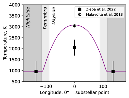
Figure 5: Longitudinal temperature profile at the surface of K2-141 b. See text for details.

The longitudinal temperature profile shows a maximum temperature of $\sim 3080$ K at the substellar point (Fig. 5), in close agreement with [54]. The dayside generally is characterized by temperatures above 1700 K. A penumbral region extends between (-)90° and $\sim$ (-)115°. In this region, temperature drops from $\sim$ 1700 K down to $\sim$ 950 K, the value assumed for the nightside. Given the liquidus temperature of most alumino-silicate rocks, we expect extended melting on the dayside, and magma ocean solidification in the penumbral region.

To examine the effect of composition on viscosity, we consider three different compositional scenarios for the magma ocean: Bulk Silicate Earth (BSE) [95], BSE + 20 % FeO (Fe-rich BSE) and a Type-B CAI composition [96]. The first scenario is an Earth-like case, the second assumes a higher Fe/Si for K2-141 b, and the last one is considered given the high dayside temperatures that may promote a shift of the mantle composition toward a refractory endmember due to evaporation [7]. The three compositions are approximated in simplified systems containing only SiO₂, Al₂O₃, MgO, CaO, and FeO; we did not include the alkalis or volatiles (H and C). We calculated the fractions of crystals, gas and melts as a function of temperature for the three different compositional scenarios using FactSage at atmospheric pressures P_atm of 10^-4, 10^-1 and 1 bar.

We first explore the possible longitudinal profile of evaporation/condensation. FactSage calculations provide equilibrium fractions of gas, melt and solids at high temperatures. Using those calculations, we neglect the potential role of interior convective dynamics that could bring fresh melt out of equilibrium with the gas. Despite this limitation, this approach can provide pieces of understanding regarding the possibility of evaporation and condensation of rock vapor from the magma ocean, assuming local equilibrium (in terms of space and time). Given the longitudinal temperature profile, we calculated the longitude at which the system is comprised of greater than 1% of gas (Table 2). At P_atm = 1 bar, temperatures are not high enough to generate significant outgassing for the present alkali-free compositions. At 10^-1 bar, outgassing starts at longitudes lower than $\sim$ 37° for the BSE and Fe-rich BSE case, and is completely inhibited for the CAI case. At 10^-4 bar, outgassing should occurs at longitudes lower than 70°-80° in the three compositional scenarios.

Patm (bar)	BSE	Fe-rich BSE	CAI
10-4	77	78	72
10-1	36	37	0
1	0	0	0

Table 2: Longitudes (degrees) at which the temperature allows for 1% gas and 99% melt at equilibrium for three compositional scenarios and three different atmospheric pressures P_atm.

Another way of visualizing those results is to use the gas fraction obtained for a given mixture of gas and melt at equilibrium at different P_atm and temperatures as a proxy for the outgassing potential. This assumes that high gas fraction in the equilibrium closed-system case will imply more vigourous outgassing at the surface of the dynamic magma ocean. Reporting the equilibrium gas fraction as a function of longitude shows that a 10^-1 bar atmosphere is expected close to the substellar point (Fig. 6). A lower pressure atmosphere is expected at longitudes above 37°, and up to $\sim$ 78° for a P_atm = 10^-4.

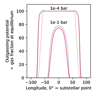
Figure 6: Magma ocean outgassing potential as a function of longitude at the surface of K2-141 b for the BSE (solid lines), Fe-rich BSE (dashed lines) and CAI (dotted lines) compositional scenarios at two different pressures.

The present simple evaluation disregards the presence of volatile and/or alkali elements in the magma. Oxygen fugacity $f$O₂ that may also have an important effect. For instance, recent equilibrium models using both the VapoRock [97] and MAGMA codes [98] show that the total pressure in equilibrium with a volatile-free magma ocean is a strong function of $f$O₂ and temperature. Near 3000 K, surface pressures total 10^-2 bar at the iron-wüstite (IW) buffer, increasing up to $\sim$3.5 bar under reducing conditions ($\Delta$IW = -6). These are calculated on the (reasonable) assumption that the total mass of atmosphere is much lower than the total mass of liquid. In addition, the present calculation disregards atmosphere circulation, which could imply evaporation close to the sub-stellar point and a gradual condensation as gas moves toward the penumbral region [99]. Considering such complexities is outside the scope of this work. However, despite its simplicity, the present analysis corroborates results from the more complete study of [11]. This study suggests that a rock-vapor atmosphere of 10^-1 bar should be present at K2-141 b surface up to $\sim$ 40° longitude. Its pressure will further decrease when going toward the penumbral region. Our present simple calculations agree with such values. Assuming a lateral atmospheric current between the substellar point and the penumbral region, outgassing is thus expected in the 40° region around the substellar point, and rock vapor condensation should occur in the lower pressure regions, between 40° and 90°.

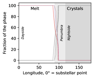
Figure 7: Percent of melt and crystals at surface as a function of longitude for the BSE (solid lines), Fe-rich BSE (dashed lines) and CAI (dotted lines) compositional scenarios. Colored lines are melt fractions and grey lines are crystal fractions.

We now calculate the fractions of melt and crystals the magma ocean contains at surface as a function of longitude (Fig. 7). For simplicity, we neglected the effect of evaporation on the magma ocean composition and assume it acts as a closed system with respect to its elemental composition, at least over the timescales modelled in this work. In all three cases, the magma ocean is fully molten on most of the dayside surface (Fig. 7). Differences only are visible close to the shores, in the penumbral region. The refractory composition (Type B CAI) presents the sharpest transition from fully molten to solid, and the BSE composition has the largest transition region from melt to solid. However, for all compositions we expect a rapid solidification of the magma ocean at the beginning of the penumbral region.

Given variations of melt composition and crystal/liquid fractions, we then calculate the viscosity of the magma using the GP model for the liquid phase. To calculate the effect of the crystals, we use the model of [30] for the liquid-rich magmatic mixture (fraction of crystals $\phi$ lower than 65 %). It includes parameters that account for crystal size and shape distributions as well as maximum packing fraction. For those parameters, we used values determined for peridotite compositions provided in [30]. For crystal-rich magmatic mixtures, we use the model from [100] (at $\phi$ > 65 %). We assume a reference viscosity for the solid mantle of $10^{18}\log_{10}$ Pa$\cdot$s at 1273 K.

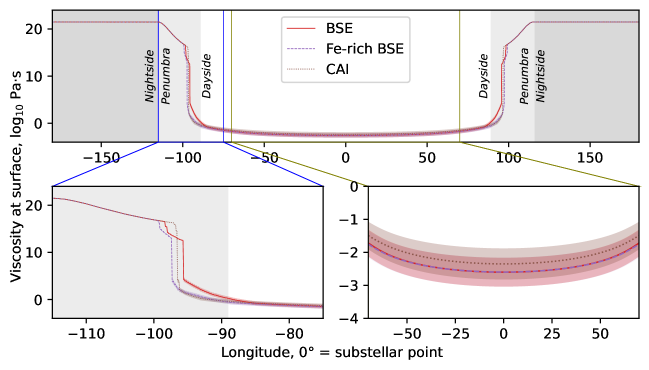
Figure 8: Magma viscosity at surface given longitude, calculated assuming a Earth-like composition (Bulk Silicate Earth, BSE), a Fe-rich composition (Fe-BSE) and a refractory composition (Type B CAI, see [96]). See text for details. Shaded regions on the side of the lines are 95 % confidence intervals.

We observe little variations in the viscosity of the magma between the different considered scenarios (Fig. 8). In most of the dayside, magma viscosity is lower than $10^{-1}$ Pa$\cdot$s. At the substellar point, magma viscosity reaches values of $\sim 10^{-2.3}$ and $\sim 10^{-2.6}$ Pa$\cdot$s for the CAI and BSE/Fe-BSE cases, respectively. Melt composition thus has a small impact ($\sim 0.3$ log units) on the viscosity of the fully molten magma. When going toward the nightside, the earlier appearance of crystals in the BSE case (Fig.7) implies that magma viscosity increases sooner when transitioning from the dayside to the nightside. However, the difference is only of a few degrees compared to the Fe-rich BSE and the CAI refractory compositional scenarios.

Overall, this analysis highlights two points:

• in the high- to very high temperature regimes characteristic of magma oceans on hot super-Earths, temperature exerts the zeroth-order control on magma viscosity, erasing the influence of other factors that usually are critical in Earth-like volcanic systems (e.g. melt composition);

• when temperature decreases, crystallization dictates the rheology of the magma (crystal + liquid), due to combined effects of the presence of solid particles and of the changes it imparts on the residual melt composition. This effect will be important on the shores of magma oceans, but possibly also at depth as crystallization may be favored by the increasing pressure. We do not explore this here because it requires an internal model of the planetary structure that is beyond the scope of this paper.

4.3 K2-141 b: nightside temperature

On the nightside, we expect a solid surface (Fig. 7) with a very high viscosity (Fig. 8). K2-141 b has a very tenuous atmosphere that is unlikely to redistribute heat toward the nightside [11]. Therefore, heat redistribution between the dayside and nightside will be driven by an internal geothermal heat flow. It follows that the nightside surface temperature $T_{s}$ will be controlled by a balance between the geothermal heat flux $Q_{geo}$ and the radiative surface heat flux $Q_{rad}=\sigma_{B}T_{s}^{4}$, with $\sigma_{B}$ the Stefan-Boltzmann constant. $Q_{geo}$ can be sustained either by horizontal transport of heat from the dayside to the nightside by a thin magma ocean under a lid, or by vertical transport from the interior to the surface by the rocky mantle (potentially partially molten). In the case of horizontal convection, $Q_{geo}$ can be expressed as [101]:

$$Q_{geo}=k\frac{\Delta T}{L}R_{a}^{1/5}\>,$$ (4)

with $k$ the average thermal conductivity, $\Delta T=T_{s}-T_{i}$ with $T_{i}$ the average internal temperature of the molten layer, $L$ the height of the convecting layer, and $R_{a}$ the Rayleigh number equal to

$$R_{a}=\frac{\rho g\alpha\Delta TL^{3}}{D\eta}\>,$$ (5)

where $g$ is the gravity acceleration, and $\rho$, $\alpha$, $D$ and $\eta$ are respectively the average values of density, thermal expansivity, thermal diffusivity and viscosity of the material composing the convecting layer. For vertical convection, two cases can be distinguished: hard and soft convection. In the case of a mantle containing a large fraction of melt (below the rheological threshold at around 60 vol% solids), $R_{a}$ will be very high ($\sim$10³⁰ for an Earth-sized planet) and hard convection should be considered, such that we have [102]:

$$Q_{geo}=0.22k\frac{\Delta T}{L}R_{a}^{2/7}P_{r}^{-1/7}\lambda^{-3/7}\>,$$ (6)

where $P_{r}=\frac{D}{\rho\eta}$ is the Prandtl number and $\lambda$ is the aspect ratio for the mean flow. We assume $\lambda=1$ in the following, following [102]. Now, if the mantle is mostly composed of crystals, it will undergo the rheological transition and $R_{a}$ will decrease significantly. Compared to the fully molten magma ocean, we expect a decrease by approximately 15 orders of magnitude as viscosity drastically increases (Fig. 8). Soft convection should then be considered and the heat flux can be expressed as [102]:

$$Q_{geo}=0.089k\frac{\Delta T}{L}R_{a}^{1/3}\>.$$ (7)

By equating $Q_{geo}$ with $Q_{rad}$, we can calculate the nightside surface temperature by iteration. We performed this for two cases: horizontal and hard convection. We neglect the case of soft convection as it is valid for crystal-rich cases (above the rheological threshold). Actually, in details, equation 7 does not really apply for solid mantle convection and another functional form should be adopted [103]. Here, we neglect this and use the hard convection case to provide an upper limit on $T_{s}$ for crystal-rich cases.

Figure 9 shows the result of the calculation for a convecting layer of 1000 km, in the three cases mentioned previously: BSE, Fe-rich BSE and Type B CAI. For the calculations, we used $\rho\sim\mathcal{N}(4000,\,400^{2})$, $\alpha\sim\mathcal{N}(6e-5,\,6e-6^{2})$, $D\sim\mathcal{N}(5e-7,\,2e-7^{2})$, $C_{p}\sim\mathcal{N}(1500,\,150^{2})$ following experimental values and calculations from [104, 105, 106, 107, 108]. We neglect variations of those properties with melt composition as their influence is minimal because they do not vary by several orders of magnitude. On the contrary, the convecting layer viscosity can vary by up to 27 orders of magnitude as a function of temperature and magma crystal content (Fig. 8). In particular, the influence of crystallization on melt viscosity is paramount, and unfortunately one uncertainty remains: the volumetric fraction of crystals at which the rheological threshold, $\phi_{c}$, occurs. $\phi_{c}$ is usually taken to be at a solid fraction of 0.60 [109]. Below $\phi_{c}$, the convecting layer has the rheological behavior of a crystal-bearing liquid. Calculated magma viscosities are lower than $10^{6}$ Pa$\cdot$s and the magma ocean $R_{a}$ will be above $10^{25}$. However, above $\phi_{c}=0.60$, the rheological behavior changes. The convecting layer adopts the rheological behavior of a partly-molten solid, magma viscosity largely increases and $R_{a}$ will significantly decrease. The value of $\phi_{c}$ is thus critical. It varies significantly with crystal size and shape [30, 110, 31, 111, 109]. Here, to take into account of the uncertainty surrounding the value of $\phi_{c}$ in the different scenarios, we assume for $\phi_{c}$ a normal distribution with a mean of 0.6 and a standard deviation of 0.06, i.e. we assume a 10% error on $\phi_{c}$.

Using the normal distributions for the different parameters, we re-calculated the magma viscosity curves and generated the surface temperature versus internal temperature curves for the horizontal convection and hard convection case (Fig. 9). We observe that horizontal convection is not efficient in redistributing the thermal energy (Fig. 9(a)). If this mode is dominant, we do not expect temperatures above 600 K at the nightside surface of a dry exoplanet such as K2-141 b, even in the presence of a molten magma ocean beneath a lid on the nightside. Vertical hard convection is more efficient at providing a sustained geothermal flux (Fig. 9(b)). In this case, the nightside surface can reach temperatures above 400 K if the average internal nightside temperature is above $\sim$ 1600 K. This limit is easily understandable: this corresponds to the temperature at which the compositions studied reach the rheological transition, that is, they are $\sim$ 60 % molten. Above the rheological transition, in the case of a largely molten nightside mantle, the average nightside temperature closely mirrors the average internal nightside temperature.

We finally note that little differences are discernible between the three different melt compositions. The visible difference concerns the onset of the nightside surface temperature rise for a given internal nightside temperature when the latter is around 1600 K. This arises and is due to differences in how the crystallisation sequences between the BSE, Fe-BSE and CAI magma depend on temperature between the melt compositions. In any case, most uncertainties for the determination of the curves shown in figure 9 arise from the uncertainty on $\phi_{c}$. The maximal influence of melt composition can be observed when comparing the endmember cases of fully depolymerized MgSiO₃ and fully polymerized SiO₂ melts (Fig. 9). While the curve for liquid MgSiO₃ closely follows those of the BSE, Fe-rich BSE and Type B CAI cases (except below $\sim$ 1600 K as MgSiO₃ is considered fully molten), a fully polymerized, very viscous SiO₂ liquid mantle will not redistribute efficiently heat to the surface.

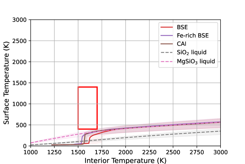
(a)

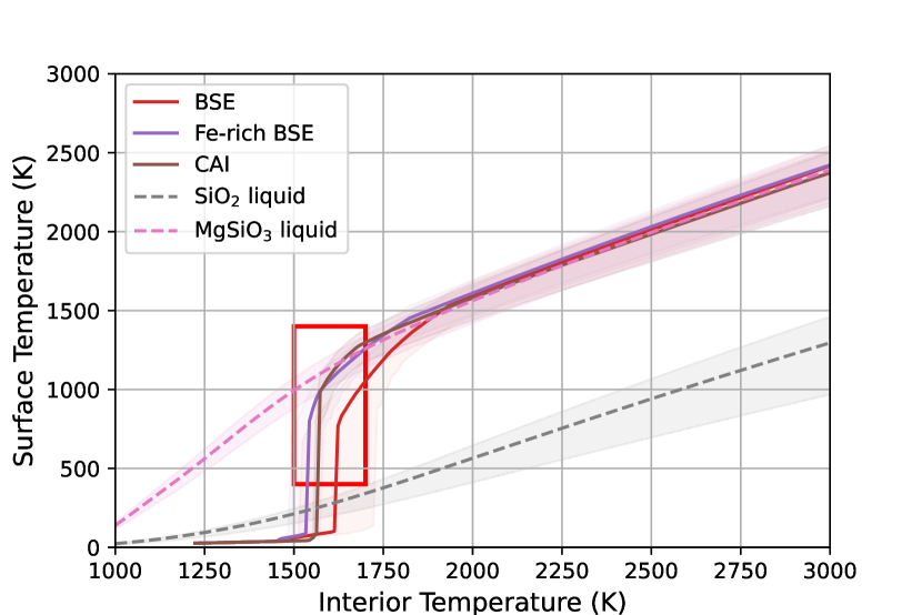
(b)

Figure 9: Average nightside surface temperature as a function of average nightside internal temperature of the convecting layer for two cases: horizontal (a, eq. 4) and hard (b, eq. 6) convections. The red shaded area delimits the temperature range estimated for K2-141 b [11]. The curves are the mean values of 200 models, calculated by sampling the parameter distributions described in the text. Shaded areas around those curves represent the 95% confidence intervals of model predictions.

The present calculations have inherent limitations, such as the absence of any consideration regarding temperature, pressure and associated property gradients. Besides, while horizontal convection appears unlikely to efficiently transport heat, the reality may be more complex as this mode is not well understood in the case of the laterally varying surface heating that applies for USP lava planets [14]. Despite such limitations, the present calculations yield an important conclusion. For sustaining a nightside temperature above 400 K without atmospheric redistribution, as suggested for K2-141 b [11], a portion of the nightside mantle should be partly molten. From figure 9, we estimate that this partly molten mantle portion should have a melt fraction at or slightly above 0.4.

5 Conclusion

In this paper, we presented a new database and its use to train machine learning models to predict the viscosity of water-bearing alumino-phospho-silicate melts as a function of their chemical composition, temperature and pressure. Greybox artificial neural networks produce good results. Their predictions can further be refined using a Gaussian Process (GP). This GP model achieves very good predictive accuracy (RMSE $\sim 0.4\log_{10}$ Pa$\cdot$s), and further yields confidence intervals on predictions. In its current implementation, the GP model is able to predict the viscosity of very various melts, from pure H₂O, SiO₂, P₂O₅, Al₂O₃ to multicomponent magmatic, industrial and laboratory phospho-alumino-silicate melts. Pressure effects can be reproduced up to 30 GPa for compositions like peridotite or MgSiO₃. Therefore, the GP model allows calculating the properties of magmas in a wide variety of scenarios, including (water-rich) magmatic systems in subduction regions, alkali-rich intraplate volcanism, magma oceans, extra-terrestrial volcanisms involving compositions far from the Earth trends. Glass manufacturing may also use this model to calculate melt viscosity in glass-forming furnaces, with potential applications in furnace or compositional design for ensuring energy efficient and environmentally effective production of glass.

The present model has the limitation of many machine learning algorithms: it is an interpolative model that does not behave well when asked to extrapolate to conditions and/or compositions outside its training range. Fortunately, this can be checked: in case of doubt, querying values from a few different GP models allows assessing the quality of predictions. This can be done using the open source, free gpvisc Python library that makes available the models and source code [73].

We used the GP model to estimate the viscosity of a magma ocean at the surface of the dry USP exoplanet K2-141 b, given three different compositional scenarios: bulk silicate Earth BSE, BSE + 20 mol% Fe, and refractory (type B CAI). Assuming a null bond albedo, calculation of surface temperature indicates that K2-141 b dayside is fully molten in all three scenarios. On the dayside, the extreme temperatures generally dictate melt viscosity, and other parameters such as melt composition are secondary. Phase calculations indicate that a tenuous atmosphere with a pressure of $10^{-1}$ bar may be present in a 40° around the substellar point, in agreement with [11]. When going to higher longitudes, the atmospheric pressure is expected to drop to very low values. When reaching the penumbral region at a longitude of 90°, magma viscosity increases rapidly as magma ocean solification proceeds. The composition of the magma slightly affects the position of the shores, but this effect is limited (a few degrees). In the nightside region, surface is expected to be solid. However, estimated nighside temperatures above 400 K [11] suggest that the mantle below the surface is partly molten and feeds the geothermal flux through vertical convection.

Funding

This study was supported by the LabEx UnivEarthS, ANR-10-LABX-0023 and ANR-18-IDEX-0001.

Author contributions

Study design: all authors. Database construction: CF, CLL. Machine learning modelling: CLL, CF. Phase diagram calculations: PS. Temperature and fluid dynamics calculations: CEB, CLL. Manuscript draft: CLL. Manuscrit redaction: all authors.

Competing interests

Authors declare no competing interests.

Materials & Correspondence

The viscosity database is available at [57]. The computer code to reproduce the results of this study is available as a Python library at the web address https://github.com/charlesll/gpvisc and on Zenodo [73]. Correspondence can be addressed to the corresponding author.

References

- [1] S. Labrosse, J. W. Hernlund, and N. Coltice, “A crystallizing dense magma ocean at the base of the Earth’s mantle,” Nature, vol. 450, no. 866-869, 2007.
- [2] D. C. Rubie, F. Nimmo, and H. J. Melosh, “Formation of Earth’s Core,” in Treatise on Geophysics (G. Schubert, ed.), pp. 51–90, Amsterdam: Elsevier, 2007.
- [3] L. T. Elkins-Tanton, “Magma Oceans in the Inner Solar System,” Annual Review of Earth and Planetary Sciences, vol. 40, no. 1, pp. 113–139, 2012.
- [4] P. A. Sossi, A. D. Burnham, J. Badro, A. Lanzirotti, M. Newville, and H. S. O’Neill, “Redox state of Earth’s magma ocean and its Venus-like early atmosphere,” Science Advances, vol. 6, no. 48, p. eabd1387, 2020.
- [5] F. Gaillard, F. Bernadou, M. Roskosz, M. A. Bouhifd, Y. Marrocchi, G. Iacono-Marziano, M. Moreira, B. Scaillet, and G. Rogerie, “Redox controls during magma ocean degassing,” Earth and Planetary Science Letters, vol. 577, p. 117255, Jan. 2022.
- [6] K.-H. Chao, R. deGraffenried, M. Lach, W. Nelson, K. Truax, and E. Gaidos, “Lava Worlds: From Early Earth to Exoplanets,” Geochemistry, vol. 81, p. 125735, May 2021.
- [7] A. Léger, O. Grasset, B. Fegley, F. Codron, A. F. Albarede, P. Barge, R. Barnes, P. Cance, S. Carpy, F. Catalano, C. Cavarroc, O. Demangeon, S. Ferraz-Mello, P. Gabor, J. M. Grießmeier, J. Leibacher, G. Libourel, A. S. Maurin, S. N. Raymond, D. Rouan, B. Samuel, L. Schaefer, J. Schneider, P. A. Schuller, F. Selsis, and C. Sotin, “The extreme physical properties of the CoRoT-7b super-Earth,” Icarus, vol. 213, pp. 1–11, May 2011.
- [8] B.-O. Demory, M. Gillon, J. de Wit, N. Madhusudhan, E. Bolmont, K. Heng, T. Kataria, N. Lewis, R. Hu, J. Krick, V. Stamenković, B. Benneke, S. Kane, and D. Queloz, “A map of the large day–night temperature gradient of a super-Earth exoplanet,” Nature, vol. 532, pp. 207–209, Apr. 2016.
- [9] B.-O. Demory, M. Gillon, N. Madhusudhan, and D. Queloz, “Variability in the super-Earth 55 Cnc e,” Monthly Notices of the Royal Astronomical Society, vol. 455, pp. 2018–2027, Jan. 2016.
- [10] S. J. Mercier, L. Dang, A. Gass, N. B. Cowan, and T. J. Bell, “Revisiting the Iconic Spitzer Phase Curve of 55 Cancri e: Hotter Dayside, Cooler Nightside and Smaller Phase Offset,” The Astronomical Journal, vol. 164, p. 204, Nov. 2022.
- [11] S. Zieba, M. Zilinskas, L. Kreidberg, T. G. Nguyen, Y. Miguel, N. B. Cowan, R. Pierrehumbert, L. Carone, L. Dang, M. Hammond, T. Louden, R. Lupu, L. Malavolta, and K. B. Stevenson, “K2 and Spitzer phase curves of the rocky ultra-short-period planet K2-141 b hint at a tenuous rock vapor atmosphere,” Astronomy & Astrophysics, vol. 664, p. A79, Aug. 2022.
- [12] S. Charnoz, A. Falco, P. Tremblin, P. Sossi, R. Caracas, and P.-O. Lagage, “The effect of a small amount of hydrogen in the atmosphere of ultrahot magma-ocean planets: Atmospheric composition and escape,” Astronomy & Astrophysics, vol. 674, p. A224, June 2023.
- [13] A. Salvador and H. Samuel, “Convective outgassing efficiency in planetary magma oceans: Insights from computational fluid dynamics,” Icarus, vol. 390, p. 115265, Jan. 2023.
- [14] T. G. Meier, D. J. Bower, T. Lichtenberg, M. Hammond, and P. J. Tackley, “Interior dynamics of super-Earth 55 Cancri e,” Astronomy & Astrophysics, vol. 678, p. A29, Oct. 2023.
- [15] C.-É. Boukaré, D. Lemasquerier, N. Cowan, H. Samuel, and J. Badro, “Lava planets interior dynamics govern the long-term evolution of their magma oceans,” Aug. 2023.
- [16] K. Heng, “The Transient Outgassed Atmosphere of 55 Cancri e,” The Astrophysical Journal Letters, vol. 956, p. L20, Oct. 2023.
- [17] A. Falco, P. Tremblin, S. Charnoz, R. J. Ridgway, and P.-O. Lagage, “Hydrogenated atmospheres of lava planets: Atmospheric structure and emission spectra.,” Astronomy & Astrophysics, vol. in press.
- [18] N. Madhusudhan, K. K. M. Lee, and O. Mousis, “A POSSIBLE CARBON-RICH INTERIOR IN SUPER-EARTH 55 Cancri e,” The Astrophysical Journal, vol. 759, p. L40, Nov. 2012.
- [19] A. Tsiaras, M. Rocchetto, I. P. Waldmann, O. Venot, R. Varley, G. Morello, M. Damiano, G. Tinetti, E. J. Barton, S. N. Yurchenko, and J. Tennyson, “DETECTION OF AN ATMOSPHERE AROUND THE SUPER-EARTH 55 CANCRI E,” The Astrophysical Journal, vol. 820, p. 99, Mar. 2016.
- [20] I. Angelo and R. Hu, “A Case for an Atmosphere on Super-Earth 55 Cancri e,” The Astronomical Journal, vol. 154, p. 232, Nov. 2017.
- [21] C.-É. Boukaré, H. Samuel, and J. Badro, “Beyond 1D Magma Ocean Models,” vol. 2022, pp. DI32A–08, Dec. 2022.
- [22] R. Hu, A. Bello-Arufe, M. Zhang, K. Paragas, M. Zilinskas, C. van Buchem, M. Bess, J. Patel, Y. Ito, M. Damiano, M. Scheucher, A. V. Oza, H. A. Knutson, Y. Miguel, D. Dragomir, A. Brandeker, and B.-O. Demory, “A secondary atmosphere on the rocky Exoplanet 55 Cancri e,” Nature, pp. 1–2, May 2024.
- [23] G. S. Fulcher, “Analysis of Recent Measurements of the Viscosity of Glasses,” Journal of the American Ceramic Society, vol. 8, no. 6, pp. 339–355, 1925.
- [24] I. Friedman, W. Long, and R. L. Smith, “Viscosity and water content of rhyolite glass,” Journal of Geophysical Research, vol. 68, no. 24, pp. 6523–6535, 1963.
- [25] G. Urbain, Y. Bottinga, and P. Richet, “Viscosity of liquid silica, silicates and alumino-silicates,” Geochimica et Cosmochimica Acta, vol. 46, pp. 1061–1072, June 1982.
- [26] P. Richet, A.-M. Lejeune, F. Holtz, and J. Roux, “Water and the viscosity of andesite melts,” Chemical Geology, vol. 128, pp. 185–197, June 1996.
- [27] A.-M. Lejeune and P. Richet, “Rheology of crystal-bearing silicate melts: An experimental study at high viscosities,” Journal of Geophysical Research, vol. 100, no. 4215-4229, 1995.
- [28] D. Giordano, J. K. Russell, and D. B. Dingwell, “Viscosity of magmatic liquids: A model,” Earth and Planetary Science Letters, vol. 271, pp. 123–134, July 2008.
- [29] M. Manga, J. Castro, K. V. Cashman, and M. Loewenberg, “Rheology of bubble-bearing magmas,” Journal of Volcanology and Geothermal Research, vol. 87, pp. 15–28, 1998.
- [30] A. Costa, L. Caricchi, and N. Bagdassarov, “A model for the rheology of particle-bearing suspensions and partially molten rocks,” Geochemistry Geophysics Geosystems, vol. 10, no. 3, pp. 1–13, 2009.
- [31] H. Mader, E. Llewellin, and S. Mueller, “The rheology of two-phase magmas: A review and analysis,” Journal of Volcanology and Geothermal Research, vol. 257, pp. 135–158, May 2013.
- [32] J. K. Russell, K.-U. Hess, and D. B. Dingwell, “Models for Viscosity of Geological Melts,” Reviews in Mineralogy and Geochemistry, vol. 87, pp. 841–885, May 2022.
- [33] Y. Bottinga and D. F. Weill, “The viscosity of magmatic silicate liquids: A model for calculation,” American Journal of Science, vol. 272, pp. 438–475, 1972.
- [34] H. R. Shaw, “Viscosities of magmatic silicate liquids; an empirical method of prediction,” American Journal of Science, vol. 272, pp. 870–893, 1972.
- [35] E. S. Persikov, “The viscosity of magmatic liquids : Experiment, generalized patterns. A model for calculation and prediction. Applications.,” Advances in Physical Geochemistry, vol. 9, pp. 1–40, 1991.
- [36] H. Hui and Y. Zhang, “Toward a general viscosity equation for natural anhydrous and hydrous silicate melts,” Geochimica et Cosmochimica Acta, vol. 71, no. 2, pp. 403–416, 2007.
- [37] E. S. Persikov and P. G. Bukhtiyarov, “Interrelated structural chemical model to predict and calculate viscosity of magmatic melts and water diffusion in a wide range of compositions and T-P parameters of the Earth’s crust and upper mantle,” Russian Geology and Geophysics, vol. 50, pp. 1079–1090, Dec. 2009.
- [38] X. Duan, “A model for calculating the viscosity of natural iron-bearing silicate melts over a wide range of temperatures, pressures, oxygen fugacites, and compositions,” American Mineralogist, vol. 99, pp. 2378–2388, Nov. 2014.
- [39] K. U. Hess and D. D. Dingwell, “Viscosities of hydrous leucogranitic melts: A non-Arrhenian model,” American Mineralogist, vol. 81, no. 9-10, pp. 1297–1300, 1996.
- [40] F. Vetere, H. Behrens, F. Holtz, and D. Neuville, “Viscosity of andesitic melts—new experimental data and a revised calculation model,” Chemical Geology, vol. 228, pp. 233–245, Apr. 2006.
- [41] W. L. Romine and A. G. Whittington, “A simple model for the viscosity of rhyolites as a function of temperature, pressure and water content,” Geochimica et Cosmochimica Acta, vol. 170, pp. 281–300, Dec. 2015.
- [42] J. K. Russell, K.-U. Hess, and D. B. Dingwell, “Ultramafic Melt Viscosity: A Model,” May 2024.
- [43] A. Sehlke and A. G. Whittington, “The viscosity of planetary tholeiitic melts: A configurational entropy model,” Geochimica et Cosmochimica Acta, vol. 191, pp. 277–299, Oct. 2016.
- [44] C. Le Losq and D. R. Neuville, “Molecular structure, configurational entropy and viscosity of silicate melts: Link through the Adam and Gibbs theory of viscous flow,” Journal of Non-Crystalline Solids, vol. 463, pp. 175–188, May 2017.
- [45] J. K. Russell and D. Giordano, “Modelling configurational entropy of silicate melts,” Chemical Geology, vol. 461, pp. 140–151, 2017.
- [46] K. Starodub, G. Wu, E. Yazhenskikh, M. Müller, A. Khvan, and A. Kondratiev, “An Avramov-based viscosity model for the SiO2-Al2O3-Na2O-K2O system in a wide temperature range,” Ceramics International, vol. 45, pp. 12169–12181, June 2019.
- [47] D. Langhammer, D. Di Genova, and G. Steinle-Neumann, “Modeling Viscosity of Volcanic Melts With Artificial Neural Networks,” Geochemistry, Geophysics, Geosystems, vol. 23, no. 12, p. e2022GC010673, 2022.
- [48] A. Tandia, M. C. Onbasli, and J. C. Mauro, “Machine Learning for Glass Modeling,” in Springer Handbook of Glass (J. D. Musgraves, J. Hu, and L. Calvez, eds.), Springer Handbooks, pp. 1157–1192, Cham: Springer International Publishing, 2019.
- [49] D. R. Cassar, “ViscNet: Neural network for predicting the fragility index and the temperature-dependency of viscosity,” Acta Materialia, vol. 206, p. 116602, 2021.
- [50] C. Le Losq, A. P. Valentine, B. O. Mysen, and D. R. Neuville, “Structure and properties of alkali aluminosilicate glasses and melts: Insights from deep learning,” Geochimica et Cosmochimica Acta, vol. 314, pp. 27–54, Dec. 2021.
- [51] D. R. Cassar, “GlassNet: A multitask deep neural network for predicting many glass properties,” Mar. 2023.
- [52] C. Le Losq and B. Baldoni, “Machine learning modeling of the atomic structure and physical properties of alkali and alkaline-earth aluminosilicate glasses and melts,” Journal of Non-Crystalline Solids, vol. 617, p. 122481, Oct. 2023.
- [53] T. G. Nguyen, N. B. Cowan, A. Banerjee, and J. E. Moores, “Modelling the atmosphere of lava planet K2-141b: Implications for low- and high-resolution spectroscopy,” Monthly Notices of the Royal Astronomical Society, vol. 499, pp. 4605–4612, Dec. 2020.
- [54] L. Malavolta, A. W. Mayo, T. Louden, V. M. Rajpaul, A. S. Bonomo, L. A. Buchhave, L. Kreidberg, M. H. Kristiansen, M. Lopez-Morales, A. Mortier, A. Vanderburg, A. Coffinet, D. Ehrenreich, C. Lovis, F. Bouchy, D. Charbonneau, D. R. Ciardi, A. C. Cameron, R. Cosentino, I. J. M. Crossfield, M. Damasso, C. D. Dressing, X. Dumusque, M. E. Everett, P. Figueira, A. F. M. Fiorenzano, E. J. Gonzales, R. D. Haywood, A. Harutyunyan, L. Hirsch, S. B. Howell, J. A. Johnson, D. W. Latham, E. Lopez, M. Mayor, G. Micela, E. Molinari, V. Nascimbeni, F. Pepe, D. F. Phillips, G. Piotto, K. Rice, D. Sasselov, D. Ségransan, A. Sozzetti, S. Udry, and C. Watson, “An Ultra-short Period Rocky Super-Earth with a Secondary Eclipse and a Neptune-like Companion around K2-141,” The Astronomical Journal, vol. 155, p. 107, Mar. 2018.
- [55] O. Barragán, D. Gandolfi, F. Dai, J. Livingston, C. M. Persson, T. Hirano, N. Narita, S. Csizmadia, J. N. Winn, D. Nespral, J. Prieto-Arranz, A. M. S. Smith, G. Nowak, S. Albrecht, G. Antoniciello, A. B. Justesen, J. Cabrera, W. D. Cochran, H. Deeg, P. Eigmuller, M. Endl, A. Erikson, M. Fridlund, A. Fukui, S. Grziwa, E. Guenther, A. P. Hatzes, D. Hidalgo, M. C. Johnson, J. Korth, E. Palle, M. Patzold, H. Rauer, Y. Tanaka, and V. V. Eylen, “K2-141 b - A 5-M super-Earth transiting a K7 V star every 6.7 h,” Astronomy & Astrophysics, vol. 612, p. A95, Apr. 2018.
- [56] A. Borisov, H. Behrens, and F. Holtz, “Ferric/ferrous ratio in silicate melts: A new model for 1 atm data with special emphasis on the effects of melt composition,” Contributions to Mineralogy and Petrology, vol. 173, p. 98, Dec. 2018.
- [57] C. Ferraina, B. Baldoni, and C. Le Losq, “Silicate melt viscosity database for gpvisc,” IPGP Research Collection, 2024.
- [58] D. R. Cassar, “Drcassar/glasspy: GlassPy 0.3.” Zenodo, July 2020.
- [59] F. Pedregosa, G. Varoquaux, A. Gramfort, V. Michel, B. Thirion, O. Grisel, M. Blondel, P. Prettenhofer, R. Weiss, V. Dubourg, et al., “Scikit-learn: Machine learning in Python,” Journal of Machine Learning Research, vol. 12, no. Oct, pp. 2825–2830, 2011.
- [60] I. Goodfellow, Y. Bengio, and A. Courville, Deep Learning. MIT Press, 2016.
- [61] K. P. Murphy, Machine Learning: A Probabilistic Perspective. Cambridge, Massachusetts: The MIT Press, 2012.
- [62] D. Langhammer, D. Di Genova, and G. Steinle-Neumann, “Modeling the Viscosity of Anhydrous and Hydrous Volcanic Melts,” Geochemistry, Geophysics, Geosystems, vol. 22, Aug. 2021.
- [63] J. K. Russell, D. Giordano, and D. B. Dingwell, “High-temperature limits on viscosity of non-Arrhenian silicate melts,” American Mineralogist, vol. 88, no. 8-9, pp. 1390–1394, 2003.
- [64] C. Le Losq, B. Baldoni, and A. Valentine, “Charlesll/i-melt: I-melt v2.0.0.” Zenodo, Apr. 2023.
- [65] C. E. Rasmussen and C. K. I. Williams, Gaussian Processes for Machine Learning. Adaptive Computation and Machine Learning, Cambridge, Mass.: MIT Press, 3. print ed., 2006.
- [66] M. Ziatdinov, A. Ghosh, and S. V. Kalinin, “Physics makes the difference: Bayesian optimization and active learning via augmented Gaussian process,” Aug. 2021.
- [67] J. Zhang, C. Liu, and R. X. Gao, “Physics-guided Gaussian process for HVAC system performance prognosis,” Mechanical Systems and Signal Processing, vol. 179, p. 109336, Nov. 2022.
- [68] X. Glorot, A. Bordes, and Y. Bengio, “Deep sparse rectifier neural networks,” in International Conference on Artificial Intelligence and Statistics, pp. 315–323, 2011.
- [69] A. Paszke, S. Gross, F. Massa, A. Lerer, J. Bradbury, G. Chanan, T. Killeen, Z. Lin, N. Gimelshein, L. Antiga, A. Desmaison, A. Kopf, E. Yang, Z. DeVito, M. Raison, A. Tejani, S. Chilamkurthy, B. Steiner, L. Fang, J. Bai, and S. Chintala, “PyTorch: An Imperative Style, High-Performance Deep Learning Library,” Advances in Neural Information Processing Systems, vol. 32, pp. 8026–8037, 2019.
- [70] D. Hendrycks and K. Gimpel, “Gaussian Error Linear Units (GELUs),” arXiv:1606.08415 [cs], July 2020.
- [71] N. Srivastava, G. Hinton, A. Krizhevsky, I. Sutskever, and R. Salakhutdinov, “Dropout: A Simple Way to Prevent Neural Networks from Overfitting,” Journal of Machine Learning Research, vol. 15, pp. 1929–1958, 2014.
- [72] J. R. Gardner, G. Pleiss, D. Bindel, K. Q. Weinberger, and A. G. Wilson, “GPyTorch: Blackbox Matrix-Matrix Gaussian Process Inference with GPU Acceleration,” June 2021.
- [73] C. Le Losq, C. Ferraina, P. A. Sossi, and C.-E. Boukaré, “charlesll/gpvisc,” Zenodo, 2024.
- [74] G. Wu, E. Yazhenskikh, K. Hack, E. Wosch, and M. Müller, “Viscosity model for oxide melts relevant to fuel slags. Part 1: Pure oxides and binary systems in the system SiO2–Al2O3–CaO–MgO–Na2O–K2O,” Fuel Processing Technology, vol. 137, pp. 93–103, Sept. 2015.
- [75] C. Le Losq, B. Baldoni, A. P. Valentine, and D. R. Neuville, “Modeling the properties of melts along calc-alkaline and alkaline magmatic differentiation trends using deep learning,” in American Geophysical Union Fall Meeting, Dec. 2021.
- [76] A. Sipp, Y. Bottinga, and P. Richet, “New high viscosity data for 3D network liquids and new correlations between old parameters,” Journal of Non-Crystalline Solids, vol. 288, pp. 166–174, 2001.
- [77] W. Hummel and J. Arndt, “Variation of viscosity with temperature and composition in the plagioclase system,” Contributions to Mineralogy and Petrology, vol. 90, no. 1, pp. 83–92, 1985.
- [78] C. M. Scarfe, D. J. Cronin, J. T. Wenzel, and D. A. Kauffman, “Viscosity-temperature relationships at 1 atm in the system diopside-anorthite,” American Mineralogist, vol. 68, pp. 1083–1088, 1983.
- [79] M. Solvang, Y. Z. Yue, S. L. Jensen, and D. B. Dingwell, “Rheological and thermodynamic behaviors of different calcium aluminosilicate melts with the same non-bridging oxygen content,” Journal of Non-Crystalline Solids, vol. 336, pp. 179–188, May 2004.
- [80] M. Brearley, J. E. Jr. Dickinson, and C. M. Scarfe, “Pressure dependence of melt viscosities on the join diopside-albite,” Geochimica et Cosmochimica Acta, vol. 50, pp. 2563–2570, 1986.
- [81] I. Kushiro, “Viscosity and structural changes of albite (NaAlSi3O8) melt at high pressures,” Earth and Planetary Science Letters, vol. 41, pp. 87–90, 1978.
- [82] S. Mori, E. Ohtani, and A. Suzuki, “Viscosity of the albite melt to 7 GPa at 2000 K,” Earth and Planetary Science Letters, vol. 175, pp. 87–92, Jan. 2000.
- [83] B. Cochain, C. Sanloup, C. Leroy, and Y. Kono, “Viscosity of mafic magmas at high pressures,” Geophysical Research Letters, vol. 44, p. 2016GL071600, Jan. 2017.
- [84] C. Liebske, B. Schmickler, H. Terasaki, B. Poe, A. Suzuki, K. Funakoshi, R. Ando, and D. Rubie, “Viscosity of peridotite liquid up to 13 GPa: Implications for magma ocean viscosities,” Earth and Planetary Science Letters, vol. 240, pp. 589–604, Dec. 2005.
- [85] L. Xie, A. Yoneda, T. Katsura, D. Andrault, Y. Tange, and Y. Higo, “Direct Viscosity Measurement of Peridotite Melt to Lower-Mantle Conditions: A Further Support for a Fractional Magma-Ocean Solidification at the Top of the Lower Mantle,” Geophysical Research Letters, vol. 48, no. 19, p. e2021GL094507, 2021.
- [86] H. Behrens and F. Schulze, “Pressure dependence of melt viscosity in the system NaAlSi 3 O 8 -CaMgSi 2 O 6,” American Mineralogist, vol. 88, pp. 1351–1363, Aug. 2004.
- [87] Y. Bottinga and P. Richet, “Silicate melts: The “anomalous” pressure dependence of the viscosity,” Geochimica et Cosmochimica Acta, vol. 59, pp. 2725–2731, July 1995.
- [88] R. Caracas, “The thermal equation of state of the magma Ocean,” Earth and Planetary Science Letters, vol. 637, p. 118724, July 2024.
- [89] S. K. Bajgain, A. W. Ashley, M. Mookherjee, D. B. Ghosh, and B. B. Karki, “Insights into magma ocean dynamics from the transport properties of basaltic melt,” Nature Communications, vol. 13, p. 7590, Dec. 2022.
- [90] D. Huang, Y. Li, and M. Murakami, “Low Viscosity of Peridotite Liquid: Implications for Magma Ocean Dynamics,” Geophysical Research Letters, vol. 51, no. 7, p. e2023GL107608, 2024.
- [91] L. Dang, N. B. Cowan, M. Hammond, L. Kreidberg, R. Lupu, Y. Miguel, G. Nguyen, R. Pierrehumbert, S. Zieba, and M. Zilinskas, “A Hell of a Phase Curve: Mapping the Surface and Atmosphere of a Lava Planet K2-141b,” JWST Proposal. Cycle 1, p. 2347, Mar. 2021.
- [92] J. L. Carter, R. D. Perera, and M. J. Way, “Hyper Illumination of Exoplanets: Analytical and Numerical Approaches,” The Astronomical Journal, vol. 167, p. 222, Apr. 2024.
- [93] J. Carter, “Carterphysicslabs/ExoHype: Initial.” Zenodo, Jan. 2024.
- [94] Z. Essack, S. Seager, and M. Pajusalu, “Low-albedo Surfaces of Lava Worlds,” The Astrophysical Journal, vol. 898, p. 160, Aug. 2020.
- [95] H. Palme and H. St. C. O’Neill, “3.1 - Cosmochemical Estimates of Mantle Composition,” in Treatise on Geochemistry (Second Edition) (H. D. Holland and K. K. Turekian, eds.), pp. 1–39, Oxford: Elsevier, 2014.
- [96] E. Stolper and J. M. Paque, “Crystallization sequences of Ca-Al-rich inclusions from Allende: The effects of cooling rate and maximum temperature,” Geochimica et Cosmochimica Acta, vol. 50, pp. 1785–1806, Aug. 1986.
- [97] A. S. Wolf, N. Jäggi, P. A. Sossi, and D. J. Bower, “VapoRock: Thermodynamics of Vaporized Silicate Melts for Modeling Volcanic Outgassing and Magma Ocean Atmospheres,” The Astrophysical Journal, vol. 947, p. 64, Apr. 2023.
- [98] F. L. Seidler, P. A. Sossi, and S. L. Grimm, “Impact of oxygen fugacity on atmospheric structure and emission spectra of ultra hot rocky exoplanets,” Aug. 2024.
- [99] E. S. Kite, B. F. Jr, L. Schaefer, and E. Gaidos, “ATMOSPHERE-INTERIOR EXCHANGE ON HOT, ROCKY EXOPLANETS,” The Astrophysical Journal, vol. 828, p. 80, Sept. 2016.
- [100] T. Scott and D. L. Kohlstedt, “The effect of large melt fraction on the deformation behavior of peridotite,” Earth and Planetary Science Letters, vol. 246, pp. 177–187, June 2006.
- [101] G. O. Hughes and R. W. Griffiths, “Horizontal Convection,” Annual Review of Fluid Mechanics, vol. 40, pp. 185–208, Jan. 2008.
- [102] V. S. Solomatov, “Fluid Dynamics of a Terrestrial Magma Ocean,” in Origin of the Earth and Moon, pp. 323–338, Tucson: AZ: University of Arizona Press, canup r.m. and righter k. ed., Jan. 2000.
- [103] V. Solomatov, “Magma Oceans and Primordial Mantle Differentiation,” in Treatise on Geophysics, pp. 81–104, Elsevier, 2015.
- [104] R. Eriksson, M. Hayashi, and S. Seetharaman, “Thermal Diffusivity Measurements of Liquid Silicate Melts,” International Journal of Thermophysics, vol. 24, no. 3, pp. 785–797, 2003.
- [105] B. Gibert, U. Seipold, A. Tommasi, and D. Mainprice, “Thermal diffusivity of upper mantle rocks: Influence of temperature, pressure, and the deformation fabric,” Journal of Geophysical Research: Solid Earth, vol. 108, no. B8, 2003.
- [106] A. Suzuki, E. Ohtani, and T. Kato, “Density and thermal expansion of a peridotite melt at high pressure,” Physics of the Earth and Planetary Interiors, vol. 107, pp. 53–61, Apr. 1998.
- [107] P. Richet and Y. Bottinga, “Heat capacity of aluminum-free liquid silicates,” Geochimica et Cosmochimica Acta, vol. 49, pp. 471–486, Feb. 1985.
- [108] C. Le Losq and B. Baldoni, “Machine learning modeling of the atomic structure and physical properties of alkali and alkaline-earth aluminosilicate glasses and melts,” Apr. 2023.
- [109] S. Kolzenburg, M. O. Chevrel, and D. B. Dingwell, “Magma / Suspension Rheology,” Reviews in Mineralogy and Geochemistry, vol. 87, pp. 639–720, May 2022.
- [110] A. Vona, C. Romano, D. B. Dingwell, and D. Giordano, “The rheology of crystal-bearing basaltic magmas from Stromboli and Etna,” Geochimica et Cosmochimica Acta, vol. 75, no. 11, pp. 3214–3236, 2011.
- [111] J. Klein, S. P. Mueller, and J. M. Castro, “The Influence of Crystal Size Distributions on the Rheology of Magmas: New Insights From Analog Experiments,” Geochemistry, Geophysics, Geosystems, vol. 18, no. 11, pp. 4055–4073, 2017.