GTransPDM: A Graph-embedded Transformer with Positional Decoupling for Pedestrian Crossing Intention Prediction
Abstract
Understanding and predicting pedestrian crossing behavioral intention is crucial for autonomous vehicles driving safety. Nonetheless, challenges emerge when using promising images or environmental context masks to extract various factors for time-series network modeling, causing pre-processing errors or a loss in efficiency. Typically, pedestrian positions captured by onboard cameras are often distorted and do not accurately reflect their actual movements. To address these issues, GTransPDM – a Graph-embedded Transformer with a Position Decoupling Module – was developed for pedestrian crossing intention prediction by leveraging multi-modal features. First, a positional decoupling module was proposed to decompose the pedestrian lateral movement and simulate depth variations in the image view. Then, a graph-embedded Transformer was designed to capture the spatial-temporal dynamics of human pose skeletons, integrating essential factors such as position, skeleton, and ego-vehicle motion. Experimental results indicate that the proposed method achieves 92% accuracy on the PIE dataset and 87% accuracy on the JAAD dataset, with a processing speed of 0.05ms. It outperforms the state-of-the-art in comparison.
I INTRODUCTION
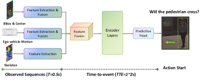
Pedestrians, as vulnerable road users, are a crucial concern in the safe driving of autonomous vehicles (AVs). Accurately understanding and predicting pedestrian behavioral intentions is essential for AVs to make proactive safety decisions [1, 2]. However, pedestrian crossing intention prediction (PCIP) continues to be a challenge in time series classification, where the input comprises a sequence of features derived from sensor data, and the output indicates the probability that a person crosses the road after a given prediction horizon [3], as shown in Fig. 1.
In existing research, RNN and Transformer based approaches are employed to develop time series models with graph neural networks (GNNs) either independently or in conjunction to represent skeletal information [4, 5, 6, 7, 8]. However, the role of skeleton information within the feature fusion paradigm remains controversial in current studies, underscoring the necessity for precise extraction of pose dynamics[9, 10]. To gain a deeper insight into pedestrian crossing behavior, various factors have been explored in existing approaches, showcasing improved performance by incorporating environmental context [11, 12, 13]. However, these methods may lead to errors in image processing, instance mask inference, or become computationally intensive.
Pedestrian trajectories provide valuable insights into pedestrian behavior and have been extensively utilized in PCIP [14, 15, 16, 17]. Yet, since pedestrian positions in the image are relative to the ego-vehicle, this can hinder the models’ ability to accurately identify pedestrian movements in real-world scenarios. Typically, a pedestrian’s lateral shift toward the road is a key indicator of a potential crossing. However, the position may be distorted due to the moving ego-vehicle, making it challenging to pinpoint their actual movements. Moreover, the distance between pedestrians and the ego-vehicle greatly influences the crossing decision [18, 19]. This factor, though critical, has often been neglected in current studies due to the complexity of depth estimation.
To address the above issues, a Graph-embedded Transformer with a Position Decoupling Module (GTransPDM) for PCIP was developed by merging multi-modal features. First, the PDM was introduced to represent pedestrian lateral movements using road-boundary-like reference lines. Then, the area ratio of the bounding boxes was utilized in the PDM to simulate the depth variation between pedestrian and ego-vehicle. Finally, graph convolutional blocks with learnable edge importance were combined with a Transformer-based architecture for PCIP, enabling the consideration of both spatial and temporal variations in human pose skeletons.
The main contributions are summarized as follows.
1) A fast Transformer-based multi-modal fusion framework was proposed to enhance PCIP by integrating data from various sensors.
2) A PDM was proposed to decompose the pedestrians’ lateral movements and simulate the depth variation, to eliminate the positional distortion in on-board image view.
3) A GCN-based embedding was integrated with the Transformer to capture the spatial-temporal dynamics of the human pose skeleton, allowing for accurate modeling of joint interactions and motion patterns.
II Related Work
II-A Pedestrian Intention Prediction in Time-Series Models
Understanding pedestrian crossing behavior is crucial for traffic safety. Before the rise of deep learning, machine learning (ML) methods such as Hidden Markov Models (HMM) [20], Support Vector Machines (SVM) [21, 22], and Random Forests (RF)[8] were used to identify the pedestrian’s action dynamics. However, ML relies on manual feature engineering and it is difficult to handle with high-dimensional and large-scale data, making it less effective in understanding the intricate movement patterns of pedestrians. In recent years, significant attention has been given to deep-learning-based time-series models, particularly variations of RNNs and Transformers [4, 5, 6]. However, RNNs face challenges in capturing long-range dependencies and are less efficient due to their sequential processing. To address these limitations, IntFormer first introduced Transformer encoders to model temporal dynamics [10]. PIT proposed a ViT-based [23] encoder to capture interactions between traffic agents within image frames, and stacking multiple Transformer layers to capture temporal patterns [24]. However, PIT is computationally expensive due to image processing, and IntFormer’s performance still falls short of expectations. This paper enhances these models by introducing positional decoupling and incorporating a graph-embedded Transformer for skeleton dynamics modeling, achieving both lightweight design and higher accuracy.
II-B Skeleton-Based Pedestrian Intention Prediction
Pedestrian skeletal pose offers crucial insights into actions closely associated with crossing behavior. Prior to the emergence of Graph Neural Networks (GNNs) [25], skeletal information was typically used in ML-based approaches, which depended on manually selected joint coordinates, limb angles, and head orientation [8, 14, 26]. Since pedestrian joints and limbs naturally form a graph structure, GNNs and their variants have been extensively adopted for modeling pose dynamics. Notable models include STGCN [27] and GAT [28]. In the PCIP task, skeletal information is often extracted using standalone GNNs [29, 8, 30] or combined with RNNs to capture both spatial and temporal features [5, 9]. Motivated by the success of Transformers [31], some current studies have incorporated self-attention mechanisms into GNNs [32, 33]. However, few studies have explored the combination of GNNs and Transformers in multi-modal fusion paradigm, to the best of our knowledge.
II-C Multi-Feature Fusion for Pedestrian Intention Prediction
Pedestrian crossing behavior is affected by a variety of factors, prompting recent research to concentrate on creating feature fusion methods that incorporate elements, such as pedestrian characteristics (e.g., age, gender) [34], position [16, 35], skeletal pose [29], and environmental factors (e.g., crosswalks, traffic lights) [36, 37]. Pedestrian position, which indicates whether a pedestrian is approaching the road, has emerged as one of the most crucial indicators [14, 15, 16, 17]. However, on-board camera views capture the relative position between the vehicle and the pedestrian, complicating the accurate identification of low-speed pedestrian movements in real-world scenarios. Moreover, the distance between the pedestrian and the ego-vehicle, a key factor in crossing behavior [18, 19], is often overlooked. Furthermore, studies that incorporate environmental context is computationally intensive [4, 5, 6, 7, 8, 24, 38]. In this study, a lightweight network with a PDM is proposed to minimize positional distortion and simulate depth variation, achieving superior performance.
III Methodology
III-A Overview
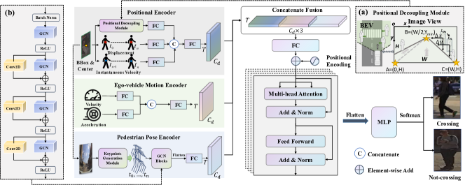
In essence, PICP is a task for predicting action in a binary classification setting, where a sequence of observed frames serves as the input and the output is the probability of crossing after a specified time-to-event (TTE) horizon, as illustrated in Fig. 1. An overview of the proposed framework is presented in Fig. 2.
In the presented framework, the encoding of the network was accomplished by using position, pose, and ego-vehicle motion of the pedestrian across observation frames. Each encoder was referred to as , , and , respectively. In positional encoder, PDM was developed to decompose true lateral movements of the pedestrian and simulate depth changes, which were then integrated with displacement and instantaneous velocity to further present the position shift in image view. Then, the ego vehicle’s motion, indicative of a potential conflict with a pedestrian, was characterized by its speed and acceleration .
In addition, several GCN blocks equipped with residual connections were layered to capture the pedestrian pose dynamics in the spatial domain . Finally, these encoded representations are combined and sent to a Transformer encoder for temporal feature extraction, followed by linking to an MLP head for classification results. As described above, the PCIP problem in this study can be outlined as follows.
| (1) |
III-B Network Encoder
Positional Encoder. In this study, the positional encoder includes displacement , instantaneous velocity , and from the proposed PDM, where and are the absolute center coordinates of the pedestrian bounding box, and . and collectively describe the overall and frame-by-frame displacement of the pedestrian relative to the ego-vehicle.
Some previous studies have treated pedestrian position as absolute coordinates in the image view from the on-board camera [14, 15, 16]. However, when the vehicle is in motion, this can lead to positional distortion, making it difficult for the network to accurately detect pedestrians approaching the road. Moreover, depth is a key factor in crossing behavior but is rarely considered in the existing research. To this end, the PDM was proposed to address the above issue, as shown in Fig. 2 (a). Firstly, two reference lines were set to represent the road boundary coordinates . Then, the disparity between the pedestrian center and the reference line at frame was calculated, namely , where , to indicate position relative to the line of sight. Finally, the area ratio was employed to combine with the position variations in PDM to mimic the depth shift in image view. The whole features in can be represented as:
| (2) |
where: is the bounding box erea at frame . is a factor to magnify the value, was set as .
Each feature in was fed into a fully connected (FC) layer for feature extraction, then concatenated along the channel dimension for feature fusion. Finally, another FC layer was applied for linear projection to produce the output, denoted as:
| (3) |
where: indicates the channel dimension of .
Ego-vehicle Motion Encoder. The motion of the ego-vehicle represents vehicles that are about to conflict with a pedestrian. Thus, speed , and acceleration were utilized simultaneously to describe it. To represent the global , it was calculated as:
| (4) |
where: presents the frames per second depending on video attributes. Furthermore, similar to , the was also encoded and fused by FC layers and concatenate operation:
| (5) |
Skeleton Pose Encoder. The pedestrian skeleton pose reflects the action highly related to the crossing behavior, which can be represented as a graph naturally, where the joints are represented as nodes and limbs as edges . keypoints was utilized, each point is represented as . The adjacency matrix includes the skeleton naturally connections and self-connected matrix. To avoid redundancy with position, each absolute coordinates of keypoint in the image was normalized with its corresponding top-left bounding box coordinates as: , and is the confidence score.
Inspired by [39], four stacked GCN blocks with residual connections were introduced as feature extractors of , as shown in Fig. 2 (b). Furthermore, learnable edge importance was also applied in the network training. The entire process can be denoted as:
| (6) |
where: is the diagonal node degree matrix. and represent the learnable edge importance and feature map in each layer respectively, indicates the ReLU activate function, and is Hadamard product operation. Further, the last layer was flattened to and linear projected as the output of :
| (7) |
where: is the dimension of hidden layers in GCN.
III-C Feature Fusion, Transformer Encoder and Prediction
After encoder layers, the ,,and were generated and concatenated along the channel dimension for feature fusion, with another FC layer for linear projection.
| (8) |
So far, includes the features from all modalities. Benefiting from the multi-head attention (MHA) mechanism in long-range dependencies, Transformer encoder layers [31] were utilized to model on temporal dimension. Firstly, positional encoding (PE) was added in temporal steps:
| (9) |
where: is the index of the embedding dimension . Further, the MHA layer can be denoted as:
| (10) |
With the feature from MHA and layer normalization, a feed-forward network (FFN) with two FC layers was employed, denoted as:
| (11) | ||||
Following the block containing MHA and FFN layers above, a few blocks were sequentially connected for the entire Transformer encoder in temporal modeling. Finally, the output was flattened and an MLP head with a single FC layer was employed for binary classification:
| (12) |
IV Experiments
IV-A Datasets
The effectiveness of the proposed method was evaluated using two large-scale datasets in the context of autonomous driving – JAAD and PIE. JAAD [40] includes 346 short video clips between 5-10 seconds long derived from over 240 hours of recordings collected in the urban of North America and Eastern Europe. PIE [41] contains more than 6 hours of footage captured in the downtown of Toronto, Canada. Both datasets are annotated with the crossing point in time, enabling the TTE calculation. The video frame rate from the two datasets is 30 FPS. Instead of ego-vehicle speed, five ego-vehicle motion states were used in the of JAAD, as velocity data are not available.
The data used in the PIE experiments was split into train, validation (val), and test at a ratio of 0.5:0.1:0.4, with random splitting based on person IDs. For comparison with existing methods (Table I), the performance following the data split in [3] was tested, with 4770, 1332, and 3816 samples in train, val, and test sets respectively. For the JAAD dataset, the JAAD_all subset and adhered to the default data split provided by the benchmark were used, including 8613, 1265, and 6732 sequences for each part. Furthermore, 0.5 second () observations were utilized to predict pedestrian crossing intention after 1-2 seconds (), sampled data based on the sliding window with an overlap of 0.6, 0.8 for PIE and JAAD dataset, respectively.
IV-B Implementation Details
In the network architecture, the dimension of three encoder layers , hidden layers in GCN , and in Transformers are all set to 64. With the concatenate operation in the feature fusion block, the channel dimension of the fused feature is . In the transformer encoder, , 4 attention heads, and 4 stacked layers were applied to extract temporal information. The reference lines in PDM were set to one line between points: and while another between: and , as shown in Fig. 2 (a), where is the minimum of all samples in each dataset. The minor differences in coordinates have little impact on model performance in subsequent experiments, as shown in Table II. The keypoints were offline generated by the pre-trained Alphapose [42], while the additional neck, hip, and body center points were further calculated based on the average of adjacent points.
The cross-entropy loss [43] was utilized for network training. For the PIE dataset, we trained for 32 epochs with a batch size of 128, using the Adam optimizer with an initial learning rate of , and employed the ReduceLROnPlateau scheduler to halve the learning rate if the validation loss do not decrease by over 8 epochs. In JAAD, the AdamW optimizer with a constant learning rate of was applied for 32 epochs training, with a batch size of 64. Additionally, a weight decay of was applied on both datasets to mitigate overfitting. All experiments were conducted on a server equipped with an NVIDIA TITAN X GPU with 12 GB of memory.
| Models | PIE | JAAD | ||||||
|---|---|---|---|---|---|---|---|---|
| Acc | AUC | F1 | P | Ac | AUC | F1 | P | |
| BiPed[44] | 0.91 | 0.90 | 0.85 | 0.82 | 0.83 | 0.79 | 0.60 | 0.52 |
| Pedestrian Graph+ [45] | 0.89 | 0.90 | 0.81 | 0.83 | 0.86 | 0.88 | 0.65 | 0.58 |
| MultiRNN [46] | 0.83 | 0.80 | 0.71 | 0.69 | 0.79 | 0.79 | 0.58 | 0.45 |
| SFRNN [13] | 0.82 | 0.79 | 0.69 | 0.67 | 0.84 | 0.84 | 0.65 | 0.54 |
| SingleRNN [17] | 0.81 | 0.75 | 0.64 | 0.67 | 0.78 | 0.75 | 0.54 | 0.44 |
| PCPA[3] | 0.87 | 0.86 | 0.77 | / | 0.85 | 0.86 | 0.68 | / |
| TrouSPI-Net[47] | 0.88 | 0.88 | 0.80 | 0.73 | 0.85 | 0.73 | 0.56 | 0.57 |
| IntFormer[10] | 0.89 | 0.92 | 0.81 | / | 0.86 | 0.78 | 0.62 | / |
| FF-STP[4] | 0.89 | 0.86 | 0.80 | 0.79 | 0.83 | 0.82 | 0.63 | 0.51 |
| PIT [24] | 0.91 | 0.92 | 0.82 | 0.84 | 0.87 | 0.89 | 0.67 | 0.58 |
| GTransPDM (w/o ) | 0.92 | 0.90 | 0.86 | 0.85 | 0.84 | 0.72 | 0.54 | 0.56 |
| GTransPDM | 0.90 | 0.87 | 0.82 | 0.86 | 0.87 | 0.78 | 0.64 | 0.64 |
IV-C Evaluations
The effectiveness of our method was evaluated using Accuracy, Area Under Curve (AUC), F1 Score, Precision, and Recall, which are commonly used in existing studies. Table I compares our method with recent approaches from the past five years, including Transformer-based IntFormer [10] and PIT [24], the graph-based Pedestrian Graph+[45], and several RNN-based methods. Except BiPed[44] and Pedestrian Graph+ [45], other solutions show the same data splits and configurations as ours, following [3]. Additionally, we trained and tested MultiRNN[46], SingleRNN[17], and SFRNN[13], published before the benchmark released, using the codebase from [3]. While PIT [24] captures traffic agent interactions using a ViT-based [23] network with 16 stacked Transformer layers, incurring high computational costs, our lightweight network achieves superior performance, reaching 0.92 accuracy and 0.86 F1 in PIE using only position and ego-vehicle motion encoders, with 0.86 precision when incorporating the pose encoder. However, as shown in Table I, most PIE metrics are higher without , likely due to the benchmark’s video-based data split, reducing the randomness of pedestrian crossing patterns. To ensure a more balanced comparison, we split the data by pedestrian IDs in later experiments. Regarding JAAD, we achieves 0.87 accuracy and 0.64 precision, surpassing most existing methods.
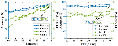
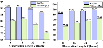
Fig. 3 shows the performance based on different TTE settings, ranging from 0 to 60 frames. A smaller TTE value indicates a shorter prediction interval. In the PIE experiment, we observed that as TTE decreased, the model’s performance improved rapidly. Without a TTE interval (TTE = 0), the accuracy and F1 score reached 99.32% and 98.73%, respectively. However, in the JAAD experiments, the performance improved only when very close to the action start time, mostly because the JAAD_all subset contains a large number of pedestrians who are far away and do not interact with the driver, which confuses the model’s ability to identify crossing behavior that truly influenced by the ego-vehicle. Fig. 4 presents how the observation length influenced model performance. Remarkably, in the PIE dataset, prediction accuracy initially improved and then declined as the observation time extended, whereas in the JAAD dataset, longer observation times consistently resulted in higher accuracy. This is because the PIE contains more diverse pedestrian samples from urban downtown areas, where behavior before crossing can change unpredictably. As a result, extended observation times may lead to misjudgments by the model. In contrast, pedestrian crossing behavior in JAAD is relatively simpler, allowing longer observation periods to more effectively capture pedestrian movement patterns.
We also tested the model’s performance with different reference line coordinates, as shown in Table II. Since the in PDM are only influenced by the line’s slope, we varied the vertical coordinates of points and for testing. With little variation in the line slope, the model’s performance remained less affected.
| PIE | JAAD | |||||
|---|---|---|---|---|---|---|
| Acc | AUC | F1 | Acc | AUC | F1 | |
| 91.21 | 88.13 | 81.61 | 87.43 | 78.16 | 64.00 | |
| 91.24 | 87.70 | 81.42 | 87.25 | 77.81 | 63.46 | |
| 91.16 | 87.65 | 81.29 | 87.36 | 77.74 | 63.52 | |
| Encoders | Choice | ||||
|---|---|---|---|---|---|
| ✓ | ✓ | ✓ | |||
| ✓ | ✓ | ✓ | |||
| ✓ | ✓ | ||||
| Acc | 88.17/84.76 | 84.73/82.52 | 82.19/84.45 | 90.43/84.43 | 91.21/87.43 |
| AUC | 83.63/70.28 | 77.84/50.00 | 71.72/70.29 | 86.36/71.89 | 88.13/78.16 |
| F1 | 75.04/52.41 | 66.78/0.00 | 57.98/52.17 | 79.57/54.16 | 81.61/64.00 |
| Precision | 75.08/57.71 | 68.94/0.00 | 65.81/56.42 | 80.53/55.82 | 80.97/64.11 |
| Choice | ||||||
| ✓ | ✓ | ✓ | ✓ | ✓ | ||
| ✓ | ✓ | ✓ | ✓ | ✓ | ||
| ✓ | ✓ | ✓ | ||||
| ✓ | ||||||
| ✓ | ||||||
| Acc | 89.94/84.12 | 90.07/84.19 | 90.22/82.09 | 90.43/82.75 | 91.21/87.43 | 91.44/84.12 |
| AUC | 86.12/72.16 | 84.73/73.92 | 83.39/73.54 | 87.69/74.08 | 88.13/78.16 | 88.12/72.53 |
| F1 | 78.80/54.22 | 78.08/56.25 | 77.35/54.11 | 80.33/55.19 | 81.61/64.00 | 81.93/54.65 |
| Precision | 78.76/54.66 | 81.92/54.50 | 85.81/49.00 | 78.30/50.57 | 80.97/64.11 | 82.01/54.58 |
| Acc | AUC | F1 | Precision | Recall | ||
|---|---|---|---|---|---|---|
| ✓ | 90.22% | 86.15% | 79.18% | 79.96% | 78.42% | |
| ✓ | 90.60% | 85.52% | 79.29% | 83.04% | 75.85% | |
| ✓ | ✓ | 91.21% | 88.13% | 81.61% | 80.97% | 82.26% |
| Improvement | 0.99% | 1.98% | 2.43% | 1.01% | 3.84% | |
To evaluate the effectiveness of each network component, ablation studies were conducted on the encoders and features used in and , as shown in Table III - Table V. Left and right values in Table III and IV represent metrics in PIE and JAAD respectively. In Table III, the position encoder proved most effective in PIE, whereas skeletal information played a critical role in JAAD. The motion state of the ego-vehicle also significantly influenced pedestrian crossing behavior. In contrast to the results in Table I, incorporating skeletal information in PIE led to a 1-2% performance improvement. Overall, the model performs best when all encoders are combined. Table IV further illustrates the different features used in . Our proposed PDM brought a 4.26% F1 improvement in PIE and a 9.89% improvement in JAAD. Notably, regarding PIE, the PDM delivered an additional 1.28% F1 improvement when combined with the area ratio . However, the inclusion of in PDM improved less in JAAD compared to PIE, likely because the lateral movement can be more easily captured by other positional features. To compare performance with real depth estimation methods, we calculated the metric depth variation using Depth Anything [48] instead of in PDM, and achieved comparable results in PIE, while largely decreased in JAAD, due to the occlusion and errors in depth estimation. In Table V, we also demonstrated the effectiveness of acceleration in PIE, resulting in a 2.43% F1 improvement, with a particular increase in Recall.
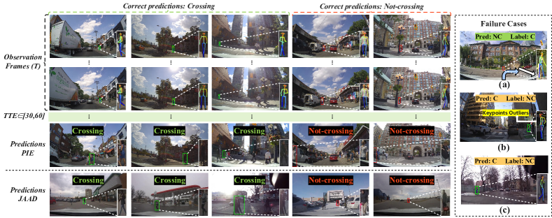
Fig. 5 presents visualized predictions for the PIE and JAAD datasets, with the first two rows showing the observation period before TTE and the last rows depicting the action period. Additionally, failure cases are shown, typically falling into three categories: vertical crossing when the ego-vehicle is turning, keypoint outliers, and pedestrians waiting by the roadside. These areas can be addressed in future work.
V Conclusion
In this study, we propose GTransPDM, a Graph-embedded Transformer with a Position Decoupling Module for pedestrian crossing intention prediction. It effectively fuses multi-modal features with position, ego-vehicle motion, and pedestrian pose, ensuring a lightweight, real-time application. The Position Decoupling Module captures positional variations with road-boundary-like reference lines and bounding box changes to decompose lateral movements and simulate depth in on-board image views. Additionally, a GCN-based Transformer models the spatial and temporal dynamics of pedestrian skeletons. Our method predicts pedestrian crossing behavior 1-2 seconds in advance, achieving 92% accuracy on the PIE dataset and 87% on the JAAD dataset, with a run time of 0.05ms, surpassing existing state-of-the-art solutions. For simplicity and efficiency, this work models road boundaries as constant using reference lines. Future work could improve this by incorporating semantic segmentation for dynamic road border representations.
ACKNOWLEDGMENT
This work was partly supported by the Scientific and Technological Developing Project of Jilin Province (20240402076GH); and the China Scholarship Council (202306170152). Antonio M. López acknowledges the financial support to his general research activities given by ICREA under the ICREA Academia Program. Antonio also thanks the Spanish grant PID2020-115734RB-C21 (MCIN/AEI/10.13039/501100011033) for the synergies generated for this paper. Antonio and Chen acknowledge the support of the Generalitat de Catalunya CERCA Program and its ACCIO agency to CVC’s general activities.
References
- [1] K. Saleh, M. Hossny, and S. Nahavandi, “Real-time intent prediction of pedestrians for autonomous ground vehicles via spatio-temporal densenet,” in Proc. Int. Conf. Robot. Autom. (ICRA), 2019, pp. 9704–9710.
- [2] C. Lin, S. Zhang, B. Gong, and H. Liu, “Near-crash risk identification and evaluation for takeout delivery motorcycles using roadside lidar,” Accid. Anal. Prev., vol. 199, p. 107520, 2024.
- [3] I. Kotseruba, A. Rasouli, and J. K. Tsotsos, “Benchmark for evaluating pedestrian action prediction,” in Proc. IEEE/CVF Winter Conf. Appl. Comput. Vis. (WACV), 2021, pp. 1258–1268.
- [4] D. Yang, H. Zhang, E. Yurtsever, K. A. Redmill, and Ü. Özgüner, “Predicting pedestrian crossing intention with feature fusion and spatio-temporal attention,” IEEE Trans. Intell. Veh., vol. 7, no. 2, pp. 221–230, Mar. 2022.
- [5] B. Yang, J. Zhu, C. Hu, Z. Yu, H. Hu, and R. Ni, “Faster pedestrian crossing intention prediction based on efficient fusion of diverse intention influencing factors,” IEEE Trans. Transport. Electr., pp. 1–1, Feb. 2024.
- [6] Z. Zhang, R. Tian, and Z. Ding, “Trep: Transformer-based evidential prediction for pedestrian intention with uncertainty,” in Proc. AAAI Conf. Artif. Intell. (AAAI), vol. 37, no. 3, 2023, pp. 3534–3542.
- [7] S. Ahmed, A. Al Bazi, C. Saha, S. Rajbhandari, and M. N. Huda, “Multi-scale pedestrian intent prediction using 3d joint information as spatio-temporal representation,” Expert Syst. Appl., vol. 225, p. 120077, 2023.
- [8] Z. Fang and A. M. López, “Intention recognition of pedestrians and cyclists by 2d pose estimation,” IEEE Trans. Intell. Transport. Syst., vol. 21, no. 11, pp. 4773–4783, 2020.
- [9] Y. Ling, Z. Ma, Q. Zhang, B. Xie, and X. Weng, “Pedast-gcn: Fast pedestrian crossing intention prediction using spatial–temporal attention graph convolution networks,” IEEE Trans. Intell. Transport. Syst., pp. 1–14, 2024.
- [10] J. Lorenzo, I. Parra, and M. Sotelo, “Intformer: Predicting pedestrian intention with the aid of the transformer architecture,” arXiv preprint arXiv:2105.08647, 2021.
- [11] A. Rasouli and I. Kotseruba, “Pedformer: Pedestrian behavior prediction via cross-modal attention modulation and gated multitask learning,” in Proc. IEEE Int. Conf. Robot. Autom. (ICRA), 2023, pp. 9844–9851.
- [12] B. Yang, W. Zhan, P. Wang, C. Chan, Y. Cai, and N. Wang, “Crossing or not? context-based recognition of pedestrian crossing intention in the urban environment,” IEEE Trans. Intell. Transport. Syst., vol. 23, no. 6, pp. 5338–5349, 2022.
- [13] A. Rasouli, I. Kotseruba, and J. K. Tsotsos, “Pedestrian action anticipation using contextual feature fusion in stacked rnns,” arXiv preprint arXiv:2005.06582, 2020.
- [14] K. Kitchat, Y.-L. Chiu, Y.-C. Lin, M.-T. Sun, T. Wada, K. Sakai, W.-S. Ku, S.-C. Wu, A. A.-K. Jeng, and C.-H. Liu, “Pedcross: Pedestrian crossing prediction for auto-driving bus,” IEEE Trans. Intell. Transport. Syst., vol. 25, no. 8, pp. 8730–8740, 2024.
- [15] K. D. Katyal, G. D. Hager, and C.-M. Huang, “Intent-aware pedestrian prediction for adaptive crowd navigation,” in Proc. Int. Conf. Robot. Autom. (ICRA), 2020, pp. 3277–3283.
- [16] L. Achaji, J. Moreau, T. Fouqueray, F. Aioun, and F. Charpillet, “Is attention to bounding boxes all you need for pedestrian action prediction?” in Proc. IEEE Intell. Veh. Symp. (IV), 2022, pp. 895–902.
- [17] I. Kotseruba, A. Rasouli, and J. K. Tsotsos, “Do they want to cross? understanding pedestrian intention for behavior prediction,” in Proc. IEEE Intell. Veh. Symp. (IV), 2020, pp. 1688–1693.
- [18] M. Dang, Y. Jin, P. Hang, L. Crosato, Y. Sun, and C. Wei, “Coupling intention and actions of vehicle–pedestrian interaction: A virtual reality experiment study,” Accid. Anal. Prev., vol. 203, p. 107639, 2024.
- [19] F. Soares, E. Silva, F. Pereira, C. Silva, E. Sousa, and E. Freitas, “To cross or not to cross: Impact of visual and auditory cues on pedestrians’ crossing decision-making,” Transp. Res. Part F Traffic Psychol. Behav., vol. 82, pp. 202–220, 2021.
- [20] Z. Zhou, Z. Wang, Y. Liu, Z. Chen, and Y. Xu, “Dependent hidden markov model for pedestrian intention prediction: considering multivariate interaction force,” Transp. A Transp. Sci., pp. 1–24, 2024.
- [21] T. Fu, X. Yu, B. Xiong, C. Jiang, J. Wang, Q. Shangguan, and W. Xu, “A method in modeling interactive pedestrian crossing and driver yielding decisions during their interactions at intersections,” Transp. Res. Part F Traffic Psychol. Behav., vol. 88, pp. 37–53, 2022.
- [22] Y. Zhang, K. Guo, W. Guo, J. Zhang, and Y. Li, “Pedestrian crossing detection based on hog and svm,” J. Cybersecurity, vol. 3, no. 2, p. 79, 2021.
- [23] A. Dosovitskiy, “An image is worth 16x16 words: Transformers for image recognition at scale,” arXiv preprint arXiv:2010.11929, 2020.
- [24] Y. Zhou, G. Tan, R. Zhong, Y. Li, and C. Gou, “Pit: Progressive interaction transformer for pedestrian crossing intention prediction,” IEEE Trans. Intell. Transport. Syst., vol. 24, no. 12, pp. 14 213–14 225, 2023.
- [25] F. Scarselli, M. Gori, A. C. Tsoi, M. Hagenbuchner, and G. Monfardini, “The graph neural network model,” IEEE Trans. Neural Netw., vol. 20, no. 1, pp. 61–80, 2009.
- [26] M. I. Perdana, W. Anggraeni, H. A. Sidharta, E. M. Yuniarno, and M. H. Purnomo, “Early warning pedestrian crossing intention from its head gesture using head pose estimation,” in 2021 Proc. Int. Sem. Intell. Technol. Its Appl. (ISITIA). IEEE, 2021, pp. 402–407.
- [27] S. Yan, Y. Xiong, and D. Lin, “Spatial temporal graph convolutional networks for skeleton-based action recognition,” in Proc. AAAI Conf. Artif. Intell. (AAAI), vol. 32, no. 1, 2018.
- [28] P. Velickovic, G. Cucurull, A. Casanova, A. Romero, P. Lio, Y. Bengio, et al., “Graph attention networks,” stat, vol. 1050, no. 20, pp. 10–48 550, 2017.
- [29] M. N. Riaz, M. Wielgosz, A. G. Romera, and A. M. López, “Synthetic data generation framework, dataset, and efficient deep model for pedestrian intention prediction,” in 2023 IEEE Int. Conf. Intell. Transp. Syst. (ITSC). IEEE, 2023, pp. 2742–2749.
- [30] X. Zhang, P. Angeloudis, and Y. Demiris, “St crossingpose: A spatial-temporal graph convolutional network for skeleton-based pedestrian crossing intention prediction,” IEEE Trans. Intell. Transport. Syst., vol. 23, no. 11, pp. 20 773–20 782, 2022.
- [31] A. Vaswani, “Attention is all you need,” Adv. Neural Inf. Process. Syst. (NeurIPS), 2017.
- [32] H.-G. Chi, M. H. Ha, S. Chi, S. W. Lee, Q. Huang, and K. Ramani, “Infogcn: Representation learning for human skeleton-based action recognition,” in Proc. IEEE/CVF Conf. Comput. Vis. Pattern Recognit. (CVPR), 2022, pp. 20 154–20 164.
- [33] Y. Liu, H. Zhang, D. Xu, and K. He, “Graph transformer network with temporal kernel attention for skeleton-based action recognition,” Knowl.-Based Syst., vol. 240, p. 108146, 2022.
- [34] H. Wang, A. Wang, F. Su, and D. C. Schwebel, “The effect of age and sensation seeking on pedestrian crossing safety in a virtual reality street,” Transp. Res. Part F Traffic Psychol. Behav., vol. 88, pp. 99–110, 2022.
- [35] M. Azarmi, M. Rezaei, H. Wang, and S. Glaser, “Pip-net: Pedestrian intention prediction in the wild,” arXiv preprint arXiv:2402.12810, 2024.
- [36] M. Upreti, J. Ramesh, C. Kumar, B. Chakraborty, V. Balisavira, M. Roth, V. Kaiser, and P. Czech, “Traffic light and uncertainty aware pedestrian crossing intention prediction for automated vehicles,” in Proc. IEEE Intell. Veh. Symp. (IV), 2023, pp. 1–8.
- [37] B. Liu, E. Adeli, Z. Cao, K.-H. Lee, A. Shenoi, A. Gaidon, and J. C. Niebles, “Spatiotemporal relationship reasoning for pedestrian intent prediction,” IEEE Robot. Autom. Lett., vol. 5, no. 2, pp. 3485–3492, 2020.
- [38] S. Zhao, H. Li, Q. Ke, L. Liu, and R. Zhang, “Action-vit: Pedestrian intent prediction in traffic scenes,” IEEE Signal Process. Lett., vol. 29, pp. 324–328, 2021.
- [39] T. N. Kipf and M. Welling, “Semi-supervised classification with graph convolutional networks,” arXiv preprint arXiv:1609.02907, 2016.
- [40] A. Rasouli, I. Kotseruba, and J. K. Tsotsos, “Are they going to cross? a benchmark dataset and baseline for pedestrian crosswalk behavior,” in Proc. IEEE Int. Conf. Comput. Vis. Workshops (ICCVW), 2017, pp. 206–213.
- [41] A. Rasouli, I. Kotseruba, T. Kunic, and J. K. Tsotsos, “Pie: A large-scale dataset and models for pedestrian intention estimation and trajectory prediction,” in Proc. IEEE/CVF Int. Conf. Comput. Vis. (ICCV), 2019, pp. 6262–6271.
- [42] H.-S. Fang, J. Li, H. Tang, C. Xu, H. Zhu, Y. Xiu, Y.-L. Li, and C. Lu, “Alphapose: Whole-body regional multi-person pose estimation and tracking in real-time,” IEEE Trans. Pattern Anal. Machine Intell., vol. 45, no. 6, pp. 7157–7173, 2022.
- [43] D. R. Cox, “The regression analysis of binary sequences,” J. R. Stat. Soc. Ser. B Stat. Methodol., vol. 20, no. 2, pp. 215–232, 1958.
- [44] A. Rasouli, M. Rohani, and J. Luo, “Bifold and semantic reasoning for pedestrian behavior prediction,” in Proc. IEEE/CVF Int. Conf. Comput. Vis. (ICCV)., 2021, pp. 15 580–15 590.
- [45] P. R. G. Cadena, Y. Qian, C. Wang, and M. Yang, “Pedestrian graph +: A fast pedestrian crossing prediction model based on graph convolutional networks,” IEEE Trans. Intell. Transport. Syst., vol. 23, no. 11, pp. 21 050–21 061, 2022.
- [46] A. Bhattacharyya, M. Fritz, and B. Schiele, “Long-term on-board prediction of people in traffic scenes under uncertainty,” in Proc. IEEE/CVF Conf. Comput. Vis. Pattern Recognit. (CVPR), 2018, pp. 4194–4202.
- [47] J. Gesnouin, S. Pechberti, B. Stanciulcscu, and F. Moutarde, “Trouspi-net: Spatio-temporal attention on parallel atrous convolutions and u-grus for skeletal pedestrian crossing prediction,” in 2021 IEEE Int. Conf. Autom. Face Gesture Recognit. (FG 2021). IEEE, 2021, pp. 01–07.
- [48] L. Yang, B. Kang, Z. Huang, X. Xu, J. Feng, and H. Zhao, “Depth anything: Unleashing the power of large-scale unlabeled data,” in Proc. IEEE/CVF Conf. Comput. Vis. Pattern Recognit. (CVPR), 2024, pp. 10 371–10 381.