SetPINNs: Set-based Physics-informed
Neural Networks

Abstract

Physics-Informed Neural Networks (PINNs) have emerged as a promising method for approximating solutions to partial differential equations (PDEs) using deep learning. However, PINNs, based on multilayer perceptrons (MLP), often employ point-wise predictions, overlooking the implicit dependencies within the physical system such as temporal or spatial dependencies. These dependencies can be captured using more complex network architectures, for example CNNs or Transformers. However, these architectures conventionally do not allow for incorporating physical constraints, as advancements in integrating such constraints within these frameworks are still lacking. Relying on point-wise predictions often results in trivial solutions. To address this limitation, we propose SetPINNs, a novel approach inspired by Finite Elements Methods from the field of Numerical Analysis. SetPINNs allow for incorporating the dependencies inherent in the physical system while at the same time allowing for incorporating the physical constraints. They accurately approximate PDE solutions of a region, thereby modeling the inherent dependencies between multiple neighboring points in that region. Our experiments show that SetPINNs demonstrate superior generalization performance and accuracy across diverse physical systems, showing that they mitigate failure modes and converge faster in comparison to existing approaches. Furthermore, we demonstrate the utility of SetPINNs on two real-world physical systems.

1 Introduction

Mesh-based numerical methods such as Finite Elements and Finite Volumes have long been preferred solvers for complex physical simulation problems involving partial differential equations (PDEs). However, solving high-dimensional PDEs with these methods can be computationally intractable [13]. In response, mesh-free methods based on machine learning—notably physics-informed neural networks (PINNs)—have emerged as efficient alternatives [29].

PINNs have been successfully deployed across a wide range of systems, including fluid mechanics [5] and climate forecasting [36]. However, PINNs can struggle when the PDE’s solution contains high-frequency or multi-scale features. In such cases, known as “failure modes” [26, 9, 19, 12, 40, 46, 22], optimization can become trapped in local minima, resulting in overly smooth approximations diverging from the ground-truth solutions. Figure 1 demonstrates this issue through a 1D reaction equation, where state-of-the-art PINNs fail to approximate the true solution, instead producing overly smooth, trivial solutions. We discuss mitigating such and other failure modes in detail in Section 5.

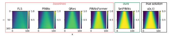
Figure 1: Failure Modes of PINNs applied to a 1D reaction equation. Conventional PINNs often result in overly smooth, trivial solutions. In contrast, the proposed SetPINNs show consistent performance that more closely aligns with the true solution $u(x,t)$. The figure reports mean predictions averaged over ten runs.

In various mathematical and computational methods, temporal and spatial dependencies are implicitly taken into account. For instance in Finite Element Methods (FEM), such dependencies are addressed through the discretization of the domain into smaller elements [48]. Here each element consists of multiple nodes (points), each of which is connected to neighboring elements through shared nodes, and the solution is computed over these elements. Each element has its own set of basis functions defined locally within the element’s domain. The main idea is that the solution at one point in space can influence the solution at neighboring points. This interaction is captured through the basis functions, ensuring that the model reflects the physical reality of the system under study. In contrast, PINNs ignore these crucial dependencies, instead employing point-wise predictions [46].

Analogous to FEM [10, 48], which uses a set of basis functions to process an element, we model temporal and spatial dependencies by representing an element as a set and processing it using neural networks. As points within an element in the domain are invariant to any ordering, representing them as sets is a natural choice. Set-based learning addresses problems where a set is mapped to a target label or to a set of labels where each label corresponds to one element of the input set. Deep learning provides an efficient mechanism for learning dependencies or affinities within a set [43, 21].

The proposed set-based PINNs aim to integrate advantages of traditional FEM into PINNs. Set-based PINNs take dependencies between neighboring points into account, as in FEM, while being completely data-driven, mesh-free, and respecting the physical constraints as in PINNs. SetPINNs capture dependencies by grouping inputs into sets of nearby points. We use the attention mechanism to efficiently capture the dependencies since the computation of additive attention is invariant to permutations of its input. This allows to model dependencies within sets of input elements. To correctly apply the physical constraints, we introduce a set-wise physics loss in place of the traditional point-wise PINN loss. Our experiments show the effectiveness of SetPINNs for solving PDEs, but also their practical relevance as grey-box models in two application domains where limited experimental data may be available: predicting activity coefficients for molecules and predicting agglomerate breakage. SetPINNs are theoretically grounded, easy to implement, and not restricted in terms of the physical domain where they are applicable. SetPINNs can be employed on data from any domain, such as temporal, spatial, or elemental.

Contributions. The key contributions can be summarized as follows:

• Novel approach. We propose SetPINNs, a novel set-to-set PINN approach inspired by Finite Element Methods that represents neighboring points in a physical domain using sets and efficiently learns them using a set-wise physics loss.

• Avoids trivial solutions. Our experiments show that SetPINNs outperform existing state-of-the-art PINN architectures in a wide range of scenarios and avoid trivial solutions.

• Extensive experiments. With our experiments on four physical domains and two real-world physical systems, we demonstrate that SetPINNs are more robust than existing PINN approaches. They also outperform a state-of-the-art physical model for predicting activity coefficients.

We begin by describing related work in Section 2. Then, we present our problem statement, theoretical foundations of PINNs and FEM, and main method in Section 3. We demonstrate the effectiveness of our work with experiments in Section 4. Finally, we discuss the results and conclude our work in Sections 5 and 6, respectively.

2 Related work

Physics-informed neural networks.

Methods to solve PDEs using neural networks by constraining the loss function using the underlying PDE structure have existed for a long time [20, 27]. With recent advancements in deep learning, the idea of using neural networks as PDE solvers has seen a renaissance in the form of physics-informed neural networks (PINNs) [29].

PINNs add a residual term to the loss function, penalizing predictions that do not satisfy the underlying PDE. This approach has spawned a lot of follow-up work, e.g., extending PINNs for uncertainty quantification [14], analyzing convergence behavior [34], and understanding and mitigating failure modes [40]. PINNs have been successfully applied to a variety of problems including simulating blood flow in cardiovascular structures [30], climate forecasting[36], and fluid mechanics [5], among many others. However, in practice MLP-based PINN architectures often fail to achieve stable training and produce accurate predictions.

Wang et al. [39] attributed this pathological behavior to multi-scale interactions between different terms in the PINNs loss function, ultimately leading to stiffness in the gradient flow dynamics, which, consequently, introduces stringent stability requirements on the learning rate. Other work has indicated certain inherent failure modes, particularly when confronted with PDEs having high-frequency or multiscale features [28, 12, 19, 40, 46, 22]. In these cases, the predictions collapse to overly smooth trivial solutions.

This challenge has prompted investigations from four different perspectives: 1. employing different training schemes, 2. using data interpolation techniques, 3. designing new model architectures, or 4. incorporating dependencies present in the domain [46]. Different training schemes [25, 19, 38, 40] can incur high computational costs. For example, Seq2Seq by Krishnapriyan et al. [19] requires training multiple neural networks sequentially, while other approaches face convergence issues due to error accumulation. Data interpolation strategies [15, 23, 38, 40] employ regularization based on simulations or real-world scenarios [47, 8], but acquiring ground truth data remains challenging. In terms of alternative architectures, Bu and Karpatne [4] proposed QRes (Quadratic Residual Networks), which introduce quadratic non-linearity before applying activation functions at every layer. Similarly, Wong et al. [41] highlighted the benefits of learning in sinusoidal spaces with PINNs using the First-Layer Sine (FLS) method. Another approach by Wang et al. [40] integrates the Neural Tangent Kernel (NTK) with PINNs, constructing kernels $K\in\mathbb{R}^{D\times P}$, where $D$ is the sample size and $P$ is the number of model parameters. This method, however, faces scalability issues as sample size or model parameters increase. Recently, Zhao et al. [46] introduced PINNsFormer, which accounts for implicit temporal dependencies in the domain and outperforms existing methods. However, PINNsFormer is limited to the temporal domain and does not generalize well to other diverse physical domains.

Existing PINN approaches do not account for the crucial implicit dependencies inherent in the physical domain. In contrast, SetPINNs, inspired by Finite Element Methods, model these dependencies.

Deep learning for sets.

Elements in a set do not follow any order. Set-based learning problems include tasks where a set is mapped to a target label or a set of labels. Recently, deep learning has become popular in addressing set-based learning problems with the introduction of Deep Sets [43, 37], which provide an efficient mechanism for learning dependencies or affinities within a set. Extending this, Lee et al. [21] introduce Set-Transformers, showing that the attention mechanism, the backbone of the Transformer architecture [35], is an excellent choice for tackling set-based learning problems as it is invariant to input permutation.

Many domains have inputs best represented as sets. Examples include a point cloud obtained from a LIDAR sensor [42], a group of atoms forming a molecule [44], graph structures [33, 37], or a collection of objects appearing in an image [43]. This has led to many interesting applications, such as point cloud classification [43], image tagging [43], partitioning for particle physics [33], designing high-entropy alloys [45], and gait recognition [6], among others.

With SetPINNs, we propose to represent neighboring points in a physical domain as sets and learn dependencies between them using a Transformer network. Thereby, we are to the best of our knowledge the first to combine set-based and physics-informed learning, leading to a novel set-wise physics loss that enforces a soft physical constraint at the set level.

3 Methodology

We begin with preliminaries in Section 3.1 and present our proposed method in Section 3.2. Note that, for simplicity, we present our method by exemplifying the spatio-temporal domain. In general, as shown in our experiments, the proposed method is versatile and can be easily extended to other domains as well.

3.1 Preliminaries

In this section, we will start with the problem statement, then introduce PINNs, and finally explain the necessary background in finite-element methods.

3.1.1 Problem statement

We consider the problem of incorporating physical laws into neural network training to solve PDEs, while accounting for the interdependencies present in the domain. Conventional PINN approaches use point-wise predictions to estimate the solution $u(t,x)$. However, this approach overlooks the implicit relationships between different points in the area surrounding $(t,x)$.

3.1.2 Physics-informed Neural Networks (PINNs)

Let us consider nonlinear partial differential equations (PDEs) of the general form:

$$u_{t}+\mathcal{N}[u]=0,\quad x\in\Omega,t\in[0,T],$$ (1)

where $u(t,x)$ is the latent solution of the PDE, $u_{t}$ is the partial derivative of $u$ w.r.t. $t$, $\mathcal{N}[\cdot]$ is a nonlinear differential operator, $\Omega\in\mathbb{R}^{d}$ is an open, bounded, connected spatial domain, and $[0,T]$ is the time interval.

In the PINNs approach introduced by Raissi et al. [29], a physics-informed neural network $f:=u_{t}+\mathcal{N}[u]$ is defined, where $u(t,x)$ is approximated by a fully connected neural network with parameters $\theta$. $u(t,x)$ and $f(t,x)$ share the same parameters $\theta$, and the inputs $(t,x)$ are randomly sampled from the domain. They employ automatic differentiation, thus avoiding the need for discretizing the (space-time) domain and relying instead on random sampling. The weights of the neural networks are optimized during training with the following loss function:

$$\mathcal{L}_{\textmd{PINNs}} =\frac{1}{N_{f}}\sum_{i=1}^{N_{f}}\left\lVert f(t_{f}^{i},x_{f}^{i})\right\rVert^{2}+\frac{1}{N_{u}}\sum_{i=1}^{N_{u}}\left\lVert u(t_{u}^{i},x_{u}^{i})-u^{i}\right\rVert^{2},$$ (2)

where $\{t_{u}^{i},x_{u}^{i},u^{i}\}_{i=1}^{N_{u}}$ denotes the initial and boundary data on $u(t,x)$, and $\{t_{f}^{i},x_{f}^{i}\}_{i=1}^{N_{f}}$ denotes the collocation points for the residual $f(t,x)$. $N_{u}$ and $N_{f}$ denote the number of initial and boundary points, and collocation points, respectively. The differential operator $\mathcal{N}$ and other derivatives are evaluated using automatic differentiation.

3.1.3 Finite-element methods

In this section, we lay out the theoretical foundations of our method. First, we present the background on Finite Element Methods (FEM) [48], which form the basis of our main idea. Then, we establish implicit dependencies between neighboring points in a domain.

For the PDE defined in Eq. 1, the FEM involves discretizing $\Omega$ into a finite number $N$ of elements (e.g., triangles or tetrahedra) and representing $u$ as a linear combination of basis functions (typically piecewise polynomials) defined on these elements. Formally, let $\{\phi_{i}(x)\}_{i=1}^{N}$ be the basis functions associated with the spatial discretization, and approximate $u$ as $u_{h}(x,t)=\sum_{i}U_{i}(t)\phi_{i}(x)$, where $U_{i}(t)$ are the time-dependent coefficients. The PDE is then transformed into a system of ordinary differential equations (ODEs) by applying a weighted residual approach, typically the Galerkin method, which ensures that the residuals are orthogonal to the space spanned by the basis functions. This results in a system of ODEs for the coefficients $U_{i}(t)$, which can be solved using appropriate integration schemes.

The FEM process results in a system of coupled equations where the solution at any point depends on the solutions at neighboring points due to the overlapping support of the basis functions. Consequently, the FEM inherently introduces implicit dependencies between the approximations at neighboring points, ensuring a coherent and smooth numerical solution across the entire domain.

Theorem 3.1.1

Let $u(x,t)$ be the solution to the partial differential equation $u_{t}+\mathcal{N}[u]=0$ over $x\in\Omega$ and $t\in[0,T]$. The approximate solution $u_{h}(x,t)$ computed using the finite element method (FEM) at two neighboring points $(x_{1},t_{1})$ and $(x_{2},t_{2})$ is dependent on each other; i.e., the solutions $u_{h}(x_{1},t_{1})$ and $u_{h}(x_{2},t_{2})$ are implicitly coupled through their shared finite element basis functions and the discretization scheme.

The proof is provided in Appendix A. The theorem is empirically validated in Appendix B.7.

We now aim to extend this result from FEM to physics-informed deep learning. We propose to model implicit dependencies between two neighboring points in a domain using sets and move from point-wise predictions in conventional PINN approaches to set-wise predictions.

3.2 SetPINNs

We introduce a novel method featuring a set-based PINN architecture, namely SetPINNs, thereby (1) exploiting the implicit dependencies within elements by learning affinities between neighboring points and (2) accurately approximating solutions of multiple points in the domain at once.

We illustrate our main idea in Figure 2, where first we exemplify the set generation process for several data domains, and then each set is processed through a Mixer Network, Set Processor, and finally a PDE Probe to predict the solution for each element in the set. The parameters of SetPINNs are learned using a set-wise physics loss.

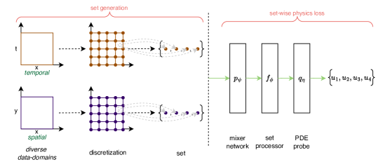
Figure 2: Overview of our method. On the left, we exemplify the set generation process for diverse data domains. Sets are formed from nearby points in a grid. Each set is then processed through a Mixer Network, Set Processor, and finally a PDE Probe to predict the solution for each element in the set. The parameters of SetPINNs are learned using a set-wise physics loss.

Our method consists of four main components: Set Generator, Mixer Network, Set Processor, and a PDE Probe, which we will explain in turn. Then, we present the learning scheme.

3.2.1 Model

Set Generator.

Analogous to FEM, as discussed in Sec 3.1.3, we first discretize the domain $\Omega$ into $N$ elements $\{\Omega_{e}\}_{e=1}^{N}$. We then sample $K_{e}$ points from each element $\Omega_{e}$ and represent them as a set $\mathcal{S}_{e}$. Considering a spatio-temporal domain, the set generator can be defined as:

$$\Omega_{e}\xRightarrow{\textmd{set-generator}}\mathcal{S}_{e}:\{(x^{0}_{e},t^{0}_{e}),(x^{1}_{e},t^{1}_{e}),\dots,(x^{K_{e}}_{e},t^{K_{e}}_{e})\},$$ (3)

where $(x^{i}_{e},t^{i}_{e})$ is a point in $\Omega_{e}$, and the generator outputs a set $\mathcal{S}_{e}$ with $K_{e}$ elements.

Mixer Network.

A point $(x^{i}_{e},t^{i}_{e})$ in the domain typically contains low-dimensional information regarding its state. Since SetPINNs focus on modeling interactions between multiple points in the set, directly feeding low-dimensional data is insufficient for accurately learning the affinities between the points. To address this, we propose using a Mixer Network in conjunction with the Set Processor. The Mixer Network learns a parameterized function $p_{\psi}$ that mixes state variables and transforms low-dimensional state representations into high-dimensional vectors, akin to word embeddings in NLP. These vectors represent the state within a high-dimensional space. For our use cases, we opt for a simple fully-connected layer for the Mixer Network, but it can also be a more sophisticated architecture depending on the problem.

$$\mathcal{M}_{e}=p_{\psi}(\mathcal{S}_{e})\quad s.t.\quad\mathcal{M}_{e}:\{\mathcal{M}_{e}^{0},\mathcal{M}_{e}^{1},\dots,\mathcal{M}_{e}^{K_{e}}\},$$ (4)

where $\mathcal{M}_{e}^{i}$ represents the embedding of point $(x^{i}_{e},t^{i}_{e})$ in the set $\mathcal{S}_{e}$. $\psi$ are the learnable parameters of the Mixer Network. Notably the Mixer Network transforms $\mathcal{S}_{e}\in\mathbb{R}^{K_{e}\times r}$ to $\mathcal{M}_{e}\in\mathbb{R}^{K_{e}\times d}$ where $d\gg r$.

Set Processor.

For each element $\Omega_{e}$, we seek an approximate solution $u_{e}$ that satisfies the PDE in the domain $\Omega$. Using the Set Generator and Mixer Network, we have transformed $\Omega_{e}$ into $\mathcal{M}_{e}$, which is a set of high-dimensional vectors representing each point in $\Omega_{e}$. Notably, finding $u_{e}$ is now a set-learning task. We seek to learn a solution $u_{e}^{i}$ for each element $\mathcal{M}_{e}^{i}$ of the set $\mathcal{M}_{e}$. To achieve this, the Set Processor must meet two criteria: (R1) It must operate as a set-to-set network, and (R2) It must maintain permutational equivariance. Thus, in our experiments, we use the Transformer network to process $\mathcal{M}_{e}$. Transformers are originally used in NLP tasks, but the attention mechanism, which is the backbone of Transformers, is equivariant to the input permutations. When used on sets, Transformers can capture affinities among elements in the input set. This satisfies the requirements for using them to model the set $\mathcal{M}_{e}$.

$$\mathcal{O}_{e}=f_{\phi}(\mathcal{M}_{e})\quad s.t.\quad\mathcal{O}_{e}:\{\mathcal{O}_{e}^{0},\mathcal{O}_{e}^{1},\dots,\mathcal{O}_{e}^{K_{e}}\},$$ (5)

where $\mathcal{O}_{e}^{i}$ represents the transformed representation of each element $\mathcal{M}_{e}^{i}$ in set $\mathcal{M}_{e}$. $\phi$ are the learnable parameters of Set Processor. Notably the Set Processor transforms $\mathcal{M}_{e}\in\mathbb{R}^{K_{e}\times d}$ to $\mathcal{O}_{e}\in\mathbb{R}^{K_{e}\times d}$.

PDE Probe.

After processing $\mathcal{M}_{e}$ using the Set Processor we get a transformed representation $\mathcal{O}_{e}$ where each element now has interacted and has information regarding other elements in the set $\Omega_{e}$. We now predict solution $u_{e}$ using a PDE Probe.

$$u_{e}=q_{\eta}(\mathcal{O}_{e})\quad s.t.\quad u_{e}:\{u_{e}^{0},u_{e}^{1},\dots,u_{e}^{K_{e}}\},$$ (6)

where $u_{e}^{i}$ represents the solution of each element $\mathcal{O}_{e}^{i}$ in set $\mathcal{O}_{e}$. $\eta$ are the learnable parameters of PDE Probe. Notably the PDE Probe transforms $\mathcal{O}_{e}\in\mathbb{R}^{K_{e}\times d}$ to $u_{e}\in\mathbb{R}^{K_{e}\times 1}$.

3.2.2 Learning scheme

Conventional PINN approaches focus on point-wise prediction and are trained using a point-wise PINN loss, as shown in Eq. 2. Since the proposed set-based approach employs set-wise predictions, we adapt the existing PINN loss to handle sets. In SetPINNs, each generated set $\Omega_{e}$ is associated with a predicted solution $u_{e}$. This enables us to compute the $n$-th order gradient with respect to the state variables $x$ and $t$. For instance, for any given set $\Omega_{e}$ and its corresponding solution $u_{e}$, the first-order gradient can be expressed as $\frac{\partial u_{e}}{\partial x_{e}}=\left\{\frac{\partial u_{e}^{i}}{\partial x_{e}^{i}}\right\}_{i=0}^{K_{e}}$ and $\frac{\partial u_{e}}{\partial t_{e}}=\left\{\frac{\partial u_{e}^{i}}{\partial t_{e}^{i}}\right\}_{i=0}^{K_{e}}$, respectively.

This scheme of computing gradients of predicted sets with respect to input sets can be easily extended to higher-order derivatives and is applicable to sets of residual, boundary, and initial points.

By these considerations, we now adapt the point-wise PINN objective to the set-wise SetPINNs objective:

$$\mathcal{L}_{\textmd{SetPINNs}} =\frac{\lambda_{f}}{N_{f}}\sum_{e=1}^{|N|}\sum_{i=1}^{K_{e}}\left\lVert f_{\theta}(t_{e}^{i},x_{e}^{i})\right\rVert^{2}+\frac{\lambda_{u}}{N_{u}}\sum_{e=1}^{|M|}\sum_{i=1}^{K_{e}}\left\lVert u_{\theta}(t_{e}^{i},x_{e}^{i})-u^{i}_{e}\right\rVert^{2},$$ (7)

where $N$ and $M$ are the sets generated from the residual, boundary and initial data points, respectively, and $K_{e}$ is the number of elements in a set $e$. $\lambda_{f}$ and $\lambda_{u}$ are weighting parameters, and $\theta:=\{\psi,\phi,\eta\}$. $N_{f}$ and $N_{u}$ comprise all the points in $N$ and $M$, respectively.

4 Experiments

In this section, we empirically show that SetPINNs are robust and accurate across diverse physical systems. We first briefly discuss and describe comparison models in Section 4.1. Then, we benchmark all the models on diverse physical systems in Section 4.2. We also show the utility of SetPINNs for two real-world physical systems in Section 4.3.

4.1 Model setup

For baseline models, we select the standard MLP-based PINNs [29], First-Layer Sine (FLS) [41], Quadratic Residual Networks (QRes) [4], and PINNsFormer [46]. These are standard and current state-of-the-art models [46]. For fairness, we ensure that all baselines maintain approximately the same number of parameters. SetPINNs follows a simple encoder-decoder Transformer architecture based on PINNsFormer [46]. For the training routine, as a standard practice, we train our models using the Adam optimizer [18] followed by L-BFGS [32]. We evaluate our models using the standard relative Mean Absolute Error (rMAE) and relative Root Mean Squared Error (rRMSE). SetPINNs are trained using the objective in Eq. 7 with $\lambda_{f}=\lambda_{u}=1$. More details on model architectures and hyperparameter selection are provided in Appendix B.2. Ablation studies for the hyperparameters can be found in Appendix B.7.

4.2 Benchmarking PDE solvers

Model	1D-Reaction	Convection	1D-Wave	Navier-Stokes
PINNs	$0.385\pm 0.09$	$0.536\pm 0.14$	$0.731\pm 0.13$	$5.703\pm 2.46$
QRES	$0.271\pm 0.12$	$0.245\pm 0.06$	$0.672\pm 0.14$	$2.235\pm 1.34$
FLS	$0.502\pm 0.06$	$0.332\pm 0.08$	$0.650\pm 0.11$	$3.016\pm 0.91$
PINNsFormer	$0.133\pm 0.05$	$0.102\pm 0.04$	$0.531\pm 0.12$	$0.841\pm 0.29$
SetPINNs (ours)	$\mathbf{0.046\pm 0.00}$	$\mathbf{0.031\pm 0.01}$	$\mathbf{0.332\pm 0.04}$	$\mathbf{0.218\pm 0.08}$

Table 1: SetPINNs as a robust and accurate PDE solver. rRMSE scores of existing state-of-the-art models and SetPINNs on diverse physical systems show that SetPINNs significantly outperform existing baselines with low error and provide robust predictions, as showcased by the least variance. Significant results (p-value < 0.05) are highlighted in bold, and the variance is captured over ten runs.

For benchmarking, we rely on four types of PDEs from diverse systems: 1D-reaction, 1D-wave, Convection, and Navier-Stokes that follow established setups for fair comparisons [29, 19, 39, 46]. For training, we uniformly sample initial and boundary points $N_{u}=50$ and construct a uniform $50\times 50$ mesh for residual points $N_{f}$. Similarly, for the validation and test sets, we deal with $21$ and $101$ uniformly sampled points respectively. For PINNs, QRES, and FLS, we perform point-wise predictions with each point as an independent input. For PINNsFormer, we create a pseudo sequence for input as described by the authors [46]. For SetPINNs, we sample four points from the domain in close proximity to create set inputs for both initial and boundary, as well as for residual points, respectively.

To evaluate the performance of selected models, we run them using ten different seeds to capture the variance and perform a two-tailed t-test to establish significance. The relative Root Mean Squared Error (rRMSE) scores are presented in Table 1 as a mean over ten runs with the associated variance.

As shown in the table, SetPINNs significantly outperform the baseline models. PINNs, QRES, FLS, and PINNsFormer exhibit higher errors and greater variability in their predictions. The benchmarking results underscore the robustness and accuracy of SetPINNs across diverse physical systems, particularly evident from the low error margins and minimal variance in predictions.

4.3 Utility in real-world physical systems

Model	Activity Coefficient		Agglomerate Breakage
	MAE	MSE	rMAE	rRMSE
PINNs	$0.175\pm 0.00$	$0.158\pm 0.00$	$0.587\pm 0.01$	$0.451\pm 0.00$
QRES	$0.188\pm 0.00$	$0.169\pm 0.00$	$0.657\pm 0.08$	$0.512\pm 0.03$
FLS	$0.176\pm 0.00$	$0.152\pm 0.00$	$0.589\pm 0.00$	$0.451\pm 0.00$
UNIFAC	$0.156$	$0.166$	-	-
SetPINNs (ours)	$\mathbf{0.137\pm 0.00}$	$\mathbf{0.090\pm 0.00}$	$\mathbf{0.318\pm 0.02}$	$\mathbf{0.220\pm 0.01}$

Table 2: Prediction of activity coefficients using experimental data as well as physical constraints and agglomerate breakage. SetPINNs significantly outperform other baselines. Significant results (p-value < 0.05) are highlighted in bold, and the variance is captured over ten runs.

Apart from solving PDEs, PINNs are extensively deployed in real-world physical systems accompanied by some amount of experimental data. These scenarios are often challenging as the experimental data usually does not exactly conform to the corresponding PDE due to noisy measurements and other external factors. To demonstrate the practical utility of SetPINNs, we now evaluate their performance on two real-world physical systems: predicting activity coefficients and agglomerate breakage.

Predicting activity coefficients

Activity coefficients describe the behavior of molecular components in mixtures, crucial for modeling and simulating reaction and separation processes. Each component’s activity coefficient depends on molecular structure, temperature, and concentration. Measuring activity coefficients is time-consuming and expensive, making experimental data scarce. Physical prediction models (such as UNIFAC [11]), which adhere to thermodynamic consistency criteria like the Gibbs-Duhem equation, are preferred over machine-learning models [17] for their reliability.

In our experiments, we aim to predict acitivity coefficients. We use experimental data and enforce physical constraint from the Gibbs-Duhem equation. The experimental data is sourced from the Dortmund Data Bank (DDB) [2], including direct data on activity coefficients at infinite dilution and those calculated from vapor-liquid equilibrium data. Poor-quality data points were excluded. Only components with retrievable SMILES strings, a chemical language for molecular structures, were considered. These SMILES were converted to canonical SMILES using RDKit [1], excluding some that could not be converted. A system-wise train-test split was performed, with 10% of systems used for testing. RDKit generated molecular descriptors using a count-based Morgan fingerprint with zero radius and a bit size of 128.

We compare the performance of SetPINNs with physical models (UNIFAC), and recent PINN approaches: PINNs, QRES, and FLS. As shown in Table 2, SetPINNs consistently outperform the other methods, achieving the lowest Mean Absolute Error (MAE) and Mean Squared Error (MSE). These results highlight the effectiveness of SetPINNs in modeling complex thermodynamic properties, offering a promising approach for enhancing the precision and reliability of chemical process simulations.

Predicting agglomerate breakage

Modeling the formation and dispersion of agglomerates is relevant for a variety of industries and e.g. chemical, agricultural and pharmaceutical processes. Relevant examples are the prediction of particle size distributions $u(x,t)$ during flocculation [16] or during the dispersion of carbon black in the production of battery materials [3]. In this study, we use PINNs for solving the forward problem of agglomerate breakage. The governing population balance equation is directly embedded in the loss function so that the network can fulfill physical constraints. For benchmarking, we use synthetic data of a case with defined kernels and known analytical solution. However, experimental data is of the same form, making SetPINNs directly applicable. More details about the underlying equations can be found in Appendix B.6.

In our experiments, we benchmark SetPINNs against state-of-the-art models such as PINNs, QRES, and FLS. The results, presented in Table 2, indicate that SetPINNs achieve significantly lower relative Mean Absolute Error (rMAE) and relative Root Mean Squared Error (rRMSE) compared to the baseline models. This superior performance demonstrates the robustness and accuracy of SetPINNs in capturing the complex dynamics involved in particle aggregation processes, making them a reliable tool for practical applications.

5 Discussion

Our experiments highlight the robustness and accuracy of SetPINNs across various physical systems, both synthetic and real-world. SetPINNs consistently achieve lower error rates compared to other state-of-the-art models.

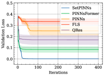
Figure 3: SetPINNs achieve faster convergence as well as the global minimum as opposed to other PINN approaches. Plotted is the validation loss vs. the number of training iterations.

The performance gains of SetPINNs can be attributed to their ability to model dependencies between neighboring points within the physical domain. Unlike traditional PINNs that rely on point-wise predictions, SetPINNs leverage the set-based approach to capture the implicit dependencies in the domain. This approach aligns with the principles of FEM, where interactions between elements are naturally considered, leading to more accurate and stable solutions.

A significant challenge in traditional PINNs is the tendency to converge to overly smooth and trivial solutions, particularly when dealing with PDEs that exhibit high-frequency or multi-scale features. As illustrated in Figure 1, existing PINN approaches often fail to approximate the true solution, resulting in smooth approximations that diverge from the actual behavior of the system. SetPINNs address this issue by incorporating dependencies between neighboring points within a set, effectively capturing the local interactions and variations that are critical for accurately modeling complex physical phenomena. By processing these sets using an attention mechanism, SetPINNs can focus on relevant features and relationships, avoiding the pitfall of trivial solutions. This is also evident in Figure 3, which shows that SetPINNs achieves faster convergence and a global minimum, whereas the other methods fail to do so.

By effectively incorporating physical constraints and leveraging set-based learning, SetPINNs can model intricate behaviors with high accuracy and are robust against failure modes across a diverse range of physical systems, making them a valuable tool for industrial and scientific applications.

6 Conclusion

In summary, we have introduced SetPINNs, a novel approach that improves PINNs using the idea of traditional FEM. Our method addresses the limitations of mesh-based solvers and traditional PINNs by being completely data-driven, mesh-free, and capable of capturing dependencies among neighboring points, all while respecting physical constraints. SetPINNs leverage the attention mechanism to model dependencies within sets of input elements, ensuring permutation invariance and efficient computation.

Through a set-wise physics loss, SetPINNs enforce physical constraints more effectively than traditional point-wise PINN losses. This approach is theoretically grounded, easy to implement, and versatile, making it applicable across various domains, including temporal, spatial, and elemental data.

Our experiments demonstrate that SetPINNs outperform existing state-of-the-art PINN architectures, particularly in scenarios where high-frequency or multi-scale features challenge traditional methods. By avoiding trivial solutions and providing accurate approximations, SetPINNs prove to be more robust against the common failure modes of PINNs.

The results highlight the potential of SetPINNs to revolutionize the solving of PDEs in diverse systems, paving the way for more reliable and efficient physical simulations. Furthermore, our results highlight the potential of PINNs as grey-box models [24] in application scenarios where limited experimental data is available, setting a new state-of-the-art performance for the prediction of activity coefficients. Future work could improve the discretization and sampling method for the points in the sets. Eventually, we expect that well-constructed hybrids of PINNs and FEM could lead to better speed and accuracy than FEM alone, especially for higher-dimensional problems.

Appendix A Proof

A.1 Definitions and Setup

Consider the PDE:

$$u_{t}+\mathcal{N}[u]=0,$$

where:

• $u(x,t)$: The unknown solution function dependent on spatial variable $x\in\Omega$ and time $t\in[0,T]$.

• $u_{t}$: Partial derivative of $u$ with respect to time $t$.

• $\mathcal{N}[u]$: A nonlinear operator acting on $u$. This could represent various physical phenomena like diffusion, advection, or reaction.

Finite Element Method (FEM)

The Finite Element Method (FEM) is a numerical approach for solving partial differential equations (PDEs) by approximating the solution space with a finite-dimensional subspace. The method operates over a spatial domain denoted as $\Omega$, where the domain is discretized into smaller subdomains called elements. The solutions within these elements are approximated using basis functions, $\phi_{i}(x)$, which are typically piecewise polynomials with local support; these functions are nonzero only over small regions of $\Omega$. The approximate solution, $u_{h}(x,t)$, is represented as a linear combination of these basis functions weighted by time-dependent coefficients, expressed mathematically as $u_{h}(x,t)=\sum_{i=1}^{N}U_{i}(t)\phi_{i}(x)$, where $U_{i}(t)$ are the coefficients and $\phi_{i}(x)$ the spatial basis functions. A common approach within FEM, the Galerkin Method, involves making the residual of the PDE orthogonal to the subspace spanned by these basis functions, thereby transforming the PDE into a system of ordinary differential equations (ODEs).

A.2 Proof

We now show that solutions $u_{h}(x_{1},t_{1})$ and $u_{h}(x_{2},t_{2})$ approximated by the FEM at two close points $(x_{1},t_{1})$ and $(x_{2},t_{2})$ are implicitly coupled through their shared basis functions.

Using the Galerkin method, we project the PDE onto the subspace spanned by the basis functions $\{\phi_{j}\}$:

$$\int_{\Omega}\phi_{j}(x)\left(\frac{\partial u_{h}}{\partial t}+\mathcal{N}[u_{h}]\right)\,dx=0\quad\forall j=1,\dots,N$$

Substituting the approximate solution:

$$\int_{\Omega}\phi_{j}(x)\left(\sum_{i=1}^{N}\frac{dU_{i}(t)}{dt}\phi_{i}(x)+\mathcal{N}\left[\sum_{i=1}^{N}U_{i}(t)\phi_{i}(x)\right]\right)\,dx=0$$

This leads to a system of ODEs for the coefficients $U_{i}(t)$:

$$\sum_{i=1}^{N}M_{ji}\frac{dU_{i}(t)}{dt}+\mathcal{N}_{j}(U)=0\quad\forall j,$$

where $M_{ji}=\int_{\Omega}\phi_{j}(x)\phi_{i}(x)\,dx$ is the mass matrix and $\mathcal{N}_{j}(U)=\int_{\Omega}\phi_{j}(x)\mathcal{N}[u_{h}]\,dx$.

The coefficients $U_{i}(t)$ determine the approximate solution $u_{h}(x,t)$. The basis functions $\phi_{i}(x)$ typically have local support, meaning each $\phi_{i}(x)$ is nonzero only over a small region of $\Omega$. However, the coefficients $U_{i}(t)$ are global in nature because the PDE and the Galerkin method couple them through the integrals over the entire domain $\Omega$.

Spatial Dependency

Since the basis functions overlap with neighboring elements, the value of $u_{h}(x,t)$ at any point $x$ is influenced by the coefficients $U_{i}(t)$ of the basis functions that overlap at $x$. Thus, $u_{h}(x_{1},t_{1})$ and $u_{h}(x_{2},t_{2})$ share some of the same coefficients $U_{i}(t)$ if $x_{1}$ and $x_{2}$ are close.

Temporal Dependency

The system of ODEs for $U_{i}(t)$ ensures that the coefficients evolve together over time. Hence, the solutions at different times $t_{1}$ and $t_{2}$ are coupled through the time integration of these ODEs.

Appendix B Experimentals

B.1 PDE Setup

For the PDE Setup, we follow the setup of Zhao et al. [46], as it is standard, diverse, and challenging.

Convection

The convection equation in one-dimensional space is characterized as a hyperbolic PDE, predominantly utilized for modeling the transport of quantities. It is described using periodic boundary conditions as:

$$\frac{\partial u}{\partial t}+\beta\frac{\partial u}{\partial x}=0,\quad\text{for }x\in[0,2\pi],\,t\in[0,1]$$ (8)

IC: $$\quad u(x,0)=\sin(x)$$

BC: $$\quad u(0,t)=u(2\pi,t)$$

In this setup, $\beta$ symbolizes the convection coefficient. Here, $\beta=50$ is chosen to observe the impact on the solution’s frequency.

1D Reaction

The one-dimensional reaction PDE, another hyperbolic PDE, is employed to simulate chemical reaction processes. It employs periodic boundary conditions defined as:

$$\frac{\partial u}{\partial t}-\rho u(1-u)=0,\quad\text{for }x\in[0,2\pi],\,t\in[0,1]$$ (9)

IC: $$\quad u(x,0)=\exp\left(-\frac{(x-\pi)^{2}}{2(\pi/4)^{2}}\right)$$

BC: $$\quad u(0,t)=u(2\pi,t)$$

$\rho$, the reaction coefficient, is set at 5, and the equation’s solution is given by:

$$u_{\text{analytical}}=\frac{h(x)\exp(\rho t)}{h(x)\exp(\rho t)+1-h(x)}$$ (10)

where $h(x)$ is based on the initial condition.

1D Wave

The one-dimensional wave equation, another hyperbolic PDE, is utilized across physics and engineering for describing phenomena such as sound, seismic, and electromagnetic waves. Periodic boundary conditions and system definitions are:

$$\frac{\partial^{2}u}{\partial t^{2}}-\beta\frac{\partial^{2}u}{\partial x^{2}}=0,\quad\text{for }x\in[0,1],\,t\in[0,1]$$ (11)

IC: $$\quad u(x,0)=\sin(\pi x)+\frac{1}{2}\sin(\beta\pi x),\quad\frac{\partial u(x,0)}{\partial t}=0$$

BC: $$\quad u(0,t)=u(1,t)=0$$

Here, $\beta$, representing the wave speed, is set to 3. The analytical solution is formulated as:

$$u(x,t)=\sin(\pi x)\cos(2\pi t)+\frac{1}{2}\sin(\beta\pi x)\cos(2\beta\pi t)$$ (12)

Navier-Stokes

The Navier-Stokes equations in two dimensions describe the flow of incompressible fluids and are a central model in fluid dynamics. These parabolic PDEs are formulated as follows:

$$\frac{\partial u}{\partial t}+\lambda_{1}\left(u\frac{\partial u}{\partial x}+v\frac{\partial u}{\partial y}\right) =-\frac{\partial p}{\partial x}+\lambda_{2}\left(\frac{\partial^{2}u}{\partial x^{2}}+\frac{\partial^{2}u}{\partial y^{2}}\right)$$ (13)

$$\frac{\partial v}{\partial t}+\lambda_{1}\left(u\frac{\partial v}{\partial x}+v\frac{\partial v}{\partial y}\right) =-\frac{\partial p}{\partial y}+\lambda_{2}\left(\frac{\partial^{2}v}{\partial x^{2}}+\frac{\partial^{2}v}{\partial y^{2}}\right)$$ (14)

Here, $u(t,x,y)$ and $v(t,x,y)$ represent the fluid’s velocity components in the x and y directions, and $p(t,x,y)$ is the pressure field. For this study, $\lambda_{1}=1$ and $\lambda_{2}=0.01$ are selected. The system does not have an explicit analytical solution, but the simulated solution is provided by [29].

B.2 Hyperparameters

Model hyperparameters.

Table 3 outlines the hyperparameters for the different models evaluated in this study, including Physics-Informed Neural Networks (PINNs), Quadratic Residual Networks (QRes), First-Layer Sine (FLS), PINNsFormer, and SetPINNs. Each model is configured with a specific number of hidden layers and hidden sizes. The PINNsFormer and SetPINNs models also include additional parameters such as the number of encoders and decoders, embedding size, and the number of attention heads. These configurations are crucial for defining the model architectures and their capacities to learn from the data. Table 4 shows the total parameters of all models. For a fair comparison, all models have relatively similar numbers of trainable parameters. For implementation, we follow the same implementation pipeline as of PINNsFormer and use their implementation of PINNs, QRes, FLS, and PINNsFormer. For fair comparisons, the model architecture of SetPINNs is kept consistent with PINNsFormer.

Model	Hyperparameter	Value
PINNs	hidden layers	4
	hidden size	512
QRes	hidden layers	4
	hidden size	256
FLS	hidden layers	4
	hidden size	512
PINNsFormer	$k$	5
	$\Delta t$	1e-4
	# of encoder	1
	# of decoder	1
	embedding size	32
	head	2
	hidden size	512
SetPINNs	set size	4
	# of encoder	1
	# of decoder	1
	embedding size	32
	head	2
	hidden size	512

Table 3: Hyperparameters for the different models evaluated in the study, including the number of hidden layers, hidden sizes, and additional parameters for complex models like PINNsFormer and SetPINNs.

Model	Total trainable parameters
PINNs	527K
FLS	527K
QRes	397K
PINNsFormer	454K
SetPINNs	454K

Table 4: Total number of trainable parameters for all models. For a fair comparison, all models have relatively similar numbers of trainable parameters.

Training hyperparameters.

The training process for the models utilized specific hyperparameters as listed in Table 5. The optimization involved a combination of the Adam optimizer and the L-BFGS optimizer, with a set number of iterations for each. Additionally, the line search function used in the L-BFGS optimization was the strong Wolfe condition. Parameters $\lambda_{f}$ and $\lambda_{u}$ were set to specific values to control the weighting of residual points and boundary points, respectively. These parameters were kept consistent across all models for a fair comparison. These training parameters were chosen to ensure efficient and effective convergence of all models during training.

Hyperparameter	Value
Adam Iterations	100
L-BFGS Iterations	1000
L-BFGS line search function	strong wolfe
$\lambda_{f}$	1
$\lambda_{u}$	1
train:val:test	50:21:101

Table 5: Training hyperparameters used for the models, including the number of iterations for the Adam and L-BFGS optimizers, the line search function, and the weighting parameters $\lambda_{f}$ and $\lambda_{u}$. These parameters were kept consistent across all models to ensure fair comparison and effective convergence.

B.3 Compute

All models are implemented in PyTorch, and are trained separately on single NVIDIA Tesla V100 GPU. In general, with hyperparameters mentioned in Appendix B.2 the runtime for one run using PINNs, FLS, QRes, PINNsFormer, and SetPINNs were: 103, 89, 149, 308, and 215 seconds respectively. The memory utilization of GPUs are provided in Table 6.

Compute	Value
SetPINNs GPU Memory (set size = 4)	1.8MiB
PINNs GPU Memory	2.1MiB
FLS GPU Memory	2.1MiB
QRes GPU Memory	1.6MiB
PINNsFormer GPU Memory	1.8MiB

Table 6: Approximate memory utilization by each model.

B.4 Training and Evaluation

Training Algorithm.

The training algorithm for SetPINNs, outlined in Algorithm 1, involves initializing the model parameters for the Set Generator, Mixer Network, Set Processor, and PDE Probe. During each training iteration, the algorithm processes each element in the discretized domain by sampling points to generate a set, transforming this set into a high-dimensional space using the Mixer Network, and then processing it with the Set Processor. The transformed set is used by the PDE Probe to predict solutions. The set-wise physics loss, defined in Equation 7, is computed to ensure adherence to physical laws. The model parameters are updated iteratively using the Adam optimizer, followed by fine-tuning with the L-BFGS optimizer, to achieve efficient and accurate convergence. This approach leverages set-based processing and transformer networks to simultaneously approximate solutions for multiple points in the domain.

Algorithm 1 Training Algorithm for SetPINNs

0:  Domain $\Omega$ discretized into $N$ elements $\{\Omega_{e}\}_{e=1}^{N}$

0:  Set Generator

0:  Mixer Network $p_{\psi}$

0:  Set Processor $f_{\phi}$

0:  PDE Probe $q_{\eta}$

0:  Hyperparameters $\lambda_{f}$, $\lambda_{u}$

1:  Initialize model parameters $\psi$, $\phi$, $\eta$

2:  for each training iteration do

3:     for each element $\Omega_{e}$ do

4:        Sample $K_{e}$ points from $\Omega_{e}$ to generate set $\mathcal{S}_{e}$

5:        Transform $\mathcal{S}_{e}$ into high-dimensional space $\mathcal{M}_{e}$ using Mixer Network $p_{\psi}$

6:        Process set $\mathcal{M}_{e}$ and obtain $\mathcal{O}_{e}$ using Set Processor $f_{\phi}$

7:        Predict solutions $u_{e}$ using PDE Probe $q_{\eta}$

8:     end for

9:     Compute set-wise physics loss as defined in Equation 7

10:     Update model parameters $\psi$, $\phi$, $\eta$

11:  end for

Evaluation.

The performance of the models was evaluated using two key metrics: Relative Mean Absolute Error (rMAE) and Relative Root Mean Square Error (rRMSE). The rMAE metric, as defined in Equation 15, calculates the mean absolute difference between the predicted and actual values, normalized by the mean of the actual values. This metric provides insight into the average magnitude of prediction errors relative to the actual values. The rRMSE, defined in Equation 16, measures the square root of the mean squared differences between predicted and actual values, normalized by the root mean square of the actual values. Both metrics are essential for assessing the accuracy and robustness of the models’ predictions across different datasets and scenarios.

$$\text{rMAE}=\frac{\Sigma_{n=1}^{N}|\hat{y}_{n}-y_{n}|}{\Sigma_{n=1}^{N}|y_{n}|}$$ (15)

$$\text{rRMSE}=\sqrt{\frac{\Sigma_{n=1}^{N}|\hat{y}_{n}-y_{n}|^{2}}{\Sigma_{n=1}^{N}|y_{n}|^{2}}}$$ (16)

B.5 Predicting activity coefficients

Activity coefficients are a central thermodynamic property describing the behavior of components in mixtures. In determining the deviation from the ideal mixture, activity coefficients are fundamental for modeling and simulating reaction and separation processes, such as distillation, absorption, and liquid-liquid extraction. In a mixture, each component has an individual activity coefficient that highly depends on the molecular structure of the components as well as on the temperature and concentration in the mixture (the latter is typically given in mole fractions of the components ranging between 0 and 1).

Since measuring activity coefficients is exceptionally time-consuming and expensive, experimental data on this property is scarce. Therefore, prediction methods are established in practice; the most commonly used ones are based on physical theories. Compared to machine-learning models for predicting activity coefficients, which have also been proposed in the literature [17], the most significant advantage of physical models is that they comply with thermodynamic consistency criteria, such as the Gibbs-Duhem equation that relates the activity coefficients within a mixture. For binary mixtures composed of two components and the isothermal and isobaric case, the Gibbs-Duhem equation reads:

$$x_{1}\left(\frac{\partial\text{ln}\gamma_{1}}{\partial x_{1}}\right)_{T}+(1-x_{1})\left(\frac{\partial\text{ln}\gamma_{2}}{\partial x_{1}}\right)_{T}=0$$ (17)

, where $\text{ln}\gamma_{1}$ and $\text{ln}\gamma_{2}$ are the logarithmic activity coefficients of the two components that make up the mixture, $T$ is the temperature, and $x_{1}$ is the mole fraction of the first component.

Setup.

The experimental activity coefficient data set was taken from the Dortmund Data Bank (DDB). Data on activity coefficients at infinite dilution were directly adopted from the DDB. Furthermore, activity coefficients were calculated from vapor-liquid equilibrium data from the DDB. In the preprocessing, data points labeled as poor quality by the DDB were excluded. Furthermore, only components for which a SMILES (simplified molecular-input line-entry system) string could be retrieved using the CAS number (preferred) or the component name using the Cactus database were considered. SMILES are a chemical language used to describe the molecular structure of a molecule. These SMILES were then converted into canonical SMILES using RDKit, which resulted in dropping a few SMILES that could not be converted. One system is defined as the combination of two components. The train-test split was done in a system-wise manner, whereby 10 % of the systems were used for the test set. RDKit was used to create molecular descriptors for each component. Specifically, a count-based Morgan fingerprint with zero radius and bitesize of 128 was used.

B.6 Predicting agglomerate breakage

Population balance equations (PBE) are a well-known and general method for calculating the temporal evolution of particle property distributions $u(x,t)$, with ever-increasing applications in a variety of fields [31]. In general, PBE are integro-differential equations and require numerical solutions. We investigate the one-dimensional case of pure agglomerate breakage, where analytical solutions exist for specific boundary conditions. The PBE is given by:

$$\frac{\partial u(x,t)}{\partial t}=\int\limits_{x}^{\infty}f(x,x^{\prime})r(x^{\prime})u(x^{\prime},t)\mathrm{d}x^{\prime}-r(x)u(x,t),$$ (18)

IC: $$\quad u(x,0)=\delta(x-L)$$

BC: $$\quad r(x)=x$$

$$\quad f(x,y)=\frac{2}{y}$$

Here, the breakage rate $r$ and breakage function $f$ are the so-called kernels and define the physical behavior of the system. The analytical solution for this special case is formulated as [49]:

$$u(x,t)=\mathrm{exp}\left(-tx\right)\left(\delta(x-L)+\left[2t+t^{2}(L-x)\right]\theta(L-x)\right)$$ (19)

with $\delta$ being dirac delta and

$$\theta(x-L)=\begin{cases}1,&x<L\\ 0,&\mathrm{otherwise}\end{cases}\quad.$$ (20)

In a real-world setting, i.e. when only experimental data is available, the kernel values are generally unknown. Although empirical equations exist, they have to be calibrated to experiments. This makes benchmarking solely on experimental data impossible and hence, we used the provided special case. However, it should be emphasized that PINNs have already been applied for solving the inverse problem, i.e. estimating unknown kernels [7]. Therefore, an improved accuracy on synthetic data will likely correspond to higher accuracy of the inverse problem, when applied to experimental data.

B.7 Ablation studies

In this section, we conduct a series of ablation studies to investigate the impact of various hyperparameters on the performance of SetPINNs. We examine the effects of different element sizes, the number of attention heads, and the number of transformer blocks in the encoder and decoder. For these ablation studies, we select a 1D reaction equation and use 100 residual, boundary, and initial points. The domain is discretized with a 100x100 grid, which is kept consistent across all experiments. All other hyperparameters remain the same unless specifically mentioned. We report rRMSE across all the experiments in ablation studies.

Element Size

In this experiment, we investigate the impact of varying element sizes on error rates. For this purpose, we use SetPINNs with hyperparameters specified in Table 3. Although we focus on simple square elements, the approach can be extended to elements of different shapes. The domain is partitioned into elements of size $n\times n$, from which discretized points are used to construct the set. Consequently, a $2\times 2$ element yields a set size of 4, a $4\times 4$ element yields a set size of 16, and so forth.

The results, depicted in Figure 4, indicate that as element size increases, the error rate rises significantly. We attribute this trend to the increased distance between points within the set for larger elements. In smaller elements, such as $2\times 2$, points are closer together compared to those in larger elements. Notably, using a larger element size leads to poorer results as the distance between the points increases. This result complies with and validates Theorem 3.1.1. As the distance between points attending to each other increases, we observe a trend where performance deteriorates. Thus, this experiment empirically validates Theorem 3.1.1.

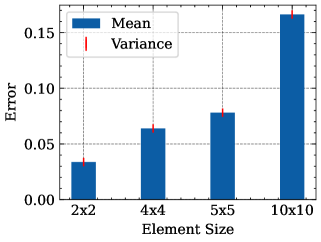
Figure 4: Bar chart illustrating the impact of element size on error rates. As shown, larger element sizes result in significantly higher error rates, which is attributed to the increased distance between points within the sets for larger elements. This trend empirically validates Theorem 3.1.1.

No of Transformer blocks

In this experiment, we explore the effect of varying the number of Transformer blocks on error rates. We conduct experiments using SetPINNs with hyperparameters specified in Table 3, testing configurations with both 1 and 2 Transformer blocks (N) in the encoder and decoder.

The results, depicted in Figure 5, show that using 2 transformer blocks significantly improves the results compared to using just 1 block. This improvement can be attributed to the additional layers providing more capacity for the model to learn complex representations, thereby enhancing performance.

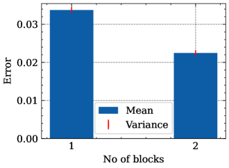
Figure 5: Bar chart illustrating the impact of the number of transformer blocks on error rates. The x-axis represents the number of transformer blocks in the encoder and decoder, and the y-axis shows the corresponding error rates. The results indicate that using 2 transformer blocks leads to significantly better performance compared to using just 1 block, likely due to the increased capacity for learning complex representations.

No of attention heads

In this experiment, we investigate the impact of varying no of attention heads on error rates. For this purpose, we utilize SetPINNs with hyperparameters outlined in Table 3, employing an embedding size of 256 instead of 32 to accommodate a greater number of heads.

The results, shown in Figure 6, reveal that the number of attention heads does not significantly impact error rates, as the error rates remain consistent across all experiments.rates remain similar across all the experiments. This could be because the increased number of attention heads does not provide additional useful representational capacity or because the model already captures the necessary information with fewer heads, leading to diminishing returns with more heads.

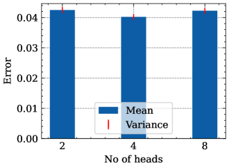
Figure 6: Bar chart illustrating the impact of varying the number of attention heads on error rates. The x-axis represents the number of attention heads, and the y-axis shows the corresponding error rates. The results indicate that changing the number of attention heads does not significantly affect the error rates, which remain consistent across different experiments. This suggests that the additional attention heads do not contribute to improved performance, possibly due to the model already capturing the necessary information with fewer heads.

Appendix C Limitations

While SetPINNs offer significant improvements in capturing the dependencies within physical systems and incorporating physical constraints, there are a few limitations to consider.

Firstly, the discretization and sampling of the points into sets are critical steps in the SetPINNs framework. The way in which these sets are generated can influence the performance of the model. Currently, this discretization and sampling process is simplistic and could benefit from more intelligent and adaptive methods (inspired by FEMs) that take into account the specific characteristics of the problem domain.

Secondly, the size and shape of the elements used in the discretization process act as hyperparameters that may need to be fine-tuned for different problems. As demonstrated in our ablation studies, varying these parameters can lead to varied results. This dependency implies that the optimal configuration of SetPINNs might vary from one application to another, requiring careful experimentation and adjustment for each new problem.

References

- [1] Rdkit: Open-source cheminformatics. (Last accessed: 04.04.2024). URL https://www.rdkit.org.
- DDB [2023] Dortmund data bank, 2023. URL https://www.ddbst.com/.
- Asylbekov et al. [2023] Ermek Asylbekov, Julian Mayer, Hermann Nirschl, and Arno Kwade. Modeling of carbon black fragmentation during high-intensity dry mixing using the population balance equation and the discrete element method. Energy Technology, 11(5):2200867, 2023. ISSN 2194-4288. doi: https://doi.org/10.1002/ente.202200867. URL https://doi.org/10.1002/ente.202200867.
- Bu and Karpatne [2021] Jie Bu and Anuj Karpatne. Quadratic residual networks: A new class of neural networks for solving forward and inverse problems in physics involving pdes. In Proceedings of the 2021 SIAM International Conference on Data Mining (SDM), pages 675–683. SIAM, 2021.
- Cai et al. [2021] Shengze Cai, Zhiping Mao, Zhicheng Wang, Minglang Yin, and George Em Karniadakis. Physics-informed neural networks (pinns) for fluid mechanics: A review. Acta Mechanica Sinica, 37(12):1727–1738, 2021.
- Chao et al. [2021] Hanqing Chao, Kun Wang, Yiwei He, Junping Zhang, and Jianfeng Feng. Gaitset: Cross-view gait recognition through utilizing gait as a deep set. IEEE transactions on pattern analysis and machine intelligence, 44(7):3467–3478, 2021.
- Chen et al. [2021a] Xizhong Chen, Li Ge Wang, Fanlin Meng, and Zheng-Hong Luo. Physics-informed deep learning for modelling particle aggregation and breakage processes. Chemical Engineering Journal, 426:131220, 2021a. ISSN 1385-8947. doi: https://doi.org/10.1016/j.cej.2021.131220. URL https://www.sciencedirect.com/science/article/pii/S1385894721028011.
- Chen et al. [2021b] Zhao Chen, Yang Liu, and Hao Sun. Physics-informed learning of governing equations from scarce data. Nature communications, 12(1):6136, 2021b.
- Daw et al. [2022] Arka Daw, Jie Bu, Sifan Wang, Paris Perdikaris, and Anuj Karpatne. Mitigating propagation failures in physics-informed neural networks using retain-resample-release (r3) sampling. arXiv preprint arXiv:2207.02338, 2022.
- Dhatt et al. [2012] Gouri Dhatt, Emmanuel Lefrançois, and Gilbert Touzot. Finite element method. John Wiley & Sons, 2012.
- Fredenslund et al. [1975] Aage Fredenslund, Russell L. Jones, and John M. Prausnitz. Group-contribution estimation of activity coefficients in nonideal liquid mixtures. AIChE Journal, 21(6):1086–1099, November 1975. ISSN 1547-5905. doi: 10.1002/aic.690210607. URL http://dx.doi.org/10.1002/aic.690210607.
- Fuks and Tchelepi [2020] Olga Fuks and Hamdi A Tchelepi. Limitations of physics informed machine learning for nonlinear two-phase transport in porous media. Journal of Machine Learning for Modeling and Computing, 1(1), 2020.
- Grossmann et al. [2023] Tamara G Grossmann, Urszula Julia Komorowska, Jonas Latz, and Carola-Bibiane Schönlieb. Can physics-informed neural networks beat the finite element method? arXiv preprint arXiv:2302.04107, 2023.
- Gundersen et al. [2021] Kristian Gundersen, Anna Oleynik, Nello Blaser, and Guttorm Alendal. Semi-conditional variational auto-encoder for flow reconstruction and uncertainty quantification from limited observations. Physics of Fluids, 33(1), 2021.
- Han et al. [2018] Jiequn Han, Arnulf Jentzen, and Weinan E. Solving high-dimensional partial differential equations using deep learning. Proceedings of the National Academy of Sciences, 115(34):8505–8510, 2018.
- Jeldres et al. [2015] Ricardo I. Jeldres, Fernando Concha, and Pedro G. Toledo. Population balance modelling of particle flocculation with attention to aggregate restructuring and permeability. Advances in Colloid and Interface Science, 224:62–71, 2015. ISSN 0001-8686. doi: https://doi.org/10.1016/j.cis.2015.07.009. URL http://www.sciencedirect.com/science/article/pii/S0001868615001153.
- Jirasek et al. [2020] Fabian Jirasek, Rodrigo AS Alves, Julie Damay, Robert A Vandermeulen, Robert Bamler, Michael Bortz, Stephan Mandt, Marius Kloft, and Hans Hasse. Machine learning in thermodynamics: Prediction of activity coefficients by matrix completion. The journal of physical chemistry letters, 11(3):981–985, 2020.
- Kingma and Ba [2014] Diederik P Kingma and Jimmy Ba. Adam: A method for stochastic optimization. arXiv preprint arXiv:1412.6980, 2014.
- Krishnapriyan et al. [2021] Aditi Krishnapriyan, Amir Gholami, Shandian Zhe, Robert Kirby, and Michael W Mahoney. Characterizing possible failure modes in physics-informed neural networks. Advances in Neural Information Processing Systems, 34:26548–26560, 2021.
- Lagaris et al. [1998] Isaac E Lagaris, Aristidis Likas, and Dimitrios I Fotiadis. Artificial neural networks for solving ordinary and partial differential equations. IEEE transactions on neural networks, 9(5):987–1000, 1998.
- Lee et al. [2019] Juho Lee, Yoonho Lee, Jungtaek Kim, Adam Kosiorek, Seungjin Choi, and Yee Whye Teh. Set transformer: A framework for attention-based permutation-invariant neural networks. In International conference on machine learning, pages 3744–3753. PMLR, 2019.
- Leiteritz and Pflüger [2021] Raphael Leiteritz and Dirk Pflüger. How to avoid trivial solutions in physics-informed neural networks. arXiv preprint arXiv:2112.05620, 2021.
- Lou et al. [2021] Qin Lou, Xuhui Meng, and George Em Karniadakis. Physics-informed neural networks for solving forward and inverse flow problems via the boltzmann-bgk formulation. Journal of Computational Physics, 447:110676, 2021.
- Manduchi et al. [2024] Laura Manduchi, Kushagra Pandey, Robert Bamler, Ryan Cotterell, Sina Däubener, Sophie Fellenz, Asja Fischer, Thomas Gärtner, Matthias Kirchler, Marius Kloft, et al. On the challenges and opportunities in generative ai. arXiv preprint arXiv:2403.00025, 2024.
- Mao et al. [2020] Zhiping Mao, Ameya D Jagtap, and George Em Karniadakis. Physics-informed neural networks for high-speed flows. Computer Methods in Applied Mechanics and Engineering, 360:112789, 2020.
- Mojgani et al. [2022] Rambod Mojgani, Maciej Balajewicz, and Pedram Hassanzadeh. Lagrangian pinns: A causality-conforming solution to failure modes of physics-informed neural networks. arXiv preprint arXiv:2205.02902, 2022.
- Psichogios and Ungar [1992] Dimitris C Psichogios and Lyle H Ungar. A hybrid neural network-first principles approach to process modeling. AIChE Journal, 38(10):1499–1511, 1992.
- Raissi [2018] Maziar Raissi. Deep hidden physics models: Deep learning of nonlinear partial differential equations. Journal of Machine Learning Research, 19(25):1–24, 2018.
- Raissi et al. [2019] Maziar Raissi, Paris Perdikaris, and George E Karniadakis. Physics-informed neural networks: A deep learning framework for solving forward and inverse problems involving nonlinear partial differential equations. Journal of Computational physics, 378:686–707, 2019.
- Raissi et al. [2020] Maziar Raissi, Alireza Yazdani, and George Em Karniadakis. Hidden fluid mechanics: Learning velocity and pressure fields from flow visualizations. Science, 367(6481):1026–1030, 2020.
- Ramkrishna and Singh [2014] Doraiswami Ramkrishna and Meenesh R. Singh. Population balance modeling: Current status and future prospects. Annual Review of Chemical and Biomolecular Engineering, 5:123–146, 2014. ISSN 19475438. doi: 10.1146/annurev-chembioeng-060713-040241.
- Schmidt [2005] Mark Schmidt. minfunc: unconstrained differentiable multivariate optimization in matlab. Software available at http://www. cs. ubc. ca/~ schmidtm/Software/minFunc. htm, 2005.
- Serviansky et al. [2020] Hadar Serviansky, Nimrod Segol, Jonathan Shlomi, Kyle Cranmer, Eilam Gross, Haggai Maron, and Yaron Lipman. Set2graph: Learning graphs from sets. Advances in Neural Information Processing Systems, 33:22080–22091, 2020.
- Shin et al. [2020] Yeonjong Shin, Jerome Darbon, and George Em Karniadakis. On the convergence of physics informed neural networks for linear second-order elliptic and parabolic type pdes. arXiv preprint arXiv:2004.01806, 2020.
- Vaswani et al. [2017] Ashish Vaswani, Noam Shazeer, Niki Parmar, Jakob Uszkoreit, Llion Jones, Aidan N Gomez, Łukasz Kaiser, and Illia Polosukhin. Attention is all you need. Advances in neural information processing systems, 30, 2017.
- Verma et al. [2024] Yogesh Verma, Markus Heinonen, and Vikas Garg. ClimODE: Climate forecasting with physics-informed neural ODEs. In The Twelfth International Conference on Learning Representations, 2024. URL https://openreview.net/forum?id=xuY33XhEGR.
- Wagstaff et al. [2022] Edward Wagstaff, Fabian B Fuchs, Martin Engelcke, Michael A Osborne, and Ingmar Posner. Universal approximation of functions on sets. Journal of Machine Learning Research, 23(151):1–56, 2022.
- Wang et al. [2021a] Sifan Wang, Yujun Teng, and Paris Perdikaris. Understanding and mitigating gradient flow pathologies in physics-informed neural networks. SIAM Journal on Scientific Computing, 43(5):A3055–A3081, 2021a.
- Wang et al. [2021b] Sifan Wang, Yujun Teng, and Paris Perdikaris. Understanding and Mitigating Gradient Flow Pathologies in Physics-Informed Neural Networks. SIAM Journal on Scientific Computing, September 2021b. doi: 10.1137/20M1318043. URL https://epubs.siam.org/doi/10.1137/20M1318043. Publisher: Society for Industrial and Applied Mathematics.
- Wang et al. [2022] Sifan Wang, Xinling Yu, and Paris Perdikaris. When and why pinns fail to train: A neural tangent kernel perspective. Journal of Computational Physics, 449:110768, 2022.
- Wong et al. [2022] Jian Cheng Wong, Chin Chun Ooi, Abhishek Gupta, and Yew-Soon Ong. Learning in sinusoidal spaces with physics-informed neural networks. IEEE Transactions on Artificial Intelligence, 5(3):985–1000, 2022.
- Wu et al. [2020] Yutian Wu, Yueyu Wang, Shuwei Zhang, and Harutoshi Ogai. Deep 3d object detection networks using lidar data: A review. IEEE Sensors Journal, 21(2):1152–1171, 2020.
- Zaheer et al. [2017] Manzil Zaheer, Satwik Kottur, Siamak Ravanbakhsh, Barnabas Poczos, Russ R Salakhutdinov, and Alexander J Smola. Deep sets. Advances in neural information processing systems, 30, 2017.
- Zhang et al. [2023] Hengrui Zhang, Jie Chen, James M Rondinelli, and Wei Chen. Molsets: Molecular graph deep sets learning for mixture property modeling. arXiv preprint arXiv:2312.16473, 2023.
- Zhang et al. [2022] Jie Zhang, Chen Cai, George Kim, Yusu Wang, and Wei Chen. Composition design of high-entropy alloys with deep sets learning. npj Computational Materials, 8(1):89, 2022.
- Zhao et al. [2024] Zhiyuan Zhao, Xueying Ding, and B. Aditya Prakash. PINNsformer: A transformer-based framework for physics-informed neural networks. In The Twelfth International Conference on Learning Representations, 2024. URL https://openreview.net/forum?id=DO2WFXU1Be.
- Zhu et al. [2019] Yinhao Zhu, Nicholas Zabaras, Phaedon-Stelios Koutsourelakis, and Paris Perdikaris. Physics-constrained deep learning for high-dimensional surrogate modeling and uncertainty quantification without labeled data. Journal of Computational Physics, 394:56–81, 2019.
- Zienkiewicz et al. [2005] Olek C Zienkiewicz, Robert L Taylor, and Jian Z Zhu. The finite element method: its basis and fundamentals. Elsevier, 2005.
- Ziff and McGrady [1985] R. M. Ziff and E. D. McGrady. The kinetics of cluster fragmentation and depolymerisation. Journal of Physics A: Mathematical and General, 18(15):3027, 1985. ISSN 0305-4470. doi: 10.1088/0305-4470/18/15/026. URL https://dx.doi.org/10.1088/0305-4470/18/15/026.