Distinguishing black holes with and without spontaneous scalarization in Einstein-scalar-Gauss-Bonnet theories via optical features

Abstract

Spontaneous scalarization in Einstein-scalar-Gauss-Bonnet theory admits both vacuum-general relativity (GR) and scalarized hairy black holes as valid solutions, which provides a distinctive signature of new physics in strong gravity regime. In this paper, we shall examine the optical features of Gauss-Bonnet black holes with spontaneous scalarization, which is governed by the coupling parameter $\lambda$. We find that the photon sphere, critical impact parameter and innermost stable circular orbit all decrease as the increasing of $\lambda$. Using observable data from Event Horizon Telescope, we establish the upper limit for $\lambda$. Then we construct the optical appearances of the scalarized black holes illuminated by various thin accretions. Our findings reveal that the scalarized black holes consistently exhibit smaller shadow sizes and reduced brightness compared to Schwarzschild black holes. Notably, in the case of thin spherical accretion, the shadow of the scalarized black hole is smaller, but the surrounding bright ring is more pronounced. Our results highlight the observable features of the scalarized black holes, providing a distinguishable probe from their counterpart in GR in strong gravity regime.

I Introduction

Remarkable detection progress on gravitational waves (GWs) LIGOScientific:2016aoc ; LIGOScientific:2017vwq ; LIGOScientific:2020aai and black hole images EventHorizonTelescope:2019dse ; EventHorizonTelescope:2019uob ; EventHorizonTelescope:2019jan ; EventHorizonTelescope:2019ths ; EventHorizonTelescope:2019pgp ; EventHorizonTelescope:2019ggy ; EventHorizonTelescope:2022wkp ; EventHorizonTelescope:2022apq ; EventHorizonTelescope:2022wok ; EventHorizonTelescope:2022exc ; EventHorizonTelescope:2022urf ; EventHorizonTelescope:2022xqj means that we are entering an unprecedented era to test the physics in strong gravity regime. It has to be admitted that the effects of higher-order curvature terms are especially profound when one refers to strong field regime of gravity via detections of GWs and black hole shadows. Such terms probably lead to the well-known ghost problem Stelle:1976gc , but Gauss-Bonnet term is a counter-case which can be ghost-free. It contributes no dynamics to the field equations when it is minimally coupled with Einstein-Hilbert action, but considering this term to couple with a scalar field is a smart way to make it meaningful in four-dimensional spacetime. Thus, as a special scalar-tensor theory with higher derivatives Horndeski:1974wa ; Deffayet:2009mn , the Einstein-scalar-Gauss-Bonnet (EsGB) gravity involves in considerable interest. In particular, the introduction of this coupling could make the theories admit hairy compact objects such as black hole (see for examples Mignemi:1992nt ; Kanti:1995vq ; Torii:1996yi ; Kleihaus:2011tg ; Sotiriou:2013qea ; Ayzenberg:2014aka ; Kleihaus:2016dui ), thus, the no-hair theorem Bekenstein:1972ny ; Teitelboim:1972ps in classical general relativity (GR) becomes more controversial.

Over the past decade, the spontaneous scalarizations with particular coupling functions in EsGB theory are extensively investigated. In this framework, besides GR solutions with a trivial scalar field configuration, the scalarized hairy solutions for black holes Doneva:2017bvd ; Silva:2017uqg ; Antoniou:2017acq and other compact objects Damour:1993hw ; Doneva:2017duq ; Antoniou:2019awm ; Ibadov:2020btp could also exist, which indeed evade the no-hair theorem. In details, below a certain mass, the Schwarzschild black hole background may become linearly unstable in regions of strong curvature, and the scalarized branches emerge when the scalar field backreacts to the geometry Doneva:2017bvd . The hairy branches were also found physically favorable Blazquez-Salcedo:2020rhf ; Blazquez-Salcedo:2020caw ; Blazquez-Salcedo:2018jnn . To better understand the procedure of spontaneous scalarizations in EsGB theory, extensive studies have been carried on. The spontaneous scalarizations due to a coupling of a scalar field to Ricci scalar Herdeiro:2019yjy , and to the Maxwell term Herdeiro:2018wub ; Fernandes:2019rez were studied and in the presence of Chern-Simons invariant was studied in Brihaye:2018bgc . The spontaneous scalarization of asymptotically AdS/dS black holes with a negative/positive cosmological constant was extended in Bakopoulos:2018nui ; Brihaye:2019gla ; Bakopoulos:2019tvc ; Bakopoulos:2020dfg ; Lin:2020asf ; Guo:2020sdu ; Guo:2024vhq . The influences of horizon curvature and spacetime structure on black hole spontaneous scalarization were studied in Guo:2020zqm . Also in EsGB theory, the spin-induced black hole spontaneous scalarization, which is the outcome of linear tachyonic instability triggered by rapid rotation, was explored in Collodel:2019kkx ; Dima:2020yac ; Doneva:2020kfv ; Herdeiro:2020wei ; Berti:2020kgk ; Lara:2024rwa , and the dynamical process during the spontaneous scalarization was simulated in Liu:2022fxy .

On the observational side, it was addressed in Wong:2022wni that spontaneous scalarization provides a distinctive signature of new physics in the strong gravity regime for those black holes whose Schwarzschild radii is comparable to the new length scale $\lambda$ in the theory, and the theory is not easy to constrain. Even so, they used the GW events (GW190814 and GW151226) and examined the GW’s constraining power on EsGB theory that allows for the spontaneous scalarization of black holes. To our knowledge, the optical features of the black holes with spontaneous scalarization in this theory have not been elaborated. In this regard, we are especially interested in the following two issues: (i) Is the black hole shadow data published by the Event Horizon Telescope (EHT) helpful to constrain the EsGB theory with spontaneous scalarization? (ii) Can the photon rings, shadows and images of the scalarized Gauss-Bonnet black holes be distinguishable from those of their counterpart in GR?

The black hole shadow corresponds to light rays that neither go to infinity nor fall into the event horizon from the view of backward ray-tracing, but are trapped within the spacetime. For the Schwarzschild black hole, its shadow shows a perfect circle Synge:1966okc . When turning on the rotation, the shadow of Kerr black hole becomes deformed and presents $D$-shape Bardeen:1973tla . Even though the spacetime disclosed by these shadows is in good agreement with the prediction of Kerr black hole, it still leaves some space for theoretical parameters of Kerr-like or other black hole solutions in modified theories of gravity due to the observational uncertainties. So the shadows of various modified theories of gravity have been extensively discussed, see for examples Amarilla:2010zq ; Wei:2013kza ; Wang:2017hjl ; Dastan:2016vhb ; Wang:2018prk ; Kuang:2022ojj ; Meng:2023wgi ; Meng:2022kjs ; Addazi:2021pty ; Li:2020drn ; Kuang:2022xjp ; Kumar:2019pjp ; Shaikh:2021yux ; Vagnozzi:2022moj ; Sui:2023rfh ; Kuang:2024ugn and references therein.

In a realistic universe, the black holes are usually surrounded by accretion flows that determine the optical appearances of black holes. One should use general relativistic magnetohydrodynamics to simulate the complex astrophysical process between black hole and accretion flow and further extract the image of black hole EventHorizonTelescope:2019pcy . However, some simplified accretion toy models are enough to capture main characteristics of black hole images. For example, Gralla et al. considered the Schwarzschild black hole illuminated by an optically and geometrically thin accretion disk Gralla:2019xty . By the number ($m$) of intersections between photon and accretion disk, they classified the emission types of light rays emitted from the accretion disk: direct ($m=1$), lensed ring ($m=2$) and photon ring ($m\geq 3$) emissions. The results showed that the direct emission determines the dominant contribution to the total observed brightness, followed by lensed ring emission, and photon ring emission can almost be ignored Gralla:2019xty . Moreover, when considering another kind of accretion, namely spherical accretion, the corresponding shadows are usually influenced by the spacetime geometry rather than the details of the accretions Falcke:1999pj ; Narayan:2019imo . So far, the observational appearances of black holes surrounded by various accretions have attracted much more attentions in modified theories of gravity Johnson:2019ljv ; Zeng:2020dco ; Zeng:2020vsj ; Peng:2020wun ; Qin:2020xzu ; Chakhchi:2022fls ; Guo:2021bhr ; Hu:2022lek ; Wen:2022hkv ; Meng:2024puu ; Gao:2023mjb ; Wang:2023vcv ; Chen:2023qic ; Yang:2024utv . Specially and importantly, the recent studies showed that the photon ring of black hole image could produce strong and universal signatures on long interferometric baselines Johnson:2019ljv . It is feasible to measure the structures of photon ring precisely through the analysis of interferometric signatures in black hole images.

Thus, in this paper, we will study the light rays around the scalarized Gauss-Bonnet black hole by using ray-tracing method. We will show the photon rings and images of the scalarized Gauss-Bonnet black hole illuminated by the optically and geometrically static thin accretion disk and spherical accretion, respectively. Based on the observational differences, we explore the potential method in strong field regime to distinguish the black hole with and without spontaneous scalarization by using black hole shadows and images. The remaining of this paper is organized as follows. In Sec.II, we give a brief review on Gauss-Bonnet black hole with spontaneous scalarization in EsGB theory. In Sec.III, we calculate the radius and critical impact parameter of the photon sphere for the scalarized black hole and give the constrains on the coupling parameter by utilizing the current black hole shadows data. In Sec.IV, we classify the light rays based on the trajectories of photons outside the scalarized black hole and investigate the optical appearances of scalarized black holes illuminated by the optically and geometrically thin accretion disk. In Sec.V, we consider the scalarized black hole surrounded by the static spherical accretion and show the optical appearances. Finally, we conclude our findings in Sec.VI.

II A quick review on scalarized Gauss-Bonnet black hole

We consider four dimensional EsGB theory with the action Doneva:2017bvd

$$S=\frac{1}{16\pi}\int d^{4}x\sqrt{-g}\Big{[}R-2\nabla_{\mu}\varphi\nabla^{\mu}\varphi+\lambda^{2}F(\varphi){\cal R}^{2}_{\text{GB}}\Big{]},$$ (1)

where $R$ is the Ricci scalar, $\varphi$ is the scalar field and ${\cal R}^{2}_{\text{GB}}=R^{2}-4R^{\mu\nu}R_{\mu\nu}+R^{\mu\nu\alpha\beta}R_{\mu\nu\alpha\beta}$ is the Gauss-Bonnet invariant. $F(\varphi)$ is the scalar coupling function which is non-minimally coupled to Gauss-Bonnet term. Thus, $\lambda$ is the Gauss-Bonnet coupling parameter that has the dimension of length. When $\lambda=0$ and $\varphi=\text{const.}$, this theory will recover to GR. By varying the action (1) with respect to the metric tensor $g_{\mu\nu}$ and the scalar field $\varphi$, we can derive the following fields equations Doneva:2017bvd

$$R_{\mu\nu}-\frac{1}{2}Rg_{\mu\nu}+\Gamma_{\mu\nu}=2\nabla_{\mu}\varphi\nabla_{\nu}\varphi-g_{\mu\nu}\nabla_{\alpha}\varphi\nabla^{\alpha}\varphi,$$ (2)

$$\nabla_{\alpha}\nabla^{\alpha}\varphi=-\frac{\lambda^{2}}{4}\frac{dF(\varphi)}{d\varphi}{\cal R}^{2}_{\text{GB}},$$ (3)

where the symbol $\Gamma_{\mu\nu}$ is defined by

$$\Gamma_{\mu\nu} = -R(\nabla_{\mu}\Psi_{\nu}+\nabla_{\nu}\Psi_{\mu})-4\nabla^{\alpha}\Psi_{\alpha}\left(R_{\mu\nu}-\frac{1}{2}Rg_{\mu\nu}\right)+4R_{\mu\alpha}\nabla^{\alpha}\Psi_{\nu}+4R_{\nu\alpha}\nabla^{\alpha}\Psi_{\mu}$$ (4)

$$-4g_{\mu\nu}R^{\alpha\beta}\nabla_{\alpha}\Psi_{\beta}+\,4R^{\beta}_{\;\mu\alpha\nu}\nabla^{\alpha}\Psi_{\beta},$$

with $\Psi_{\mu}=\lambda^{2}\frac{dF(\varphi)}{d\varphi}\nabla_{\mu}\varphi$. Just like in GR, the above field equations are of second-order and the theory is free from ghosts . It was shown that the theory will result in GR equation with standard Klein-Gordon (KG) equation and admits scalar-free GR solutions when the coupling function $F(\varphi)$ satisfies the conditions $\frac{dF}{d\varphi}\big{|}_{\varphi=0}=0$ and $\varphi=0$ Doneva:2017bvd . Considering the scalar perturbation $\delta\varphi$ around the GR solution, the linearized KG equation (3) reads

$$\left(\square_{(0)}-m^{2}_{\text{eff}}\right)\delta\varphi=0,$$ (5)

where $m^{2}_{\text{eff}}=-\frac{\lambda^{2}}{4}\frac{d^{2}F}{d\varphi^{2}}\big{|}_{\varphi=0}{\cal R}^{2}_{\text{GB}(0)}$ is effective mass squared of the scalar perturbation $\delta\varphi$ and the subscript “0” represents the GR background geometry. It was shown that the negative effective mass triggers a tachyonic instability, the scalar-free GR solution is unstable and the BH solutions with nontrivial scalar field will be produced spontaneously Doneva:2017bvd . That is the spontaneous scalarization of BH induced by the curvature of the spacetime Doneva:2017bvd ; Silva:2017uqg we will focus on, which is different from that sourced by matters Cardoso:2013fwa ; Cardoso:2013opa .

Next we will closely follow the steps described in Doneva:2017bvd to construct the scalarized black hole solutions. We consider the following ansatz to construct the static, spherically symmetric and asymptotically flat spacetime and assume that the scalar field has the same symmetric configurations with the spacetime given by

$$ds^{2}=-h(r)dt^{2}+\frac{1}{f(r)}dr^{2}+r^{2}\left(d\theta^{2}+\text{sin}^{2}\theta d\phi^{2}\right),\qquad\varphi=\varphi(r).$$ (6)

The asymptotic flatness requires the metric functions and scalar field to behave as

$$h(r)=1-\frac{2M}{r}+\cdots,\quad f(r)=1-\frac{2M}{r}+\cdots,\quad\varphi(r)=\varphi_{\infty}+\frac{D}{r}+\cdots,$$ (7)

where $M$ and $D$ are the Arnowitt-Deser-Misner mass and scalar charge, respectively, and the constant of scalar field at infinity, $\varphi_{\infty}$, can be chosen as zero. Moreover, the existence of event horizon requires $h(r)|_{r\rightarrow r_{h}}\rightarrow 0$ and $f(r)|_{r\rightarrow r_{h}}\rightarrow 0$, while the regularity of scalar field near the event horizon directly gives

$$\left(\frac{d\varphi}{dr}\right)_{h}=\frac{r_{h}}{4\lambda^{2}\frac{dF}{d\varphi}(\varphi_{h})}\left[-1\pm\sqrt{1-\frac{24\lambda^{4}}{r^{4}_{h}}\left(\frac{dF}{d\varphi}(\varphi_{h})\right)^{2}}\right],$$ (8)

where the subscript $h$ indicates the physical quantities evaluated at the event horizon. Note that one has to choose the plus sign, since only in this case can we recover the Schwarzschild solution in the limit $\varphi_{h}\rightarrow 0$. Meanwhile, the above equation implies that the black hole with a nontrivial scalar field can exist only when

$$r_{h}^{4}>24\lambda^{4}\left(\frac{dF}{d\varphi}(\varphi_{h})\right)^{2}.$$ (9)

Thus, one can solve the field equations with the aforementioned boundary conditions to find the scalarized black hole solutions, once the formula of coupling function $F(\varphi)$ is given. A quite similar choice in the spontaneous scalarization of neutron stars Damour:1993hw

$$F(\varphi)=\frac{1}{12}\left(1-e^{-6\varphi^{2}}\right),$$ (10)

was found to lead the significant deviations from the Schwarzschild solution and the condition (9) is satisfied for a large enough range of parameters Doneva:2017bvd . It is noted that in the following study, we will rescale the quantities $(r,\lambda,D,M)$ of this system into the dimensionless ones $(r/M,\lambda/M,D/M,1)$. The numerical results of the scalar charge $D$ and scalar field at the event horizon $\varphi_{h}$ as functions of the coupling parameter are plotted in Fig.1 . From this figure, one can find that when the coupling $\lambda$ is small, the scalar field is trivial, implying the Schwarzschild black hole solution. When the coupling is larger than a critical value ($\lambda/M\approx 1.7$ agrees well with that found in Doneva:2017bvd ), nontrivial scalar field emerges, indicating that the scalarized black holes exist due to the spontaneous scalarization of the Schwarzschild black hole. Samples of profiles of the scalarized black hole metric and the nontrivial scalar field are depicted in Fig.2 where we also exhibit the Schwarzschild case for comparison. It is obvious that the scalarized black holes deviate significantly from the Schwarzschild solution, but they share the same flat asymptotic behavior.

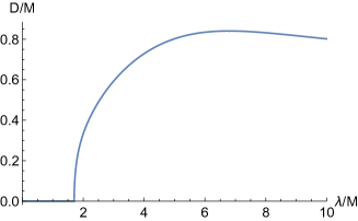
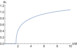
Figure 1: The scalar charge $D$ and the scalar field at the event horizon $\varphi_{h}$ as the functions of coupling $\lambda$.

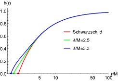
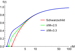
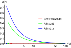
Figure 2: The metric and scalar fields functions as the functions of radial coordinate $r$ for different coupling $\lambda$. The color dots denote the positions of event horizon of corresponding coupling parameters.

Notably, Fig.2 only gives the first nontrivial branch of the scalarized solutions in which the scalar field has solo zero in the infinity, but many other nontrivial branches can exist in certain region of the parameter, depending on the number of zeros of the scalar field. However, the first nontrivial branch was found to be thermodynamically favorable over both their counterpart in GR and other branches, of which the metric profiles are also indistinguishable from Schwarzschild solution Doneva:2017bvd . Therefore, we will only focus on the first nontrivial branch of scalarized solutions to explore the effect of spontaneous scalarization on the optical features of black hole.

III Photon sphere of the scalarized Gauss-Bonnet black hole

In this section, we will investigate the radius and critical impact parameter of photon sphere for the scalarized Gauss-Bonnet black hole. The motions of photons are determined by the Euler-Lagrange equation

$$\frac{d}{d\tau}\left(\frac{\partial\mathcal{L}}{\partial\dot{x}^{\mu}}\right)=\frac{\partial\mathcal{L}}{\partial x^{\mu}},$$ (11)

where $\tau$ is the affine parameter and $\dot{x}^{\mu}=d{x}^{\mu}/d\tau$ denotes the four-velocity of the photon. For the metric (6), the Lagrangian of photons takes the following form

$$\mathcal{L}=\frac{1}{2}g_{\mu\nu}\dot{x}^{\mu}\dot{x}^{\nu}=\frac{1}{2}\left(-h(r)\dot{t}^{2}+\frac{1}{f(r)}\dot{r}^{2}+r^{2}\left(\dot{\theta}^{2}+\text{sin}^{2}\theta\dot{\phi}^{2}\right)\right).$$ (12)

Considering the time-translational and spherical symmetries of the spacetime, there exist two conserved quantities of photons which are the energy $E$ and angular momentum $L_{z}$ respectively given by

$$E\equiv-\frac{\partial\mathcal{L}}{\partial\dot{t}}=h(r)\dot{t},\qquad L_{z}\equiv\frac{\partial\mathcal{L}}{\partial\dot{\phi}}=r^{2}\text{sin}^{2}\theta\dot{\phi}.$$ (13)

Moreover, due to the spherical symmetries of the metric, it is convenient to only focus on the photons moving on the equatorial plane ($\theta=\pi/2$). Further, from the $\mathcal{L}=0$ for photons and impact parameter $b$ defined by $b\equiv L_{z}/E$, we can finally obtain three first-order differential equations that determine the photons’ motion in the spacetime written by

$$\dot{t}=\frac{1}{b\,h(r)},$$ (14)

$$\dot{\phi}=\pm\frac{1}{r^{2}},$$ (15)

$$\frac{h(r)}{f(r)}\dot{r}^{2}+V_{\text{eff}}(r)=\frac{1}{b^{2}},$$ (16)

with the effective potential

$$V_{\text{eff}}(r)=\frac{h(r)}{r^{2}}.$$ (17)

Note that the affine parameter $\tau$ has been redefined as $\tau/L_{z}$. The sign $``+"$ and $``-"$ denote that the photon moves on the equatorial plane along the counterclockwise and clockwise direction, respectively. From the Eq.(15) and Eq.(16), we can obtain the compact form for the equation of motion given by

$$\frac{dr}{d\phi}=\pm r^{2}\sqrt{\frac{f(r)}{h(r)}\left(\frac{1}{b^{2}}-V_{\text{eff}}(r)\right)}.$$ (18)

Obviously, the trajectory of photon is determined by the impact parameter $b$ and effective potential $V_{\text{eff}}$. When $dr/d\phi=0$, meaning $V_{\text{eff}}(r_{0})=1/b^{2}$. It implies that the photon approaches the black hole from infinity, and then moves towards infinity again after their distance reaching a minimum radius $r_{0}$. Further, there exists a critical value of $r_{0}$, smaller than which will make the photon fall into the black hole instead of escaping to infinity. This critical value is known as radius of photon sphere $r_{ph}$ that corresponds to the critical impact parameter $b_{ph}$, which is determined by $d^{2}r/d\phi^{2}=0$ combined with $dr/d\phi=0$. These two conditions of photon sphere will be finally translated to

$$V_{\text{eff}}(r_{ph})=\frac{1}{b_{ph}^{2}},\qquad V_{\text{eff}}^{\prime}(r_{ph})=0.$$ (19)

While for the massive particle, similar physical process gives the innermost stable circular orbit (ISCO), the radius of which for the particle orbiting the metric (6) can be evaluated by Wang:2023vcv

$$r_{isco}=\frac{3h(r_{isco})h^{\prime}(r_{isco})}{2h^{\prime}(r_{isco})^{2}-h(r_{isco})h^{\prime\prime}(r_{isco})}.$$ (20)

The radii of event horizon $r_{h}$, photon sphere $r_{ph}$, critical impact parameter $b_{ph}$, and ISCO $r_{isco}$ as the functions of coupling parameter $\lambda$ are shown in Fig.3. Samples of numerical results are listed in Table 1. We find that when the coupling parameter is increased from zero, these four physical quantities keep unchanged since the Schwarzschild black hole always keeps its own state in certain parameter region. When the increased coupling parameter is beyond critical coupling for the formation of spontaneous scalarization, these four physical quantities decrease monotonously.

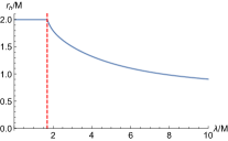
(a)   $r_{h}$

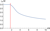
(b)   $r_{ph}$

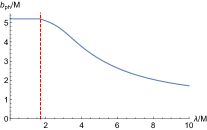
(c)   $b_{ph}$

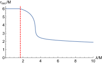
(d)   $r_{isco}$

Figure 3: The event horizon $r_{h}$, radius of photon sphere $r_{ph}$, critical impact parameter $b_{ph}$, and innermost stable circular orbit $r_{isco}$ as the functions of the coupling parameter $\lambda$. The vertical red dashed lines denote the critical coupling for the formation of spontaneous scalarization $\lambda/M=1.7$.

$\lambda/M$	Schwarzschild	$2$	$2.5$	$3$	$3.3$	$4$
$r_{h}/M$	2	1.79415	1.62264	1.50074	1.44096	1.32459
$r_{ph}/M$	3	2.8531	2.58255	2.23677	2.06705	1.81719
$b_{ph}/M$	5.19615	5.08947	4.88294	4.55848	4.31981	3.75795
$r_{isco}/M$	6	5.87473	5.61554	5.11077	4.41099	2.43372

Table 1: The numerical results of the event horizon $r_{h}$, radius of photon sphere $r_{ph}$, critical impact parameter $b_{ph}$ and innermost stable circular orbit $r_{isco}$ as the functions of the coupling parameter $\lambda$.

We analyze the motion of photon from the point of the effective potential as shown in the left figure of Fig.4. In Region 3 ($b>b_{ph}$), the photon from the infinity will be scattered into infinity after passing through the turning point. In Region 1 ($b<b_{ph}$), the photon will fall into the black hole. However for the critical situation in Region 2 ($b=b_{ph}$), the photon asymptotically approaches the photon sphere and then orbits around the black hole infinite times. These analyses are in good agreement with the trajectories of light rays by numerically solving Eq.(18). In the right figure of Fig.4, we show the effective potential for different coupling $\lambda$ and find that when increasing $\lambda$, the position of the effective potential’s peak moves left and the peak is improved, which implies the decreasing of $r_{h}$, $r_{ph}$ and $b_{ph}$ shown in Fig.3. Note that we scan the coupling parameter space of scalarized Gauss-Bonnet black hole and find that the effective potential always has a single-peak that indicates the existence of only one photon sphere. This is different from the scalarized Reissner-Nordström (RN) black hole Gan:2021pwu ; Gan:2021xdl and the hairy Schwarzschild black hole Meng:2023htc that will show the double-peak in the effective potential and lead to the structure of multiple photon spheres and more richer optical features.

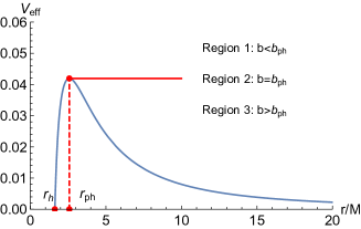
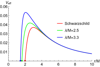
Figure 4: Left: The effective potential $V_{\text{eff}}$ as a function of radial coordinate $r$ for $\lambda/M=2.5$ as an example. Right: The effective potential as a function of radial coordinate $r$ for different $\lambda$, where the color dots denote the positions of event horizon of corresponding coupling parameters.

For a distant observer, the angular diameter $\theta_{d}$ of black hole shadow is measured by Kumar:2020owy

$$\theta_{d}=2\frac{b_{ph}}{d_{L}},$$ (21)

where $b_{ph}$ is the critical impact parameter and $d_{L}$ is the distance between the black hole and observer. We can use the observational data on the black hole shadow from the EHT to roughly constrain the coupling parameter $\lambda$. For the M87* black hole with the mass $M=6.5\times 10^{9}M_{\odot}$ and distance $d_{L}=16.8\,\text{Mpc}$ EventHorizonTelescope:2019dse , the angular diameter is roughly bounded between $29.32\,\mu as$ and $51.06\,\mu as$ EventHorizonTelescope:2021dqv ; Kuang:2022ojj . While for the Sgr A* black hole with the mass $M=4.0\times 10^{6}M_{\odot}$ and distance $d_{L}=8.15\,\text{kpc}$ EventHorizonTelescope:2022wkp , the angular diameter is $\theta_{d}=48.7\pm 7\,\mu as$ EventHorizonTelescope:2022wkp ; EventHorizonTelescope:2022xqj . Thus, the EHT data provides the constraints for the coupling parameter, and gives the upper limits $\lambda/M=3.89$ by M87* black hole and $\lambda/M=3.31$ by Sgr A* black hole, respectively (see Fig.5).

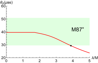
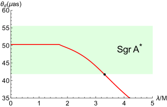
Figure 5: The constraints of the coupling parameter $\lambda$ by the observational shadows of M87* (Left) and Sgr A* black holes (Right). The black dots denote the upper limits for $\lambda$, which are $\lambda/M=3.89$ and $\lambda/M=3.31$, respectively.

IV Rings and images of scalarized Gauss-Bonnet black hole illuminated by thin disk accretions

In this section, we shall discuss the optical appearances of the scalarized Gauss-Bonnet black holes illuminated by the optically and geometrically thin accretion disks. We assume that the disk is located on the equatorial plane around the black hole and keeps rest, viewed face-on. To this end, based on the times that photons intersects with the accretion disk, we will firstly classify the light rays, which should contribute differently to the total observed intensity, and then explore the image of the scalarized black hole surrounded by three toy accretion disks.

IV.1 Classification of light rays: direct, lensed ring and photon ring emissions

For the certain impact parameter $b$ of the photon, one can obtain the complete trajectory of light ray by numerically solving Eq.(18), and also calculate the total change of azimuthal angle $\phi$ that the photon orbits the black hole. By defining the orbit number $n=\phi/(2\pi)$ proposed in Gralla:2019xty , we can classify the light rays into three types. The first type is called direct emission with $n<3/4$, where light ray intersects the accretion disk at most once. The second type with $3/4<n<5/4$ is lensed ring emission, where light ray crosses the accretion disk twice. The third type is photon ring emission where the light ray with $n>5/4$ crosses the accretion disk at least three times. Please refer to Hu:2022lek ; Wielgus:2021peu ; Bisnovatyi-Kogan:2022ujt for the schematic diagrams to help understand above descriptions.

The orbit numbers with respect to impact parameter $b$ for different coupling parameter $\lambda$ are shown in the top panel of Fig.6. Similar to that in Schwarzschild case, the scalarized Gauss-Bonnet black holes have a single-peak orbit number due to the single-peak effective potential indicating the single photon sphere. When increasing $\lambda$, the position of the peak moves towards the origin that indicates smaller photon sphere. Compared to the Schwarzschild black hole, the scalarized Gauss-Bonnet black holes have the wider ranges of impact parameter for both photon and lensed rings emissions, while the direct emission shrinks, which are also listed in Table.2. Moreover, we also present the photon trajectories in the polar coordinates in the bottom panel of Fig.6, which further verifies our above discussions.

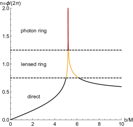
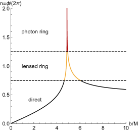
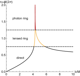
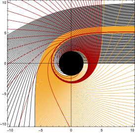
(a)   Schwarzschild

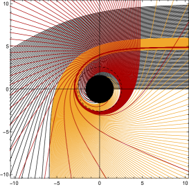
(b)   $\lambda/M=2.5$

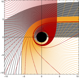
(c)   $\lambda/M=3.3$

Figure 6: The orbit numbers $n$ (Top) and trajectories of photons (Bottom) as the functions of impact parameter $b$ for different coupling $\lambda$. The black, gold, and red curves correspond to the direct ($n<3/4$), lensed ring ($3/4<n<5/4$), and photon ring ($n>5/4$) emissions respectively. The black hole is shown as the solid black disk and the photon sphere is denoted by a black dashed curve.

$\lambda/M$	Direct ($n<3/4$)	Lensed ring ($3/4<n<5/4$)	Photon ring ($n>5/4$)
Schwarzschild	$b<5.01514$ and $b>6.16757$	$5.01514<b<5.18781$ and $5.22794<b<6.16757$	$5.18781<b<5.22794$
$2.5$	$b<4.65037$ and $b>6.03995$	$4.65037<b<4.86696$ and $4.94237<b<6.03995$	$4.86696<b<4.94237$
$3.3$	$b<4.14904$ and $b>5.85411$	$4.14904<b<4.31176$ and $4.40013<b<5.85411$	$4.31176<b<4.40013$

Table 2: The ranges of impact parameter $b$ correspond to the direct, lensed ring, and photon ring emissions of the scalarized black hole for different coupling $\lambda$.

IV.2 Observed intensities and optical appearances

In the previous subsection, we have classified the light rays in terms of the times that photons intersects with the thin accretion disk. During the process of intersection, the photon will extract energy from the accretion disk each time Gralla:2019xty . Therefore different types of light rays will contribute differently to the total observed intensity. Moreover, the analysis in above subsection implies that compared to the Schwarzschild case, the spontaneous scalarization of black hole has a significant effect on the distribution of light rays. So in this section, we will further study the observed intensities and optical appearances of the scalarized Gauss-Bonnet black hole.

For simplicity, we assume that the accretion disk is optically and geometrically thin and emits isotropically in the rest frame of static worldlines. The specific intensity received by the observer with emission frequency $\nu_{e}$ is

$$I_{o}(r,\nu_{o})=g^{3}I_{e}(r,\nu_{e}),$$ (22)

where $g=\nu_{o}/\nu_{e}=\sqrt{h(r)}$ is the redshift factor Gan:2021pwu , and $I_{e}(r,\nu_{e})$ is the specific intensity of the accretion disk. By integrating all observed frequencies of $I_{o}(r,\nu_{o})$, the total observed intensity can be written as

$$I_{obs}(r)=\int I_{o}(r,\nu_{o})d\nu_{o}=\int g^{4}I_{e}(r,\nu_{e})d\nu_{e}=h(r)^{2}I_{em}(r),$$ (23)

where we denote $I_{em}(r)=\int I_{e}(r,\nu_{e})d\nu_{e}$ as the total emitted intensity, which is dependence of concrete emission profile. Based on our previous discussion, the photons that extract brightness once, twice or more to contribute to the total observed intensity depend on their impact parameter $b$. Therefore, the total observed intensity should be the sum of the intensities from each intersection read as

$$I_{obs}(b)=\sum_{m}h(r)^{2}I_{em}(r)|_{r=r_{m}(b)},$$ (24)

where we have introduced the transfer function $r_{m}(b)$ $(m=1,2,3,...)$. Physically, the transfer function, which transfers the brightness from accretion disk to the observer, establishes a one-to-one correspondence between the light ray’s impact parameter $b$ and the radial coordinate $r$ of the $m$-th intersection with the accretion disk. That is to say, if giving a impact parameter, one can directly obtain the brightness after using the transfer function by Eq.(24). We plot the first three transfer functions $r_{m}(b)$ for different coupling $\lambda$ in Fig.7. From these figures, we can find the following characteristics. For the first transfer function $(m=1)$, it corresponds to the direct image originating from direct, lensed and photon rings emissions. And its slope $dr/db$ that describes the demagnification factor at each $b$ Gralla:2019xty is almost 1 so this direct image is the source profile after redshift. For the second transfer function $(m=2)$, it originates from lensed and photon rings emissions and its slope is large. For the third transfer function $(m=3)$, it only originates from photon ring emission and has the extremely large slope. These properties mean that the first transfer function will play a leading contribution in the total brightness and other transfer functions contribute very little fluxes. Moreover, for the scalarized black hole, we find that the demagnification factors of the second and third transfer functions are suppressed by $\lambda$. It will lead to the wider range of the corresponding emission (that is impact parameter) than the Schwarzschild case, which agrees with the information from Table.2, and make them easier to be seen. Note that due to the extreme demagnification for higher-order transfer function $(m>3)$, it is enough for our illustrative purpose to consider the contributions of the first three transfer functions into total observed intensity.

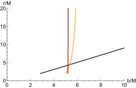
(a)   Schwarzschild

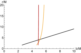
(b)   $\lambda/M=2.5$

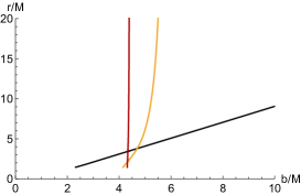
(c)   $\lambda/M=3.3$

Figure 7: The first three transfer functions in scalarized Gauss-Bonnet black hole for different $\lambda$. They represent the radial coordinate of the first (black), second (gold), and third (red) intersections with the emission disk.

Before figuring out the optical appearance of scalarized black hole, we need provide the emission function of the accretion disk $I_{em}(r)$ appeared in Eq.(24). Here we consider three toy-model emission functions Wang:2022yvi ; Yang:2022btw . Firstly, we assume that the emission of accretion disk is the square decay function that starts from the innermost stable circular orbit $r_{isco}$

$$\text{profile 1:}\quad I_{em}(r) :=\begin{cases}I_{0}\left[\frac{1}{r-(r_{isco}-1)}\right]^{2},&\hskip 31.2982ptr>r_{isco}\\ 0,&\hskip 31.2982ptr\leqslant r_{isco}\end{cases},$$ (25)

where $I_{0}$ is the maximum intensity (the same below). Secondly, the emission function starts from the photon sphere $r_{ph}$ and exhibit a cubic decay behaviour

$$\text{profile 2:}\quad I_{em}(r) :=\begin{cases}I_{0}\left[\frac{1}{r-(r_{ph}-1)}\right]^{3},&\hskip 32.72049ptr>r_{ph}\\ 0,&\hskip 32.72049ptr\leqslant r_{\rm ph}\end{cases}.$$ (26)

Thirdly, the emission function show more moderate decay than above two functions emitting from the event horizon $r_{h}$

$$\text{profile 3:}\quad I_{em}(r) :=\begin{cases}I_{0}\frac{\frac{\pi}{2}-\arctan[r-(r_{isco}-1)]}{\frac{\pi}{2}-\arctan[r_{h}-(r_{isco}-1)]},&\quad r>r_{h}\\ 0,&\quad r\leqslant r_{h}\end{cases}.$$ (27)

The sketches of three accretion disk emission profiles are explicitly drawn in Fig.8.

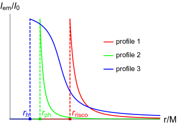
Figure 8: The sketches of three accretion disk emission profiles plotted by Eq.(25), Eq.(26), and Eq.(27) respectively.

Based on the given emission functions, we evaluate the total observed intensities for Schwarzschild and scalarized Gauss-Bonnet black holes, and then transfer them into the corresponding two-dimensional images, which are shown in Fig.9. For all cases, the results show that compared to Schwarzschild case, the scalarized black hole will show smaller shadow region and fainter brightness with the increasing of coupling $\lambda$. Especially, for the first emission profile of accretion disk, we find that the middle peak in the observed intensities has a larger width than Schwarzschild case (in fact the innermost peak is also like this and just hard to see). This is because the demagnification factors of the second and third transfer functions are suppressed by $\lambda$ and the range of the corresponding emission becomes wider, as discussed in the above. Obviously, this leads the second ring of scalarized black hole is more clear than Schwarzschild case in the image. Similarly, for the second and third emission profiles, the peaks of scalarized black hole in the observed intensities are also wider than Schwarzschild cases by $\lambda$, indicating a wider but dimmed photon ring in the corresponding image.

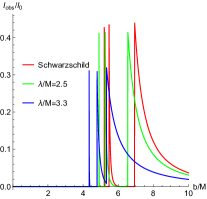
(a)   profile 1

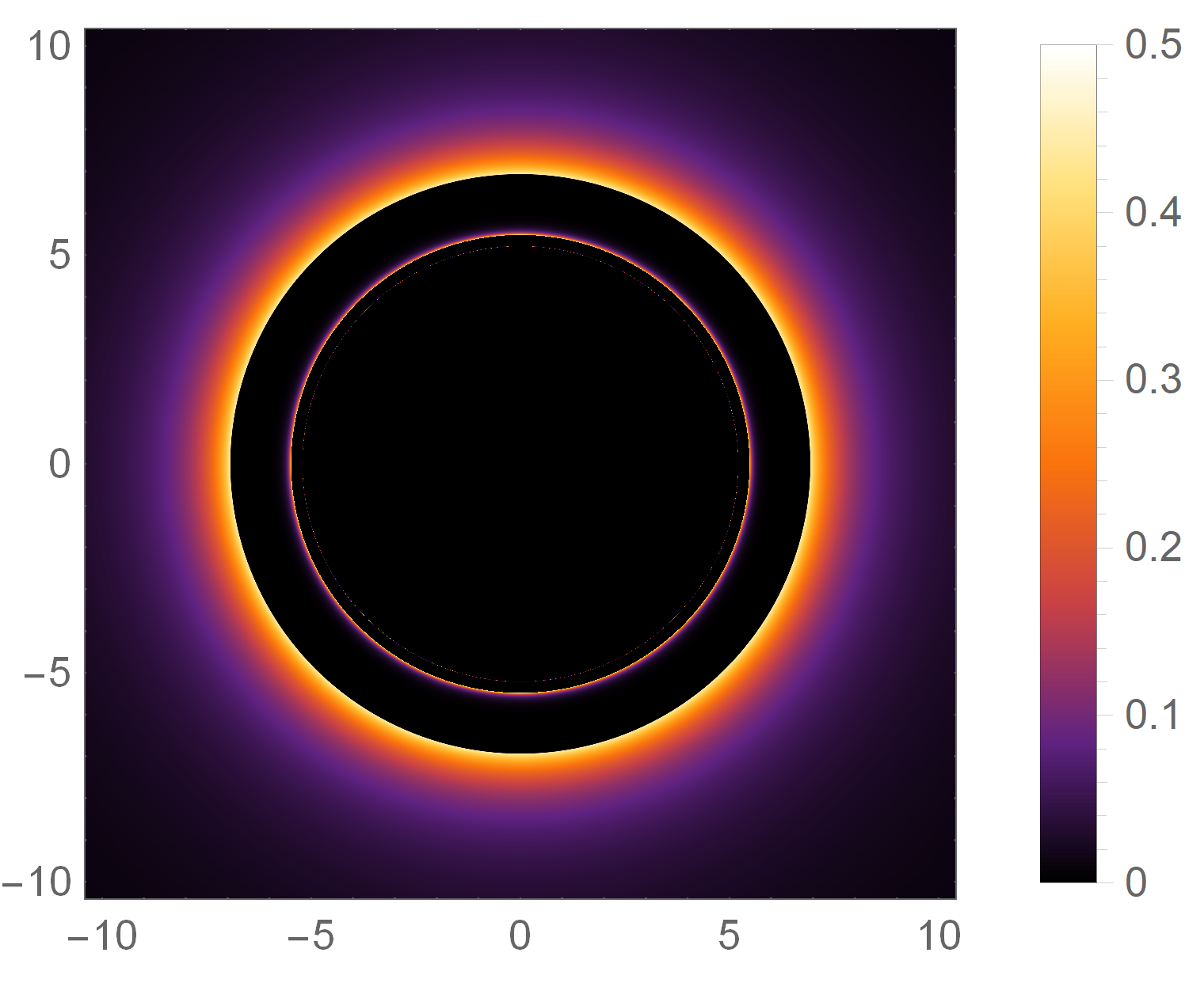
(b)   Schwarzschild

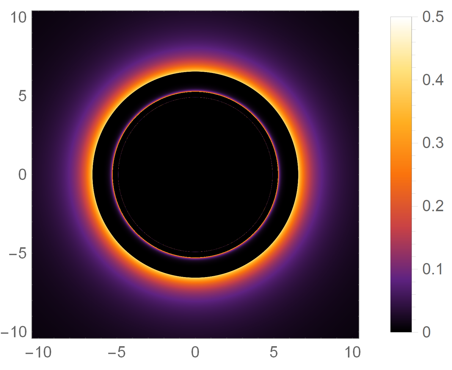
(c)   $\lambda/M=2.5$

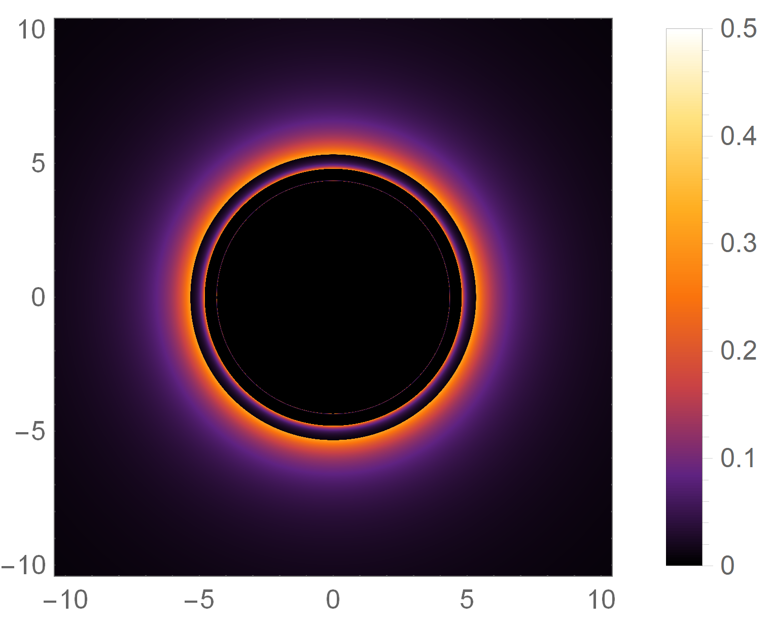
(d)   $\lambda/M=3.3$

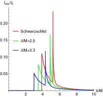
(e)   profile 2

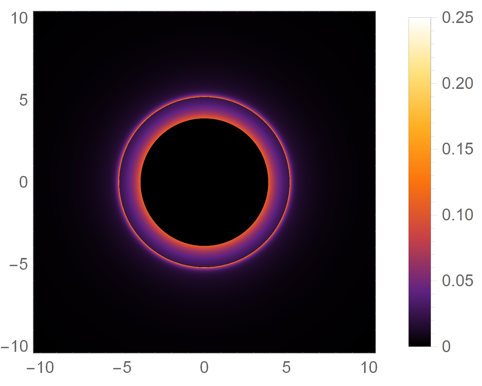
(f)   Schwarzschild

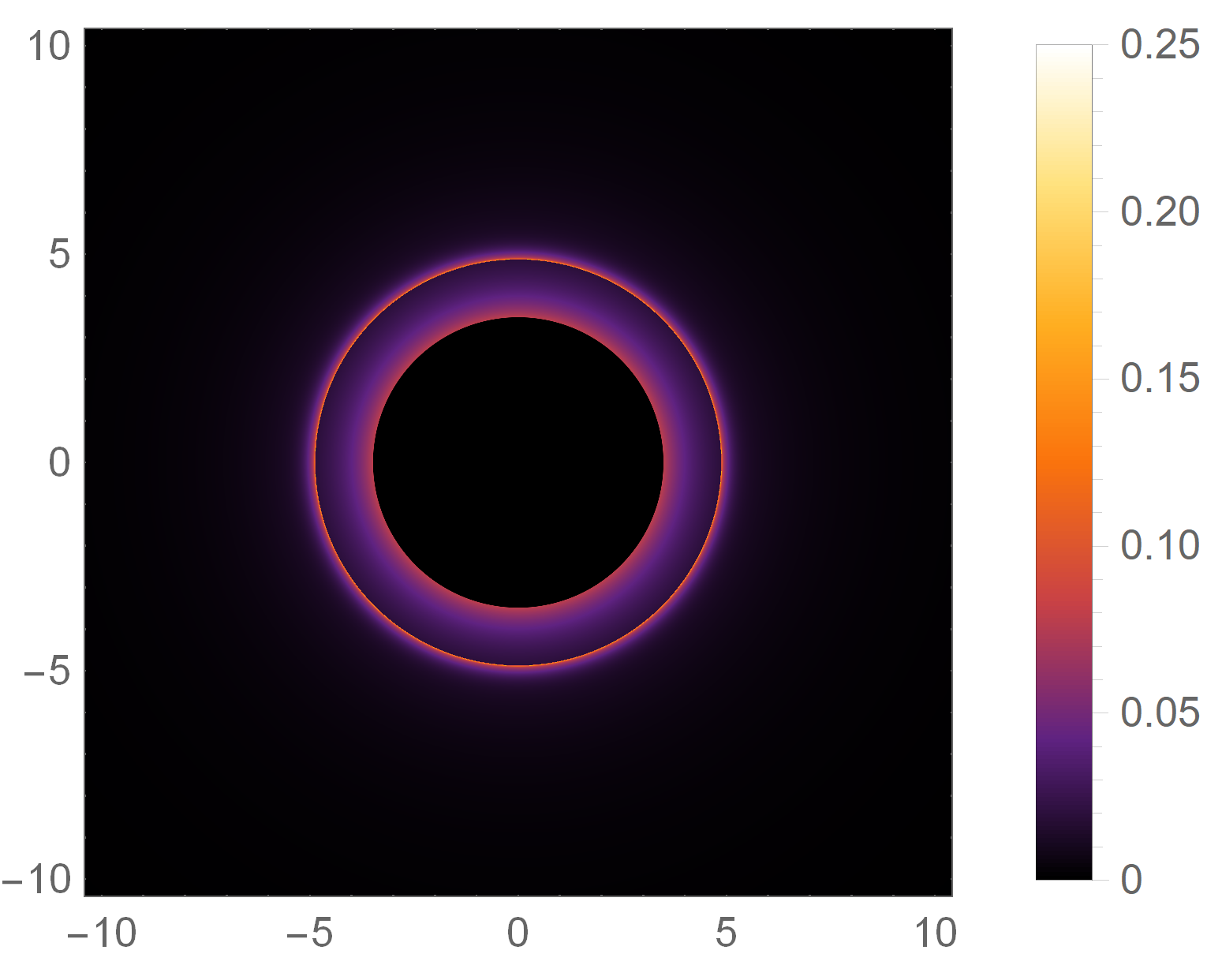
(g)   $\lambda/M=2.5$

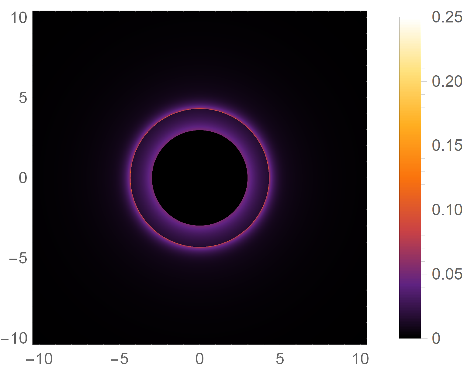
(h)   $\lambda/M=3.3$

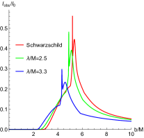
(i)   profile 3

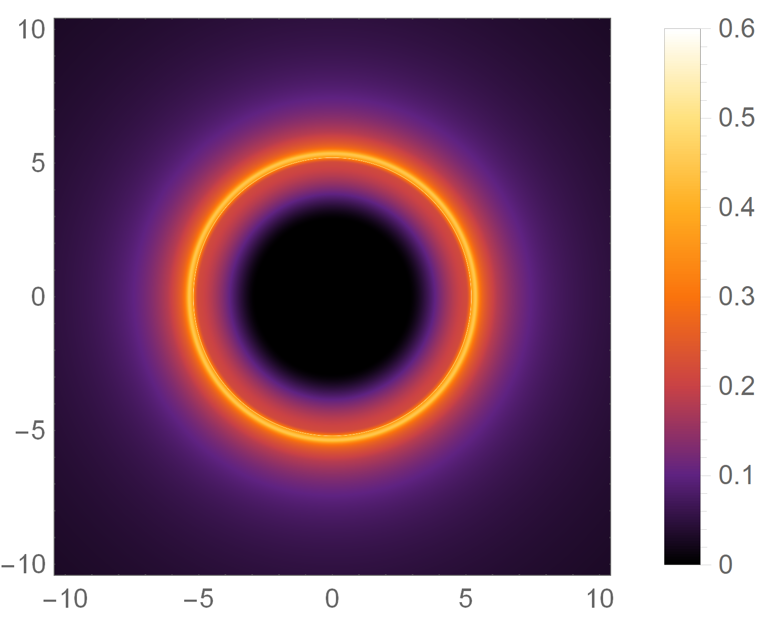
(j)   Schwarzschild

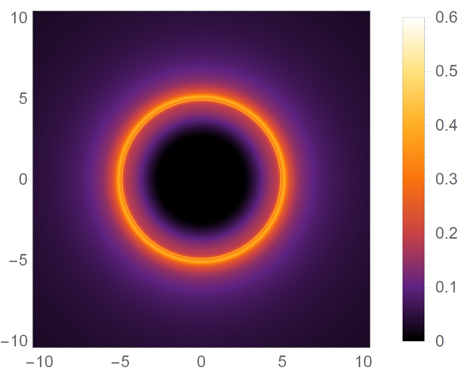
(k)   $\lambda/M=2.5$

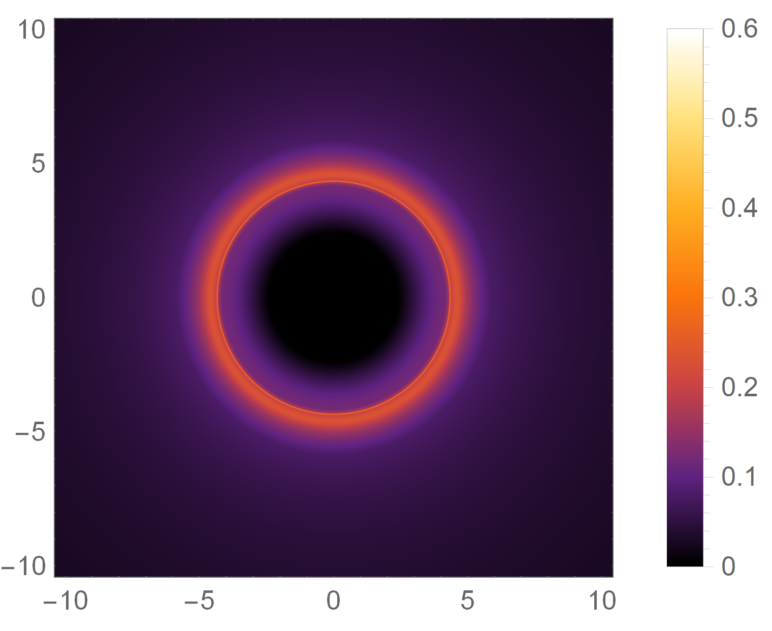
(l)   $\lambda/M=3.3$

Figure 9: The total observed intensities (figures (a), (e), (i)) and observational appearances (other figures) of the emission profile 1 (25), profile 2 (26) and profile 3 (27) of the thin accretion disks for Schwarzschild and scalarized Gauss-Bonnet black holes respectively.

V Rings and images of scalarized Gauss-Bonnet black hole illuminated by static spherical accretions

In the above section, we consider the accretion disk surrounding the black hole which is formed by the materials in the Universe that are trapped by a black hole and rotate with a large angular momentum. Another situation is when the angular momentum is extremely small, the materials will flow radially to the black hole and form the spherically symmetric accretion Yuan:2014gma . In this section, we will explore the images of scalarized black hole illuminated by the optically and geometrically thin static accretion with spherical symmetry. Here, the observed specific intensity $I(\nu_{o})$ seen by an observer at infinity $r=\infty$ (measured in erg s^-1 cm^-2 str^-1 Hz^-1) is obtained by the as follows Bambi:2013nla

$$I(\nu_{o})=\int_{\gamma}g^{3}j_{e}(\nu_{e})dl_{prop},$$ (28)

where $g=\nu_{o}/\nu_{e}=\sqrt{h(r)}$ is again the redshift factor Gan:2021pwu . $\nu_{o}$ and $\nu_{e}$ are the observed and emitted photon frequency, respectively. $j_{e}(\nu_{e})$ is the emissivity per unit volume in the rest frame and usually set $j(\nu_{e})\propto\delta(\nu_{r}-\nu_{e})/r^{2}$ where $\nu_{r}$ is rest-frame frequency of the emitter Bambi:2013nla . $dl_{prop}$ is the infinitesimal proper length read as

$$dl_{prop}=\sqrt{\frac{1}{f(r)}dr^{2}+r^{2}d\phi^{2}}=\sqrt{\frac{1}{f(r)}+r^{2}\left(\frac{d\phi}{dr}\right)^{2}}dr,$$ (29)

where $d\phi/dr$ is given by Eq.(18). So the formula Eq.(28) indicates that the integration is along the photon path $\gamma$. Further, by integrating Eq.(28) over the entire observed frequencies, we get the total observed intensity given by

$$I_{obs}=\int_{\nu_{o}}I(\nu_{o})d\nu_{o}=\int_{\nu_{e}}\int_{\gamma}g^{4}j_{e}(\nu_{e})dl_{prop}d\nu_{e}=\int_{\gamma}\frac{h(r)^{2}}{r^{2}}\sqrt{\frac{1}{f(r)}+r^{2}\left(\frac{d\phi}{dr}\right)^{2}}dr.$$ (30)

The total observed intensities and their corresponding images of scalarized black holes are shown in Fig.10. For the observed intensities, we find that there exists always a peak which is located at $b=b_{ph}$. With the increase of the coupling $\lambda$, the maximum value of the peak increases which means the maximum brightness of scalarized black hole is larger than that of Schwarzschild case. Moreover, the size of black hole shadow decreases as the coupling $\lambda$ increases, which was also shown in Fig.3(c). In the region inside shadow ($b<b_{ph}$), the observed intensity increases with $\lambda$. However in the region outside shadow ($b>b_{ph}$), it slightly decreases with $\lambda$. The observational appearances of scalarized black holes again confirm the above discussions.

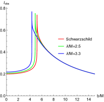
(a)   observed intensity

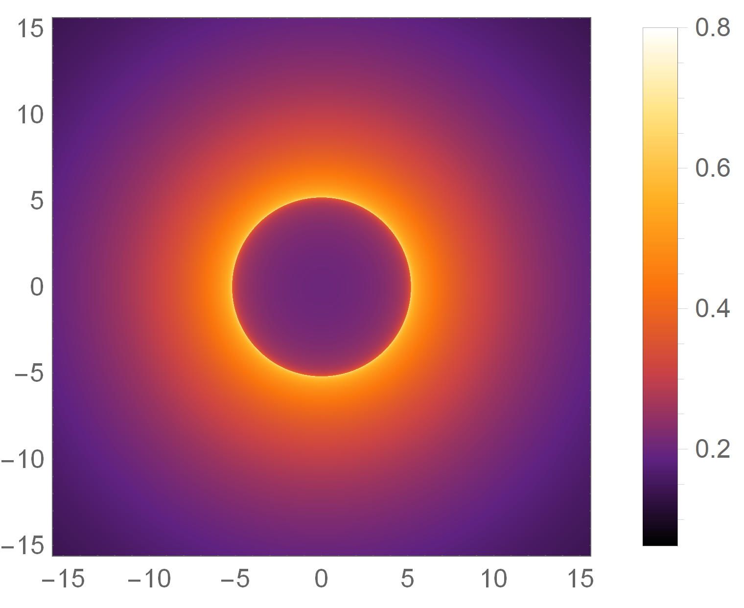
(b)   $\lambda/M=0$

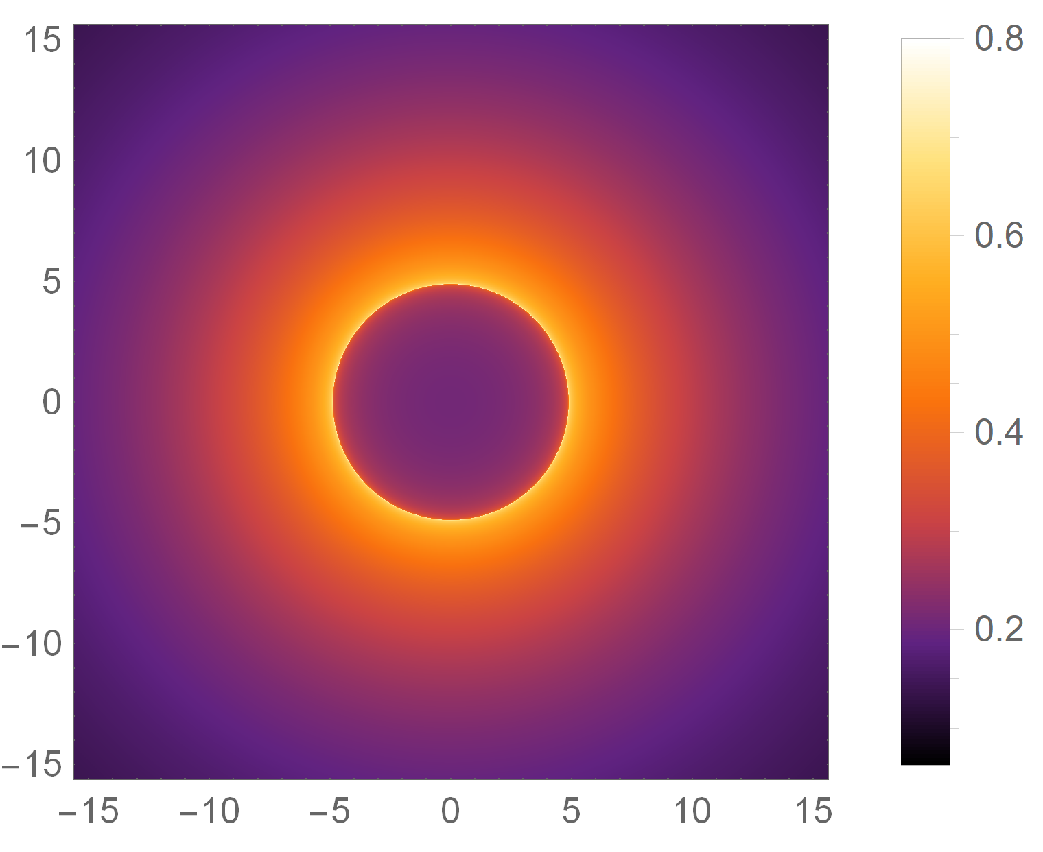
(c)   $\lambda/M=2.5$

(d)   $\lambda/M=3.3$

Figure 10: The total observed intensities (figure (a)) and observational appearances (other figures) of Schwarzschild and scalarized Gauss-Bonnet black holes surrounded by static spherical accretions, respectively.

VI Conclusion and discussion

EsGB theory, as one of the scalar-tensor theories, provides a theoretical framework that allows black hole with scalar hair. Specially, under certain conditions, there exist scalarized Gauss-Bonnet black hole solutions that are formed by spontaneous scalarization of the Schwarzschild black hole, which is induced by the curvature of the spacetime. The scalarized black hole solution and EsGB theory itself have been widely investigated from the theoretical and observational aspects. In this paper, we studied the optical features of the scalarized Gauss-Bonnet black hole illuminated by various static thin accretions in EsGB theory to explore the observational differences of black hole with and without spontaneous scalarization.

Firstly, we gave a short review on the Gauss-Bonnet black hole with spontaneous scalarization in EsGB theory. Concretely, we briefly illustrated the reason for forming spontaneous scalarization of Schwarzschild black hole and provided the background solutions of scalarized black hole for some selected coupling parameters $\lambda$. Then we computed event horizon, the radius of photon sphere, critical impact parameter and ISCO influenced by $\lambda$. The results showed that these physical quantities decreases as $\lambda$ increases, which implied the smaller size of black hole shadow. Further, by using the currently observable data of black hole shadows from EHT, we gave the upper limit for the coupling.

Secondly, we considered the scalarized black holes illuminated by the optically and geometrically thin accretion disks. Comparing to Schwarzschild case, the lensed and photon ring emissions from the accretion disk correspond to wider range of impact parameter for the scalarized black hole, and the demagnification factor in the second and third transfer functions are also suppressed. So the lensed and photon rings could be more easily to be observed. Then we considered three emission functions of accretion disks to compute the total observed intensities and images of scalarized black holes. For all models, we found that the scalarized black hole with larger coupling parameter $\lambda$ shows the smaller size of black hole shadow and weaker observed intensity but with the peak of larger width. Then we showed the scalarized black holes illuminated by the static spherical accretion. We found that a dark region indicated black hole shadow is surrounded by a bright photon ring. The shadow size for the scalarized black hole is smaller but the photon ring is more clear than that of Schwarzschild case.

In conclusion, we figured out the images of black holes with spontaneous scalarization illuminated by various static thin accretion disk and spherical accretion flow in EsGB theory. Compared to the black hole without spontaneous scalarization, our current results could disclose the significantly observational differences of black holes with spontaneous scalarization in EsGB theory. This preliminary study could provide a promising approach to test no-hair theorem by using black hole images. Here, we only consider the case of the finial state of scalarized black hole. So an interesting and meaningful direction is to investigate the image of black hole which is in the process of spontaneous scalarization. This will help us further understand the spontaneous scalarization of black hole and provide a potential method to test no-hair theorem from the observational perspective in the future.

- (1) LIGO Scientific, Virgo Collaboration, B. P. Abbott et al., “Observation of Gravitational Waves from a Binary Black Hole Merger,” Phys. Rev. Lett. 116 no. 6, (2016) 061102, arXiv:1602.03837 [gr-qc].
- (2) LIGO Scientific, Virgo Collaboration, B. P. Abbott et al., “GW170817: Observation of Gravitational Waves from a Binary Neutron Star Inspiral,” Phys. Rev. Lett. 119 no. 16, (2017) 161101, arXiv:1710.05832 [gr-qc].
- (3) LIGO Scientific, Virgo Collaboration, B. P. Abbott et al., “GW190425: Observation of a Compact Binary Coalescence with Total Mass ,” Astrophys. J. Lett. 892 no. 1, (2020) L3, arXiv:2001.01761 [astro-ph.HE].
- (4) Event Horizon Telescope Collaboration, K. Akiyama et al., “First M87 Event Horizon Telescope Results. I. The Shadow of the Supermassive Black Hole,” Astrophys. J. Lett. 875 (2019) L1, arXiv:1906.11238 [astro-ph.GA].
- (5) Event Horizon Telescope Collaboration, K. Akiyama et al., “First M87 Event Horizon Telescope Results. II. Array and Instrumentation,” Astrophys. J. Lett. 875 no. 1, (2019) L2, arXiv:1906.11239 [astro-ph.IM].
- (6) Event Horizon Telescope Collaboration, K. Akiyama et al., “First M87 Event Horizon Telescope Results. III. Data Processing and Calibration,” Astrophys. J. Lett. 875 no. 1, (2019) L3, arXiv:1906.11240 [astro-ph.GA].
- (7) Event Horizon Telescope Collaboration, K. Akiyama et al., “First M87 Event Horizon Telescope Results. IV. Imaging the Central Supermassive Black Hole,” Astrophys. J. Lett. 875 no. 1, (2019) L4, arXiv:1906.11241 [astro-ph.GA].
- (8) Event Horizon Telescope Collaboration, K. Akiyama et al., “First M87 Event Horizon Telescope Results. V. Physical Origin of the Asymmetric Ring,” Astrophys. J. Lett. 875 no. 1, (2019) L5, arXiv:1906.11242 [astro-ph.GA].
- (9) Event Horizon Telescope Collaboration, K. Akiyama et al., “First M87 Event Horizon Telescope Results. VI. The Shadow and Mass of the Central Black Hole,” Astrophys. J. Lett. 875 no. 1, (2019) L6, arXiv:1906.11243 [astro-ph.GA].
- (10) Event Horizon Telescope Collaboration, K. Akiyama et al., “First Sagittarius A* Event Horizon Telescope Results. I. The Shadow of the Supermassive Black Hole in the Center of the Milky Way,” Astrophys. J. Lett. 930 no. 2, (2022) L12.
- (11) Event Horizon Telescope Collaboration, K. Akiyama et al., “First Sagittarius A* Event Horizon Telescope Results. II. EHT and Multiwavelength Observations, Data Processing, and Calibration,” Astrophys. J. Lett. 930 no. 2, (2022) L13.
- (12) Event Horizon Telescope Collaboration, K. Akiyama et al., “First Sagittarius A* Event Horizon Telescope Results. III. Imaging of the Galactic Center Supermassive Black Hole,” Astrophys. J. Lett. 930 no. 2, (2022) L14.
- (13) Event Horizon Telescope Collaboration, K. Akiyama et al., “First Sagittarius A* Event Horizon Telescope Results. IV. Variability, Morphology, and Black Hole Mass,” Astrophys. J. Lett. 930 no. 2, (2022) L15.
- (14) Event Horizon Telescope Collaboration, K. Akiyama et al., “First Sagittarius A* Event Horizon Telescope Results. V. Testing Astrophysical Models of the Galactic Center Black Hole,” Astrophys. J. Lett. 930 no. 2, (2022) L16.
- (15) Event Horizon Telescope Collaboration, K. Akiyama et al., “First Sagittarius A* Event Horizon Telescope Results. VI. Testing the Black Hole Metric,” Astrophys. J. Lett. 930 no. 2, (2022) L17.
- (16) K. S. Stelle, “Renormalization of Higher Derivative Quantum Gravity,” Phys. Rev. D 16 (1977) 953–969.
- (17) G. W. Horndeski, “Second-order scalar-tensor field equations in a four-dimensional space,” Int. J. Theor. Phys. 10 (1974) 363–384.
- (18) C. Deffayet, S. Deser, and G. Esposito-Farese, “Generalized Galileons: All scalar models whose curved background extensions maintain second-order field equations and stress-tensors,” Phys. Rev. D 80 (2009) 064015, arXiv:0906.1967 [gr-qc].
- (19) S. Mignemi and N. R. Stewart, “Charged black holes in effective string theory,” Phys. Rev. D 47 (1993) 5259–5269, arXiv:hep-th/9212146.
- (20) P. Kanti, N. E. Mavromatos, J. Rizos, K. Tamvakis, and E. Winstanley, “Dilatonic black holes in higher curvature string gravity,” Phys. Rev. D 54 (1996) 5049–5058, arXiv:hep-th/9511071.
- (21) T. Torii, H. Yajima, and K.-i. Maeda, “Dilatonic black holes with Gauss-Bonnet term,” Phys. Rev. D 55 (1997) 739–753, arXiv:gr-qc/9606034.
- (22) B. Kleihaus, J. Kunz, and E. Radu, “Rotating Black Holes in Dilatonic Einstein-Gauss-Bonnet Theory,” Phys. Rev. Lett. 106 (2011) 151104, arXiv:1101.2868 [gr-qc].
- (23) T. P. Sotiriou and S.-Y. Zhou, “Black hole hair in generalized scalar-tensor gravity,” Phys. Rev. Lett. 112 (2014) 251102, arXiv:1312.3622 [gr-qc].
- (24) D. Ayzenberg and N. Yunes, “Slowly-Rotating Black Holes in Einstein-Dilaton-Gauss-Bonnet Gravity: Quadratic Order in Spin Solutions,” Phys. Rev. D 90 (2014) 044066, arXiv:1405.2133 [gr-qc]. [Erratum: Phys.Rev.D 91, 069905 (2015)].
- (25) B. Kleihaus, J. Kunz, S. Mojica, and M. Zagermann, “Rapidly Rotating Neutron Stars in Dilatonic Einstein-Gauss-Bonnet Theory,” Phys. Rev. D 93 no. 6, (2016) 064077, arXiv:1601.05583 [gr-qc].
- (26) J. D. Bekenstein, “Transcendence of the law of baryon-number conservation in black hole physics,” Phys. Rev. Lett. 28 (1972) 452–455.
- (27) C. Teitelboim, “Nonmeasurability of the lepton number of a black hole,” Lett. Nuovo Cim. 3S2 (1972) 397–400.
- (28) D. D. Doneva and S. S. Yazadjiev, “New Gauss-Bonnet Black Holes with Curvature-Induced Scalarization in Extended Scalar-Tensor Theories,” Phys. Rev. Lett. 120 no. 13, (2018) 131103, arXiv:1711.01187 [gr-qc].
- (29) H. O. Silva, J. Sakstein, L. Gualtieri, T. P. Sotiriou, and E. Berti, “Spontaneous scalarization of black holes and compact stars from a Gauss-Bonnet coupling,” Phys. Rev. Lett. 120 no. 13, (2018) 131104, arXiv:1711.02080 [gr-qc].
- (30) G. Antoniou, A. Bakopoulos, and P. Kanti, “Evasion of No-Hair Theorems and Novel Black-Hole Solutions in Gauss-Bonnet Theories,” Phys. Rev. Lett. 120 no. 13, (2018) 131102, arXiv:1711.03390 [hep-th].
- (31) T. Damour and G. Esposito-Farese, “Nonperturbative strong field effects in tensor - scalar theories of gravitation,” Phys. Rev. Lett. 70 (1993) 2220–2223.
- (32) D. D. Doneva and S. S. Yazadjiev, “Neutron star solutions with curvature induced scalarization in the extended Gauss-Bonnet scalar-tensor theories,” JCAP 04 (2018) 011, arXiv:1712.03715 [gr-qc].
- (33) G. Antoniou, A. Bakopoulos, P. Kanti, B. Kleihaus, and J. Kunz, “Novel Einstein–scalar-Gauss-Bonnet wormholes without exotic matter,” Phys. Rev. D 101 no. 2, (2020) 024033, arXiv:1904.13091 [hep-th].
- (34) R. Ibadov, B. Kleihaus, J. Kunz, and S. Murodov, “Wormholes in Einstein-scalar-Gauss-Bonnet theories with a scalar self-interaction potential,” Phys. Rev. D 102 no. 6, (2020) 064010, arXiv:2006.13008 [gr-qc].
- (35) J. L. Blázquez-Salcedo, D. D. Doneva, S. Kahlen, J. Kunz, P. Nedkova, and S. S. Yazadjiev, “Axial perturbations of the scalarized Einstein-Gauss-Bonnet black holes,” Phys. Rev. D 101 no. 10, (2020) 104006, arXiv:2003.02862 [gr-qc].
- (36) J. L. Blázquez-Salcedo, D. D. Doneva, S. Kahlen, J. Kunz, P. Nedkova, and S. S. Yazadjiev, “Polar quasinormal modes of the scalarized Einstein-Gauss-Bonnet black holes,” Phys. Rev. D 102 no. 2, (2020) 024086, arXiv:2006.06006 [gr-qc].
- (37) J. L. Blázquez-Salcedo, D. D. Doneva, J. Kunz, and S. S. Yazadjiev, “Radial perturbations of the scalarized Einstein-Gauss-Bonnet black holes,” Phys. Rev. D 98 no. 8, (2018) 084011, arXiv:1805.05755 [gr-qc].
- (38) C. A. R. Herdeiro and E. Radu, “Black hole scalarization from the breakdown of scale invariance,” Phys. Rev. D 99 no. 8, (2019) 084039, arXiv:1901.02953 [gr-qc].
- (39) C. A. R. Herdeiro, E. Radu, N. Sanchis-Gual, and J. A. Font, “Spontaneous Scalarization of Charged Black Holes,” Phys. Rev. Lett. 121 no. 10, (2018) 101102, arXiv:1806.05190 [gr-qc].
- (40) P. G. S. Fernandes, C. A. R. Herdeiro, A. M. Pombo, E. Radu, and N. Sanchis-Gual, “Spontaneous Scalarisation of Charged Black Holes: Coupling Dependence and Dynamical Features,” Class. Quant. Grav. 36 no. 13, (2019) 134002, arXiv:1902.05079 [gr-qc]. [Erratum: Class.Quant.Grav. 37, 049501 (2020)].
- (41) Y. Brihaye, C. Herdeiro, and E. Radu, “The scalarised Schwarzschild-NUT spacetime,” Phys. Lett. B 788 (2019) 295–301, arXiv:1810.09560 [gr-qc].
- (42) A. Bakopoulos, G. Antoniou, and P. Kanti, “Novel Black-Hole Solutions in Einstein-Scalar-Gauss-Bonnet Theories with a Cosmological Constant,” Phys. Rev. D 99 no. 6, (2019) 064003, arXiv:1812.06941 [hep-th].
- (43) Y. Brihaye, C. Herdeiro, and E. Radu, “Black Hole Spontaneous Scalarisation with a Positive Cosmological Constant,” Phys. Lett. B 802 (2020) 135269, arXiv:1910.05286 [gr-qc].
- (44) A. Bakopoulos, P. Kanti, and N. Pappas, “Existence of solutions with a horizon in pure scalar-Gauss-Bonnet theories,” Phys. Rev. D 101 no. 4, (2020) 044026, arXiv:1910.14637 [hep-th].
- (45) A. Bakopoulos, P. Kanti, and N. Pappas, “Large and ultracompact Gauss-Bonnet black holes with a self-interacting scalar field,” Phys. Rev. D 101 no. 8, (2020) 084059, arXiv:2003.02473 [hep-th].
- (46) K. Lin, S. Zhang, C. Zhang, X. Zhao, B. Wang, and A. Wang, “No static regular black holes in Einstein-complex-scalar-Gauss-Bonnet gravity,” Phys. Rev. D 102 no. 2, (2020) 024034, arXiv:2004.04773 [gr-qc].
- (47) H. Guo, S. Kiorpelidi, X.-M. Kuang, E. Papantonopoulos, B. Wang, and J.-P. Wu, “Spontaneous holographic scalarization of black holes in Einstein-scalar-Gauss-Bonnet theories,” Phys. Rev. D 102 no. 8, (2020) 084029, arXiv:2006.10659 [hep-th].
- (48) H. Guo, W.-L. Qian, and B. Wang, “Phase structure of holographic superconductors in an Einstein-scalar-Gauss-Bonnet theory with spontaneous scalarization,” Phys. Rev. D 109 no. 12, (2024) 124038, arXiv:2401.09846 [gr-qc].
- (49) H. Guo, X.-M. Kuang, E. Papantonopoulos, and B. Wang, “Horizon curvature and spacetime structure influences on black hole scalarization,” Eur. Phys. J. C 81 no. 9, (2021) 842, arXiv:2012.11844 [gr-qc].
- (50) L. G. Collodel, B. Kleihaus, J. Kunz, and E. Berti, “Spinning and excited black holes in Einstein-scalar-Gauss–Bonnet theory,” Class. Quant. Grav. 37 no. 7, (2020) 075018, arXiv:1912.05382 [gr-qc].
- (51) A. Dima, E. Barausse, N. Franchini, and T. P. Sotiriou, “Spin-induced black hole spontaneous scalarization,” Phys. Rev. Lett. 125 no. 23, (2020) 231101, arXiv:2006.03095 [gr-qc].
- (52) D. D. Doneva, L. G. Collodel, C. J. Krüger, and S. S. Yazadjiev, “Spin-induced scalarization of Kerr black holes with a massive scalar field,” Eur. Phys. J. C 80 no. 12, (2020) 1205, arXiv:2009.03774 [gr-qc].
- (53) C. A. R. Herdeiro, E. Radu, H. O. Silva, T. P. Sotiriou, and N. Yunes, “Spin-induced scalarized black holes,” Phys. Rev. Lett. 126 no. 1, (2021) 011103, arXiv:2009.03904 [gr-qc].
- (54) E. Berti, L. G. Collodel, B. Kleihaus, and J. Kunz, “Spin-induced black-hole scalarization in Einstein-scalar-Gauss-Bonnet theory,” Phys. Rev. Lett. 126 no. 1, (2021) 011104, arXiv:2009.03905 [gr-qc].
- (55) G. Lara, H. P. Pfeiffer, N. A. Wittek, N. L. Vu, K. C. Nelli, A. Carpenter, G. Lovelace, M. A. Scheel, and W. Throwe, “Scalarization of isolated black holes in scalar Gauss-Bonnet theory in the fixing-the-equations approach,” Phys. Rev. D 110 no. 2, (2024) 024033, arXiv:2403.08705 [gr-qc].
- (56) Y. Liu, C.-Y. Zhang, Q. Chen, Z. Cao, Y. Tian, and B. Wang, “Critical scalarization and descalarization of black holes in a generalized scalar-tensor theory,” Sci. China Phys. Mech. Astron. 66 no. 10, (2023) 100412, arXiv:2208.07548 [gr-qc].
- (57) L. K. Wong, C. A. R. Herdeiro, and E. Radu, “Constraining spontaneous black hole scalarization in scalar-tensor-Gauss-Bonnet theories with current gravitational-wave data,” Phys. Rev. D 106 no. 2, (2022) 024008, arXiv:2204.09038 [gr-qc].
- (58) J. L. Synge, “The Escape of Photons from Gravitationally Intense Stars,” Mon. Not. Roy. Astron. Soc. 131 no. 3, (1966) 463–466.
- (59) J. M. Bardeen, “Timelike and null geodesics in the Kerr metric,” Proceedings, Ecole d’Eté de Physique Théorique: Les Astres Occlus : Les Houches, France, August, 1972, 215-240 (1973) 215–240.
- (60) L. Amarilla, E. F. Eiroa, and G. Giribet, “Null geodesics and shadow of a rotating black hole in extended Chern-Simons modified gravity,” Phys. Rev. D 81 (2010) 124045, arXiv:1005.0607 [gr-qc].
- (61) S.-W. Wei and Y.-X. Liu, “Observing the shadow of Einstein-Maxwell-Dilaton-Axion black hole,” JCAP 11 (2013) 063, arXiv:1311.4251 [gr-qc].
- (62) M. Wang, S. Chen, and J. Jing, “Shadow casted by a Konoplya-Zhidenko rotating non-Kerr black hole,” JCAP 10 (2017) 051, arXiv:1707.09451 [gr-qc].
- (63) S. Dastan, R. Saffari, and S. Soroushfar, “Shadow of a charged rotating black hole in f(R) gravity,” Eur. Phys. J. Plus 137 no. 9, (2022) 1002, arXiv:1606.06994 [gr-qc].
- (64) H.-M. Wang, Y.-M. Xu, and S.-W. Wei, “Shadows of Kerr-like black holes in a modified gravity theory,” JCAP 03 (2019) 046, arXiv:1810.12767 [gr-qc].
- (65) X.-M. Kuang, Z.-Y. Tang, B. Wang, and A. Wang, “Constraining a modified gravity theory in strong gravitational lensing and black hole shadow observations,” Phys. Rev. D 106 no. 6, (2022) 064012, arXiv:2206.05878 [gr-qc].
- (66) Y. Meng, X.-M. Kuang, X.-J. Wang, and J.-P. Wu, “Shadow revisiting and weak gravitational lensing with Chern-Simons modification,” Phys. Lett. B 841 (2023) 137940, arXiv:2305.04210 [gr-qc].
- (67) Y. Meng, X.-M. Kuang, and Z.-Y. Tang, “Photon regions, shadow observables, and constraints from M87* of a charged rotating black hole,” Phys. Rev. D 106 no. 6, (2022) 064006, arXiv:2204.00897 [gr-qc].
- (68) A. Addazi, S. Capozziello, and S. Odintsov, “Chaotic solutions and black hole shadow in gravity,” Phys. Lett. B 816 (2021) 136257, arXiv:2103.16856 [gr-qc].
- (69) P.-C. Li, M. Guo, and B. Chen, “Shadow of a Spinning Black Hole in an Expanding Universe,” Phys. Rev. D 101 no. 8, (2020) 084041, arXiv:2001.04231 [gr-qc].
- (70) X.-M. Kuang and A. Övgün, “Strong gravitational lensing and shadow constraint from M87* of slowly rotating Kerr-like black hole,” Annals Phys. 447 (2022) 169147, arXiv:2205.11003 [gr-qc].
- (71) R. Kumar, S. G. Ghosh, and A. Wang, “Shadow cast and deflection of light by charged rotating regular black holes,” Phys. Rev. D 100 no. 12, (2019) 124024, arXiv:1912.05154 [gr-qc].
- (72) R. Shaikh, K. Pal, K. Pal, and T. Sarkar, “Constraining alternatives to the Kerr black hole,” Mon. Not. Roy. Astron. Soc. 506 no. 1, (2021) 1229–1236, arXiv:2102.04299 [gr-qc].
- (73) S. Vagnozzi et al., “Horizon-scale tests of gravity theories and fundamental physics from the Event Horizon Telescope image of Sagittarius A,” Class. Quant. Grav. 40 no. 16, (2023) 165007, arXiv:2205.07787 [gr-qc].
- (74) T.-T. Sui, Q.-M. Fu, and W.-D. Guo, “The shadows of accelerating Kerr-Newman black hole and constraints from M87*,” Phys. Lett. B 845 (2023) 138135, arXiv:2311.10930 [gr-qc].
- (75) X.-M. Kuang, Y. Meng, E. Papantonopoulos, and X.-J. Wang, “Using the shadow of a black hole to examine the energy exchange between axion matter and a rotating black hole,” Phys. Rev. D 110 no. 6, (2024) L061503, arXiv:2406.11932 [gr-qc].
- (76) Event Horizon Telescope Collaboration, O. Porth et al., “The Event Horizon General Relativistic Magnetohydrodynamic Code Comparison Project,” Astrophys. J. Suppl. 243 no. 2, (2019) 26, arXiv:1904.04923 [astro-ph.HE].
- (77) S. E. Gralla, D. E. Holz, and R. M. Wald, “Black Hole Shadows, Photon Rings, and Lensing Rings,” Phys. Rev. D 100 no. 2, (2019) 024018, arXiv:1906.00873 [astro-ph.HE].
- (78) H. Falcke, F. Melia, and E. Agol, “Viewing the shadow of the black hole at the galactic center,” Astrophys. J. Lett. 528 (2000) L13, arXiv:astro-ph/9912263.
- (79) R. Narayan, M. D. Johnson, and C. F. Gammie, “The Shadow of a Spherically Accreting Black Hole,” Astrophys. J. Lett. 885 no. 2, (2019) L33, arXiv:1910.02957 [astro-ph.HE].
- (80) M. D. Johnson et al., “Universal interferometric signatures of a black hole’s photon ring,” Sci. Adv. 6 no. 12, (2020) eaaz1310, arXiv:1907.04329 [astro-ph.IM].
- (81) X.-X. Zeng, H.-Q. Zhang, and H. Zhang, “Shadows and photon spheres with spherical accretions in the four-dimensional Gauss–Bonnet black hole,” Eur. Phys. J. C 80 no. 9, (2020) 872, arXiv:2004.12074 [gr-qc].
- (82) X.-X. Zeng and H.-Q. Zhang, “Influence of quintessence dark energy on the shadow of black hole,” Eur. Phys. J. C 80 no. 11, (2020) 1058, arXiv:2007.06333 [gr-qc].
- (83) J. Peng, M. Guo, and X.-H. Feng, “Influence of quantum correction on black hole shadows, photon rings, and lensing rings,” Chin. Phys. C 45 no. 8, (2021) 085103, arXiv:2008.00657 [gr-qc].
- (84) X. Qin, S. Chen, and J. Jing, “Image of a regular phantom compact object and its luminosity under spherical accretions,” Class. Quant. Grav. 38 no. 11, (2021) 115008, arXiv:2011.04310 [gr-qc].
- (85) L. Chakhchi, H. El Moumni, and K. Masmar, “Shadows and optical appearance of a power-Yang-Mills black hole surrounded by different accretion disk profiles,” Phys. Rev. D 105 no. 6, (2022) 064031.
- (86) S. Guo, G.-R. Li, and E.-W. Liang, “Influence of accretion flow and magnetic charge on the observed shadows and rings of the Hayward black hole,” Phys. Rev. D 105 no. 2, (2022) 023024, arXiv:2112.11227 [astro-ph.HE].
- (87) S. Hu, C. Deng, D. Li, X. Wu, and E. Liang, “Observational signatures of Schwarzschild-MOG black holes in scalar-tensor-vector gravity: shadows and rings with different accretions,” Eur. Phys. J. C 82 no. 10, (2022) 885.
- (88) S. Wen, W. Hong, and J. Tao, “Observational Appearances of Magnetically Charged Black Holes in Born-Infeld Electrodynamics,” Eur. Phys. J. C 83 (2023) 277, arXiv:2212.03021 [gr-qc].
- (89) Y. Meng, X.-M. Kuang, X.-J. Wang, B. Wang, and J.-P. Wu, “Images of hairy Reissner–Nordström black hole illuminated by static accretions,” Eur. Phys. J. C 84 no. 3, (2024) 305, arXiv:2401.05634 [gr-qc].
- (90) X.-J. Gao, T.-T. Sui, X.-X. Zeng, Y.-S. An, and Y.-P. Hu, “Investigating shadow images and rings of the charged Horndeski black hole illuminated by various thin accretions,” Eur. Phys. J. C 83 (2023) 1052, arXiv:2311.11780 [gr-qc].
- (91) X.-J. Wang, X.-M. Kuang, Y. Meng, B. Wang, and J.-P. Wu, “Rings and images of Horndeski hairy black hole illuminated by various thin accretions,” Phys. Rev. D 107 no. 12, (2023) 124052, arXiv:2304.10015 [gr-qc].
- (92) Y. Chen, P. Wang, and H. Yang, “Interferometric signatures of black holes with multiple photon spheres,” Phys. Rev. D 110 no. 4, (2024) 044020, arXiv:2312.10304 [gr-qc].
- (93) X. Yang, M. Tang, and Z. Xu, “Exploring the possibility of testing the no-hair theorem with Minkowski-deformed regular hairy black holes via photon rings,” Eur. Phys. J. C 84 no. 9, (2024) 977, arXiv:2408.12318 [gr-qc].
- (94) H. Lu, A. Perkins, C. N. Pope, and K. S. Stelle, “Black Holes in Higher-Derivative Gravity,” Phys. Rev. Lett. 114 no. 17, (2015) 171601, arXiv:1502.01028 [hep-th].
- (95) X.-J. Wang, G. Fu, P. Liu, X.-M. Kuang, B. Wang, and J.-P. Wu, “Black holes with scalar hair: Extending from and beyond the Schwarzschild solution,” Phys. Rev. D 108 no. 12, (2023) 124077, arXiv:2307.13440 [gr-qc].
- (96) Y. S. Myung, “Two instabilities of Schwarzschild-AdS black holes in Einstein–Weyl-scalar theory,” Eur. Phys. J. C 83 no. 10, (2023) 902, arXiv:2307.14625 [gr-qc].
- (97) V. Cardoso, I. P. Carucci, P. Pani, and T. P. Sotiriou, “Black holes with surrounding matter in scalar-tensor theories,” Phys. Rev. Lett. 111 (2013) 111101, arXiv:1308.6587 [gr-qc].
- (98) V. Cardoso, I. P. Carucci, P. Pani, and T. P. Sotiriou, “Matter around Kerr black holes in scalar-tensor theories: scalarization and superradiant instability,” Phys. Rev. D 88 (2013) 044056, arXiv:1305.6936 [gr-qc].
- (99) Q. Gan, P. Wang, H. Wu, and H. Yang, “Photon spheres and spherical accretion image of a hairy black hole,” Phys. Rev. D 104 no. 2, (2021) 024003, arXiv:2104.08703 [gr-qc].
- (100) Q. Gan, P. Wang, H. Wu, and H. Yang, “Photon ring and observational appearance of a hairy black hole,” Phys. Rev. D 104 no. 4, (2021) 044049, arXiv:2105.11770 [gr-qc].
- (101) Y. Meng, X.-M. Kuang, X.-J. Wang, B. Wang, and J.-P. Wu, “Images from disk and spherical accretions of hairy Schwarzschild black holes,” Phys. Rev. D 108 no. 6, (2023) 064013, arXiv:2306.10459 [gr-qc].
- (102) R. Kumar and S. G. Ghosh, “Rotating black holes in Einstein-Gauss-Bonnet gravity and its shadow,” JCAP 07 (2020) 053, arXiv:2003.08927 [gr-qc].
- (103) Event Horizon Telescope Collaboration, P. Kocherlakota et al., “Constraints on black-hole charges with the 2017 EHT observations of M87*,” Phys. Rev. D 103 no. 10, (2021) 104047, arXiv:2105.09343 [gr-qc].
- (104) M. Wielgus, “Photon rings of spherically symmetric black holes and robust tests of non-Kerr metrics,” Phys. Rev. D 104 no. 12, (2021) 124058, arXiv:2109.10840 [gr-qc].
- (105) G. S. Bisnovatyi-Kogan and O. Y. Tsupko, “Analytical study of higher-order ring images of the accretion disk around a black hole,” Phys. Rev. D 105 no. 6, (2022) 064040, arXiv:2201.01716 [gr-qc].
- (106) H.-M. Wang, Z.-C. Lin, and S.-W. Wei, “Optical appearance of Einstein-Æther black hole surrounded by thin disk,” Nucl. Phys. B 985 (2022) 116026, arXiv:2205.13174 [gr-qc].
- (107) J. Yang, C. Zhang, and Y. Ma, “Shadow and stability of quantum-corrected black holes,” Eur. Phys. J. C 83 no. 7, (2023) 619, arXiv:2211.04263 [gr-qc].
- (108) F. Yuan and R. Narayan, “Hot Accretion Flows Around Black Holes,” Ann. Rev. Astron. Astrophys. 52 (2014) 529–588, arXiv:1401.0586 [astro-ph.HE].
- (109) C. Bambi, “Can the supermassive objects at the centers of galaxies be traversable wormholes? The first test of strong gravity for mm/sub-mm very long baseline interferometry facilities,” Phys. Rev. D 87 (2013) 107501, arXiv:1304.5691 [gr-qc].