Positive definiteness constraints of effective scalar potential in Georgi-Machacek Model

Abstract

Georgi-Machacek (GM) Model, which extends the Higgs sector of standard model with additional triplets, can preserve the custodial symmetry at tree level and allow large triplet vacuum expectation values of order $\cal{O}$(10) GeV. Various theoretical constraints can be imposed on the parameters of the Lagrangian, including the bounded-from-below constraints for the tree-level scalar potential. We propose to go beyond the tree-level bounded-from-below constraints and discuss the positive definiteness constraints for the effective potential of GM model to ensure the non-existence of a deeper vacuum in large field value regions. Based on one-loop renormalization group-improved (RG-improved) effective potential and new positive definite criteria for homogeneous polynomial with multiple variables (which is necessary because of the custodial symmetry breaking effects by loops), we can analyse numerically the positive definiteness constraints for GM model. Our numerical results indicate that the ranges of the quartic couplings allowed by the positive definiteness requirements are quite different from that derived from the tree-level bounded-from-below requirements. Especially, some parameter regions excluded previously by the tree-level bounded-from-below requirements can still satisfy the positive definite requirements with the one-loop RG-improved scalar potential. Besides, a portion of parameter space that can satisfy the tree-level bounded-from-below constraints with EW scale coupling inputs, should in fact be ruled out by the the positive definiteness requirements of the effective potential at large field value regions.

1 Introduction

The Standard Model (SM) of particle physics have been tested by a vast number of experiments and can be regard as a successful low energy effective theory at or below the electroweak (EW) scale. Especially, the discovery of the 125 GeV Higgs particle by the collaborative efforts of the ATLAS and CMS ATLAS:higgs ; CMS:higgs at the Large Hadron Collider (LHC) fills the last missing piece of SM. Although the Higgs boson discovered by LHC is quite consistent with the prediction of the SM, the scalar sector responsible for the electroweak symmetry breaking (EWSB) can still be quite different from the simple scalar sector of the SM. In fact, the possibility of an extended Higgs sector is still consistent with current experimental bounds, predicting additional scalars other than the 125 GeV scalar. Searching for such new scalars and finding out the origin of EWSB are the most important tasks of LHC.

Extending the SM with additional scalars can be well-motivated theoretically. For example, the Georgi-Machacek (GM) model GM ; GM2 ; GM3 ; GM4 ; GM5 ; GM6 ; GM7 ; GM8 ; GM9 ; GM10 ; GM11 ; GM12 ; GM13 ; GM14 ; GM15 ; GM16 ; GM17 ; GM18 ; GM19 ; GM20 ; GM21 ; GM22 ; GM23 ; GM24 ; GM25 ; GM26 ; GM27 ; GM28 ; GM29 ; GM30 ; GM31 ; GM32 ; GM33 ; GM34 ; GM35 ; GM36 ; GM37 ; GM38 ; GM39 ; GM40 ; GM41 ; GM63 ; GM42 ; GM43 ; GM44 ; GM45 ; GM46 ; GM47 ; GM48 ; GM49 ; GM50 ; GM51 ; GM52 ; GM53 ; GM54 ; GM55 ; GM56 ; GM57 ; GM58 ; GM59 ; GM60 ; GM61 ; GM62 ; GM64 , which adds to the SM an additional complex $SU(2)_{L}$ triplet scalar $\chi$ with unit hypercharge and a real $SU(2)_{L}$ triplet scalar $\xi$ with zero hypercharge, can preserve non-trivially the custodial symmetry at tree level with alignment Vacuum Expectation Values (VEVs) between the complex and real triplets after EWSB, rendering possible large triplet VEVs of order $\cal{O}$(10)GeV. With the triplet scalar $\chi$, the Type-II neutrino seesaw mechanism GM28 ; GM48 can be naturally accommodated in GM model to explain the tiny neutrino masses, although the embedding of other neutrino generation mechanisms can also be possible GM15 . GM model can also account for the baryon asymmetry of the universe (BAU) via electroweak baryogenesis, resulting in the emitting of detectable gravitational wave (GW) during electroweak phase transition (EWPT) GM52 ; GM53 ; GM54 ; GM55 . It is worthy to note that the W mass anomaly reported recently by the CDF II collaboration can be explained in the framework of GM model only if the custodial symmetry breaking GM48 ; GM49 ; GM50 ; GM51 effects are taken into account.

Because of the extended scalar sector, the GM model can show some special properties and are phenomenologically interesting. It predicts that the SM-like Higgs couplings to both W and Z gauge bosons could be significant larger than that of SM. Besides, in addition to the three Goldstone modes ’eaten’ by the W and Z gauge boson, the GM model predicts ten physical real scalars, including new doubly or singly electric charged scalars and CP-odd neutral scalars. Many works have been devoted to the searches of new Higgs scalars at the LHC and future colliders (such as CEPC, ILC etc) GM24 ; GM25 ; GM26 ; GM27 ; GM28 ; GM29 ; GM30 ; GM31 ; GM32 ; GM33 ; GM34 ; GM35 ; GM36 ; GM37 ; GM38 ; GM39 ; GM40 ; GM41 ; GM63 . The doubly charged Higgs boson within the quintuplet of custodial $SU(2)_{V}$ can have very rich phenomenology GM16 ; GM17 ; GM18 ; GM19 ; GM20 ; GM21 ; GM22 ; GM23 . The lighter CP-even neutral scalar, which is a singlet of the custodial $SU(2)_{V}$, can act as the 95 GeV resonance reported recently by CMS and ATLAS in the search for low-mass Higgs bosons in the di-photon decay channel GM42 ; GM43 .

In the GM model related studies, theoretical constraints from perturbative unitarity and the EW vacuum stability conditions GM57 ; GM58 ; GM59 ; GM60 ; GM61 ; GM62 ; GM64 should be satisfied other than those exclusion bounds from new particle searches GM56 by colliders. We know that the complicated form of the scalar potential in GM model can have rich vacuum structure, which can lead to co-existing vacua other than the custodial preserving one. For example, the vacuum structure in the GM model with an exact $Z_{2}$ symmetry GM60 includes additional electric charge breaking vacuum, custodial non-preserving vacuum and wrong pattern of EWSB vacuum etc, imposing fairly non-trivial constraints on the parameters if the custodial preserving minimum would be the true vacuum. We should also note that, in addition to the previous false vacuum other than the custodial preserving one, the vacuum structure in GM model possibly includes a much deeper vacuum emerged at large field values. Such a deeper vacuum at large field values can also emerge in SM and the non-existence of such a vacuum would impose a lower bound for the Higgs mass, which is known as the vacuum stability bound of SM. In fact, the condition of absolute stability up to the Planck scale in the SM sets a constraint for the Higgs mass to lie upon 129 GeV VS_SM1 ; VS_SM2 . We anticipate that the non-existence of a deeper vacuum at large field values could also impose stringent constraints on the parameters of GM model. However, unlike the case of SM, only a necessary condition for the non-existence of a much deeper vacuum at large field values (the tree-level bounded from below condition), is adopted in previous GM model related studies. Such a tree-level result is not always valid for the vacuum structure related discussions because quantum corrections to the tree level scalar potential can possibly play important roles, especially when one would like to survey the asymptotic behaviors of the scalar potential at large field values.

In this paper, we would like to discuss the positive definiteness constraints of the effective scalar potential in the GM model to ensure the non-existence of a deeper vacuum at large field values, concentrating specially on the constraints/bounds for input parameters. Such positive definiteness constraints of the effective potential can improve the previous bounded-from-below constraints for tree-level scalar potential. This study could promote our understanding of the vacuum structure in the GM model and also be interesting for phenomenological studies, as the previous bounded-from-below requirements are rather tight for phenomenological studies. This paper is organized as follows. In Sec 2, we briefly review the GM model. In Sec 3, we revisit the the current bounded-from-below constraints for the GM model and present the tools adopted in our positive definiteness discussions. Our numerical results will be given in Sec 4. Sec  5 contains our conclusions.

2 A brief review of the Georgi-Machacek model

The Higgs sector of the GM model GM comprises the familiar $SU(2)_{L}$ complex doublet Higgs field, denoted as $({\phi}^{+},~{}{\phi}^{0})$ with hypercharge $Y=1/2$, and additional two $SU(2)_{L}$ triplet Higgs fields: a complex triplet Higgs denoted as $({\chi}^{++},~{}{\chi}^{+},~{}{\chi}^{0})$ with $Y=1$, and a real triplet denoted as $({\xi}^{+},~{}{\xi}^{0},~{}-{\xi}^{+*})$ with $Y=0$. These fields can be expressed in matrix forms of the $SU(2)_{L}\times SU(2)_{R}$ symmetry as

$$\Phi=\left(\begin{array}[]{cc}\phi^{0*}&\phi^{+}\\ \phi^{-}&\phi^{0}\end{array}\right),\quad\Delta=\left(\begin{array}[]{ccc}\chi^{0*}&\xi^{+}&\chi^{++}\\ \chi^{-}&\xi^{0}&\chi^{+}\\ \chi^{--}&\xi^{-}&\chi^{0}\end{array}\right)~{},$$ (6)

with $({\phi}^{+})^{*}=-{\phi}^{-},~{}({\chi}^{+})^{*}=-{\chi}^{-},~{}({\chi}^{++})^{*}={\chi}^{--}$ and $~{}({\xi}^{+})^{*}=-{\xi}^{-}$, where the transformations of $\Phi$ and $\Delta$ under $SU(2)_{L}\times SU(2)_{R}$ are given as $\Phi\to U_{L}\Phi U_{R}^{\dagger}$ and $\Delta\to U_{L}\Delta U_{R}^{\dagger}$ with $U_{L,R}=\exp(i\theta_{L,R}^{a}T^{a})$ and $T^{a}$ being the $SU(2)$ generators. It is convenient to see whether the custodial symmetry is preserved or not with the scalar potential when the involved scalar fields are expressed in $SU(2)_{L}\times SU(2)_{R}$ matrix forms.

The general gauge invariant scalar potential consistent with the $SU(2)_{L}\times SU(2)_{R}$ global symmetry is given as

$$V(\Phi,\Delta)= \frac{1}{2}m_{\Phi}^{2}{\rm tr}\left[\Phi^{\dagger}\Phi\right]+\frac{1}{2}m_{\Delta}^{2}{\rm tr}\left[\Delta^{\dagger}\Delta\right]+\lambda_{1}\left({\rm tr}\left[\Phi^{\dagger}\Phi\right]\right)^{2}+\lambda_{2}\left({\rm tr}\left[\Delta^{\dagger}\Delta\right]\right)^{2}$$

$$+\lambda_{3}{\rm tr}\left[\left(\Delta^{\dagger}\Delta\right)^{2}\right]+\lambda_{4}{\rm tr}\left[\Phi^{\dagger}\Phi\right]{\rm tr}\left[\Delta^{\dagger}\Delta\right]+\lambda_{5}{\rm tr}\left[\Phi^{\dagger}\frac{\sigma^{a}}{2}\Phi\frac{\sigma^{b}}{2}\right]{\rm tr}\left[\Delta^{\dagger}T^{a}\Delta T^{b}\right]$$

$$+M_{1}{\rm tr}\left[\Phi^{\dagger}\frac{\sigma^{a}}{2}\Phi\frac{\sigma^{b}}{2}\right](P^{\dagger}\Delta P)_{ab}+M_{2}{\rm tr}\left[\Delta^{\dagger}T^{a}\Delta T^{b}\right](P^{\dagger}\Delta P)_{ab}~{},$$ (7)

where $\sigma^{a}$ are the Pauli matrices, $T^{a}$ are the $SU(2)$ generators for the triplets with $3\times 3$ matrix representations

$$T^{1}= \frac{1}{\sqrt{2}}\left(\begin{array}[]{ccc}0&1&0\\ 1&0&1\\ 0&1&0\end{array}\right),~{}T^{2}=\frac{1}{\sqrt{2}}\left(\begin{array}[]{ccc}0&-i&0\\ i&0&-i\\ 0&i&0\end{array}\right),~{}T^{3}=\left(\begin{array}[]{ccc}1&0&0\\ 0&0&0\\ 0&0&-1\end{array}\right).$$ (17)

The matrix $P$ is used to rotate the triplet into its Cartesian basis

$$P= \frac{1}{\sqrt{2}}\left(\begin{array}[]{ccc}-1&i&0\\ 0&0&\sqrt{2}\\ 1&i&0\end{array}\right).$$ (21)

It should be noted that the last two terms in the scalar potential will not be presented if we introduce a $Z_{2}$ symmetry with $\Delta\longleftrightarrow-\Delta$.

The neutral complex scalar fields can be decomposed into real and imaginary parts as

$${\phi}^{0}\rightarrow\frac{v_{\phi}}{\sqrt{2}}+\frac{h_{\phi}+ia_{\phi}}{\sqrt{2}},~{}{\chi}^{0}\rightarrow{v_{\chi}}+\frac{h_{\chi}+ia_{\chi}}{\sqrt{2}},~{}{\xi}^{0}\rightarrow v_{\xi}+h_{\xi},$$ (22)

where $v_{\phi}$, $v_{\chi}$ and $v_{\xi}$ are the corresponding VEVs. Such VEVs will trigger the breaking of $SU(2)_{L}\times SU(2)_{R}$. Especially, the diagonal custodial $SU(2)_{V}$ symmetry would be preserved at tree level when $v_{\chi}=v_{\xi}\equiv v_{\Delta}$. Then the EWSB condition becomes

$$v^{2}=v_{\phi}^{2}+4v_{\chi}^{2}+4v_{\xi}^{2}=v_{\phi}^{2}+8v_{\Delta}^{2}=\frac{1}{\sqrt{2}G_{F}}\approx\left(246{\rm GeV}\right)^{2}~{}.$$ (23)

In order to quantify the contribution of doublet and triplets to EWSB, the mixing parameter is introduced as

$$\sin{\theta}=\frac{2\sqrt{2}v_{\Delta}}{v}.$$ (24)

After EWSB, in addition to the three Goldstone modes “eaten” by $W_{\mu}^{\pm},Z_{\mu}^{0}$, ten real physical scalar fields can survive, which contain two CP-even singlets ($h,H_{1}$), one triplet $H_{3}$ and one quintuplet $H_{5}$ by their transformation properties under the custodial $SU(2)_{V}$ symmetry. The masses are degenerate at tree level within each custodial multiplet. Due to the tree-level custodial symmetry, the allowed value of $v_{\Delta}$ (for various triplets VEVs) can be as large as 80 GeV, taking into account only perturbative unitarity and vacuum stability constraints as well as indirect constraints from oblique parameters and the Z-pole observables etc. With collider constraints for $H_{1},~{}H_{3}^{0},~{}H_{5}^{0}$  GM32 , the upper bound for $v_{\Delta}$ will shrink to 40 GeV and the corresponding $\sin{\theta}$ should be less than 0.45.

3 Positive definiteness constraints of effective scalar potential

3.1 Theoretical Constraints

As noted previously, the input parameters of GM model should not only be compatible with present experimental results, but also should fulfill those theoretical constraints, such as the bounds of perturbative unitarity and the vacuum stability (including the bounded-from-below constraints and the conditions to avoid alternative minima) so as that the desired electroweak-breaking and custodial SU(2)-preserving minimum is the true global minimum.

The quartic coupling parameters in the scalar potential should satisfy the perturbative unitarity bounds from the S-wave amplitudes for elastic scatterings of two scalar boson states GM58 ; Aoki:2007ah given by

$$\sqrt{(6\lambda_{1}-7\lambda_{3}-11\lambda_{4})^{2}+36\lambda_{2}^{2}}+\left|6\lambda_{1}+7\lambda_{3}+11\lambda_{4}\right| < 4\pi,$$

$$\sqrt{(2\lambda_{1}+\lambda_{3}-2\lambda_{4})^{2}+\lambda_{5}^{2}}+\left|2\lambda_{1}-\lambda_{3}+2\lambda_{4}\right| < 4\pi,$$

$$\left|2\lambda_{3}+\lambda_{4}\right| < \pi,$$

$$\left|\lambda_{2}-\lambda_{5}\right| < 2\pi.$$ (25)

Current bounded-from-below constraints are imposed by requiring that the tree-level scalar potential is positive definite at large field values GM58 . Given that the quartic terms dominate the tree-level scalar potential at large field values, the quadratic and cubic terms in the potential (7) can be safely neglected when the bounded from below conditions are imposed. The quartic terms in the scalar potential can be rewritten as

$$V^{(4)}(r,\tan\gamma,\zeta,\omega)=\left[\lambda_{1}+(\lambda_{2}-\omega\lambda_{5})\tan^{2}\gamma+(\zeta\lambda_{3}+\lambda_{4})\tan^{4}\gamma\right]\frac{r^{4}}{(1+\tan^{2}\gamma)^{2}},$$ (26)

with

$$r \equiv \sqrt{\text{Tr}(\Phi^{\dagger}\Phi)+\text{Tr}({\Delta}^{\dagger}{\Delta})},$$

$$r^{2}\cos^{2}\gamma \equiv \text{Tr}(\Phi^{\dagger}\Phi),$$

$$r^{2}\sin^{2}\gamma \equiv \text{Tr}({\Delta}^{\dagger}{\Delta}),$$

$$\zeta \equiv \frac{\textrm{Tr}({\Delta}^{\dagger}{\Delta}{\Delta}^{\dagger}{\Delta})}{[{\rm Tr}({\Delta}^{\dagger}{\Delta})]^{2}},$$

$$\omega \equiv \frac{\text{Tr}(\Phi^{\dagger}\frac{\sigma^{a}}{2}\Phi\frac{\sigma^{b}}{2})\text{Tr}({\Delta}^{\dagger}T^{a}{\Delta}T^{b})}{\textrm{Tr}(\Phi^{\dagger}\Phi)\textrm{Tr}({\Delta}^{\dagger}{\Delta})}.$$ (27)

The ranges of new parameters can be checked to be given as GM58

$$r\in[0,\infty),\quad\gamma\in\left[0,\frac{\pi}{2}\right],\quad\zeta\in\left[\frac{1}{3},1\right]\quad\textrm{and}\quad\omega\in\left[-\frac{1}{4},\frac{1}{2}\right].$$ (28)

So, the bounded-from-below conditions of the tree-level scalar potential in the form (26) give rise to the necessary and sufficient conditions that the quartic couplings must obey

$$\lambda_{4} > \left\{\begin{array}[]{l l}-\frac{1}{3}\lambda_{3}&{\rm for}\ \lambda_{3}\geq 0,\\ -\lambda_{3}&{\rm for}\ \lambda_{3}<0,\end{array}\right.$$ (31)

$$\lambda_{2} > \left\{\begin{array}[]{l l}\frac{1}{2}\lambda_{5}-2\sqrt{\lambda_{1}\left(\frac{1}{3}\lambda_{3}+\lambda_{4}\right)}&{\rm for}\ \lambda_{5}\geq 0\ {\rm and}\ \lambda_{3}\geq 0,\\ \omega_{+}(\zeta)\lambda_{5}-2\sqrt{\lambda_{1}(\zeta\lambda_{3}+\lambda_{4})}&{\rm for}\ \lambda_{5}\geq 0\ {\rm and}\ \lambda_{3}<0,\\ \omega_{-}(\zeta)\lambda_{5}-2\sqrt{\lambda_{1}(\zeta\lambda_{3}+\lambda_{4})}&{\rm for}\ \lambda_{5}<0,\end{array}\right.$$ (35)

and $\lambda_{1}>0$, where the $\omega_{\pm}(\zeta)$ can be given as (details can be found in GM58 )

$$\omega_{\pm}(\zeta)=\frac{1}{6}(1-\sqrt{\frac{3}{2}\left(\zeta-\frac{1}{3}\right)})\pm\frac{\sqrt{2}}{3}\left[(1-\sqrt{\frac{3}{2}\left(\zeta-\frac{1}{3}\right)})\left(\frac{1}{2}+\sqrt{\frac{3}{2}\left(\zeta-\frac{1}{3}\right)}\right)\right]^{1/2}.$$ (36)

These constraints have to be satisfied for all possible values of $\zeta$.

We should note that such bounded-from-below conditions can be applied only when the quartic terms can be rewritten as a quadratic form. Taking into account the custodial symmetry breaking effects at quantum level by the $U(1)_{Y}$ hypercharge interactions, such conditions can no longer be applied because the scalar potential no longer takes the form (7).

3.2 Effective potentia in the GM model

Current positive definiteness (bounded-from-below) constrains are derived with tree-level scalar potential. It is known that quantum corrections can reshape the form of the scalar potential, possibly leading to the violation of positive definiteness conditions and the emergence of new deeper vacua (or not bounded from below at all ) at large field values. Therefore, the custodial symmetry preserving EW vacuum may not be the true vacuum and can be unstable, which is similar to the SM case with a meta-stable vacuum for a 125 GeV Higgs.

To determine the vacuum structures and the locations of the minima, we need to know the effective potential of the GM model, which is the sum of all one-particle irreducible graphs with zero external momenta. The full effective potential of the Higgs sector is a sum of the classical potential and loop corrections, which at one loop order is given by

$$V^{1}_{eff} = V_{0}+V_{CW}(\mu_{R})$$ (37)

$$= V_{0}+\sum\limits_{i}n_{i}\frac{s_{i}m_{i}^{4}}{64\pi^{2}}\left(\log\left(\frac{m_{i}^{2}}{\mu_{R}^{2}}\right)-c_{i}\right)~{},$$

for each individual mode $i$ with multiplicity $n_{i}$, the overall sign is $s_{i}=-1$ for fermions and $s_{i}=+1$ for bosons. Here $V_{0}$ takes the same form as eq.(7) in bare parameters and $V_{CW}$ is the zero temperature one-loop effective potential renormalized at the scale $\mu_{R}$ cw , which can be written explicitly as

$$V_{CW}(\mu_{R}) = \frac{1}{64\pi^{2}}\left\{\mathrm{Tr}W^{2}\left[\log\left(\frac{W^{2}}{\mu_{R}^{2}}\right)-\frac{3}{2}\right]-2\mathrm{Tr}\left(M_{F}^{\dagger}M_{F}\right)\left[\log\left(\frac{M_{F}^{\dagger}M_{F}}{\mu_{R}^{2}}\right)-\frac{3}{2}\right]\right.$$ (38)

$$~{}~{}~{}~{}~{}\left.+3\mathrm{Tr}M_{V}^{4}\left[\log\left(\frac{M_{V}^{2}}{\mu_{R}^{2}}\right)-\frac{5}{6}\right]\right\},$$

where $W_{ij}(\phi)\equiv{\partial^{2}V(\phi)}/{\partial\phi_{i}\partial\phi_{j}}$, $M_{F}$ and $M^{2}_{V}$ are the mass matrices for real scalar fields, Weyl fermions, and gauge bosons, respectively, and the traces are over flavor indices. $\mu_{R}$ is the renormalization scale. However, as noted in sher , although the one-loop effective potential can be expressed in a simple and compact way, it is valid only if $\alpha\log(\phi_{i}/\phi_{j})\ll 1$, where $\alpha$ is the largest couplings in the model and $\phi_{a}$($\phi_{b}$) is the largest (smallest) value considered. Summing over potentially large logarithms, one can arrive at the renormralization group-improved (RG-improved) effective potential, which is valid for all field values as long as the couplings are small. In fact, the $L$-loop effective potential improved by $(L+1)$-loop renormalization group equations (RGEs) resume all $L$-th to leading logarithm contributions Kastening .

In practice, the RG-improved effective potential can be obtained by solving the RGEs. Due to the fact that the potential cannot be affected by the change of the renormalization parameter, whose effects can be absorbed in the changes in the couplings and fields, the can be given as

$$\left[\frac{\partial}{\partial\ln\mu}+\sum\limits_{g_{i}}\beta_{g_{i}}\frac{\partial}{\partial g_{i}}-\gamma_{m}m\frac{\partial}{\partial m}-\sum\limits_{\phi_{j}}\gamma_{j}\right]V=0,$$ (39)

with the beta function for the coupling $g_{i}$ and the anomalous dimensions for mass parameters or the fields given as

$$\beta_{g_{i}} = \frac{\partial}{\partial\ln\mu}g_{i}~{},$$

$$\gamma_{m} = -\frac{\partial}{\partial\ln\mu}\ln m=\frac{\partial}{\partial\ln\mu}\ln Z_{m}~{},$$

$$\gamma_{j} = \frac{1}{2}\frac{\partial}{\partial\ln\mu}\ln Z_{\phi_{j}}~{}.$$ (40)

The potential can be given in the form of

$$V(\phi_{i})=\frac{1}{2}m_{i}^{2}(t)G_{\phi_{i}}^{2}(t)\phi_{i}^{2}+\frac{1}{4}\lambda_{i}(t)G_{\phi_{i}}^{4}(t)\phi_{i}^{4}~{},$$ (41)

with $t=\ln\frac{\phi_{i}}{\mu}$ and

$$G_{\phi_{i}}(t)=\exp{\int\limits_{0}^{t}\gamma_{j}(\mu)d(\ln\mu)}.$$ (42)

The standard one-loop potential can be derived easily from this result with the approximation of constant beta function $\beta_{\lambda}$ and vanishing anomalous dimension $\gamma_{j}$.

For large field value regions with ($\Delta\gg v_{\Delta},\Phi\gg v_{\phi}$), the effective scalar potential can be very well approximated by the RG-improved tree-level expression

$$V(\Phi,\Delta) =\lambda_{1}(\mu)\left({\rm tr}\left[\Phi^{\dagger}\Phi\right]\right)^{2}+\lambda_{2}(\mu)\left({\rm tr}\left[\Delta^{\dagger}\Delta\right]\right)^{2}+\lambda_{3}(\mu){\rm tr}\left[\left(\Delta^{\dagger}\Delta\right)^{2}\right]$$

$$+\lambda_{4}(\mu){\rm tr}\left[\Phi^{\dagger}\Phi\right]{\rm tr}\left[\Delta^{\dagger}\Delta\right]+\lambda_{5}(\mu){\rm tr}\left[\Phi^{\dagger}\frac{\sigma^{a}}{2}\Phi\frac{\sigma^{b}}{2}\right]{\rm tr}\left[\Delta^{\dagger}T^{a}\Delta T^{b}\right]$$

$$+V_{{c-v}}~{},$$ (43)

with the Goldstone combinations of scalars removed and $\mu={\cal O}(h_{\phi;0},h_{\chi;0},h_{\xi;0},\cdots)$. $V_{c-v}$ denotes some custodial symmetry violation terms emerged from quantum effects. On the other hand, in the large field value regions for $\Delta$ (or $\Phi$) with not very large $\Phi$ (or $\Delta$), the well approximated RG-improved potential takes the form (43) with the corresponding $\Phi$ (or $\Delta$) terms neglected. Similar to that in the SM, whose quartic coupling $\lambda$ becomes negative around ${10}^{11}$ GeV, the quartic couplings coefficients $\lambda_{i}$ in GM model may also change signs at large field values, possibly spoiling the positive definiteness of effective scalar potential and leading to the emergence of new deeper vacuum at large field values. It is enough to determine whether deeper vacua emerge in various large field value regions with such RG-improved tree-level scalar potential.

It is well known that the custodial symmetry preserved by the GM scalar potential will be spoiled by quantum corrections, for example, loops involving $U(1)_{Y}$ gauge boson. Therefore, it is not consistent to adopt the Lagrangian with custodial symmetry preserving scalar potential for a proper Renormalization Group Evolution (RGE) description, as new custodial symmetry breaking terms will be generated so as that divergent loop corrections related to such terms can not be redefined properly. Therefore, one should begin with the most general $SU(3)_{C}\times SU(2)_{L}\times U(1)_{Y}$ gauge invariant scalar potential GM44 ; GM45 , which includes explicitly all possible custodial symmetry violation terms that can be consistent with the gauge symmetry.

Detailed discussion on the effects of the custodial symmetry breaking in GM model at higher energies can be found in GM44 , assuming that no custodial symmetry violation terms are presented at the EW scale. They found that, in some parameter region, the custodial symmetry breaking effects can be well controlled up to the GUT scale. On the other hand, if custodial symmetry is chosen to be preserved at high energy scale in some UV completion of GM model, the measured value of the eletroweak $\rho$ parameter (along with perturbative unitarity) can constrain stringently the scale of the ultraviolet completion over almost all of the parameter space GM . The two approaches used to explore the custodial symmetry breaking effect of the GM model induced by RGE between different energy scales are equivalent.

The most general $SU(2)_{L}\times U(1)_{Y}$ invariant GM model scalar potential with all possible custodial symmetry violation terms can be written as

$$V(\phi,\chi,\xi) =m_{\phi}^{2}(\phi^{\dagger}\phi)+m_{\chi}^{2}\text{tr}(\chi^{\dagger}\chi)+m_{\xi}^{2}\text{tr}(\xi^{2})$$

$$+\mu_{1}\phi^{\dagger}\xi\phi+\mu_{2}[\phi^{T}(i\tau_{2})\chi^{\dagger}\phi+\text{h.c.}]+\mu_{3}\text{tr}(\chi^{\dagger}\chi\xi)$$

$$+\lambda(\phi^{\dagger}\phi)^{2}+\rho_{1}[\text{tr}(\chi^{\dagger}\chi)]^{2}+\rho_{2}\text{tr}(\chi^{\dagger}\chi\chi^{\dagger}\chi)+\rho_{3}\text{tr}(\xi^{4})$$

$$+\rho_{4}\text{tr}(\chi^{\dagger}\chi)\text{tr}(\xi^{2})+\rho_{5}\text{tr}(\chi^{\dagger}\xi)\text{tr}(\xi\chi)+\sigma_{1}\text{tr}(\chi^{\dagger}\chi)\phi^{\dagger}\phi$$

$$+\sigma_{2}\phi^{\dagger}\chi\chi^{\dagger}\phi+\sigma_{3}\text{tr}(\xi^{2})\phi^{\dagger}\phi+\sigma_{4}(\phi^{\dagger}\chi\xi(i\tau_{2})\phi^{*}+\text{h.c.}),$$ (44)

with

$$\phi=\left(\begin{array}[]{c}\phi^{+}\\ \phi^{0}\end{array}\right),~{}\chi=\left(\begin{array}[]{cc}\frac{\chi^{+}}{\sqrt{2}}&-\chi^{++}\\ \chi^{0}&-\frac{\chi^{+}}{\sqrt{2}}\end{array}\right),~{}\xi=\left(\begin{array}[]{cc}\frac{\xi^{0}}{\sqrt{2}}&-\xi^{+}\\ -\xi^{-}&-\frac{\xi^{0}}{\sqrt{2}}\end{array}\right).$$ (51)

The custodial symmetry preserving scalar potential (7) can be obtained by identifying 

$$m_{\phi}^{2} = 2m_{\Phi}^{2},~{}m_{\chi}^{2}=2m_{\Delta}^{2},~{}m_{\xi}^{2}=m_{\Delta}^{2},~{}\mu_{1}=-\frac{M_{1}}{\sqrt{2}},~{}$$

$$\mu_{2} = -\frac{M_{1}}{2},~{}\mu_{3}=6\sqrt{2}M_{2},\lambda=4\lambda_{1},~{}\rho_{1}=4\lambda_{2}+6\lambda_{3},~{}$$

$$\rho_{2} = -4\lambda_{3},~{}\rho_{3}=2(\lambda_{2}+\lambda_{3}),~{}\rho_{4}=4\lambda_{2},~{}\rho_{5}=4\lambda_{3},~{}$$

$$\sigma_{1} = 4\lambda_{4}-\lambda_{5},~{}\sigma_{2}=2\lambda_{5},~{}\sigma_{3}=2\lambda_{4},~{}\sigma_{4}=\sqrt{2}\lambda_{5}.$$ (52)

The tree-level scalar potential (7) can preserves the custodial symmetry, the deviation in each equation of (52) during the RGE reflects the generation of custodial symmetry breaking terms in the effective scalar potential by loops involving $U(1)_{Y}$ gauge interactions.

To proceed with the RGE analysis, we need to derive the $\beta$ functions for the scalar quartic couplings $\lambda,~{}\rho_{1,2,3,4,5},~{}\sigma_{1,2,3,4}$, the gauge couplings $g_{i}$, and the Yukawa couplings $Y_{t,b,\tau}$ etc. Two-loop beta-functions for a generic quantum field theory can be found in Machacek:1983tz ; Machacek:1983fi ; Machacek:1984zw . For the GM model, the one-loop RGEs has already been given in GM44 ; GM45 , and two-loop RGEs can be found in GM64 . In realistic numerical studies, the Mathematica package SARAH SARAH1 ; SARAH2 ; SARAH3 ; SARAH4 ; SARAH5 can be adopted for RGE numerical studies, which can generate the source codes for the spectrum-generator package SPheno SPheno1 ; SPheno2 and has already included the GM model file in its non-SUSY model database. We list the expressions of relevant $\beta$ functions in Appendix A.

3.3 Positive definiteness of the renormalization group improved tree-level scalar potential

We adopt the one-loop RG-improved tree-level scalar potential to analyse numerically the vacuum structure and positive definiteness constraints of the scalar potential in the GM model, ensuring that no deeper vacuum could emerge in various large field value regions. Such positive definiteness constraints should be imposed on the parameters other than the collider constraints and perturbative unitarity bounds as well as the constraints to avoid alternative minima so as that the EWSB and custodial SU(2)-preserving minimum is the true global minimum .

To impose the vacuum stability bounds, we need to analyse the properties of the scalar potential (44) at large field value regions. We can define

$$\zeta \equiv \frac{\text{tr}(\chi^{\dagger}\chi\chi^{\dagger}\chi)}{[\text{tr}(\chi^{\dagger}\chi)]^{2}}~{},~{}~{}~{}~{}~{}\omega\equiv\frac{\text{tr}(\chi^{\dagger}\xi)\text{tr}(\xi\chi)}{\text{tr}(\chi^{\dagger}\chi)\text{tr}(\xi^{2})}~{},~{}~{}~{}\eta\equiv\frac{\phi^{\dagger}\chi\chi^{\dagger}\phi}{\text{tr}(\chi^{\dagger}\chi)\phi^{\dagger}\phi}~{},~{}$$

$$\kappa \equiv \frac{\left[\phi^{\dagger}\chi\xi\tilde{\phi}+\text{h.c.}\right]}{\sqrt{\text{tr}(\phi^{\dagger}\phi)\text{tr}(\tilde{\phi}^{+}\tilde{\phi})\text{tr}(\chi^{\dagger}\chi)\text{tr}(\xi^{2})}}~{}~{}~{}~{}~{}~{}{\rm with}~{}~{}\tilde{\phi}\equiv i\tau_{2}\phi^{*}.$$ (53)

The range of the parameters can be checked to lie within

$$\zeta\in[\frac{1}{2},1]~{},~{}\omega\in[0,1]~{},~{}\eta\in[0,1]~{},~{}~{}\kappa\in[-1,1].$$ (54)

by Cauchy-Schwarz inequality and $a^{2}+b^{2}\geq 2ab$.

Neglecting the mass terms in the large field value regions, the scalar potential can be rewritten as a homogeneous polynomial of degree 4 with 3 variables

$$V(z_{1},z_{2},z_{3}) = \lambda z_{1}^{4}+\left(\rho_{1}+\zeta\rho_{2}\right)z_{2}^{4}+\rho_{3}z_{3}^{4}+\left(\rho_{4}+\omega\rho_{5}\right)z_{2}^{2}z_{3}^{2}$$ (55)

$$+ \left(\sigma_{1}+\eta\sigma_{2}\right)z_{1}^{2}z_{2}^{2}+\sigma_{3}z_{1}^{2}z_{3}^{2}+\kappa\sigma_{4}z_{1}^{2}z_{2}z_{3}~{},$$

with

$$z_{1}^{2}={\phi^{\dagger}\phi}~{},z_{2}^{2}={\text{tr}(\chi^{\dagger}\chi)}~{},z_{3}^{2}={\text{tr}(\xi^{2})}~{}.$$ (56)

When positive definiteness of the scalar potential in the large field value regions is not guaranteed, negative potential energy at some regions indicates that vacua deeper than the custodial preserving EWSB vacuum (with the potential energy of such EWSB vacuum being approximately zero) can emerge at such regions. So, the positive definiteness condition can be imposed for $V(z_{1},z_{2},z_{3})$ as a necessary condition to guarantee the stability of the the custodial preserving EWSB vacuum so as that it will not tunnel into deeper vacua at large field value regions.

Unlike the bounded-from-below condition for the tree-level potential of the form (7) after neglecting the subleading terms involving dimensional parameters, the form of the scalar potential $V(z_{1},z_{2},z_{3})$ can no longer be rewritten into a quadratic form because the custodial breaking terms can emerge from RGE after taking into account the quantum effects from $U(1)_{Y}$. So, the simple Sylvester‘s criterion can no longer be applied here to determine whether $V(z_{1},z_{2},z_{3})$ is positive definite or not. Positive definite criterion for a homogeneous polynomial of even degree $d>2$ with multiple variables are needed for our discussions.

General discussions from algebraic geometry GKZ ; Fernando indicate that positive definite of a homogeneous polynomial $F$ of even degree $d$ with multiple $n$ variables requires the characteristic polynomial of $F$

$$\chi(F,J)(t)\equiv\Delta(F+tJ),$$ (57)

with $\Delta(F)$ the discriminant of $F$, to satisfy

$$\chi(F,J)(t)>0~{},~{}~{}~{}\forall t\geq 0~{}.$$ (58)

for

$$J(x)=\sum\limits_{1\leq j\leq n}x_{j}^{d}~{}.$$ (59)

As the explicit expression of resultant $Res(F_{x_{1}},F_{x_{2}},\cdots,F_{x_{n}})$ are needed for the expressions of $\Delta(F)$, such a criterion is not useful for realistic numerical studies.

To circumvent such difficulties, we propose to adopt a numerical method on Lyapunov functions Miao to determine if a homogeneous polynomial with multiple variables is positive definite, which is correct in the sense of probability. Such a method was based on the following propositions

• For a homogeneous polynomial with multiple variables

  $$P(x)=\sum\limits_{i_{1}+i_{2}+\cdots+i_{n}=m}\sum a_{i_{1}\cdots i_{n}}x_{1}^{i_{1}}\cdots x_{n}^{i_{n}},$$

  one can easily prove that $P(x)$ is positive definite if and only if $P(x)$ is positive definite on the sphere $S_{r}\equiv\{x|~{}||x||=r,r>0\}$ with $||x||=\sum\limits_{j=1}^{n}x_{j}^{2}$.

• Theorem 1: Let $V\equiv\{x|P(x)=c,x\in S_{r},c~{}{\rm is~{}a~{}constant}\}$. If $V$ is simple connected, it can be regarded as a point. Then $P(x)$ can only have finite local minimum points on $S_{r}$.

  Beginning with an arbitrary initial point on $S_{r}$, one can find a local minimum by gradient descent optimization algorithms with a continuous descent curve. With more and more arbitrarily chosen initial points, the probability to find the global minimum tends to 1. If the global minimum $P(x)$ is positive, then $P(x)$ is positive definite.

• Proposition: Randomly choosing $K$ initial points on $S_{r}$ and finding the global minima of $P(x)$ on $S_{r}$ to check if $P(x)$ is positive definite, the probability of getting incorrect result is less than

  $$p_{K}=1-\frac{C_{K}^{k}k!\prod\limits_{i=1}^{k}\frac{S_{i}}{S_{0}}(K-k)^{k}}{K^{k}}~{}.$$ (60)

  Here $S_{i}$ denotes the area of $D_{i}$, with $\{D_{1},\cdots,D_{k}\}$ the $k$ regions that $S_{r}$ divided and $S_{0}$ is the area of $S_{r}$. Obviously, $\lim\limits_{K\rightarrow\infty}p_{K}=0$.

  We choose (K=)100 randomly chosen initial points with gradient descent optimization algorithms to find the global minimum to determine the positive definiteness of $P(x)$. It can be proven Miao that the probability of $P(x)$ being positive definite can be at least

  $$p=1-k\sum\limits_{i=1}^{k}(1-\frac{S_{i}}{S_{0}})^{K}~{}.$$ (61)

Even with such a available numerical method, it is rather hard to verify if $V(z_{1},z_{2},z_{3})$ is positive definite at large field values for all allowed values of $\zeta,\omega,\eta,\kappa$. We should note that, to determine whether positive definiteness of effective scalar potential holds or not (or whether new deeper vacua emerge at large field value regions or not), it is enough to check that the positive definite bounds for the scalar potential hold after replacing all the corresponding fields with their VEVs and adding the relevant minimization conditions.

The freedom to make $SU(2)_{L}$ gauge transformations allows us to rotate away some redundant VEVs for one of the weak isospin components. So, without loss of generality, we can take $\phi^{+}=0$ at the minimum of the potential. Besides, the three custodial symmetry transformations can be used to rotate away three of the VEVs in the triplets.

One can choose to eliminate the VEVs for $\chi^{++}$, leaving the possible form of VEVs

$$\langle\phi\rangle=\left(\begin{array}[]{c}0\\ \frac{v_{\phi}}{\sqrt{2}}\end{array}\right),~{}\langle\chi\rangle=\left(\begin{array}[]{cc}\frac{v_{\chi;+}^{R}+iv_{\chi;+}^{I}}{\sqrt{2}}&0\\ v_{\chi;0}^{R}+iv_{\chi;0}^{I}&-\frac{v_{\chi;+}^{R}+iv_{\chi;+}^{I}}{\sqrt{2}}\end{array}\right),~{}\xi=\left(\begin{array}[]{cc}\frac{v_{\xi;0}}{\sqrt{2}}&-v_{\xi;+}\\ -v_{\xi;+}&-\frac{v_{\xi;0}}{\sqrt{2}}\end{array}\right).$$ (68)

Assuming CP conservation, we can set the imaginary part of the VEVs to vanish with $v_{\chi;+}^{I}=v_{\chi;0}^{I}=0$. For simplicity, we denote $v_{\chi;+}^{R}\equiv v_{\chi;+}$ and $v_{\chi;0}^{R}=v_{\chi;0}$.

The tree-level RG-improved scalar potential (44) can be given approximately as

$$V(v_{\phi},v_{\chi},v_{\xi}) = \frac{\lambda}{4}v_{\phi}^{4}+\rho_{1}\left(v_{\chi;+}^{2}+v_{\chi;0}^{2}\right)^{2}+\rho_{2}\left(\frac{1}{2}v_{\chi;+}^{4}+v_{\chi;0}^{4}+3v_{\chi;+}^{2}v_{\chi;0}^{2}\right)$$ (69)

$$+ 2{\rho_{3}}\left(\frac{1}{4}v_{\xi;0}^{4}+v_{\xi;+}^{4}+v_{\xi;0}^{2}v_{\xi;+}^{2}\right)+\rho_{4}\left(v_{\chi;+}^{2}+v_{\chi;0}^{2}\right)\left(2v_{\xi;+}^{2}+v_{\xi;0}^{2}\right)$$

$$+ \rho_{5}\left(v^{2}_{\xi;0}v^{2}_{\chi;+}+v^{2}_{\xi;+}v^{2}_{\chi;0}-2v_{\xi;0}v_{\chi;+}v_{\xi;+}v_{\chi;0}\right)$$

$$+ \frac{\sigma_{1}}{2}v_{\phi}^{2}\left(v_{\chi;+}^{2}+v_{\chi;0}^{2}\right)+\frac{\sigma_{2}}{4}v_{\phi}^{2}v_{\chi;+}^{2}+\frac{\sigma_{3}}{2}\left(v_{\xi;0}^{2}+2v_{\xi;+}^{2}\right)v_{\phi}^{2}$$

$$+ \frac{\sigma_{4}}{2\sqrt{2}}v_{\phi}^{2}\left(v_{\chi;+}v_{\xi;+}+v_{\chi;0}v_{\xi;0}\right),$$

at large field value regions with the couplings $\lambda_{i},\rho_{i},\sigma_{i}$ etc replaced with their renormalization group evolved values, which can be used to determine the vacuum structure of GM model. The minimization conditions for the VEVs can constrain only the dimensional parameters, which, however, plays negligible roles in the derivation of the positive definiteness constraints for the effective scalar potential in large field value regions.

In the large field value approximation, the custodial preserving EWSB vacuum corresponds to the

$$v_{\phi}\approx 0,~{}~{}v_{\chi;0}=v_{\xi;0}\approx 0,~{}~{}v_{\chi;+}=v_{\xi;+}=0~{}.$$ (70)

Vacuum stability requires that no deeper vacua other than the ordinary custodial preserving vacuum can emerge at large field value, which amounts to the requirement that $V(v_{\phi},v_{\chi},v_{\xi})$ is positive definite.

When $\rho_{5},\sigma_{4}$ are very small, the scalar potential $V(v_{\phi},v_{\chi},v_{\xi})$ reduces to a matrix of a quadratic form, which are given as

$$V=\left(v_{\phi}^{2},~{}v_{\chi;+}^{2},~{}v_{\chi;0}^{2},~{}v_{\xi;+}^{2},~{}v_{\xi;0}^{2}\right)\left(\begin{array}[]{ccccc}\frac{\lambda_{1}}{4}&\frac{2\sigma_{1}+\sigma_{2}}{8}&\frac{\sigma_{1}}{4}&\frac{\sigma_{3}}{2}&\frac{\sigma_{3}}{4}\\ \frac{2\sigma_{1}+\sigma_{2}}{8}&\frac{2\rho_{1}+\rho_{2}}{2}&\frac{3\rho_{2}}{2}&\rho_{4}&\frac{\rho_{4}}{2}\\ \frac{\sigma_{1}}{4}&\frac{3\rho_{2}}{2}&\rho_{1}+\rho_{2}&\rho_{4}&\frac{\rho_{4}}{2}\\ \frac{\sigma_{3}}{4}&\rho_{4}&{\rho_{4}}&2\rho_{3}&\rho_{3}\\ \frac{\sigma_{3}}{2}&\frac{\rho_{4}}{2}&\frac{\rho_{4}}{2}&\rho_{3}&\frac{\rho_{3}}{2}\end{array}\right)\left(\begin{array}[]{c}v_{\phi}^{2}\\ v_{\chi;+}^{2}\\ v_{\chi;0}^{2}\\ v_{\xi;+}^{2}\\ v_{\xi;0}^{2}\end{array}\right)~{}.$$ (81)

The quadratic form is positive definite when all its eigenvalues are positive. By Sylvester’s criterion, such a condition is equivalent to the requirements that all principal minors are positive, which requires that

$$\lambda>0~{},~{}~{}~{}\det\left(\begin{array}[]{cc}\frac{\lambda_{1}}{4}&\frac{2\sigma_{1}+\sigma_{2}}{8}\\ \frac{2\sigma_{1}+\sigma_{2}}{8}&\frac{2\rho_{1}+\rho_{2}}{2}\end{array}\right)>0~{},~{}~{}~{}\det\left(\begin{array}[]{ccc}\frac{\lambda_{1}}{4}&\frac{2\sigma_{1}+\sigma_{2}}{8}&\frac{\sigma_{1}}{4}\\ \frac{2\sigma_{1}+\sigma_{2}}{8}&\frac{2\rho_{1}+\rho_{2}}{2}&\frac{3\rho_{2}}{2}\\ \frac{\sigma_{1}}{4}&\frac{3\rho_{2}}{2}&\rho_{1}+\rho_{2}\end{array}\right)>0~{},$$ (87)

$$\det\left(\begin{array}[]{cccc}\frac{\lambda_{1}}{4}&\frac{2\sigma_{1}+\sigma_{2}}{8}&\frac{\sigma_{1}}{4}&\frac{\sigma_{3}}{2}\\ \frac{2\sigma_{1}+\sigma_{2}}{8}&\frac{2\rho_{1}+\rho_{2}}{2}&\frac{3\rho_{2}}{2}&\rho_{4}\\ \frac{\sigma_{1}}{4}&\frac{3\rho_{2}}{2}&\rho_{1}+\rho_{2}&\rho_{4}\\ \frac{\sigma_{3}}{4}&\rho_{4}&{\rho_{4}}&2\rho_{3}\end{array}\right)>0~{},~{}~{}~{}\det\left(\begin{array}[]{ccccc}\frac{\lambda_{1}}{4}&\frac{2\sigma_{1}+\sigma_{2}}{8}&\frac{\sigma_{1}}{4}&\frac{\sigma_{3}}{2}&\frac{\sigma_{3}}{4}\\ \frac{2\sigma_{1}+\sigma_{2}}{8}&\frac{2\rho_{1}+\rho_{2}}{2}&\frac{3\rho_{2}}{2}&\rho_{4}&\frac{\rho_{4}}{2}\\ \frac{\sigma_{1}}{4}&\frac{3\rho_{2}}{2}&\rho_{1}+\rho_{2}&\rho_{4}&\frac{\rho_{4}}{2}\\ \frac{\sigma_{3}}{4}&\rho_{4}&{\rho_{4}}&2\rho_{3}&\rho_{3}\\ \frac{\sigma_{3}}{2}&\frac{\rho_{4}}{2}&\frac{\rho_{4}}{2}&\rho_{3}&\frac{\rho_{3}}{2}\end{array}\right)>0~{}.$$ (97)

4 Numerical results

In this section, we would like to find the the parameters that can guarantee the positive definiteness of the effective scalar potential in the large field value regions. In the first part, various collider constraints will not be taken into account. After that, including all relevant constraints for the realistic GM model studies except the tree-level bounded-from-below constraints, we can obtain the new survived parameters with updated positive definiteness constraints.

• Positive definiteness constraints without taking into account various collider constraints:

  The input parameters include $\lambda_{1,2,3,4,5}$ and $\sin{\theta}$ (for Yukawa couplings) with their ranges

  $${\lambda_{1,2,3,4,5}}\in\left(-\sqrt{4\pi},\sqrt{4\pi}\right),~{}\sin{\theta}\in\left(0,0.45\right).$$ (99)

  Dimensional parameters $m_{\phi,\chi,\xi}$ are set to vanish because they could be safely neglected in the one-loop RG-improved tree-level scalar potential when we discuss the positive definiteness constraints. We adopt the values of the gauge couplings at the EW scale from Antusch:2013jca . The boundary values of the scalar quartic couplings at the EW scale for RGE are chosen as (52) to ensure that such a vacuum is a custodial preserving one.

  To obtain the scale dependence of the quartic couplings in the one-loop RG-improved tree-level scalar potential, we need to evolve the input parameters to arbitrary $\mu$ scale in the large field value regions by RGE with the corresponding beta-functions. In realistic numerical studies, to get the positive definiteness constraints, the relevant quartic couplings are evolved from the EW scale ($M_{Z}=91.2$GeV) to the Planck scale ($M_{Plack}\approx 1.12\times{10}^{19}$ GeV) (or the lowest Landau pole scale for the quartic couplings where someone diverges).

  Knowing the forms of the RG-improved tree-level scalar potential at each scale, we can check whether the scalar potential can always be positive definite up to the Planck scale or the Landau pole scale, ensuring that no new deeper vacua emerge in the large field value regions so as that the ordinary EWSB custodial preserving vacuum is stable. For each set of input parameters, one should check whether the positive definiteness conditions hold both at the RGE terminated high scale ( the Planck scale or the Landau pole scale) and at each scale during RGE upon $10$ TeV. In realistic numerical study, it is suffice to check that positive definiteness of the scalar potential holds both at the local minimums and at the saddle points when some/all of the quartic couplings turn negative.

  We present a set of benchmark input parameters to illustrate the positive definiteness constraints of the GM model. With a custodial symmetry preserving input of the form (52) from (7), the effects of custodial symmetry breaking after the RGE are given in terms of $\delta_{i}$ (notations adopted in GM44 ) at the Planck scale/ Landau pole scale

  $$\delta_{1}\equiv\rho_{3}-\frac{\rho_{1}}{2}-\frac{\rho_{2}}{4},~{}~{}\delta_{2}\equiv\rho_{4}-\rho_{1}-\frac{3}{2}\rho_{2},~{}~{}\delta_{3}\equiv\rho_{5}+\rho_{2},~{}$$

  $$\delta_{4}\equiv\sigma_{3}-\frac{\sigma_{1}}{2}-\frac{\sigma_{2}}{4},~{}~{}\delta_{5}\equiv\sigma_{4}-\frac{\sigma_{2}}{\sqrt{2}}.$$ (100)

  From our numerical results, we check that the bounded-from-below constraints given by (35) for scale dependent $\lambda_{i}(\mu)$ agrees with the positive definiteness bounds (obtained with our numerical method from Theorem 1) when the custodial symmetry breaking effects are very small. On the other hand, when the custodial symmetry breaking effects are sizeable, the applications of (35) by identifying naively the scale dependent $\lambda_{i}(\mu)$ from

  $$\lambda_{1}=\frac{\lambda}{4},~{}\lambda_{2}=\frac{\rho_{4}}{4},~{}\lambda_{3}=\frac{\rho_{5}}{4},~{}\lambda_{4}=\frac{\sigma_{3}}{2},~{}\lambda_{5}=\frac{\sqrt{2}\sigma_{4}}{2}$$

  can lead to a different conclusion in contrast to the the positive definiteness constraints derived numerically from Theorem 1.

  We conduct a numerical scan and present our results in Fig.1 for the set of input parameters that can survive the theoretical perturbative unitarity bound and constraints to avoid alternative minima. For simplicity, during the RGE, any coupling that evolves to values larger than 100 will be regarded to reach its corresponding Landau pole. The blue points denote those parameters that cannot satisfy the original bounded-from-below conditions (35) for field values taken at the EW scale, which, however, can guarantee the positive definiteness of the scalar potential upon 10 TeV. The cyan points denote the parameter points that can only satisfy the bounded-from-below condition (35) of the scalar potential for field values taken at the EW scale, which cannot guarantee positive definiteness upon 10 TeV. The red points can satisfy both constraints, satisfying not only the tree-level bounded-from-below condition (35) at the EW scale but also the positive definiteness conditions for effective scalar potential at large field value regions (for field values upon 10 TeV). The upper panel of Fig.1 shows the numerical constraints for quartic couplings $\lambda_{1}$ versus $\lambda_{2}$. It can be seen from the panel that the blue region is much larger than the red and cyan regions, indicating that the positive definiteness constraints are in fact not as stringent as expected. Some parameter points excluded by tree-level positive definiteness (bounded-from-below) bounds in previous studies should be re-included in realistic phenomenological studies. The cyan points, surrounded by red and blue dots, imply that some parameter choices allowed by tree-level positive definiteness arguments are in fact disallowed by the positive definiteness requirements of scalar potential in the large field value regions. The lower left and right panels of Fig.1 show the numerical constraints for $\lambda_{3}(\mu)$ versus $\lambda_{4}(\mu)$ for field values at the EW scale and typical high energy scale (upon 10 TeV), respectively. The boundary between the red (including cyan) and blue areas in the lower left panel origin from the second formula in eq.(35). From the lower right panel, one can conclude again that a portion of parameter space (the cyan points), which survived from the positive definiteness bounds for field values at the EW scale, cannot guarantee positive definiteness of the scalar potential for field values at high energy scale (upon 10 TeV).

  

  

  

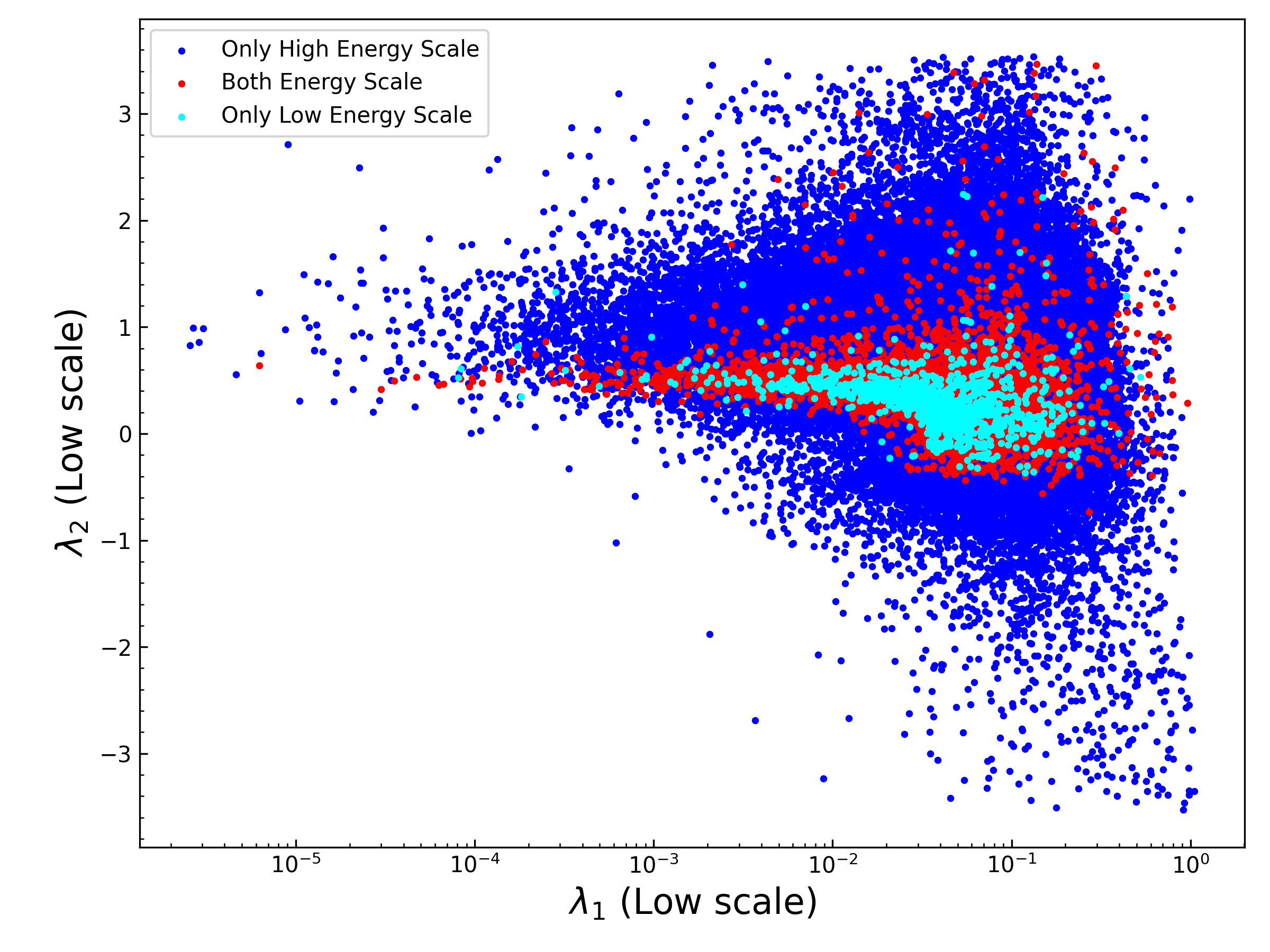
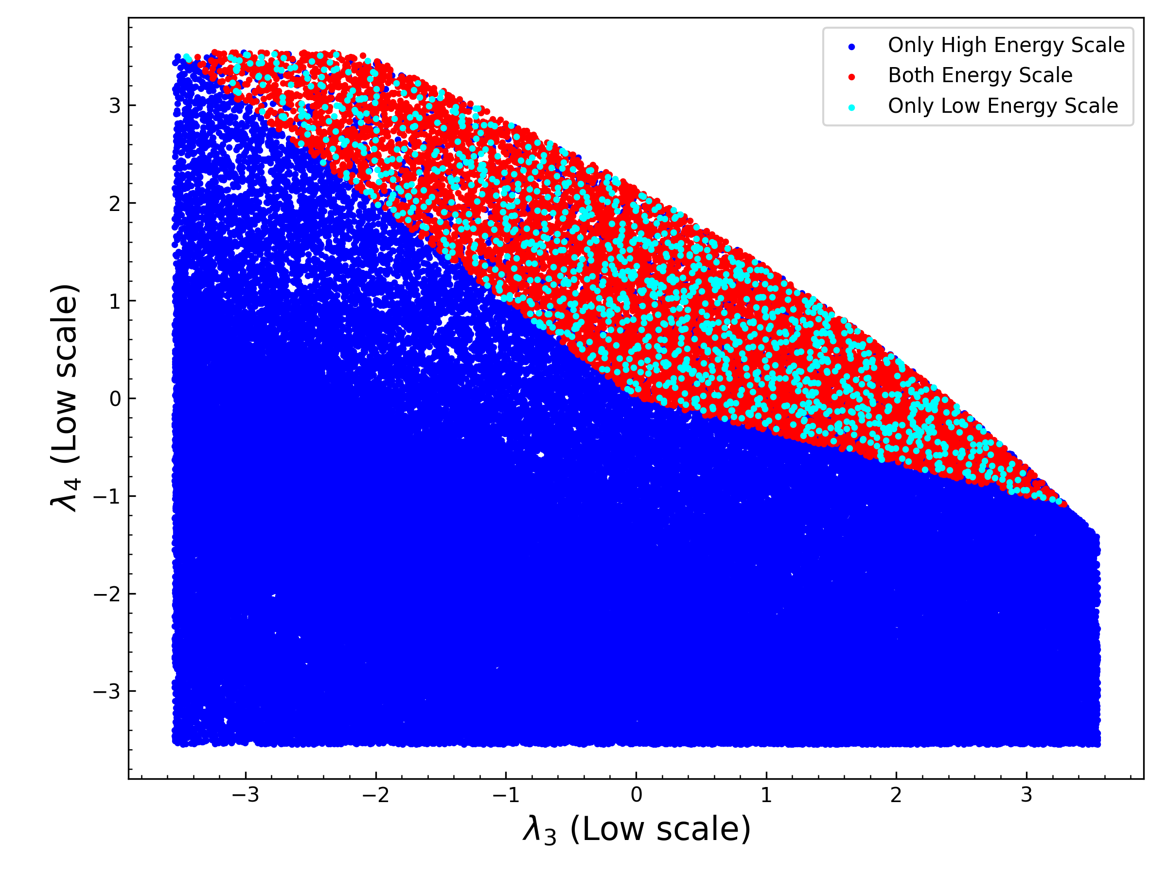
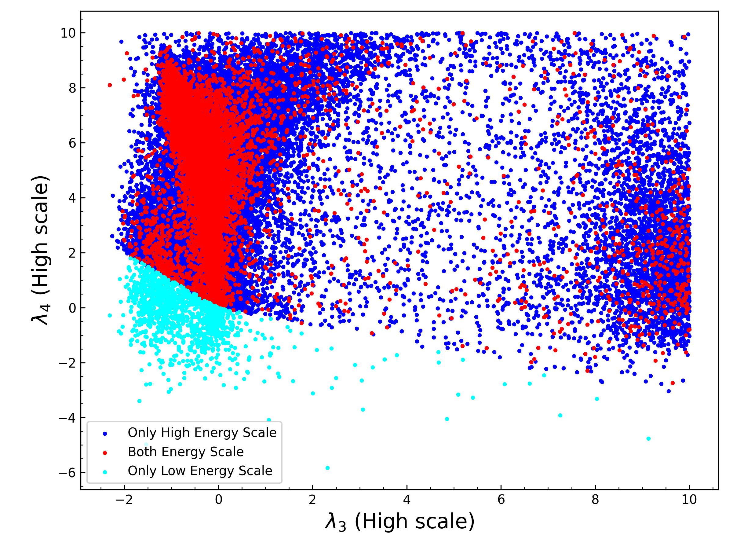
  Figure 1: Positive definiteness constraints for relevant quartic couplings. All points can fulfill the bounds of perturbative unitarity and constraints to avoid alternative minima. The blue points denote parameters that cannot guarantee the positive definiteness of scalar potential for field values at EW scale, which, however, can guarantee the positive definiteness of the scalar potential upon 10 TeV. The cyan points denote the parameters that can only satisfy the bounded-from-below condition of the scalar potential for field values at the EW scale. The red dots denote the parameters that can guarantee the positive definiteness of the effective scalar potential at all field values below the Planck/Landau pole scale. In the numerical scan, for simplicity, the Landau pole scales are defined to be the values where the relevant coupling begins to exceed 10 during RGE evolution.

• After previous discussions, we also would like to survey the status of positive definiteness constraints for realistic GM model, within which all current experimental bounds are also taken into account, such as the mass of SM-like Higgs, the couplings of Higgs to vector bosons and fermions ATLAS:kappaWZ ; CMS:kappaWZ ; ParticleDataGroup:2022pth , the rare B mesons decay that are sensitive to new physics B-physics . The particle spectrum, branching ratios and total widths of the scalars are generated with the package GMCALC GMCal (a calculator specifically designed for the GM model) or the package SPheno SPheno1 ; SPheno2 (which can calculate the spectrum of general new physics models when combined with SARAH SARAH1 ; SARAH2 ; SARAH3 ; SARAH4 ; SARAH5 ). Given that additional Higgs bosons in the GM model can lead to rich phenomenology, the package HiggsBounds-5.10.0 HiggsBounds1 ; HiggsBounds2 ; HiggsBounds3 ; HiggsBounds4 is adopted to ensure that relevant parameter choices can survive the bounds on additional Higgs at colliders. Besides, the package HiggsSignals-2.6.2 HiggsSignals1 ; HiggsSignals2 ; HiggsSignals3 ; HiggsTools is used to guarantee that the lightest or next-to lightest CP-even Higgs boson behaves like the SM-like Higgs.

  In addition to the free input parameters $\lambda_{1,2,3,4,5}$ and $\sin{\theta}$ that adopted in the previous scenario, we also need the cubic coupling parameters $M_{1,2}$, which we set to lie between 50 GeV to 1000 GeV for realistic model inputs. The mass parameters for doublet and triplets can be determined by the tadpole conditions. Once a set of parameters that satisfy all theoretical and experimental constraints are specified, we will RGE evolve those parameters to Planck scale or the corresponding Landau pole scale. With the one-loop RG-improved scalar potential, the positive definiteness bounds can be derived for the set of input parameters.

  We present a benchmark point to show the effects of RGE for the quartic couplings in Table 1, which can satisfy both current experimental and theoretical constraints except the bounded-from-below constraints adopted in previous studies. It is obvious that some of the quartic couplings will be promoted to large values by RGE, changing substantially the landscape of the scalar potential in the large field value regions.

  EW scale
  $\lambda_{1}$	0.0430	$\lambda$	0.1722	$\sigma_{4}$	0.7397
  $\lambda_{2}$	-0.5783	$\rho_{1}$	-0.1764	$\mu_{1}$	199.7229
  $\lambda_{3}$	0.3561	$\rho_{2}$	-1.4246	$\mu_{2}$	199.7229
  $\lambda_{4}$	-0.1466	$\rho_{3}$	-0.4443	$\mu_{3}$	-3868.9796
  $\lambda_{5}$	-0.5231	$\rho_{4}$	-1.1566	$m_{\phi}$	74.5236
  $M_{1}$	282.0764	$\rho_{5}$	1.4246	$m_{\xi}$	777.9569
  $M_{2}$	456.1481	$\sigma_{1}$	-1.1094	$m_{\chi}$	789.2162
  $\sin(\theta_{H})$	0.0859	$\sigma_{2}$	1.0462	$\upsilon_{\Delta}$	7.4695
  		$\sigma_{3}$	-0.2932	$\upsilon_{\phi}$	246.5897

  High energy scale ($2\times 10^{18}$GeV)
  $\lambda$	32.9029	$\sigma_{1}$	1.2304
  $\rho_{1}$	1.5356	$\sigma_{2}$	0.8382
  $\rho_{2}$	-0.6494	$\sigma_{3}$	0.9522
  $\rho_{3}$	1.4619	$\sigma_{4}$	0.4982
  $\rho_{4}$	1.4289	$min(\delta_{i})$	0.0556
  $\rho_{5}$	3.5966	$max(\delta_{i})$	2.9472

  Observeables
  $m_{h_{1}}$	124.8515	$m_{H^{\pm}_{3}}$	886.0816	$\kappa_{ww}$	1.0056
  $m_{h_{2}}$	887.8551	$m_{H^{\pm\pm}}$	884.5776	$\kappa_{zz}$	1.0056
  $m_{h_{3}}$	894.3810	$\kappa_{tt}$	0.9980	$\kappa_{\gamma\gamma}$	1.0553
  $m_{a_{2}}$	894.1385	$\kappa_{bb}$	0.9980	S	-0.0046
  $m_{H^{\pm}_{2}}$	884.6342	$\kappa_{\tau\tau}$	0.9980	T	-0.0019

  Observeables
  U	-0.0005	HiggsSignals	$\checkmark$
  $Br(B_{s}\rightarrow X_{S}\gamma)$	$3.1470\times{10}^{-4}$	Unitarity	$\checkmark$
  $Br(B_{s}\rightarrow\mu^{+}\mu^{-})$	$3.0978\times{10}^{-9}$	VS at EW	$\times$
  $Br(B^{+}\rightarrow\tau^{+}\nu)$	$1.2283\times{10}^{-4}$	VS at High scale	$\checkmark$
  HiggsBounds	$\checkmark$	Positive Definiteness	$\checkmark$

  Table 1: A Benchmark point for realistic GM model. The first table shows the input parameters in (7) and the corresponding values in the scalar potential (44) at the EW scale. The values in the second table are the RGE evolved ones for the corresponding parameters in the first table, with the RGE terminated at $2\times 10^{18}$ GeV. We also present some of the low energy experimental observables in the third and fourth tables. The unit for all parameters with mass dimension listed in the table is GeV.

  

  

  

  

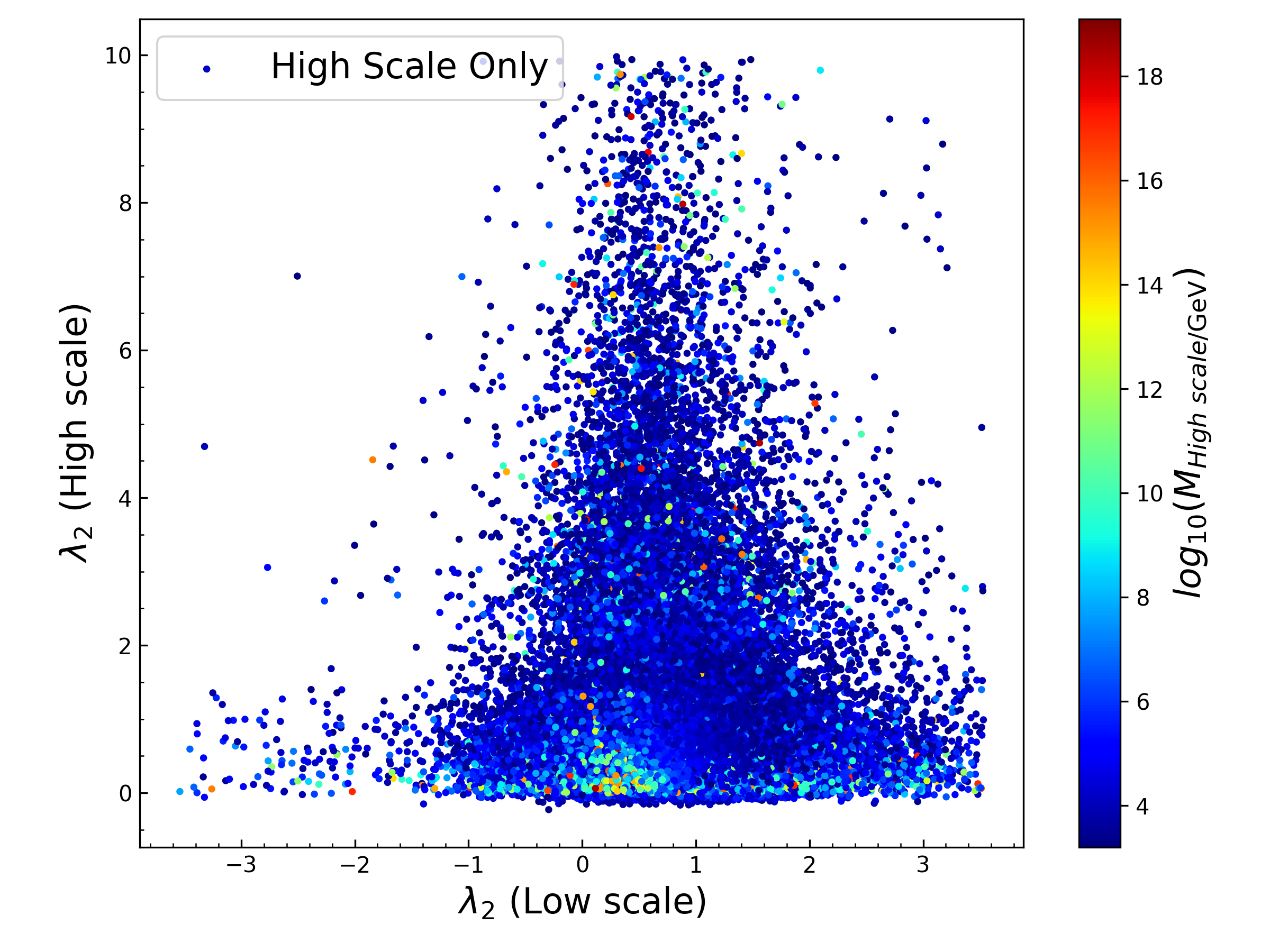
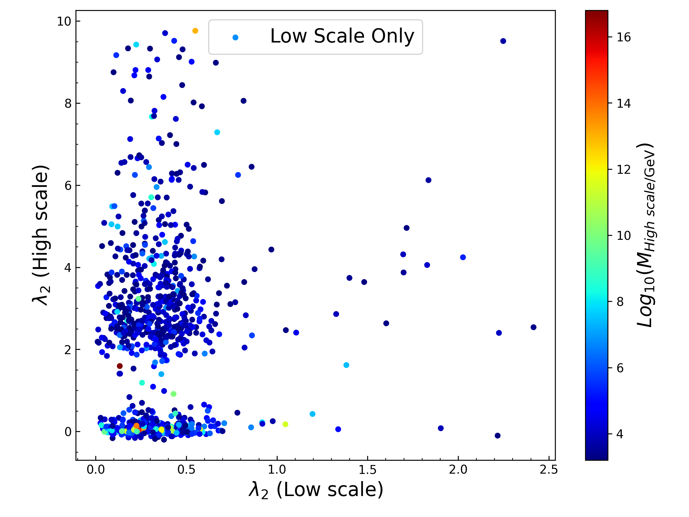
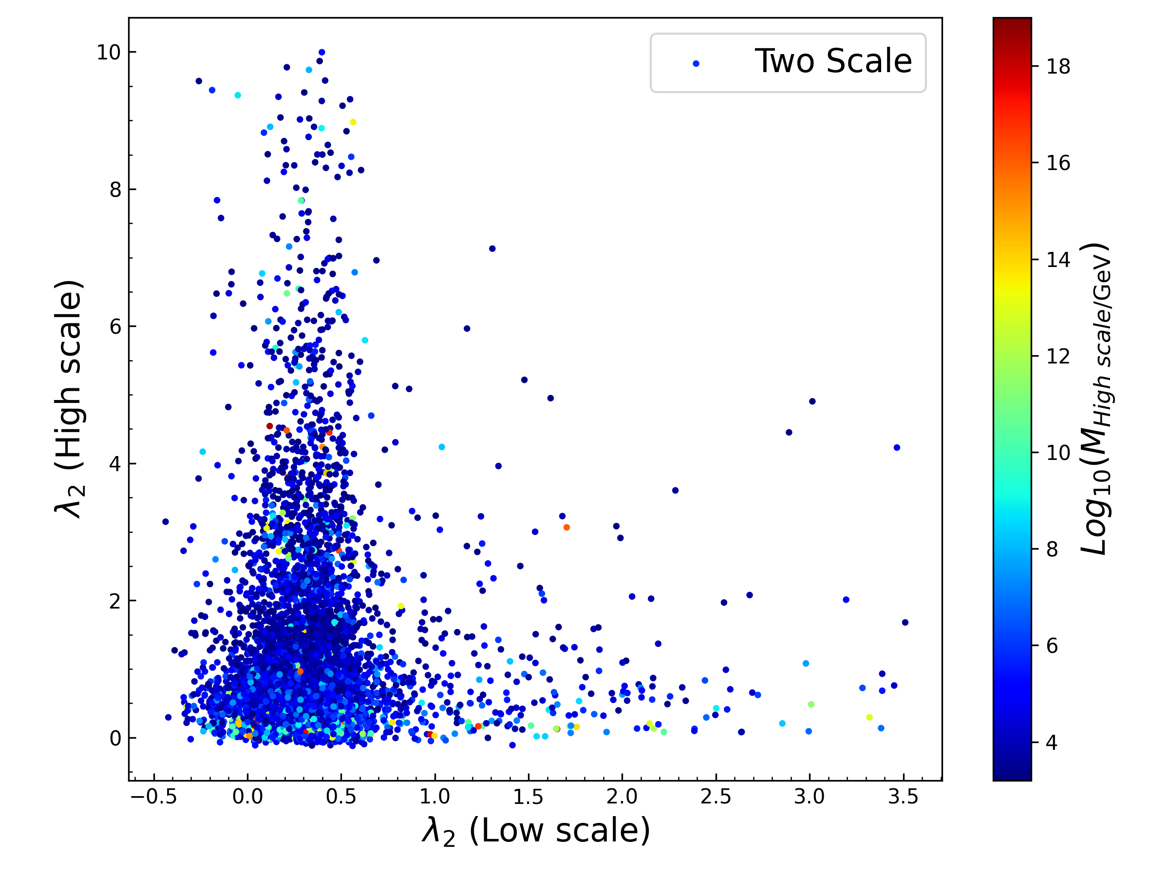
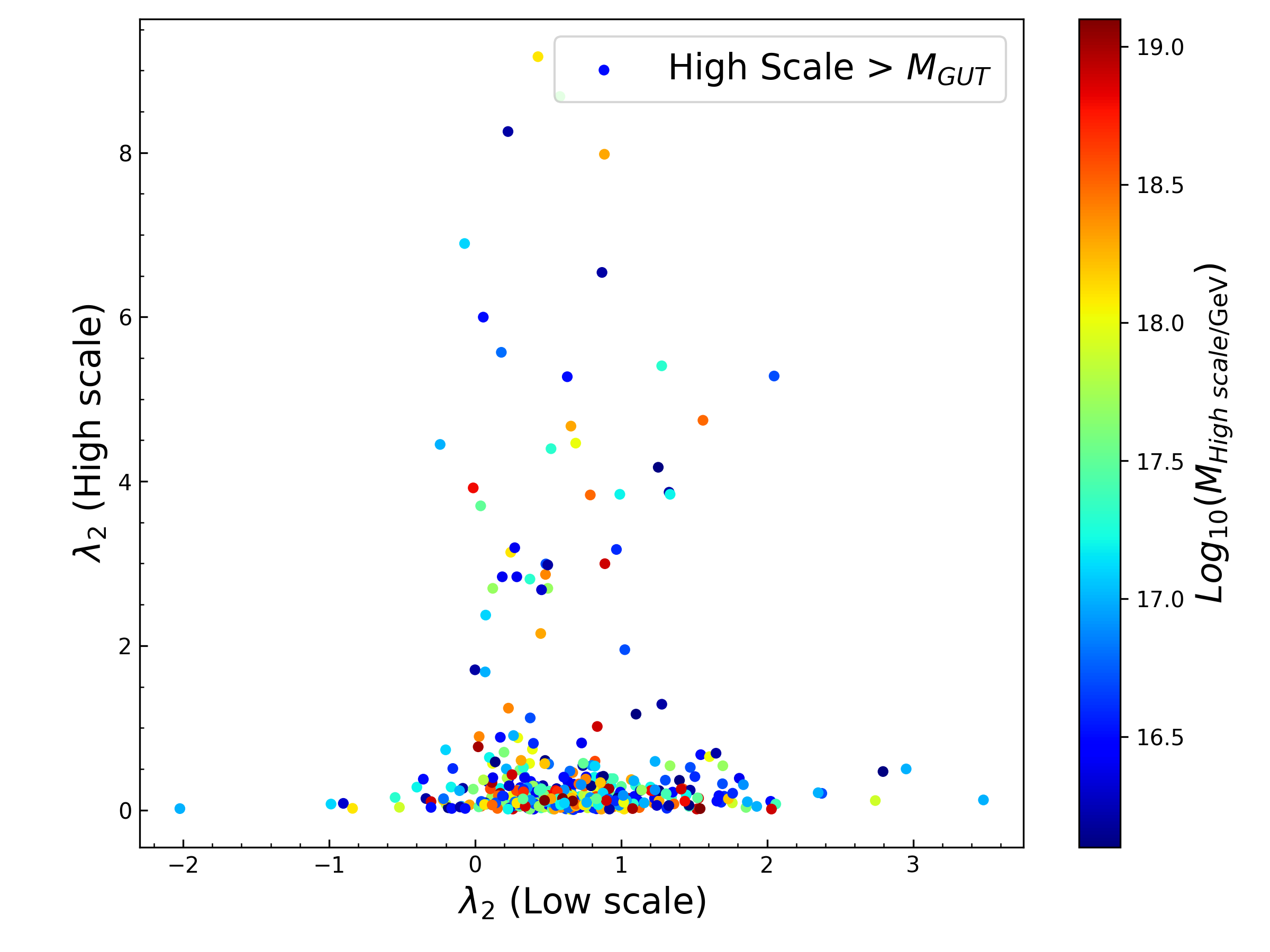
  Figure 2: The values of quartic couplings (here the $\lambda_{2}$ coupling) at the EW scale and at typical high energy scale after RGE for various cases. Different colors correspond to different maximum scales each input parameter point can achieve by RGE. In the panels (a-c), we show the quartic coupling values of the survived paramter points that can guarantee the positive definiteness of scalar potential for field values upon 10 TeV, at the EW scale only, and at all field values, respectively. Panel (d) shows the parameter points that can guarantee the positive definiteness of scalar potential up to the Planck scale.

  We also scan numerically the parameter points to survey the positive definiteness constraints in realistic GM model. Our numerical results are presented in Fig.2, within which all points must satisfy both current experimental and theoretical constraints except the bounded-from-below constraints adopted in previous studies. In those four panels, we show the values of quartic couplings (here we choose the $\lambda_{2}$ coupling to illustrate the effects of RGE) at the EW scale and at typical high energy scale after RGE for various cases. Different colors correspond to different maximum scales (reaching corresponding Landau pole scale for typical quartic coupling or reaching the Planck scale) that each input parameter point can achieve by RGE. We show the corresponding quartic coupling values of the survived paramter points that can guarantee the positive definiteness of effective scalar potential for field values upon 10 TeV, at the EW scale only, and at all field values in the upper left, upper right and the lower left panels, respectively. It can be seen from the panels that the parameter region that can guarantee the positive definiteness of scalar potential for field values upon 10 TeV is significantly larger than the previously adopted tree-level bounded-from-below condition (which is based on the quartic values defined at the EW scale). Only a portion of parameter space can guarantee the positive definiteness of effective scalar potential at all field values. We should note that the positive definiteness bounds at high energies (upon 10 TeV) can readily guarantee the theoretical consistency of the model, ensuring the non-existence of a deeper vacuum in various large field value regions. So, the parameter points in the upper left panel after substracting those of the low left panel should be re-included in realistic phenomenological discussions, which illustrate the importance of the positive definiteness bounds beyond tree-level considerations. Some of their predictions can be tested in the future colliders, such as HL-LHC HL-LHC and CEPC CEPC .

  Some parameter points can guarantee the positive definiteness of scalar potential up to the Planck scale, indicating that the theory can be well defined up to the quantum gravity scale, which will neither reach any Landau pole nor lead to additional deeper vacua (or the potential energy not bounded from below at all) at large field values below $M_{Pl}$. Such parameter points are shown in the lower right panel.

5 Conclusions

The tree-level bounded-from-below constraints for the GM model, obtained by requiring the scalar potential to be positive definite for EW scale quartic couplings, can set stringent constraints on the input parameters in phenomenological studies. However, the landscape of effective scalar potential can be quite different from the tree-level scalar potential, rendering the previously adopted tree-level bounded-from-below constraints not very reliable. For large field values, the one-loop RG-improved tree-level scalar potential can be adopted to approximate the effective potential for our analysis of the positive definiteness constraints. Because the custodial symmetry will be broken by loop effect involving the hypercharge gauge interactions, some custodial violating terms will appear again in the scalar potential, necessitating new positive definite criterion for the effective scalar potential that takes a multiple variable polynomial form.

We scan numerically the parameter points to analyse the positive definiteness constraints with new positive definite criteria for homogeneous polynomials with multiple variables, ensuring the non-existence of a deeper vacuum in large field value regions. We find that, many parameter points, which are excluded by previous (tree-level) bounded-from-below constraints, can still satisfy the positive definiteness constraints for the scalar potential with the one-loop RG-improved scalar potential in large field value regions. Besides, a portion of parameter space that can satisfy the tree-level bounded-from-below constraints (with EW scale coupling inputs), should in fact be ruled out by the the positive definiteness constraints of the effective potential at large field value regions.

We should note that we do not consider the case with a meta-stable electroweak vacuum. As long as the lifetime for the meta-stable vacuum is longer than the age of our universe, such a meta-stable vacuum will not cause a problem. Because the GM model has a rich vacuum structure, many false vacua (such as charge breaking minimum or wrong electroweak minimum) can co-exist with the true vacuum, leading to multiple step transitions to the true minimum. So, unless we know the vacuum structure of the effective potential at large field value regions, the naive estimation of the lifetime for meta-stable eletroweak vacuum by calculating its transition rate to the true vacuum is always not reliable. We would like to discuss further the vacuum structure of the effective potential in our future works.

Appendix A One-loop $\beta$-functions for GM model

In our numerical studies, beta functions for various couplings are needed for RGE of the relevant parameters. The one-loop $\beta$-functions for the gauge couplings $g_{1,2,3}$, the Yukawa couplings $Y_{u,d,e}$ and quartic couplings $\lambda$, $\rho_{1,2,3,4,5}$,$\sigma_{1,2,3,4}$, are given respectively as

$$\beta_{g_{1}} = ~{}\frac{47}{10}g_{1}^{3},~{}~{}~{}\beta_{g_{2}}=-\frac{13}{6}g_{2}^{3},~{}~{}~{}\beta_{g_{3}}=-7g_{3}^{3},~{}~{}~{}~{}~{}~{}~{}~{}~{}~{}~{}~{}~{}~{}~{}~{}~{}~{}~{}~{}~{}~{}~{}~{}~{}~{}~{}~{}~{}~{}~{}~{}~{}~{}~{}~{}~{}~{}~{}~{}~{}$$ (101)

$$\beta_{Y_{u}} = -\frac{3}{2}\Big{(}-{Y_{u}Y_{u}^{\dagger}Y_{u}}+{Y_{u}Y_{d}^{\dagger}Y_{d}}\Big{)}$$ (102)

$$+ Y_{u}\Big{(}3\mbox{Tr}\Big{(}{Y_{d}Y_{d}^{\dagger}}\Big{)}+3\mbox{Tr}\Big{(}{Y_{u}Y_{u}^{\dagger}}\Big{)}-8g_{3}^{2}-\frac{17}{20}g_{1}^{2}-\frac{9}{4}g_{2}^{2}+\mbox{Tr}\Big{(}{Y_{e}Y_{e}^{\dagger}}\Big{)}\Big{)},$$

$$\beta_{Y_{d}} = \frac{1}{4}\Big{(}6\Big{(}-{Y_{d}Y_{u}^{\dagger}Y_{u}}+{Y_{d}Y_{d}^{\dagger}Y_{d}}\Big{)}$$ (103)

$$- Y_{d}\Big{(}-12\mbox{Tr}\Big{(}{Y_{d}Y_{d}^{\dagger}}\Big{)}-12\mbox{Tr}\Big{(}{Y_{u}Y_{u}^{\dagger}}\Big{)}+32g_{3}^{2}-4\mbox{Tr}\Big{(}{Y_{e}Y_{e}^{\dagger}}\Big{)}+9g_{2}^{2}+g_{1}^{2}\Big{)}\Big{)},$$

$$\beta_{Y_{e}} = \frac{3}{2}{Y_{e}Y_{e}^{\dagger}Y_{e}}+Y_{e}\Big{(}3\mbox{Tr}\Big{(}{Y_{d}Y_{d}^{\dagger}}\Big{)}+3\mbox{Tr}\Big{(}{Y_{u}Y_{u}^{\dagger}}\Big{)}-\frac{9}{4}g_{1}^{2}-\frac{9}{4}g_{2}^{2}+\mbox{Tr}\Big{(}{Y_{e}Y_{e}^{\dagger}}\Big{)}\Big{)},$$ (104)

and

$$\beta_{{\lambda}_{1}} = \frac{27}{200}g_{1}^{4}+\frac{9}{20}g_{1}^{2}g_{2}^{2}+\frac{9}{8}g_{2}^{4}-\frac{9}{5}g_{1}^{2}{\lambda}_{1}-9g_{2}^{2}{\lambda}_{1}+24{\lambda}_{1}^{2}+3{\sigma}_{1}^{2}+3{\sigma}_{1}{\sigma}_{2}+\frac{5}{4}{\sigma}_{2}^{2}+6{\sigma}_{3}^{2}$$ (105)

$$+ 2|{\sigma}_{4}|^{2}+12{\lambda}_{1}\mbox{Tr}\Big{(}{Y_{d}Y_{d}^{\dagger}}\Big{)}+4{\lambda}_{1}\mbox{Tr}\Big{(}{Y_{e}Y_{e}^{\dagger}}\Big{)}+12{\lambda}_{1}\mbox{Tr}\Big{(}{Y_{u}Y_{u}^{\dagger}}\Big{)}-6\mbox{Tr}\Big{(}{Y_{d}Y_{d}^{\dagger}Y_{d}Y_{d}^{\dagger}}\Big{)}$$

$$- 2\mbox{Tr}\Big{(}{Y_{e}Y_{e}^{\dagger}Y_{e}Y_{e}^{\dagger}}\Big{)}-6\mbox{Tr}\Big{(}{Y_{u}Y_{u}^{\dagger}Y_{u}Y_{u}^{\dagger}}\Big{)},$$

$$\beta_{{\sigma}_{1}} = \frac{27}{25}g_{1}^{4}-\frac{18}{5}g_{1}^{2}g_{2}^{2}+6g_{2}^{4}-\frac{9}{2}g_{1}^{2}{\sigma}_{1}-\frac{33}{2}g_{2}^{2}{\sigma}_{1}+12{\lambda}_{1}{\sigma}_{1}+16{\rho}_{1}{\sigma}_{1}+12{\rho}_{2}{\sigma}_{1}+4{\sigma}_{1}^{2}$$ (106)

$$+ 4{\lambda}_{1}{\sigma}_{2}+6{\rho}_{1}{\sigma}_{2}+2{\rho}_{2}{\sigma}_{2}+{\sigma}_{2}^{2}+12{\rho}_{4}{\sigma}_{3}+4{\rho}_{5}{\sigma}_{3}+2|{\sigma}_{4}|^{2}+6{\sigma}_{1}\mbox{Tr}\Big{(}{Y_{d}Y_{d}^{\dagger}}\Big{)}$$

$$+ 2{\sigma}_{1}\mbox{Tr}\Big{(}{Y_{e}Y_{e}^{\dagger}}\Big{)}+6{\sigma}_{1}\mbox{Tr}\Big{(}{Y_{u}Y_{u}^{\dagger}}\Big{)},$$

$$\beta_{{\sigma}_{2}} = \frac{36}{5}g_{1}^{2}g_{2}^{2}-\frac{9}{2}g_{1}^{2}{\sigma}_{2}-\frac{33}{2}g_{2}^{2}{\sigma}_{2}+4{\lambda}_{1}{\sigma}_{2}+4{\rho}_{1}{\sigma}_{2}+8{\rho}_{2}{\sigma}_{2}+8{\sigma}_{1}{\sigma}_{2}+4{\sigma}_{2}^{2}+4|{\sigma}_{4}|^{2}$$ (107)

$$+ 6{\sigma}_{2}\mbox{Tr}\Big{(}{Y_{d}Y_{d}^{\dagger}}\Big{)}+2{\sigma}_{2}\mbox{Tr}\Big{(}{Y_{e}Y_{e}^{\dagger}}\Big{)}+6{\sigma}_{2}\mbox{Tr}\Big{(}{Y_{u}Y_{u}^{\dagger}}\Big{)},$$

$$\beta_{{\sigma}_{3}} = 3g_{2}^{4}+6{\rho}_{4}{\sigma}_{1}+2{\rho}_{5}{\sigma}_{1}+3{\rho}_{4}{\sigma}_{2}+{\rho}_{5}{\sigma}_{2}-\frac{9}{10}g_{1}^{2}{\sigma}_{3}-\frac{33}{2}g_{2}^{2}{\sigma}_{3}+12{\lambda}_{1}{\sigma}_{3}+20{\rho}_{3}{\sigma}_{3}$$ (108)

$$+ 8{\sigma}_{3}^{2}+4|{\sigma}_{4}|^{2}+6{\sigma}_{3}\mbox{Tr}\Big{(}{Y_{d}Y_{d}^{\dagger}}\Big{)}+2{\sigma}_{3}\mbox{Tr}\Big{(}{Y_{e}Y_{e}^{\dagger}}\Big{)}+6{\sigma}_{3}\mbox{Tr}\Big{(}{Y_{u}Y_{u}^{\dagger}}\Big{)},$$

$$\beta_{{\sigma}_{4}} = -\frac{27}{10}g_{1}^{2}{\sigma}_{4}-\frac{33}{2}g_{2}^{2}{\sigma}_{4}+4{\lambda}_{1}{\sigma}_{4}+4{\rho}_{4}{\sigma}_{4}-2{\rho}_{5}{\sigma}_{4}+4{\sigma}_{1}{\sigma}_{4}+4{\sigma}_{2}{\sigma}_{4}+8{\sigma}_{3}{\sigma}_{4}\quad\quad$$ (109)

$$+ 6{\sigma}_{4}\mbox{Tr}\Big{(}{Y_{d}Y_{d}^{\dagger}}\Big{)}+2{\sigma}_{4}\mbox{Tr}\Big{(}{Y_{e}Y_{e}^{\dagger}}\Big{)}+6{\sigma}_{4}\mbox{Tr}\Big{(}{Y_{u}Y_{u}^{\dagger}}\Big{)},$$

$$\beta_{{\rho}_{1}} = 15g_{2}^{4}-24g_{2}^{2}{\rho}_{1}+24{\rho}_{1}{\rho}_{2}+28{\rho}_{1}^{2}+2{\sigma}_{1}^{2}+2{\sigma}_{1}{\sigma}_{2}+3{\rho}_{5}^{2}+4{\rho}_{4}{\rho}_{5}+6{\rho}_{2}^{2}+6{\rho}_{4}^{2}\quad$$ (110)

$$- \frac{36}{5}g_{1}^{2}\Big{(}g_{2}^{2}+{\rho}_{1}\Big{)}+\frac{54}{25}g_{1}^{4},$$

$$\beta_{{\rho}_{2}} = 18{\rho}_{2}^{2}-24g_{2}^{2}{\rho}_{2}+24{\rho}_{1}{\rho}_{2}-2{\rho}_{5}^{2}-6g_{2}^{4}+\frac{36}{5}g_{1}^{2}\Big{(}2g_{2}^{2}-{\rho}_{2}\Big{)}+{\sigma}_{2}^{2},~{}~{}~{}~{}~{}~{}~{}~{}~{}~{}~{}~{}~{}~{}~{}~{}~{}$$ (111)

$$\beta_{{\rho}_{3}} = 2\Big{(}-12g_{2}^{2}{\rho}_{3}+22{\rho}_{3}^{2}+2{\rho}_{4}{\rho}_{5}+2{\sigma}_{3}^{2}+3g_{2}^{4}+3{\rho}_{4}^{2}+{\rho}_{5}^{2}\Big{)},~{}~{}~{}~{}~{}~{}~{}~{}~{}~{}~{}~{}~{}~{}~{}~{}~{}~{}~{}~{}~{}~{}~{}~{}~{}$$ (112)

$$\beta_{{\rho}_{4}} = 6g_{2}^{4}-\frac{18}{5}g_{1}^{2}{\rho}_{4}-24g_{2}^{2}{\rho}_{4}+16{\rho}_{1}{\rho}_{4}+12{\rho}_{2}{\rho}_{4}+20{\rho}_{3}{\rho}_{4}+8{\rho}_{4}^{2}+4{\rho}_{1}{\rho}_{5}+4{\rho}_{2}{\rho}_{5}$$ (113)

$$+ 4{\rho}_{3}{\rho}_{5}+2{\rho}_{5}^{2}+4{\sigma}_{1}{\sigma}_{3}+2{\sigma}_{2}{\sigma}_{3}+2|{\sigma}_{4}|^{2},$$

$$\beta_{{\rho}_{5}} = -24g_{2}^{2}{\rho}_{5}+2{\rho}_{5}\Big{(}2{\rho}_{1}+4{\rho}_{3}+5{\rho}_{5}+8{\rho}_{4}\Big{)}-2|{\sigma}_{4}|^{2}+6g_{2}^{4}-\frac{18}{5}g_{1}^{2}{\rho}_{5},\quad\quad\quad\quad$$ (114)

with

$$\frac{d}{d\ln\mu}\tilde{\lambda}=\frac{1}{16\pi^{2}}\beta_{\tilde{\lambda}}~{},$$ (115)

for any coupling $\tilde{\lambda}$. It should be noted that the $\beta$ function for $U(1)_{Y}$ gauge coupling $g_{1}$ differs by a normalization factor $3/5$ from that given in GM44 , in which the GUT normalization $5g_{1}^{2}=3({g^{\prime}})^{2}$ is adopted.

For completeness, the beta function for dimensional couplings are also list here

$$\beta_{\mu} = -\frac{27}{10}g_{1}^{2}\mu-\frac{21}{2}g_{2}^{2}\mu+4{\lambda}_{1}\mu+4\mu{\sigma}_{1}+6\mu{\sigma}_{2}+\Big{(}-2{\mu}_{3}+4{\mu}_{1}\Big{)}{\sigma}_{4}^{*}+6\mu\mbox{Tr}\Big{(}{Y_{d}Y_{d}^{\dagger}}\Big{)}$$ (116)

$$+ 2\mu\mbox{Tr}\Big{(}{Y_{e}Y_{e}^{\dagger}}\Big{)}+6\mu\mbox{Tr}\Big{(}{Y_{u}Y_{u}^{\dagger}}\Big{)},$$

$$\beta_{{\mu}_{1}} = -\frac{9}{10}g_{1}^{2}{\mu}_{1}-\frac{21}{2}g_{2}^{2}{\mu}_{1}+4{\lambda}_{1}{\mu}_{1}-2{\mu}_{3}{\sigma}_{2}+8{\mu}_{1}{\sigma}_{3}+8\mu{\sigma}_{4}+8\mu^{*}{\sigma}_{4}^{*}+6{\mu}_{1}\mbox{Tr}\Big{(}{Y_{d}Y_{d}^{\dagger}}\Big{)}$$ (117)

$$+ 2{\mu}_{1}\mbox{Tr}\Big{(}{Y_{e}Y_{e}^{\dagger}}\Big{)}+6{\mu}_{1}\mbox{Tr}\Big{(}{Y_{u}Y_{u}^{\dagger}}\Big{)},$$

$$\beta_{{\mu}_{3}} = -18g_{2}^{2}{\mu}_{3}-2{\mu}_{1}{\sigma}_{2}+4{\mu}_{3}{\rho}_{1}-4{\mu}_{3}{\rho}_{5}-4\mu^{*}{\sigma}_{4}^{*}-4\mu{\sigma}_{4}+8{\mu}_{3}{\rho}_{2}+8{\mu}_{3}{\rho}_{4}-\frac{18}{5}g_{1}^{2}{\mu}_{3},$$

$$\beta_{m^{2}_{\xi}} = 2\Big{(}10m^{2}_{\xi}{\rho}_{3}+2m^{2}_{\chi}{\rho}_{5}+4m^{2}_{\phi}{\sigma}_{3}-6g_{2}^{2}m^{2}_{\xi}+6m^{2}_{\chi}{\rho}_{4}+{\mu}_{1}^{2}+{\mu}_{3}^{2}\Big{)},$$ (119)

$$\beta_{m^{2}_{\phi}} = -\frac{9}{10}g_{1}^{2}m^{2}_{\phi}-\frac{9}{2}g_{2}^{2}m^{2}_{\phi}+12{\lambda}_{1}m^{2}_{\phi}+3{\mu}_{1}^{2}+6m^{2}_{\chi}{\sigma}_{1}+3m^{2}_{\chi}{\sigma}_{2}+6m^{2}_{\xi}{\sigma}_{3}+12|\mu|^{2}$$ (120)

$$+ 6m^{2}_{\phi}\mbox{Tr}\Big{(}{Y_{d}Y_{d}^{\dagger}}\Big{)}+2m^{2}_{\phi}\mbox{Tr}\Big{(}{Y_{e}Y_{e}^{\dagger}}\Big{)}+6m^{2}_{\phi}\mbox{Tr}\Big{(}{Y_{u}Y_{u}^{\dagger}}\Big{)},$$

$$\beta_{m^{2}_{\chi}} = -12g_{2}^{2}m^{2}_{\chi}+12m^{2}_{\chi}{\rho}_{2}+16m^{2}_{\chi}{\rho}_{1}+2m^{2}_{\xi}{\rho}_{5}+2m^{2}_{\phi}{\sigma}_{2}+2{\mu}_{3}^{2}+4m^{2}_{\phi}{\sigma}_{1}+4|\mu|^{2}\quad\quad\quad$$ (121)

$$+ 6m^{2}_{\xi}{\rho}_{4}-\frac{18}{5}g_{1}^{2}m^{2}_{\chi}.$$

References

- (1) G. Aad et al. [ATLAS], Phys. Lett. B 710 (2012), 49-66 doi:10.1016/j.physletb.2012.02.044 [arXiv:1202.1408 [hep-ex]].
- (2) S. Chatrchyan et al. [CMS], Phys. Lett. B 710 (2012), 26-48 doi:10.1016/j.physletb.2012.02.064 [arXiv:1202.1488 [hep-ex]].
- (3) H. Georgi and M. Machacek, Nucl. Phys. B 262 (1985), 463-477 doi:10.1016/0550-3213(85)90325-6.
- (4) M. S. Chanowitz and M. Golden, Phys. Lett. B 165 (1985), 105-108 doi:10.1016/0370-2693(85)90700-2.
- (5) J. F. Gunion, R. Vega and J. Wudka, Phys. Rev. D 42 (1990), 1673-1691 doi:10.1103/PhysRevD.42.1673.
- (6) J. F. Gunion, R. Vega and J. Wudka, Phys. Rev. D 43 (1991), 2322-2336 doi:10.1103/PhysRevD.43.2322.
- (7) J. F. Gunion, H. E. Haber, G. L. Kane and S. Dawson, Front. Phys. 80 (2000), 1-404 SCIPP-89/13.
- (8) H. E. Haber and H. E. Logan, Phys. Rev. D 62 (2000), 015011 doi:10.1103/PhysRevD.62.015011 [arXiv:hep-ph/9909335 [hep-ph]].
- (9) S. Godfrey and K. Moats, Phys. Rev. D 81 (2010), 075026 doi:10.1103/PhysRevD.81.075026 [arXiv:1003.3033 [hep-ph]].
- (10) I. Low, J. Lykken and G. Shaughnessy, Phys. Rev. D 86 (2012), 093012 doi:10.1103/PhysRevD.86.093012 [arXiv:1207.1093 [hep-ph]].
- (11) H. E. Logan and M. A. Roy, Phys. Rev. D 82 (2010), 115011 doi:10.1103/PhysRevD.82.115011 [arXiv:1008.4869 [hep-ph]].
- (12) R. Killick, K. Kumar and H. E. Logan, Phys. Rev. D 88 (2013), 033015 doi:10.1103/PhysRevD.88.033015 [arXiv:1305.7236 [hep-ph]].
- (13) A. Efrati and Y. Nir, [arXiv:1401.0935 [hep-ph]].
- (14) C. Degrande, K. Hartling, H. E. Logan, A. D. Peterson and M. Zaro, Phys. Rev. D 93 (2016) no.3, 035004 doi:10.1103/PhysRevD.93.035004 [arXiv:1512.01243 [hep-ph]].
- (15) C. H. de Lima and H. E. Logan, Phys. Rev. D 106 (2022) no.11, 115020 doi:10.1103/PhysRevD.106.115020 [arXiv:2209.08393 [hep-ph]].
- (16) A. Ahriche, Phys. Rev. D 107 (2023) no.1, 015006 doi:10.1103/PhysRevD.107.015006 [arXiv:2212.11579 [hep-ph]].
- (17) S. L. Chen, A. Dutta Banik and Z. K. Liu, Nucl. Phys. B 966 (2021), 115394 doi:10.1016/j.nuclphysb.2021.115394 [arXiv:2011.13551 [hep-ph]].
- (18) A. Falkowski, S. Rychkov and A. Urbano, JHEP 04 (2012), 073 doi:10.1007/JHEP04(2012)073 [arXiv:1202.1532 [hep-ph]].
- (19) S. Chang, C. A. Newby, N. Raj and C. Wanotayaroj, Phys. Rev. D 86 (2012), 095015 doi:10.1103/PhysRevD.86.095015 [arXiv:1207.0493 [hep-ph]].
- (20) C. W. Chiang, A. L. Kuo and K. Yagyu, JHEP 10 (2013), 072 doi:10.1007/JHEP10(2013)072 [arXiv:1307.7526 [hep-ph]].
- (21) Y. Yu, Y. P. Bi and J. F. Shen, Phys. Lett. B 759 (2016), 513-519 doi:10.1016/j.physletb.2016.06.014.
- (22) J. Cao and Y. B. Liu, Mod. Phys. Lett. A 31 (2016) no.32, 1650182 doi:10.1142/S0217732316501820.
- (23) H. Sun, X. Luo, W. Wei and T. Liu, Phys. Rev. D 96 (2017) no.9, 095003 doi:10.1103/PhysRevD.96.095003 [arXiv:1710.06284 [hep-ph]].
- (24) J. Cao, Y. Q. Li and Y. B. Liu, Int. J. Mod. Phys. A 33 (2018) no.11, 1841003 doi:10.1142/S0217751X18410038.
- (25) Q. Yang, R. Y. Zhang, W. G. Ma, Y. Jiang, X. Z. Li and H. Sun, Phys. Rev. D 98 (2018) no.5, 055034 doi:10.1103/PhysRevD.98.055034 [arXiv:1810.08965 [hep-ph]].
- (26) C. W. Chiang and K. Yagyu, JHEP 01 (2013), 026 doi:10.1007/JHEP01(2013)026 [arXiv:1211.2658 [hep-ph]].
- (27) S. Kanemura, M. Kikuchi and K. Yagyu, Phys. Rev. D 88 (2013), 015020 doi:10.1103/PhysRevD.88.015020 [arXiv:1301.7303 [hep-ph]].
- (28) C. Englert, E. Re and M. Spannowsky, Phys. Rev. D 87 (2013) no.9, 095014 doi:10.1103/PhysRevD.87.095014 [arXiv:1302.6505 [hep-ph]].
- (29) C. Englert, E. Re and M. Spannowsky, Phys. Rev. D 88 (2013), 035024 doi:10.1103/PhysRevD.88.035024 [arXiv:1306.6228 [hep-ph]].
- (30) S. I. Godunov, M. I. Vysotsky and E. V. Zhemchugov, J. Exp. Theor. Phys. 120 (2015) no.3, 369-375 doi:10.1134/S1063776115030073 [arXiv:1408.0184 [hep-ph]].
- (31) C. W. Chiang and K. Tsumura, JHEP 04 (2015), 113 doi:10.1007/JHEP04(2015)113 [arXiv:1501.04257 [hep-ph]].
- (32) C. W. Chiang, A. L. Kuo and T. Yamada, JHEP 01, 120 (2016) doi:10.1007/JHEP01(2016)120 [arXiv:1511.00865 [hep-ph]].
- (33) J. Chang, C. R. Chen and C. W. Chiang, JHEP 03 (2017), 137 doi:10.1007/JHEP03(2017)137 [arXiv:1701.06291 [hep-ph]].
- (34) B. Li, Z. L. Han and Y. Liao, JHEP 02 (2018), 007 doi:10.1007/JHEP02(2018)007 [arXiv:1710.00184 [hep-ph]].
- (35) N. Ghosh, S. Ghosh and I. Saha, Phys. Rev. D 101 (2020) no.1, 015029 doi:10.1103/PhysRevD.101.015029 [arXiv:1908.00396 [hep-ph]].
- (36) A. Ismail, H. E. Logan and Y. Wu, [arXiv:2003.02272 [hep-ph]].
- (37) C. Wang, J. Q. Tao, M. A. Shahzad, G. M. Chen and S. Gascon-Shotkin, Chin. Phys. C 46 (2022) no.8, 083107 doi:10.1088/1674-1137/ac6cd3 [arXiv:2204.09198 [hep-ph]].
- (38) S. Ghosh, [arXiv:2205.03896 [hep-ph]].
- (39) M. Chakraborti, D. Das, N. Ghosh, S. Mukherjee and I. Saha, Phys. Rev. D 109 (2024) no.1, 015016 doi:10.1103/PhysRevD.109.015016 [arXiv:2308.02384 [hep-ph]].
- (40) S. Ghosh, [arXiv:2311.15405 [hep-ph]].
- (41) Y. Zhang, H. Sun, X. Luo and W. Zhang, Phys. Rev. D 95 (2017) no.11, 115022 doi:10.1103/PhysRevD.95.115022 [arXiv:1706.01490 [hep-ph]].
- (42) G. Azuelos, H. Sun and K. Wang, Phys. Rev. D 97 (2018) no.11, 116005 doi:10.1103/PhysRevD.97.116005 [arXiv:1712.07505 [hep-ph]].
- (43) J. W. Zhu, R. Y. Zhang, W. G. Ma, Q. Yang, M. M. Long and Y. Jiang, J. Phys. G 47 (2020) no.12, 125005 doi:10.1088/1361-6471/abaddf.
- (44) S. Ghosh, doi:10.31526/LHEP.2024.518 [arXiv:2311.15405 [hep-ph]].
- (45) A. Ahriche, [arXiv:2312.10484 [hep-ph]].
- (46) T. K. Chen, C. W. Chiang, S. Heinemeyer and G. Weiglein, Phys. Rev. D 109 (2024) no.7, 075043 doi:10.1103/PhysRevD.109.075043 [arXiv:2312.13239 [hep-ph]].
- (47) S. Blasi, S. De Curtis and K. Yagyu, Phys. Rev. D 96, no.1, 015001 (2017) doi:10.1103/PhysRevD.96.015001 [arXiv:1704.08512 [hep-ph]].
- (48) B. Keeshan, H. E. Logan and T. Pilkington, Phys. Rev. D 102 (2020) no.1, 015001 doi:10.1103/PhysRevD.102.015001 [arXiv:1807.11511 [hep-ph]].
- (49) H. Song, X. Wan and J. H. Yu, Chin. Phys. C 47 (2023) no.10, 103103 doi:10.1088/1674-1137/ace5a6 [arXiv:2211.01543 [hep-ph]].
- (50) R. Ghosh and B. Mukhopadhyaya, Phys. Rev. D 107 (2023) no.3, 035031 doi:10.1103/PhysRevD.107.035031 [arXiv:2212.11688 [hep-ph]].
- (51) X. K. Du, Z. Li, F. Wang and Y. K. Zhang, Eur. Phys. J. C 83 (2023) no.2, 139 doi:10.1140/epjc/s10052-023-11297-1 [arXiv:2204.05760 [hep-ph]].
- (52) P. Mondal, Phys. Lett. B 833 (2022), 137357 doi:10.1016/j.physletb.2022.137357 [arXiv:2204.07844 [hep-ph]].
- (53) T. K. Chen, C. W. Chiang and K. Yagyu, Phys. Rev. D 106 (2022) no.5, 055035 doi:10.1103/PhysRevD.106.055035 [arXiv:2204.12898 [hep-ph]].
- (54) R. Ghosh, B. Mukhopadhyaya and U. Sarkar, J. Phys. G 50 (2023) no.7, 075003 doi:10.1088/1361-6471/acd0c8 [arXiv:2205.05041 [hep-ph]].
- (55) C. W. Chiang and T. Yamada, Phys. Lett. B 735 (2014), 295-300 doi:10.1016/j.physletb.2014.06.048 [arXiv:1404.5182 [hep-ph]].
- (56) T. K. Chen, C. W. Chiang, C. T. Huang and B. Q. Lu, Phys. Rev. D 106 (2022) no.5, 055019 doi:10.1103/PhysRevD.106.055019 [arXiv:2205.02064 [hep-ph]].
- (57) R. Zhou, W. Cheng, X. Deng, L. Bian and Y. Wu, JHEP 01 (2019), 216 doi:10.1007/JHEP01(2019)216 [arXiv:1812.06217 [hep-ph]].
- (58) L. Bian, H. K. Guo, Y. Wu and R. Zhou, Phys. Rev. D 101 (2020) no.3, 035011 doi:10.1103/PhysRevD.101.035011 [arXiv:1906.11664 [hep-ph]].
- (59) K. Hartling, K. Kumar and H. E. Logan, Phys. Rev. D 91 (2015) no.1, 015013 doi:10.1103/PhysRevD.91.015013 [arXiv:1410.5538 [hep-ph]].
- (60) M. Aoki and S. Kanemura, Phys. Rev. D 77 (2008) no.9, 095009 [erratum: Phys. Rev. D 89 (2014) no.5, 059902] doi:10.1103/PhysRevD.77.095009 [arXiv:0712.4053 [hep-ph]].
- (61) K. Hartling, K. Kumar and H. E. Logan, Phys. Rev. D 90 (2014) no.1, 015007 doi:10.1103/PhysRevD.90.015007 [arXiv:1404.2640 [hep-ph]].
- (62) C. W. Chiang, G. Cottin and O. Eberhardt, Phys. Rev. D 99 (2019) no.1, 015001 doi:10.1103/PhysRevD.99.015001 [arXiv:1807.10660 [hep-ph]].
- (63) D. Azevedo, P. Ferreira, H. E. Logan and R. Santos, JHEP 03, 221 (2021) doi:10.1007/JHEP03(2021)221 [arXiv:positive definite [hep-ph]].
- (64) Z. Bairi and A. Ahriche, Phys. Rev. D 108 (2023) no.5, 5 doi:10.1103/PhysRevD.108.055028 [arXiv:2207.00142 [hep-ph]].
- (65) J. F. Gunion, R. Vega and J. Wudka, Phys. Rev. D 43 (1991), 2322-2336 doi:10.1103/PhysRevD.43.2322.
- (66) D. Chowdhury, P. Mondal and S. Samanta, [arXiv:2404.18996 [hep-ph]].
- (67) J. Elias-Miro, J. R. Espinosa, G. F. Giudice, G. Isidori, A. Riotto and A. Strumia, Phys. Lett. B 709 (2012), 222-228 doi:10.1016/j.physletb.2012.02.013 [arXiv:1112.3022 [hep-ph]].
- (68) G. Degrassi, S. Di Vita, J. Elias-Miro, J. R. Espinosa, G. F. Giudice, G. Isidori and A. Strumia, JHEP 08 (2012), 098 doi:10.1007/JHEP08(2012)098 [arXiv:1205.6497 [hep-ph]].
- (69) M. Aoki and S. Kanemura, “Unitarity bounds in the Higgs model including triplet fields with custodial symmetry,” Phys. Rev. D 77, 095009 (2008) [arXiv:0712.4053 [hep-ph]]; erratum Phys. Rev. D 89, 059902 (2014).
- (70) M. E. Machacek and M. T. Vaughn, Nucl. Phys. B 222 (1983), 83-103 doi:10.1016/0550-3213(83)90610-7.
- (71) M. E. Machacek and M. T. Vaughn, Nucl. Phys. B 236 (1984), 221-232 doi:10.1016/0550-3213(84)90533-9.
- (72) M. E. Machacek and M. T. Vaughn, Nucl. Phys. B 249 (1985), 70-92 doi:10.1016/0550-3213(85)90040-9.
- (73) G. Aad et al. [ATLAS Collaboration], Nature 607, 52-59 (2022).
- (74) S. Chatrachyan et al. [CMS Collaboration], Nature 607, 60-68(2022).
- (75) R. L. Workman et al. [Particle Data Group], PTEP 2022 (2022), 083C01 doi:10.1093/ptep/ptac097.
- (76) V. Khachatryan et al. [CMS and LHCb], Nature 522 (2015), 68-72 doi:10.1038/nature14474 [arXiv:1411.4413 [hep-ex]].
- (77) K. Hartling, K. Kumar and H. E. Logan, [arXiv:1412.7387 [hep-ph]].
- (78) F. Staub, Comput. Phys. Commun. 185 (2014), 1773-1790 doi:10.1016/j.cpc.2014.02.018 [arXiv:1309.7223 [hep-ph]].
- (79) F. Staub, Comput. Phys. Commun. 184 (2013), 1792-1809 doi:10.1016/j.cpc.2013.02.019 [arXiv:1207.0906 [hep-ph]].
- (80) F. Staub, Comput. Phys. Commun. 182 (2011), 808-833 doi:10.1016/j.cpc.2010.11.030 [arXiv:1002.0840 [hep-ph]].
- (81) F. Staub, Comput. Phys. Commun. 181 (2010), 1077-1086 doi:10.1016/j.cpc.2010.01.011 [arXiv:0909.2863 [hep-ph]].
- (82) F. Staub, [arXiv:0806.0538 [hep-ph]].
- (83) W. Porod, Comput. Phys. Commun. 153 (2003), 275-315 doi:10.1016/S0010-4655(03)00222-4 [arXiv:hep-ph/0301101 [hep-ph]].
- (84) W. Porod and F. Staub, Comput. Phys. Commun. 183 (2012), 2458-2469 doi:10.1016/j.cpc.2012.05.021 [arXiv:1104.1573 [hep-ph]].
- (85) P. Bechtle, O. Brein, S. Heinemeyer, G. Weiglein and K. E. Williams, Comput. Phys. Commun. 181 (2010), 138-167 doi:10.1016/j.cpc.2009.09.003 [arXiv:0811.4169 [hep-ph]].
- (86) P. Bechtle, O. Brein, S. Heinemeyer, G. Weiglein and K. E. Williams, Comput. Phys. Commun. 182 (2011), 2605-2631 doi:10.1016/j.cpc.2011.07.015 [arXiv:1102.1898 [hep-ph]].
- (87) P. Bechtle, O. Brein, S. Heinemeyer, O. Stal, T. Stefaniak, G. Weiglein and K. E. Williams, Eur. Phys. J. C 74, 2693 (2014), arXiv:1311.0055.
- (88) P. Bechtle, D. Dercks, S. Heinemeyer, T. Klingl, T. Stefaniak, G. Weiglein and J. Wittbrodt, Eur. Phys. J. C 80 (2020) no.12, 1211 doi:10.1140/epjc/s10052-020-08557-9 [arXiv:2006.06007 [hep-ph]].
- (89) P. Bechtle, S. Heinemeyer, O. Stal, T. Stefaniak and G. Weiglein, Eur. Phys. J. C 74, 2711 (2014), arXiv:1305.1933.
- (90) P. Bechtle, S. Heinemeyer, O. Stal, T. Stefaniak and G. Weiglein, JHEP 1411, 039 (2014), arXiv:1403.1582.
- (91) P. Bechtle, S. Heinemeyer, T. Klingl, T. Stefaniak, G. Weiglein and J. Wittbrodt, Eur. Phys. J. C 81 (2021) no.2, 145 doi:10.1140/epjc/s10052-021-08942-y [arXiv:2012.09197 [hep-ph]].
- (92) H. Bahl, T. Biekötter, S. Heinemeyer, C. Li, S. Paasch, G. Weiglein and J. Wittbrodt, Comput. Phys. Commun. 291 (2023), 108803 doi:10.1016/j.cpc.2023.108803 [arXiv:2210.09332 [hep-ph]].
- (93) C. H. Chen, C. W. Chiang and T. Nomura, Phys. Rev. D 104 (2021) no.5, 055011 doi:10.1103/PhysRevD.104.055011 [arXiv:2104.03275 [hep-ph]].
- (94) S. Antusch and V. Maurer, JHEP 11 (2013), 115 doi:10.1007/JHEP11(2013)115 [arXiv:1306.6879 [hep-ph]].
- (95) P. A. Zyla et al. (Particle Data Group), PTEP 2020,083C01 (2020).
- (96) R. L. Workman et al. [Particle Data Group], PTEP 2022 (2022), 083C01 doi:10.1093/ptep/ptac097.
- (97) I. Gelfand, M. Kapranov and A. Zelevinsky, Discriminants, resultants and multidimensional determinants, Modern Birkhauser Classics (1994).
- (98) Fernando Cukierman, A CRITERION FOR POSITIVE POLYNOMIALS, arXiv:math/0312469 [math.AG].
- (99) Miao Yuan, Li Chunwen. Definiteness of Multi-Variable Homogeneous Polynomial. ACTA AUTOMATICA SINICA, 1998, 24(4): 539-542.
- (100) B. M. Kastening, Phys. Lett. B 283 (1992), 287-292 doi:10.1016/0370-2693(92)90021-U.
- (101) S. R. Coleman and E. J. Weinberg, Phys. Rev. D 7 (1973), 1888-1910 doi:10.1103/PhysRevD.7.1888.
- (102) M. Sher, Phys. Rept. 179 (1989), 273-418 doi:10.1016/0370-1573(89)90061-6.
- (103) M. Cepeda, S. Gori, P. Ilten, M. Kado, F. Riva, R. Abdul Khalek, A. Aboubrahim, J. Alimena, S. Alioli and A. Alves, et al. CERN Yellow Rep. Monogr. 7 (2019), 221-584 doi:10.23731/CYRM-2019-007.221 [arXiv:1902.00134 [hep-ph]].
- (104) H. Cheng et al. [CEPC Physics Study Group], [arXiv:2205.08553 [hep-ph]].