Forecasting Disease Progression with Parallel Hyperplanes in Longitudinal Retinal OCT

Abstract

Predicting future disease progression risk from medical images is challenging due to patient heterogeneity, and subtle or unknown imaging biomarkers. Moreover, deep learning (DL) methods for survival analysis are susceptible to image domain shifts across scanners. We tackle these issues in the task of predicting late dry Age-related Macular Degeneration (dAMD) onset from retinal OCT scans. We propose a novel DL method for survival prediction to jointly predict from the current scan a risk score, inversely related to time-to-conversion, and the probability of conversion within a time interval $t$. It uses a family of parallel hyperplanes generated by parameterizing the bias term as a function of $t$. In addition, we develop unsupervised losses based on intra-subject image pairs to ensure that risk scores increase over time and that future conversion predictions are consistent with AMD stage prediction using actual scans of future visits. Such losses enable data-efficient fine-tuning of the trained model on new unlabeled datasets acquired with a different scanner. Extensive evaluation on two large datasets acquired with different scanners resulted in a mean AUROCs of 0.82 for Dataset-1 and 0.83 for Dataset-2, across prediction intervals of 6,12 and 24 months.

1 Introduction

Predicting the risk of disease progression is essential for prioritizing high-risk patients for timely treatment and clinical trial recruitment. However, this task is challenging due to several factors. First, the lack of well-established clinical biomarkers makes it difficult to predict future disease progression. Second, missing follow-ups or lack of the conversion onset within the study period can lead to unknown time-to-conversion labels. Third, only a small proportion of monitored patients actually undergo conversion, resulting in severly imbalanced datasets. Finally, discretizing time into bins for conversion prediction poses challenges such as having imprecise labels during training and the inability to predict conversions at arbitrary continuous times during inference. Inter-scanner variations in intensity and noise profiles among different scanner manufacturers and image acquisition settings can result in significant domain shifts [10]. Consequently, there is often a need to fine-tune existing model weights trained on images from one scanner to work on images from the other ones. However, the availability of a limited amount of images for fine-tuning and the absence of manual annotations often pose challenges. This highlights the need for exploring innovative methods to fine-tune existing models using limited unlabeled data.

In this work, we address these issues in the context of Age-Related Macular Degeneration (AMD), a leading cause of blindness among the elderly population [20]. While asymptomatic in its early and intermediate stages (iAMD), characterized by drusen, it progresses to a late stage that can be either dry (dAMD) or wet (nAMD), resulting in irreversible vision loss. dAMD is more prevalent, marked by Geographic Atrophy (GA). With recent FDA approvals for drugs to treat dAMD [5, 3], regular monitoring of eyes in the iAMD stage using longitudinal Optical Coherence Tomography (OCT) imaging is crucial to initiate treatment at the earliest onset of dAMD and minimize vision loss.

Existing methods for forecasting iAMD to nAMD or dAMD conversion can be categorized into biomarker and image-based approaches. Biomarker-based methods involve segmenting retinal tissues and combining handcrafted features with clinical and demographic data [16, 14, 1, 15, 7]. For example, [1] employs biomarkers from past visits in an LSTM network for risk assessment. Image-based methods utilize deep learning (DL) models on raw OCT scans, bypassing manual segmentation. Unlabeled longitudinal OCT datasets have been utilized for feature learning via temporal self-supervised learning [2, 11]. These methods often employ binary or multi-label classification for predicting conversion within specific timeframes, such as 2 years [13] or 6-12-18 months [11], with limited handling of censoring. A hybrid approach using both biomarker and image features was explored in [22]. Survival analysis addresses challenges like censoring [12], using traditional CoxPH models [14]. DL extensions such as DeepSurv remain unexplored in AMD progression [4]. Parametric models like CoxPH are inflexible, which neural-ODE-based methods such as SODEN attempt to overcome [19]. Recently, N-ODEs have been applied to model GA growth from OCT images [6] and Diabetic retinopathy progression from fundus images [23].

Our Contributions: (i) We propose a novel method for forecasting disease progression in continuous time using a family of parallel hyperplanes $\mathcal{H}(t)$. Each $\mathcal{H}(t)$ divides the feature space into two half-spaces: one with samples not converting within the next $t$ months, and the other with samples converting to dAMD within $t$. (ii) Our method jointly predicts both a conversion risk score which is inversely related to the conversion time as well as the Cumulative distribution function (CDF) of the conversion time. This risk score $r$ aids in stratifying patients into different risk groups. (iii) We explore a way to fine-tune our model for adapting it across different imaging scanners with limited, unlabelled training images. Leveraging longitudinal pairs of scans for each eye, we employ unsupervised losses based on intra-subject consistency. These ensure that the predicted conversion probability at future time-points is consistent with the AMD stage prediction obtained from actual OCT scans of future visits. Additionally, we incorporate a ranking loss on predicted risk scores to ensure conversion risk consistently increases for future visits, as AMD is a degenerative disease that only progresses with time. (iv) Extensive evaluation is performed on multi-center and multi-scanner datasets exhibiting a significant image domain shift.

2 Method

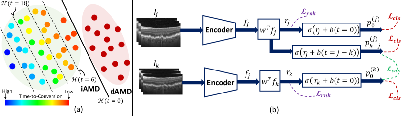
Figure 1: (a) Illustration of the proposed method. (b) Proposed Training pipeline employs the same ConvNeXt-Tiny Encoder in both branches with shared weights.

Proposed Disease Progression Formulation: The proposed method combines two distinct approaches of forecasting disease progression. First, we model the conversion time as a random variable $T^{*}$ with corresponding Cumulative Distribution Function (CDF) function $p(t|\vec{I})=P(T^{*}\leq t|\vec{I})$ and $\vec{I}\in\mathcal{I}$ is a space of all possible images. Second, for each $\vec{I}$ with conversion time $T$ we assign a risk score $r:\mathcal{I}\rightarrow\mathbb{R}$ such that $\forall\vec{I_{1}},\vec{I_{2}}\in\mathcal{I},T_{1}\leq T_{2}:r(\vec{I_{1}})\geq r(\vec{I_{2}})$. The first interpretation estimates a patient’s $t$-year survival likelihood (CDF) while the second can stratify a population into low, medium, and high risk groups by thresholding the risk score. Our proposed formulation illustrated in Fig. 1(a) combines both of these approaches.

A CNN encoder maps each scan $\vec{I}$ to a point in the feature embedding space (represented as dots in Fig. 1(a)). Then, these features are fed into a linear iAMD vs. dAMD stage classifier with weights $\vec{w}$ and a scalar bias $\beta$. Notably, the $\vec{w}$ vector is normal to the classifier’s decision hyperplane $H$ such that $\forall f\in H:{\vec{w}}^{\mkern-4.0mu\top}\vec{f}+\beta=0$. For a given $\vec{f}$, its shortest signed distance perpendicular to $H$ is proportional(scaled by a factor of $||w||$) to ${\vec{w}}^{\mkern-4.0mu\top}.\vec{f}+\beta$. The iAMD samples lie on the negative half-space (${\vec{w}}^{\mkern-4.0mu\top}.\vec{f}+\beta<0$) with negative signed distances from $H$.

Risk score based on distance from $H$: We introduce a temporal ordering among the iAMD samples with a ranking loss $\mathcal{L}_{rnk}$ (details discussed below), such that the distance of each sample from $H$ is inversely related to its conversion time $T^{*}$. This is illustrated in Fig. 1(a) by color grading each iAMD sample from red to blue in increasing order of $T^{*}$. Rank ordering serves multiple objectives. First, it acts as a regularizer for learning a semantically meaningful feature space with a better chance of generalization when trained on limited labeled data. Second, the signed distance from $H$ can be used as a risk score

$$r={\vec{w}}^{\mkern-4.0mu\top}\vec{f},$$ (1)

such that the higher the $r$, the closer it is to conversion. $\beta$ being constant across all samples can be ignored for ranking. Risk score is further calibrated in a post-processing step to normalize to $[0,1]$. After training, $r$ is obtained for all scans in the validation set and a bicubic interpolation is learned to map the k-th percentile of $r$ values to $k/100$ in increments of 10 percentiles.

Modeling CDF with a family of hyperplanes parallel to $H$: We propose a novel continuous-time modeling of the CDF to leverage the temporal ranking in the feature space. Predicting $p_{t}$ involves learning a separate linear binary classifier for each time-interval $t$ to predict if $\vec{I}$ will convert within $t$. $t$ is normalized such that $0-3$ years is linearly mapped in the range $[0,1]$. We extend our formulation by considering a continuous family of separating hyperplanes $\mathcal{H}(t)$ parallel to $H$, each predicting the conversion within $t$ (depicted with dashed lines in Fig. 1(a)). All hyperplanes in $\mathcal{H}(t)$ share the normal vector $\vec{w}$ but employ a different bias $b(t)$, parameterized as a monotonic function of $t$. Thus,

$$p_{t}(\vec{I})=\sigma\left({\vec{w}}^{\mkern-4.0mu\top}\vec{f}+b(t)\right)=\sigma\left(r+b(t)\right),$$ (2)

where $\sigma(.)$ is the sigmoid function. We reformulated bias $b(t)$ as an affine transformation $b(t)=\alpha\cdot t+\beta$, where $\alpha$ and $\beta$ are scalar learnable parameters of our model. The hyperplane $H$ for iAMD vs dAMD stage classification is a member of this family, $H=\mathcal{H}(t=0)$. Thus, $p_{0}=\sigma\left({\vec{w}}^{\mkern-4.0mu\top}\vec{f}+b(0)\right)=\sigma\left({\vec{w}}^{\mkern-4.0mu\top}\vec{f}+\beta\right)$ is the probability that the current input scan $\vec{I}$ has already converted to the dAMD.

Training Pipeline: We consider a Siamese architecture (Fig. 1(b)) during training to leverage the availability of longitudinal images by considering image-pairs from different eyes in each training batch. Each random image-pair $(\vec{I}_{j},\vec{I}_{k})$ are two OCT scans of the same eye, acquired at different patient visits at time-points $j$ and $k$. $\vec{I}_{j}$ precedes $\vec{I}_{k}$ (i.e., $j<k$) with a time-interval of (j-k) between them. Both $\vec{I}_{j},\vec{I}_{k}$ are fed to an Encoder (ConvNeXt-Tiny initialized with ImageNet pretrained weights [8]), to obtain the features $\vec{f}_{j},\vec{f}_{k}$ respectively. Their risk scores $r_{j}$ and $r_{k}$ are obtained using Eq. 1 and the probabilities $p_{0}^{(j)}$ and $p_{0}^{(k)}$ that $\vec{I}_{j}$ and $\vec{I}_{k}$ have already converted to dAMD are computed using Eq. 2. Additionally, we compute the probability of $\vec{I}_{j}$ to convert to dAMD within the next (k-j) time-interval as $p_{k-j}^{(j)}=\sigma\left(r_{j}+b(k-j)\right)$. Thus, while $p_{j}^{(0)}$ and $p_{k}^{(0)}$ essentially perform an iAMD vs. dAMD stage classification for the input scan, $p_{k-j}^{(j)}$ forecasts the conversion probability for a future time-point $k$, directly from a previous visit $\vec{I}_{j}$ without accessing $\vec{I}_{k}$.

Loss Functions: Following survival analysis, the Ground Truth (GT) labels for each scan $\vec{I}_{j}$ is denoted by the tuple $\left(T_{j},E_{j}\right)$. If the binary event indicator $E_{j}=1$, then the eye to which $\vec{I}_{j}$ belongs, converts to dAMD after a time-interval $T_{j}$ from the current visit. $E_{j}=0$ indicates that the eye did not convert within the monitoring period in which case $T_{j}$ represents time duration from the current to the last visit in the study after which the eye is censored.

Classification Loss $\mathcal{L}_{cls}$: The GT for iAMD vs dAMD classification for an eye at a time-point $j$ is given by $y_{j}=1$ if it has already converted, i.e., $E_{j}=1$ and $T_{j}<=0$, otherwise $y_{j}=0$. The binary cross entropy loss $\mathcal{L}_{bce}(.)$ is used to define the classification loss as $\mathcal{L}_{cls}=\mathcal{L}_{bce}(y_{j},p^{(j)}_{0})+\mathcal{L}_{bce}(y_{k},p^{(k)}_{0})+\mathcal{L}_{bce}(y_{k},p^{(j)}_{k-j})$.

Intra-Subject Consistency Loss $\mathcal{L}_{cns}$: For a given eye, the conversion probability at a time-point $k$ predicted from the scan acquired at time $k$($p_{0}^{(k)}$) should be consistent with the probability forecast for $k$, using a previous scan from time-point $j$ ($p_{k-j}^{(j)}$). This is ensured with the consistency loss $\mathcal{L}_{cns}=\mathcal{L}_{bce}(p_{0}^{(k)},p_{k-j}^{(j)})$.

Temporal Ranking Loss $\mathcal{L}_{rnk}$: We consider all possible image-pairs $(\vec{I}_{m},\vec{I}_{n})$ in a training batch (including pair of scans coming from different eyes). $\mathcal{L}_{rnk}$ solves a logistic regression task using the difference in risks $(r_{m}-r_{n})$ as input to a linear classifier to predict the probability $p_{m<n}$ of $\vec{I}_{m}$ converting before $\vec{I}_{n}$ as $\mathcal{L}_{rnk}=-\frac{1}{|S_{m<n}|+|S_{m>n}|}.\left[\sum_{S_{m}<n}log\left(p_{m<n}\right)+\sum_{S_{m>n}}log\left(1-p_{m<n}\right)\right]$, where $S_{m<n}$ represents a subset of all possible image-pairs in a training batch where $I_{m}$ converts before $I_{n}$ for which ideally, $p_{m<n}\approx 1$. Similarly, $S_{m>n}$ contains image-pairs where $\vec{I}_{m}$ converts after $\vec{I}_{n}$ and ideally, $p_{m<n}\approx 0$. The set $S_{m<n}$ comprises image-pairs for which $\{(T_{m}<T_{n})$ $\&$ $(E_{m}=1$ or $\vec{I_{m}}$, $\vec{I_{n}}$ belong to the same eye)$\}$. AMD progression is irreversible and the retinal tissue damage only accumulates with time. Therefore, even for cases where $E=0$ and the actual conversion time is unknown, the risk score of a scan from a later visit $\vec{I}_{m}$( with a smaller time duration $T_{m}$ to the last visit) should always be higher than a former visit $\vec{I}_{n}$ ($T_{n}>T_{m}$) of the same eye. Similarly, $S_{m>n}$ is defined as pairs where $\{(T_{m}>T_{n})$ $\&$ $(E_{n}=1$ or $\vec{I_{m}}$, $\vec{I_{n}}$ belong to the same eye)$\}$.

Thus, the total loss is defined as $\mathcal{L}=\mathcal{L}_{cls}+\mathcal{L}_{cns}+\mathcal{L}_{rnk}$ with equal weights given to each term. While a Siamese two-branch architecture is employed during training, only a single branch is employed during inference. The proposed method employs a single visit’s scan $\vec{I}$ as input to predict $r$ (see Eq. 2) and the probability of conversion $p_{t}$ within a given future time-interval $t$ (see Eq. 1).

Unsupervised Fine-tuning on External Datasets: We adapt our training losses to facilitate unsupervised fine-tuning with unlabeled data. $\mathcal{L}_{cls}$ requires GT labels and, therefore, is not used. The unsupervised loss $\mathcal{L}_{cns}$ leverages the consistency in the predictions from the two branches of the Siamese architecture and is retained unmodified. $\mathcal{L}_{rnk}$ is adjusted in how $\vec{I_{m},\vec{I}_{n}}$ pairs are constructed within each training batch. In the absence of conversion time labels, risk scores of scans across the batch samples cannot be compared. Only the intra-subject sample pairs $\vec{I_{j},\vec{I}_{k}}$ are utilized, as they should still be be ranked as $r_{k}>r_{j}$ for time-points $k>j$ as AMD being degenerative cannot regress with time.

Implementation Details: Our method was implemented in Python 3.8, PyTorch 2.0.0 (code available at https://github.com/arunava555/Forecast_parallel_hyperplanes ). The training comprised 200 epochs (with 300 batch updates per epoch, batch size of 16), employing the AdamW optimizer [9] with a cyclic learning rate [17] varying between $10^{-6}$ to $10^{-4}$. Each training batch was constructed with random image-pairs $(\vec{I}_{j},\vec{I}_{k})$ with a time-interval of 0-3 years between them, ensuring that all $\vec{I}_{j}$ were in the iAMD stage, while half of the $\vec{I}_{k}$ in each batch were in the dAMD stage (through oversampling). Three consecutive B-scans (slices) out of the 5 central B-scans in the OCT volumes were randomly extracted and input to Encoder in place of the three RGB color channels. Data augmentations included random translations, horizontal flip, random crop-resize, Gaussian noise, random in-painting and random intensity transformations. During inference, for each scan, three sets of 3-channel input images were formed from the 5 central OCT slices, each containing the central slice in the left, middle or right channel. An average of their predictions were used for all experiments (including the benchmark methods for comparison).

3 Experiments and Results

Datasets: We comprehensively evaluated our method on Dataset-1 collected at the Department of Ophthalmology, Medical University of Vienna, comprising 3,534 OCT scans from 235 eyes (40 converters and 195 censored) acquired with a Spectralis OCT scanner at a resolution of 49 B-scans (slices), each with a $512-1024\times 49$ px. For converter eyes, labels for each scan were computed by measuring the time interval between its acquisition and the first conversion visit. We considered an additional independent, external real-world dataset, Dataset-2, collected from two different sites (University Hospital Southampton and Moorfields Eye Hospital) from the PINNACLE consortium [18]. It comprises a randomly divided training set of 254 eyes (2428 scans) with 49 converters; a validation set of 127 eyes (1073 scans) with 26 converters; and a test set of 254 eyes (2305 scans) with 49 converters. All scans were acquired with Topcon scanners at a resolution of 128 B-scans with a $885\times 512$ px. The scans from Dataset-1 and Dataset-2 exhibit large image domain shift due to different imaging scanners.

Table 1: Ablation and Comparison with state-of-the art on Dataset-1.

	AUROC				Balanced Accuracy
	6	12		24	6	12		24	CcI
$\mathcal{L}_{cls}$	$0.816\pm 0.05$	$0.792\pm 0.06$		$0.771\pm 0.06$	$0.802\pm 0.04$	$0.769\pm 0.05$		$0.744\pm 0.04$	$0.740\pm 0.06$
$\mathcal{L}_{cls}+\mathcal{L}_{rnk}$	$0.823\pm 0.07$	$0.805\pm 0.04$		$0.772\pm 0.02$	$\mathbf{0.816\pm 0.05}$	$0.772\pm 0.02$		$0.742\pm 0.02$	$0.752\pm 0.03$
Proposed	$\mathbf{0.825\pm 0.09}$	$\mathbf{0.828\pm 0.07}$		$\mathbf{0.809\pm 0.06}$	$0.813\pm 0.06$	$\mathbf{0.798\pm 0.05}$		$\mathbf{0.770\pm 0.06}$	$\mathbf{0.783\pm 0.06}$
Cens. CE [21]	$0.787\pm 0.06$	$0.779\pm 0.06$		$0.789\pm 0.04$	$0.764\pm 0.05$	$0.739\pm 0.04$		$0.741\pm 0.02$	$0.767\pm 0.04$
Logis. Hazard [12]	$0.787\pm 0.06$	$0.787\pm 0.04$		$0.797\pm 0.03$	$0.780\pm 0.06$	$0.766\pm 0.03$		$0.755\pm 0.04$	$0.769\pm 0.04$
DeepSurv [4]	$0.755\pm 0.13$	$0.735\pm 0.12$		$0.728\pm 0.12$	$0.734\pm 0.12$	$0.702\pm 0.10$		$0.679\pm 0.09$	$0.768\pm 0.04$
SODEN [19]	$0.673\pm 0.09$	$0.707\pm 0.05$		$0.721\pm 0.05$	$0.676\pm 0.05$	$0.691\pm 0.03$		$0.698\pm 0.04$	$0.710\pm 0.05$

Results on Dataset-1: An eye-level stratified five-fold cross-validation was performed. In each fold, the training set was further sub-divided to use $20\%$ as a validation set. The test set in each fold comprised 667-707 scans from 47 eyes with 8 converters. While the converted dAMD scans were also used during training, they were removed from the test set to focus on forecasting conversions from iAMD images alone. The Area under the ROC curve (AUROC) and Balanced Accuracy (B.Acc) were reported for predicting conversion within the next $6$, $12$ and $24$ months (Table 1). Concordance Index (CcI) was used to evaluate the risk scores $r$ on their ability to provide a reliable ranking of the conversion time.

Ablation Experiments show that training with $\mathcal{L}_{cls}$ and $\mathcal{L}_{rnk}$ (row 2) leads to a marginal improvement over training with $\mathcal{L}_{cls}$ alone (row 1) across all time-points in terms of AUROC, B.Acc(except $t=24$) as well as CcI (0.740 to 0.752) demonstrating the positive impact of imposing rank ordering. The proposed method additionally incorporates $\mathcal{L}_{cns}$ (over row 2) which led to a considerable performance improvement in terms of CcI (0.752 to 0.783) as well as the AUROC and B.Acc across all $t$ (except for B.Acc at $t=6$). Overall, the results demonstrate the value of using all loss terms.

Comparison with State-of-the-art was performed against popular survival analysis techniques in rows 3-7. These include discrete survival analysis methods utilizing censored cross-entropy loss (Cens. CE) from [21] and a logistic hazard model [12], both employing discrete 6-month time-windows for predicting conversion. Additionally, DeepSurv [4] extends the CoxPH model using Deep Learning, while SODEN [19] is a Neural-ODE based approach, originally explored for tabular data. These methods were implemented with the ConvNeXt-Tiny encoder by modifying the classification layers and losses. All of these methods do not employ intra-subject regularization, hence require training a single branch network. SODEN showed signs of overfitting with good performance on the validation set (to select the best-performing models) but led to a drop in performance on the test sets in all folds. The results demonstrate the superior performance of our proposed method, outperforming all other methods across all time-intervals.

Table 2: Performance (mean $\pm$ std. dev.) comparison between unsupervised (Unsup.-F) and Supervised (Sup.-F) Fine-tuning on Dataset-2.

	AUROC				Balanced Accuracy
	6	12		24	6	12		24	CcI
Cross-Test	$0.748\pm 0.04$	$0.764\pm 0.05$		$0.758\pm 0.05$	$0.702\pm 0.03$	$0.712\pm 0.04$		$0.707\pm 0.04$	$0.756\pm 0.04$
Finetuning with $25\%$ training data
Unsup.-F	$0.823\pm 0.01$	$0.837\pm 0.01$		$0.826\pm 0.01$	$0.774\pm 0.01$	$0.783\pm 0.02$		$0.764\pm 0.01$	$0.818\pm 0.01$
Sup.-F	$0.824\pm 0.02$	$0.837\pm 0.01$		$0.825\pm 0.01$	$0.766\pm 0.02$	$0.776\pm 0.01$		$0.766\pm 0.01$	$0.816\pm 0.02$
Finetuning with $100\%$ training data
Unsup.-F	$0.837\pm 0.01$	$0.849\pm 0.01$		$0.834\pm 0.01$	$0.8\pm 0.01$	$0.809\pm 0.01$		$0.775\pm 0.01$	$0.828\pm 0.01$
Sup.-F	$0.845\pm 0.01$	$0.853\pm 0.01$		$0.845\pm 0.01$	$0.786\pm 0.02$	$0.793\pm 0.02$		$0.773\pm 0.01$	$0.831\pm 0.01$

Results on Dataset-2: We analyzed the effect of adapting our models pre-trained on Dataset-1, to Dataset-2 through unsupervised fine-tuning (Table 2). While the validation and test sets remained fixed across all experiments, the training set size for fine-tuning was varied by considering the entire ($100\%$) and a $25\%$ subset (Supplemental Table 4 reports $50\%$ and $75\%$). Each experiment was repeated five times, each time using a different model weight for initialization trained on each of the five-folds in Dataset-1. A different randomly selected subset of the training data of Dataset-2 was employed each time except when fine-tuning on the entire ($100\%$) training dataset. Cross-testing performance in row 1, directly applied the models trained on Dataset-1 without fine-tuning. A moderate drop in performance was observed in comparison to fine-tuned models, which is expected due to the image domain shift across scanners.

Unsupervised Fine-tuning (Unsup.-F) was performed by leveraging the inter-dependencies between longitudinal intra-subject image-pairs without using the GT training conversion-time labels. A drastic performance improvement was observed over cross-testing both in AUROC and B.Acc. across all time-intervals. The CcI improved from $0.756$ to $0.818$ by just utilizing $25\%$ of the training data (row 1 vs 2). The unsupervised fine-tuning performance further improved (row 2 vs 4) by utilizing the entire training dataset in an unsupervised manner. Fully supervised fine-tuning (Sup.-F) with GT conversion labels serve as an upper limit on fine-tuning performance. Interestingly, the performance gap between Unsup.-F and Sup-F was not significant in the small training data-regime (row 2 vs 3) with an almost same mean AUROC across $6$, $12$ and $18$ months, while Unsup.-F surpassed Sup.-F in terms of B.Acc at $t=6,12$ and CcI (0.818 vs. 0.816). However, this trend reverses when the entire training dataset was utilized (row 4-5) in terms of AUROC, with the Unsup.-F still giving competitive performance in terms of B.Acc and CcI (0.828 for Unsup.-F compared to 0.831 for Sup.-F). Fig. 2(a) displays Kaplan-Meier survival curves for risk groups identified by thresholding $r$ from a model trained on $25\%$ of Dataset-2’s training data with Unsup.-F. The curves are distinctly separated, affirming $r$’s efficacy in stratifying risk. Fig. 2(b) illustrates the U-map visualization of the model’s feature space, transitioning smoothly from red (short conversion time) to blue (long conversion time) along the manifold. GradCam maps in Fig. 2(c) reveal that the trained models attend to irregularities around drusen, known markers of AMD.

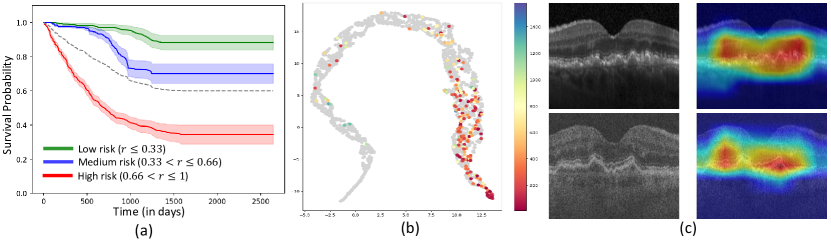
Figure 2: (a) Kaplan-Meier Curves. (b) U-Map feature space visualization of the test set of Dataset-2. (c) An example of domain-shift between scans from Dataset-1(top) and Dataset-2(bottom) along with GradCam saliency maps highlighting drusen.

4 Conclusion

We proposed a novel framework to jointly predict a risk score and predict the CDF of conversion at given continuous time-intervals. The risk score, based on the signed distance of a sample from a decision hyperplane $H$ separating iAMD and dAMD samples, incorporates a ranking loss to to ensure that samples closest to $H$ have the shortest conversion time and vice versa. This temporal ordering in the feature space is further utilized to model the CDF, predicting conversion probabilities at arbitrary future time intervals using a family of hyperplanes parallel to $H$. We also enforce dependencies between intra-subject longitudinal image pairs to regularize the feature space, facilitating unsupervised fine-tuning on new datasets. Our method outperforms several popular survival analysis methods, demonstrating its effectiveness. In addition, unsupervised fine-tuning significantly improved cross-testing performance across datasets particularly with limited training data availability. This approach allows for model adaptation across datasets with significant domain shifts due to inter-scanner variability without the need for manual annotation of training labels. Future work could include evaluating our method on public datasets for related tasks like Alzheimer’s disease progression from brain MRI and incorporating Longitudinal-Mixup [23] in our training to improve performance.

4.0.1 Acknowledgements

This research was funded in part by the Austrian Science Fund (FWF) [10.55776/FG9], and Wellcome Trust Collaborative Award Ref. 210572/Z/18/Z.

Appendix 0.A Supplementary Material

Table 3: Performance at Eye-level on Dataset-1 achieved through bootstrapping with $1000$ resamplings. Each resampling involves randomly selecting one scan per eye from a single visit. Mean and standard deviation are computed across $5$ folds $\times$ $1000$ bootstrap samples.

	AUROC				Balanced Accuracy
	6	12		24	6	12		24	CcI
Proposed	$\mathbf{0.835\pm 0.16}$	$\mathbf{0.826\pm 0.11}$		$\mathbf{0.798\pm 0.08}$	$\mathbf{0.824\pm 0.10}$	$\mathbf{0.794\pm 0.09}$		$\mathbf{0.774\pm 0.08}$	$\mathbf{0.780\pm 0.06}$
Cens. CE [21]	$0.775\pm 0.14$	$0.772\pm 0.13$		$0.790\pm 0.08$	$0.804\pm 0.11$	$0.756\pm 0.11$		$0.746\pm 0.06$	$0.762\pm 0.06$
Logis. Hazard [12]	$0.769\pm 0.19$	$0.768\pm 0.12$		$0.786\pm 0.08$	$0.792\pm 0.14$	$0.760\pm 0.11$		$0.766\pm 0.08$	$0.749\pm 0.08$
DeepSurv [4]	$0.769\pm 0.18$	$0.710\pm 0.16$		$0.723\pm 0.14$	$0.749\pm 0.17$	$0.689\pm 0.12$		$0.686\pm 0.12$	$0.752\pm 0.07$
SODEN [19]	$0.675\pm 0.24$	$0.674\pm 0.17$		$0.698\pm 0.11$	$0.711\pm 0.19$	$0.671\pm 0.14$		$0.693\pm 0.10$	$0.673\pm 0.09$

Table 4: Performance (mean $\pm$ std. dev.) comparison between unsupervised (Unsup.-F) and Supervised (Sup.-F) Fine-tuning on Dataset-2.

	AUROC				Balanced Accuracy
	6	12		24	6	12		24	CcI
Finetuning with $50\%$ training data
Unsup.-F	$0.829\pm 0.01$	$0.843\pm 0.01$		$0.829\pm 0.01$	$0.790\pm 0.01$	$0.801\pm 0.01$		$0.772\pm 0.01$	$0.822\pm 0.01$
Sup.-F	$0.835\pm 0.02$	$0.847\pm 0.01$		$0.839\pm 0.01$	$0.788\pm 0.01$	$0.795\pm 0.01$		$0.772\pm 0.01$	$0.825\pm 0.01$
Finetuning with $75\%$ training data
Unsup-F	$0.833\pm 0.01$	$0.851\pm 0.01$		$0.834\pm 0.01$	$0.785\pm 0.01$	$0.807\pm 0.01$		$0.773\pm 0.01$	$0.831\pm 0.01$
Sup-F	$0.844\pm 0.01$	$0.856\pm 0.01$		$0.843\pm 0.01$	$0.777\pm 0.01$	$0.789\pm 0.01$		$0.77\pm 0.01$	$0.833\pm 0.01$

Table 5: Eye-level Performance on Dataset-2 computed through bootstrapping with $1000$ resamplings. Each resampling involves randomly selecting one scan per eye from a single visit. Mean and standard deviation are computed across $5$ folds $\times$ $1000$ bootstrap samples. Unsupervised(Unsup.-F) and Supervised(Sup.-F) Fine-tuning are compared.

	AUROC				Balanced Accuracy
	6	12		24	6	12		24	CcI
Cross-Test	$0.749\pm 0.06$	$0.762\pm 0.06$		$0.753\pm 0.06$	$0.716\pm 0.05$	$0.719\pm 0.05$		$0.703\pm 0.05$	$0.739\pm 0.06$
Finetuning with $25\%$ training data
Unsup-F	$0.816\pm 0.03$	$0.832\pm 0.02$		$0.823\pm 0.02$	$0.758\pm 0.03$	$0.775\pm 0.03$		$0.763\pm 0.02$	$0.813\pm 0.02$
Sup-F	$0.812\pm 0.03$	$0.833\pm 0.02$		$0.821\pm 0.02$	$0.762\pm 0.04$	$0.776\pm 0.03$		$0.76\pm 0.02$	$0.81\pm 0.02$
Finetuning with $50\%$ training data
Unsup-F	$0.821\pm 0.03$	$0.835\pm 0.02$		$0.824\pm 0.02$	$0.77\pm 0.03$	$0.789\pm 0.02$		$0.771\pm 0.02$	$0.816\pm 0.02$
Sup-F	$0.824\pm 0.03$	$0.842\pm 0.02$		$0.836\pm 0.02$	$0.775\pm 0.03$	$0.79\pm 0.02$		$0.774\pm 0.02$	$0.818\pm 0.02$
Finetuning with $75\%$ training data
Unsup-F	$0.827\pm 0.03$	$0.843\pm 0.02$		$0.827\pm 0.02$	$0.77\pm 0.03$	$0.791\pm 0.02$		$0.769\pm 0.02$	$0.824\pm 0.01$
Sup-F	$0.83\pm 0.02$	$0.85\pm 0.02$		$0.839\pm 0.02$	$0.771\pm 0.03$	$0.792\pm 0.02$		$0.771\pm 0.02$	$0.827\pm 0.01$
Finetuning with $100\%$ training data
Unsup-F	$0.838\pm 0.03$	$0.847\pm 0.02$		$0.834\pm 0.02$	$0.788\pm 0.03$	$0.796\pm 0.02$		$0.772\pm 0.02$	$0.827\pm 0.01$
Sup-F	$0.83\pm 0.02$	$0.851\pm 0.02$		$0.844\pm 0.02$	$0.77\pm 0.03$	$0.796\pm 0.02$		$0.782\pm 0.02$	$0.828\pm 0.01$

References

- [1] Banerjee, I., de Sisternes, L., Hallak, J.A., Leng, T., Osborne, A., Rosenfeld, P.J., Gregori, G., Durbin, M., Rubin, D.: Prediction of age-related macular degeneration disease using a sequential deep learning approach on longitudinal sd-oct imaging biomarkers. Scientific reports 10(1), 15434 (2020)
- [2] Emre, T., Chakravarty, A., Rivail, A., Riedl, S., Schmidt-Erfurth, U., Bogunović, H.: Tinc: Temporally informed non-contrastive learning for disease progression modeling in retinal oct volumes. In: International Conference on Medical Image Computing and Computer-Assisted Intervention. pp. 625–634. Springer (2022)
- [3] Heier, J.S., Lad, E.M., Holz, F.G., Rosenfeld, P.J., Guymer, R.H., Boyer, D., Grossi, F., Baumal, C.R., Korobelnik, J.F., Slakter, J.S., Waheed, N.K., Metlapally, R., Pearce, I., Steinle, N., Francone, A.A., Hu, A., Lally, D.R., Deschatelets, P., Francois, C., Bliss, C., Staurenghi, G., Monés, J., Singh, R.P., Ribeiro, R., Wykoff, C.C.: Pegcetacoplan for the treatment of geographic atrophy secondary to age-related macular degeneration (OAKS and DERBY): two multicentre, randomised, double-masked, sham-controlled, phase 3 trials. The Lancet 402(10411), 1434–1448 (oct 2023)
- [4] Katzman, J.L., Shaham, U., Cloninger, A., Bates, J., Jiang, T., Kluger, Y.: Deepsurv: personalized treatment recommender system using a cox proportional hazards deep neural network. BMC medical research methodology 18(1), 1–12 (2018)
- [5] Khanani, A.M., Patel, S.S., Staurenghi, G., Tadayoni, R., Danzig, C.J., Eichenbaum, D.A., Hsu, J., Wykoff, C.C., Heier, J.S., Lally, D.R., Monés, J., Nielsen, J.S., Sheth, V.S., Kaiser, P.K., Clark, J., Zhu, L., Patel, H., Tang, J., Desai, D., Jaffe, G.J.: Efficacy and safety of avacincaptad pegol in patients with geographic atrophy (GATHER2): 12-month results from a randomised, double-masked, phase 3 trial. The Lancet 402(10411), 1449–1458 (oct 2023)
- [6] Lachinov, D., Chakravarty, A., Grechenig, C., Schmidt-Erfurth, U., Bogunović, H.: Learning spatio-temporal model of disease progression with neuralodes from longitudinal volumetric data. IEEE Transactions on Medical Imaging (2023)
- [7] Lad, E.M., Sleiman, K., Banks, D.L., Hariharan, S., Clemons, T., Herrmann, R., Dauletbekov, D., Giani, A., Chong, V., Chew, E.Y., et al.: Machine learning oct predictors of progression from intermediate age-related macular degeneration to geographic atrophy and vision loss. Ophthalmology Science 2(2), 100160 (2022)
- [8] Liu, Z., Mao, H., Wu, C.Y., Feichtenhofer, C., Darrell, T., Xie, S.: A convnet for the 2020s. In: Proceedings of the IEEE/CVF conference on computer vision and pattern recognition. pp. 11976–11986 (2022)
- [9] Loshchilov, I., Hutter, F.: Decoupled weight decay regularization. In: International Conference on Learning Representations (2018)
- [10] Nyúl, L.G., Udupa, J.K., Zhang, X.: New variants of a method of mri scale standardization. IEEE transactions on medical imaging 19(2), 143–150 (2000)
- [11] Rivail, A., Schmidt-Erfurth, U., Vogl, W.D., Waldstein, S.M., Riedl, S., Grechenig, C., Wu, Z., Bogunovic, H.: Modeling disease progression in retinal octs with longitudinal self-supervised learning. In: Predictive Intelligence in Medicine: Second International Workshop, PRIME 2019, Held in Conjunction with MICCAI 2019, Shenzhen, China, October 13, 2019, Proceedings 2. pp. 44–52. Springer (2019)
- [12] Rivail, A., Vogl, W.D., Riedl, S., Grechenig, C., Coulibaly, L.M., Reiter, G.S., Guymer, R.H., Wu, Z., Schmidt-Erfurth, U., Bogunović, H.: Deep survival modeling of longitudinal retinal oct volumes for predicting the onset of atrophy in patients with intermediate amd. Biomedical Optics Express 14(6), 2449–2464 (2023)
- [13] Russakoff, D.B., Lamin, A., Oakley, J.D., Dubis, A.M., Sivaprasad, S.: Deep learning for prediction of amd progression: a pilot study. Investigative ophthalmology & visual science 60(2), 712–722 (2019)
- [14] Schmidt-Erfurth, U., Waldstein, S.M., Klimscha, S., Sadeghipour, A., Hu, X., Gerendas, B.S., Osborne, A., Bogunović, H.: Prediction of individual disease conversion in early amd using artificial intelligence. Investigative ophthalmology & visual science 59(8), 3199–3208 (2018)
- [15] de Sisternes, L., Simon, N., Tibshirani, R., Leng, T., Rubin, D.L.: Quantitative sd-oct imaging biomarkers as indicators of age-related macular degeneration progression. Investigative ophthalmology & visual science 55(11), 7093–7103 (2014)
- [16] Sleiman, K., Veerappan, M., Winter, K.P., McCall, M.N., Yiu, G., Farsiu, S., Chew, E.Y., Clemons, T., Toth, C.A., Wong, W., et al.: Optical coherence tomography predictors of risk for progression to non-neovascular atrophic age-related macular degeneration. Ophthalmology 124(12), 1764–1777 (2017)
- [17] Smith, L.N.: Cyclical learning rates for training neural networks. In: 2017 IEEE winter conference on applications of computer vision (WACV). pp. 464–472. IEEE (2017)
- [18] Sutton, J., Menten, M.J., Riedl, S., Bogunović, H., Leingang, O., Anders, P., Hagag, A.M., Waldstein, S., Wilson, A., Cree, A.J., et al.: Developing and validating a multivariable prediction model which predicts progression of intermediate to late age-related macular degeneration—the pinnacle trial protocol. Eye 37(6), 1275–1283 (2023)
- [19] Tang, W., Ma, J., Mei, Q., Zhu, J.: Soden: A scalable continuous-time survival model through ordinary differential equation networks. The Journal of Machine Learning Research 23(1), 1516–1544 (2022)
- [20] Wong, W.L., Su, X., Li, X., Cheung, C.M.G., Klein, R., Cheng, C.Y., Wong, T.Y.: Global prevalence of age-related macular degeneration and disease burden projection for 2020 and 2040: a systematic review and meta-analysis. The Lancet Global Health 2(2), e106–e116 (2014)
- [21] Wulczyn, E., Steiner, D.F., Xu, Z., Sadhwani, A., Wang, H., Flament-Auvigne, I., Mermel, C.H., Chen, P.H.C., Liu, Y., Stumpe, M.C.: Deep learning-based survival prediction for multiple cancer types using histopathology images. PloS one 15(6), e0233678 (2020)
- [22] Yim, J., Chopra, R., Spitz, T., Winkens, J., Obika, A., Kelly, C., Askham, H., Lukic, M., Huemer, J., Fasler, K., et al.: Predicting conversion to wet age-related macular degeneration using deep learning. Nature Medicine 26(6), 892–899 (2020)
- [23] Zeghlache, R., Conze, P.H., Daho, M.E.H., Li, Y., Le Boité, H., Tadayoni, R., Massin, P., Cochener, B., Brahim, I., Quellec, G., et al.: Lmt: Longitudinal mixing training, a framework to predict disease progression from a single image. In: International Workshop on Machine Learning in Medical Imaging. pp. 22–32. Springer (2023)