Transient selection of competing order in frustrated spin Peierls systems
after a quench
Abstract
We study theoretically the dynamics of frustrated spin Peierls systems after a quench from the paramagnetic state to the magnetically ordered state. By constructing and numerical simulating a minimal model, we show that it can exhibit a transient non-collinear magnetic order before settling in the equilibrium collinear magnetic order. The transient magnetic order is selected by the phonon fluctuations originated from the initial state. Our results reveal a mechanism for controlling the phases of matter by exploiting incoherent, nonequilibrium fluctuations.
The rise of ultrafast optics and spectroscopies opens a non-thermal pathway for controlling the phases of matter [1, 2, 3]. For instance, pumping the system with a short laser pulse can quench one long range order in favor of the other in a system with multiple competing orders, which makes it possible to guide the system to a desired yet thermodynamically metastable or even unstable state.
Frustrated magnets represent a prominent class of systems where competing orders appear naturally. Owing to the interplay between the lattice geometry and the exchange interactions, a frustrated magnet hosts distinct magnetic orders that are accidentally degenerate in energy in the mean field limit [4, 5]. Quantum/thermal fluctuations, or chemical/structural disorders may lift this accidental degeneracy through the order by disorder (ObD) mechanism [6, 7, 8], thereby stabilizing one magnetic order out of the many.
Among systems that host competing orders, frustrated magnets are unique in that their free energy landscape are strongly shaped by fluctuations. This trait opens new possibilities for controlling their phases out of the equilibrium. While the much explored Floquet engineering employs the coherent, periodic motion of normal modes [9, 10, 11, 12], less attension is paid to the utility of incoherent fluctuations. In this work, we reveal a mechanism by which transient magnetic orders emerge from such fluctuations in frustrated magnets coupled to soft phonons. After a quench induced by a laser pulse, the system can develop a thermodynamically unstable, competing magnetic order owing to the nonequilibrium phonon fluctuations, before it settles in the equilibrium one.
In equilibrium, a frustrated magnet exhibits the Peierls instability in the presence of spin-phonon coupling [13, 14, 15, 16]. The instability arises because the system releases the frustration by spontaneously distorting the lattice. When the spin-orbit coupling is weak, the spin-Peierls instability selects a collinear magnetic order among the degenerate magnetic orders.
We examine the evolution of the frustrated spin-Peierls systems after a quench from the paramagnetic state to the magnetically ordered state within the framework of time-dependent Ginzburg-Landau (TDGL) theory [17, 18, 19, 20, 21, 22]. In typical pump-probe experiments on magnets that use femtosecond laser pulses, the magnetic order melts rapidly, and then revives slowly as the system equilibrates [23, 24, 25, 3]. While the microscopic mechanisms for the melting and revival of magnetic order are complex, this process can be phenomenologically modeled by the TDGL formalism as a first approximation.
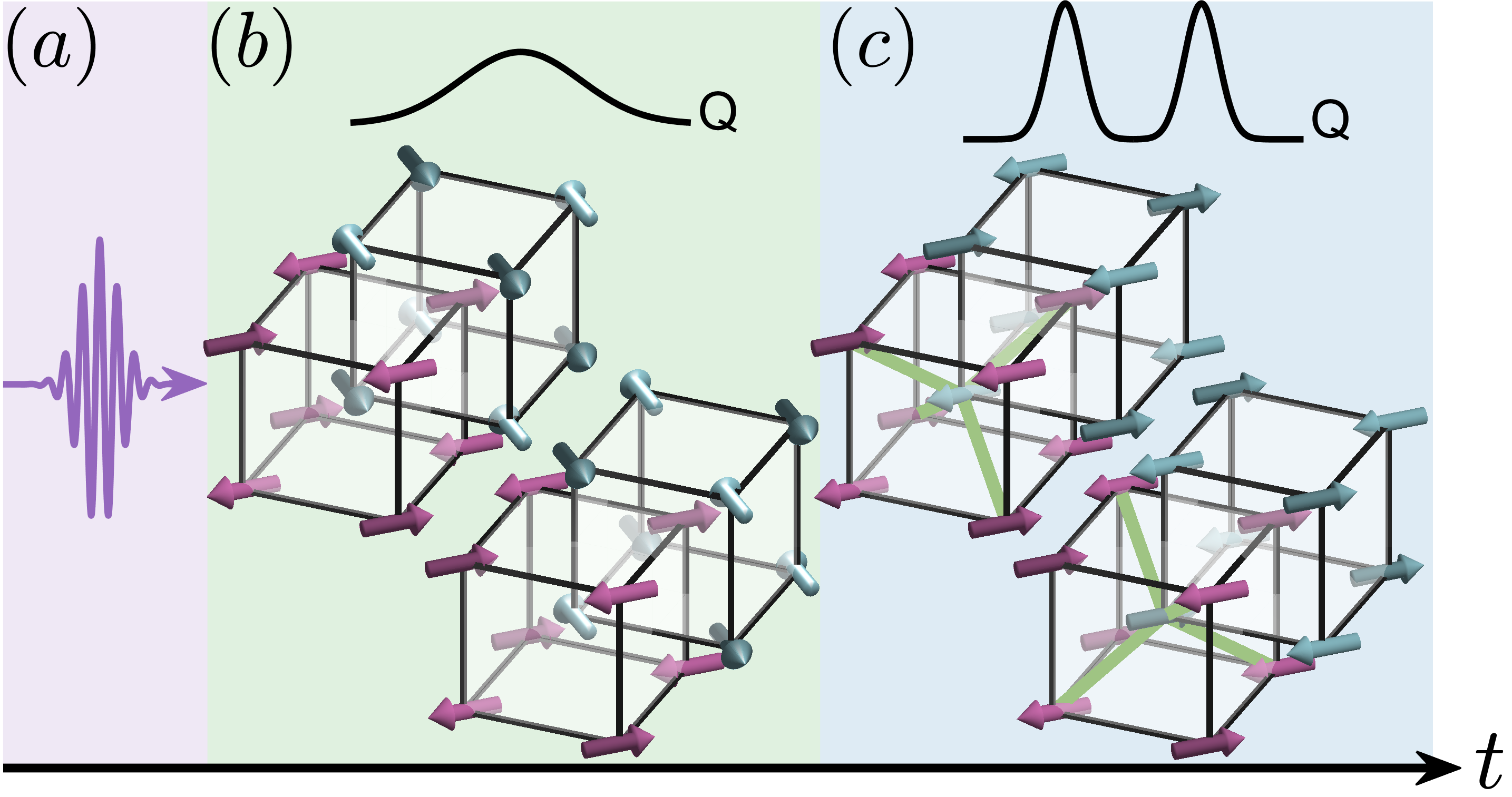
The phonon modes, described by their normal coordinates , are randomly distributed about in the initial paramagnetic state. Meanwhile, when the phonons are soft, their dynamics can be much slower than that of the spins. The phonons generate an effective, quenched disorder for the frustrated spins through the spin-phonon coupling at the initial stage of the time evolution. The quenched disorder, through the ObD mechanism, selects the non-collinear magnetic order [8] as opposed to the collinear magnetic order favored by the Peierls instability. As a result, the system must exhibit a tendency toward the thermally unstable non-collinear magnetic order before reverting to the collinear one (Fig. 1).
The dynamics of the system falls into the category of the phase ordering process [26, 27, 28]. As both the initial state and the equations of motion preserve all the symmetries, the system develop multiple domains instead of a single phase of the magnetic order in the thermodynamically limit. Particularly, the transient competing order manifests itself as the dominant correlations, rather than true long range order, in the early time, and survive as a subdominant short range order in the late time.
We expect that the above scenario is generic in that our arguments rely on the separation of time scales and the common features of the ObD physics. It can be viewed as a natural interpolation between two opposing order selection mechanisms in frustrated magnetism, namely the quenched disorder and the lattice distortion. In what follows, we construct a minimal model for frustrated spin-Peierls system, and demonstrate the transient magnetic order therein by a numerical simulation.
To set the stage, we consider an easy-plane antiferromagnet on the body-centered cubic (BCC) lattice with both nearest neighbor () and second neighbor () exchange interactions [29]. The BCC lattice comprises of two interpenetrating simple cubic sublattices, dubbed A and B, respectively. When , each sublattice hosts a Néel order, which are decoupled in the mean field limit (Fig. 1b&c).
Following a standard procedure [30], we write down the symmetry constrained Landau free energy, . describes the exchange interaction:
| (1a) | |||
| and describes the Néel order in sublattice A and B, respectively. are spin stiffness. It possesses two symmetries: The simultaneous rotation of and corresponds to the spin rotational symmetry. By contrast, the relative rotational symmetry reflects the accidental degeneracy due to the frustration. | |||
The spin-phonon part reads:
| (1b) |
Here, is the normal coordinate of an Einstein phonon. The spin-phonon coupling constant . Microscopically, it describes the modulation of the interactions by lattice distortion (Fig. 1c). is the elastic constant of phonons.
At equilibrium, minimizing yields the ground states, , , or , . These solutions describe the collinear magnetic orders, accompanied by a spontaneous distortion of the lattice (Fig. 1c).
We endow the system with model A dynamics [31]:
| (2) |
and are respectively the kinetic coefficients of the spins and the phonons. are three independent Gaussian white noises. Their second moments are determined by the fluctuation-dissipation theorem (FDT), , and , where is the bath temperature.
Before embarking on the analysis of the above model, we make a couple of extra steps to simplify it further. We define a pair of fields, , and . The equation of motion for and are then decoupled. is the order parameter corresponding to the spontaneous breaking of the spin rotational symmetry. parametrizes the continuous family of degenerate magnetic orders; the two Néel vectors are collinear when or , whereas they are orthogonal when . Since the focus is the selection of magnetic orders, we drop from now on.
We discretize the model on a cubic lattice for numerical simulation. After appropriate rescaling, we obtain:
| (3a) | |||
| with the free energy function: | |||
| (3b) | |||
is the dimensionless spin-phonon coupling constant. is lattice cutoff. . is the ratio between the characteristic relaxation time of the spins to that of the phonons. Crucially, when the phonons are soft (). The Gaussian white noises and obey the FDT: , and . is the dimensionless temperature.
Eq. (3) is the starting point of the ensuing analysis. We set the initial condition to be an uncorrelated state, where are drawn independently from a uniform distribution over , and from a Gaussian distribution with variance .
We begin with a qualitative analysis of Eq. (3) in a couple of limits. In the limit of , the phonons response immediately to the spins; therefore, we may set to its instantaneous equilibrium value, . Substituting by in the equation of motion for , we obtain an effective Landau energy for the spins, . The effective anisotropy term generated by the phonons lifts the accidental degeneracy, and favors the collinear magnetic orders, namely or . Therefore, the system exhibits the equilibrium magnetic order after the quench.
In the opposite limit of , are frozen to their initial states . The frozen phonons give rise to a random magnetic field in the direction, which favors the non-collinear states () [32, 33, 34]. To see this, we consider a single domain of size . Within the domain, the Landau energy has relaxed to its minimum. We write , where is the average orientation of the domain, and is the local variation due to random field. When , expanding to the second order in yields . Minimizing with respect to , and average over , we obtain . Here, is a numeric constant. Thus, the frozen phonons generate an effective anisotropy for , which favors , namely the states where the two Néel orders are orthogonal.
Having understood both limits, we consider the case with finite . For simplicity, we drop the white noise at the moment. Solving the equation of motion of , and substitute the solution into that of , we obtain:
| (4) |
The first summation on the right hand side is over all nearest neighbors. The second term is the random field due to the initial fluctuations. According to the preceding discussion, it generates an anisotropy that favors the non-collinear magnetic order. This anisotropy disappears after . Meanwhile, the third term is a retarded self-interaction mediated by phonons. For the dynamics over time scales , the Markov approximation reduces it to . This term selects the collinear order similar to the limit. We thus conclude that the non-collinear magnetic order develops over the time window , and gives way to the collinear magnetic order when .
We put this picture to test by numerically solving Eq. (3). We use a lattice subject to periodic boundary conditions, with the maximal size . We choose the representative model parameters and . The results do not show qualitative change so long as and is far below the ordering temperature. We solve the Langevin equation using the Euler method with time step . All results are obtained by averaging over 840 runs.
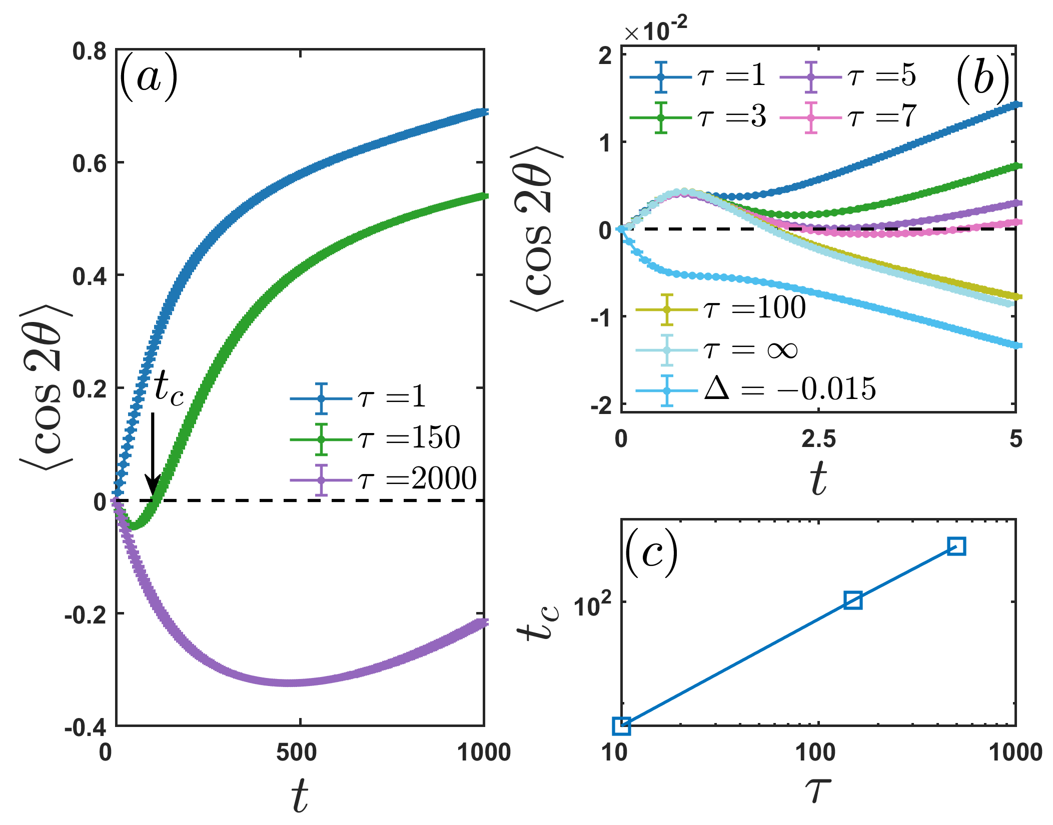
We characterize the magnetic order selection by the observable, . if , and if . Thus, this quantity measures the local anisotropy. Fig. 2a shows the numerically calculated as a function of time. For , it starts from 0 and increases in time, reflecting the building up of the local collinear magnetic order. By contrast, for , is negative within the simulated time window, indicating the selection of the local non-collinear magnetic order. Its magnitude reaches the maximum at . The non-monotonic behavior is due to the fact that the spin anisotropy generated by the phonon fluctuations is slowly decreasing in time.
More interesting is the case with , where changes sign at . This sign change is the manifestation of the change in the local magnetic order. In analogy with the spin reorientation transition in equilibrium [35], we dub the spin reorientation time.
It is natural to ask if observing the spin reorientation requires a minimum . To this end, we examine the early time behavior of (Fig. 2b). It starts out being positive at the initial stage for all values of . For , it remains positive throughout. On the other hand, for larger , it crosses to the negative side and then changes its sign again at . This sets a threshold at , below which the transient selection of the local non-collinear magnetic order does not occur.
The threshold stems from the fact that it takes a finite amount of time for the ObD phenomenon to establish. Even for , starts out being positive, and then becomes negative at . We heuristically understand this behavior as follows. The initial dynamics are dominated by the random field , which gives rise to a small but positive . The selection effect appears only after the exchange interaction generates spin correlations across a few lattice spacings. We stress that this behavior is a feature of the ObD physics; the sign change doesn’t occur if the random field is replaced by an anisotropy term (Fig. 2b).
Finally, for above the threshold, we find a linear scaling between the spin reorientation time and the phonon relaxation time (Fig. 2c), in agreement with the picture from the qualitative analysis.
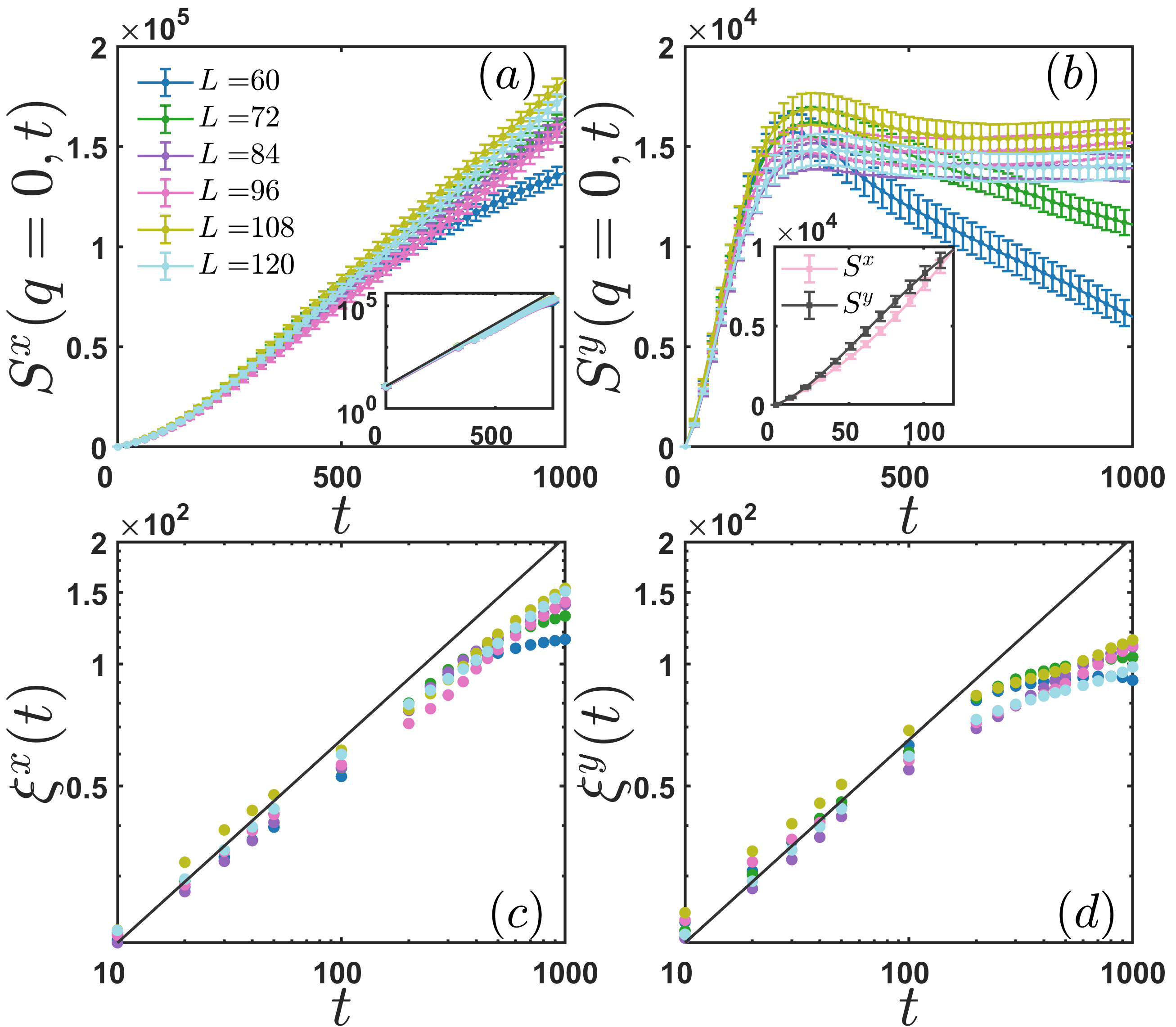
The observable is designed to probe local magnetic order. We now investigate the non-local spin correlations by measuring the time-dependent structure factor, . . , and . () probes the spatial correlation of the (non-)collinear magnetic order.
Fig. 3a shows , the height of the Bragg peak for the collinear magnetic order, as a function time. For prototypical phase ordering process such as that of the Ising model, the Bragg peak height exhibits a law, reflecting the domain growth [26]. The domain size grows as . As the height is proportional to the domain volume, it grows as . Here, exhibits an approximate law (Fig. 3a, inset).
We extract a correlation length from by measuring the half width at half maximum along the direction and using [30]. We observe a deviation from the growth law. At late time, the dynamics of the model is mapped to a three-dimensional XY model with easy axis anisotropy, which is in the same universality class as the Ising model. The deviation is likely due to uncertainties in measuring the correlation length at late time [30].
We then turn to the competing non-collinear magnetic order. Fig. 3b shows the evolution of . Crucially, is larger than that of at early time (Fig. 3b, inset), demonstrating that the non-collinear magnetic order is the dominant correlation in the transient regime. The time when the two are equal is slightly shorter but comparable to that of .
For finite system size, decreases to the equilibrium value at late time because the system is taken over by a single domain of the collinear magnetic order. This is not the case in the thermodynamic limit. As increases, the slope of the decrease is suppressed. The data therefore suggest saturates at late time. The anomalously large non-collinear spin correlation is the relic of the transient selection of the competing order.
The fact that the non-collinear magnetic order survives as a subdominant short-range order is mirrored in the correlation length (Fig. 3d). After an initial approximate growth, exhibits a kink near the spin reorientation time and continues to grow with much smaller slope.
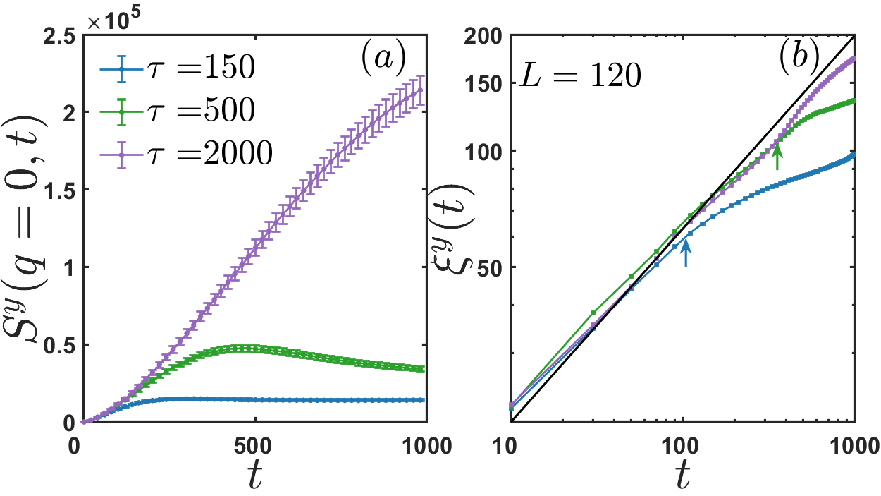
We now compare the evolution of non-collinear magnetic order for different phonon relaxation time ratios (Fig. 4). The overall magnitude of and increases with . The correlation length for and both show an initial approximate growth, followed by a slower growth after the spin reorientation time . The data for only shows the approximate growth within the simulated time window.
To conclude, we have demonstrated that a frustrated spin-Peierls system can exhibit a transient, competing magnetic order owing to the nonequilibrium, incoherent phonon fluctuations. While the analysis is carried out for a minimal model derived from the BCC antiferromagnet, the idea applies to systems with other lattice geometries given its simplicity. Potential experimental platforms include magnets CuFeO2 [36, 37, 38, 39, 40], CuMnO2 [41, 42] and NaMnO2 [43, 44, 45], which feature geometric frustration and strong magnetoelastic coupling, as well as engineered systems such as buckled colloids [46].
Viewed from a broader perspective, our work points to a couple of directions for further research. Our setup is mapped to a peculiar phase ordering process, namely an XY model whose easy-axis anisotropy changes sign in time. An analysis of this case will shed light on how the spatial correlation of the transient order evolves in time. More importantly, the impact of nonequilibrium fluctuations on competing phases unveiled in this work may be fruitfully explored in the context of intertwined and vestigial orders [47, 48].
Appendix A Construction of the Landau free energy
We parametrize the Néel orders on the sublattice A and B by and , respectively. We tabulate the transformation properties of these two variables under relevant symmetry operations of the system in Table 1.
| Symmetry operations | Transformation |
|---|---|
| Spin rotation | |
| Time reversal | |
| Inversion w.r.t. an A site | |
| Inversion w.r.t. an B site | |
| Half translation along |
We are now ready to construct the symmetry constrained Landau energy. For the exchange interaction, we seek terms that are quadratic in the spatial gradient of . It is easy to see that the symmetry allowed terms are and . We thus find:
| (5) |
Imposing more symmetry requirements do not change the above form.
We recall that, microscopically, the spin-phonon coupling is of the form , After coarse-graining, the spin bilinear would give rise to terms of the form or . The spin rotational symmetry rules out terms with . We thus only need to consider and . The half translation symmetry rules out the sine harmonics. As for the cosine harmonics, they changes sign under the inversion when is odd, and remains invariant when is even. Since we seek terms that would break the lattice symmetry, the relevant, lowest order harmonics is . We thus obtain the spin-phonon coupling term:
| (6) |
It is easy to verify that carries the irreducible representation of the point group. Therefore, the phonon modes must also carry the same representation.
We define a pair of new variables:
| (7a) | |||
| The Landau free energy then separate into two independent pieces: | |||
| (7b) | |||
| is the Landau free energy concerning the spontaneous breaking of the spin rotational symmetry: | |||
| (7c) | |||
| is the stiffness of . captures the spin-Peierls instability of the system: | |||
| (7d) | |||
where the stiffness .
Appendix B Additional data for the structure factor
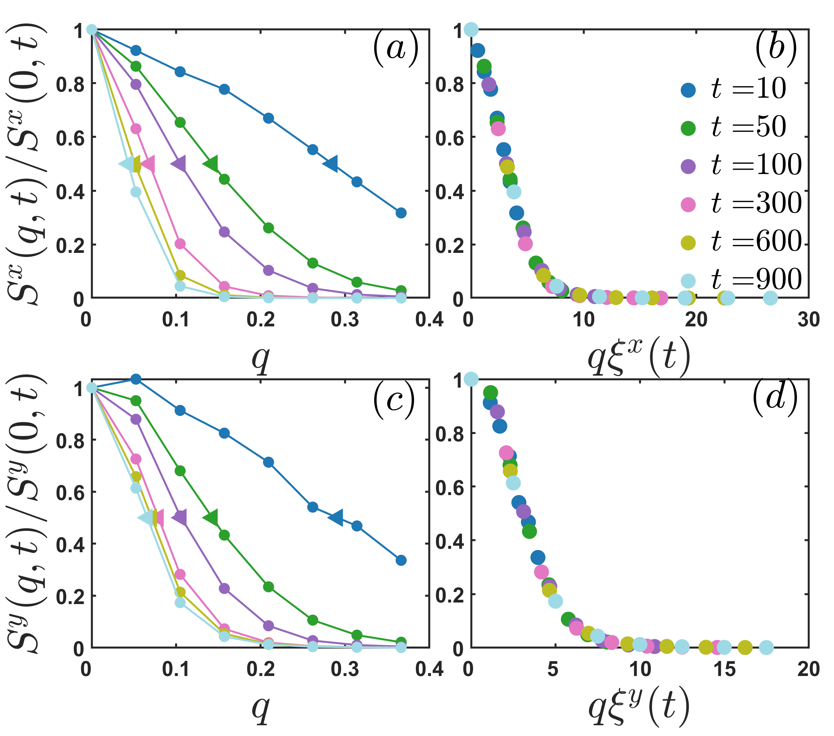
Fig. 5a&c illustrate the time evolution of the structure factors along the direction. We estimate the location of the half width at half maximum, , by a simple linear interpolation (triangular markers). Because the Bragg peaks become quite narrow at late time, only two momentum points are useable for the presented system size (data for and ). This results in a larger degrees of uncertainty in determining , which, in turn, translates to larger uncertainty in estimating the correlation length .
We may approximately collapse the structure factors at different times by plotting them as functions of (Fig. 5b&d). The data collapse of is consistent with the scaling invariance of the phase ordering process. However, we are unable to make any reliable statements about the Prod’s law due to limited system size.
Acknowledgements.
This work is supported by the National Key R&D Program of China (Grant No. 2022YFA1403800), National Natural Science Foundation of China (Grant No. 12250008, 11974396, and 12188101), and by the Chinese Academy of Sciences through the Strategic Priority Research Program (Grant No. XDB33020300).References
- Giannetti et al. [2016] C. Giannetti, M. Capone, D. Fausti, M. Fabrizio, F. Parmigiani, and D. Mihailovic, Advances in Physics 65, 58 (2016).
- Basov et al. [2017] D. N. Basov, R. D. Averitt, and D. Hsieh, Nature Materials 16, 1077 (2017).
- de la Torre et al. [2021] A. de la Torre, D. M. Kennes, M. Claassen, S. Gerber, J. W. McIver, and M. A. Sentef, Rev. Mod. Phys. 93, 041002 (2021).
- Shender and Holdsworth [1996] E. F. Shender and P. C. W. Holdsworth, Order by disorder and topology in frustrated magnetic systems, in Fluctuations and Order: The New Synthesis, edited by M. Millonas (Springer US, New York, NY, 1996) pp. 259–279.
- Chalker [2011] J. T. Chalker, Geometrically frustrated antiferromagnets: Statistical mechanics and dynamics, in Introduction to Frustrated Magnetism: Materials, Experiments, Theory, edited by C. Lacroix, P. Mendels, and F. Mila (Springer Berlin Heidelberg, Berlin, Heidelberg, 2011) pp. 3–22.
- Villain et al. [1980] J. Villain, R. Bidaux, J.-P. Carton, and R. Conte, J. Phys. France 41, 1263 (1980).
- Shender [1982] E. F. Shender, JETP 56, 178 (1982).
- Henley [1989] C. L. Henley, Phys. Rev. Lett. 62, 2056 (1989).
- Oka and Kitamura [2019] T. Oka and S. Kitamura, Annual Review of Condensed Matter Physics 10, 387 (2019).
- Wan and Moessner [2017] Y. Wan and R. Moessner, Phys. Rev. Lett. 119, 167203 (2017).
- Wan and Moessner [2018] Y. Wan and R. Moessner, Phys. Rev. B 98, 184432 (2018).
- Sun [2024] Z. Sun, Phys. Rev. B 110, 104301 (2024).
- Becca and Mila [2002] F. Becca and F. Mila, Phys. Rev. Lett. 89, 037204 (2002).
- Tchernyshyov et al. [2002a] O. Tchernyshyov, R. Moessner, and S. L. Sondhi, Phys. Rev. Lett. 88, 067203 (2002a).
- Tchernyshyov et al. [2002b] O. Tchernyshyov, R. Moessner, and S. L. Sondhi, Phys. Rev. B 66, 064403 (2002b).
- Weber et al. [2005] C. Weber, F. Becca, and F. Mila, Phys. Rev. B 72, 024449 (2005).
- Yusupov et al. [2010] R. Yusupov, T. Mertelj, V. V. Kabanov, S. Brazovskii, P. Kusar, J.-H. Chu, I. R. Fisher, and D. Mihailovic, Nature Physics 6, 681 (2010).
- Kung et al. [2013] Y. F. Kung, W.-S. Lee, C.-C. Chen, A. F. Kemper, A. P. Sorini, B. Moritz, and T. P. Devereaux, Phys. Rev. B 88, 125114 (2013).
- Ross Tagaras et al. [2019] M. Ross Tagaras, J. Weng, and R. E. Allen, The European Physical Journal Special Topics 227, 2297 (2019).
- Sun and Millis [2020] Z. Sun and A. J. Millis, Phys. Rev. X 10, 021028 (2020).
- Dolgirev et al. [2020a] P. E. Dolgirev, A. V. Rozhkov, A. Zong, A. Kogar, N. Gedik, and B. V. Fine, Phys. Rev. B 101, 054203 (2020a).
- Dolgirev et al. [2020b] P. E. Dolgirev, M. H. Michael, A. Zong, N. Gedik, and E. Demler, Phys. Rev. B 101, 174306 (2020b).
- Wang et al. [2006] J. Wang, C. Sun, Y. Hashimoto, J. Kono, G. A. Khodaparast, Ł. Cywiński, L. J. Sham, G. D. Sanders, C. J. Stanton, and H. Munekata, Journal of Physics: Condensed Matter 18, R501 (2006).
- Kirilyuk et al. [2010] A. Kirilyuk, A. V. Kimel, and T. Rasing, Rev. Mod. Phys. 82, 2731 (2010).
- Koopmans et al. [2010] B. Koopmans, G. Malinowski, F. Dalla Longa, D. Steiauf, M. Fähnle, T. Roth, M. Cinchetti, and M. Aeschlimann, Nature Materials 9, 259 (2010).
- Bray [1994] A. J. Bray, Advances in Physics 43, 357 (1994).
- Puri [2009] S. Puri, Kinetics of phase transitions, in Kinetics of Phase Transitions, edited by S. Puri and V. Wadhawan (CRC Press, Boca Raton, FL, 2009) pp. 1–62.
- Cugliandolo [2015] L. F. Cugliandolo, Comptes Rendus Physique 16, 257 (2015).
- Schmidt et al. [2002] R. Schmidt, J. Schulenburg, J. Richter, and D. D. Betts, Phys. Rev. B 66, 224406 (2002).
- [30] See supplemental material for details of construction of Landau energy and additional numerical data.
- Hohenberg and Halperin [1977] P. C. Hohenberg and B. I. Halperin, Rev. Mod. Phys. 49, 435 (1977).
- Aharony [1978] A. Aharony, Phys. Rev. B 18, 3328 (1978).
- Minchau and Pelcovits [1985] B. J. Minchau and R. A. Pelcovits, Phys. Rev. B 32, 3081 (1985).
- Feldman [1998] D. E. Feldman, Journal of Physics A: Mathematical and General 31, L177 (1998).
- Horner and Varma [1968] H. Horner and C. M. Varma, Phys. Rev. Lett. 20, 845 (1968).
- Kimura et al. [2006] T. Kimura, J. C. Lashley, and A. P. Ramirez, Phys. Rev. B 73, 220401 (2006).
- Ye et al. [2006] F. Ye, Y. Ren, Q. Huang, J. A. Fernandez-Baca, P. Dai, J. W. Lynn, and T. Kimura, Phys. Rev. B 73, 220404 (2006).
- Plumer [2007] M. L. Plumer, Phys. Rev. B 76, 144411 (2007).
- Wang and Vishwanath [2008] F. Wang and A. Vishwanath, Phys. Rev. Lett. 100, 077201 (2008).
- Quirion et al. [2009] G. Quirion, M. J. Tagore, M. L. Plumer, and O. A. Petrenko, Journal of Physics: Conference Series 145, 012070 (2009).
- Damay et al. [2009] F. Damay, M. Poienar, C. Martin, A. Maignan, J. Rodriguez-Carvajal, G. André, and J. P. Doumerc, Phys. Rev. B 80, 094410 (2009).
- Vecchini et al. [2010] C. Vecchini, M. Poienar, F. Damay, O. Adamopoulos, A. Daoud-Aladine, A. Lappas, J. M. Perez-Mato, L. C. Chapon, and C. Martin, Phys. Rev. B 82, 094404 (2010).
- Giot et al. [2007] M. Giot, L. C. Chapon, J. Androulakis, M. A. Green, P. G. Radaelli, and A. Lappas, Phys. Rev. Lett. 99, 247211 (2007).
- Zorko et al. [2008] A. Zorko, S. El Shawish, D. Arčon, Z. Jagličić, A. Lappas, H. van Tol, and L. C. Brunel, Phys. Rev. B 77, 024412 (2008).
- Zorko et al. [2014] A. Zorko, O. Adamopoulos, M. Komelj, D. Arčon, and A. Lappas, Nature Communications 5, 3222 (2014).
- Han et al. [2008] Y. Han, Y. Shokef, A. M. Alsayed, P. Yunker, T. C. Lubensky, and A. G. Yodh, Nature 456, 898 (2008).
- Fradkin et al. [2015] E. Fradkin, S. A. Kivelson, and J. M. Tranquada, Rev. Mod. Phys. 87, 457 (2015).
- Fernandes et al. [2019] R. M. Fernandes, P. P. Orth, and J. Schmalian, Annual Review of Condensed Matter Physics 10, 133 (2019).