Image Copy Detection for Diffusion Models

Abstract

Images produced by diffusion models are increasingly popular in digital artwork and visual marketing. However, such generated images might replicate content from existing ones and pose the challenge of content originality. Existing Image Copy Detection (ICD) models, though accurate in detecting hand-crafted replicas, overlook the challenge from diffusion models. This motivates us to introduce ICDiff, the first ICD specialized for diffusion models. To this end, we construct a Diffusion-Replication (D-Rep) dataset and correspondingly propose a novel deep embedding method. D-Rep uses a state-of-the-art diffusion model (Stable Diffusion V1.5) to generate $40,000$ image-replica pairs, which are manually annotated into 6 replication levels ranging from $0$ (no replication) to $5$ (total replication). Our method, PDF-Embedding, transforms the replication level of each image-replica pair into a probability density function (PDF) as the supervision signal. The intuition is that the probability of neighboring replication levels should be continuous and smooth. Experimental results show that PDF-Embedding surpasses protocol-driven methods and non-PDF choices on the D-Rep test set. Moreover, by utilizing PDF-Embedding, we find that the replication ratios of well-known diffusion models against an open-source gallery range from $10\%$ to $20\%$. The project is publicly available at https://icdiff.github.io/.

1 Introduction

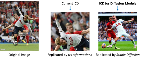
Figure 2: The comparison between current ICD with the ICDiff. The current ICD focuses on detecting edited copies generated by transformations like horizontal flips, random rotations, and random crops. In contrast, the ICDiff aims to detect replication generated by diffusion models, such as Stable Diffusion rombach2021highresolution . (Source of the original image: Lawsuit from Getty Images.)

Diffusion models have gained popularity due to their ability to generate high-quality images. A phenomenon accompanying this trend is that these generated images might replicate content from existing ones. In Fig. 1, we choose six well-known diffusion models midjourney2022 ; new_bing ; ramesh2022hierarchical ; podell2023sdxl ; deep_floyd_IF ; nichol2022glide to illustrate this replication phenomenon. The content replication is acceptable for some (fair) use while interest holders may regard others as copyright infringement lee2024talkin ; somepalli2023diffusion ; wen2024detecting . This paper leaves this dispute alone, and focuses a scientific problem: How to identify the content replication brought by diffusion models?

Image Copy Detection (ICD) provides a general solution to the above demand: it identifies whether an image is copied from a reference gallery after being tampered with. However, the current ICD methods are trained using hand-crafted image transformations (e.g., horizontal flips, random rotations, and random crops) and overlook the challenge from diffusion models. Empirically, we find existing ICD methods can be easily confused by diffusion-generated replicas (as detailed in Table 3). We infer it is because the tamper patterns underlying diffusion-generated replicas (Fig. 2 right) are different from hand-crafted ones (Fig. 2 middle), yielding a considerable pattern gap.

In this paper, we introduce ICDiff, the first ICD specialized for diffusion-generated replicas. Our efforts mainly involve building a new ICD dataset and proposing a novel deep embedding method.

$\bullet$ A Diffusion Replication (D-Rep) dataset. D-Rep consists of $40,000$ image-replica pairs, in which each replica is generated by a diffusion model. Specifically, the images are from LAION-Aesthetic V2 schuhmann2022laion , while their replicas are generated by Stable Diffusion V1.5 rombach2022high . To make the replica generation more efficient, we search out the text prompts (from DiffusionDB wang-etal-2023-diffusiondb )that are similar to the titles of LAION-Aesthetic V2 images, input these text prompts into Stable Diffusion V1.5, and generate many redundant candidate replicas. Given these candidate replicas, we employ human annotators to label the replication level of each generated image against a corresponding LAION-Aesthetic image. The annotation results in $40,000$ image-replica pairs with $6$ replication levels ranging from $0$ (no replication) to $5$ (total replication). We divide D-Rep into a training set with $90\%$ ($36,000$) pairs and a test set with the remaining $10\%$ ($4,000$) pairs.

$\bullet$ A novel method named PDF-Embedding. The ICD methods rely on deep embedding learning at their core. In the deep embedding space, the replica should be close to its original image and far away from other images. Compared with popular deep embedding methods, our PDF-Embedding learns a Probability-Density-Function between two images, instead of a similarity score. More concretely, PDF-Embedding transforms the replication level of each image-replica pair into a PDF as the supervision signal. The intuition is that the probability of neighboring replication levels should be continuous and smooth. For instance, if an image-replica pair is annotated as level-$3$ replication, the probabilities for level-$2$ and level-$4$ replications should also not be significantly low.

PDF-Embedding predicts the probability scores on all the replication levels simultaneously in two steps: 1) extracting $6$ feature vectors in parallel from both the real image and its replica, respectively and 2) calculating $6$ inner products (between two images) to indicate the probability score at $6$ corresponding replication levels. The largest-scored entry indicates the predicted replication level. Experimentally, we prove the effectiveness of our method by comparing it with popular deep embedding models and protocol-driven methods trained on our D-Rep. Moreover, we evaluate the replication of six famous diffusion models and provide a comprehensive analysis.

In conclusion, our key contributions are as follows:

1. We propose a timely and important ICD task, i.e, Image Copy Detection for Diffusion Models (ICDiff), designed specifically to identify the replication caused by diffusion models.

2. We build the first ICDiff dataset and introduce PDF-Embedding as a baseline method. PDF-Embedding transforms replication levels into probability density functions (PDFs) and learns a set of representative vectors for each image.

3. Extensive experimental results demonstrate the efficiency of our proposed method. Moreover, we discover that between $10\%$ to $20\%$ of images generated by six well-known diffusion models replicate contents of a large-scale image gallery.

2 Related Works

2.1 Existing Image Copy Detection Methods

Current ICD methods try to detect replications by learning the invariance of image transformations. For example, ASL wang2023benchmark considers the relationship between image transformations and hard negative samples. AnyPattern wang2024AnyPattern and PE-ICD wang2024peicd build benchmarks and propose solutions that focus on novel patterns in real-world scenarios. SSCD pizzi2022self reveals that self-supervised contrastive training inherently relies on image transformations, and thus adapts InfoNCE oord2018representation by introducing a differential entropy regularization. BoT wang2021bag incorporates approximately ten types of image transformations, combined with various tricks, to train an ICD model. By increasing the intensity of transformations gradually, CNNCL yokoo2021contrastive successfully detects hard positives using a simple contrastive loss and memory bank. EfNet papadakis2021producing ensembles models trained with different image transformations to boost the performance. In this paper, we discover that capturing the invariance of image transformations is ineffective for detecting copies generated by diffusion models. Consequently, we manually label a new dataset and train a specialized ICD model.

2.2 Replication in Diffusion Models

Past research has explored the replication problems associated with diffusion models. The study by somepalli2023diffusion questions if diffusion models generate unique artworks or simply mirror the content from their training data. Research teams from Google, as highlighted in carlini2023extracting , note that diffusion models reveal their training data during content generation. Other studies prevent generating replications from the perspectives of both training diffusion models zhang2023forget ; somepalli2023understanding ; vyas2023provable ; anonymous2023copyright ; zhao2023recipe and copyright holders cui2023ft ; rhodes2023my ; cui2023diffusionshield . Some experts, such as those in somepalli2023understanding , find that the replication of data within training sets might be a significant factor leading to copying behaviors in diffusion models. To address this, webster2023duplication proposes an algorithmic chain to de-duplicate the training sources like LAION-2B schuhmann2022laion . In contrast to these efforts, our ICDiff offers a unique perspective. Specifically, unlike those that directly using existing image descriptors (such as those from CLIP radford2021learning and SSCD pizzi2022self ), we manually-label a dataset and develop a specialized ICD algorithm. By implementing our method, the analytical tools and preventative strategies proposed in existing studies may achieve greater efficacy.

3 Benchmark

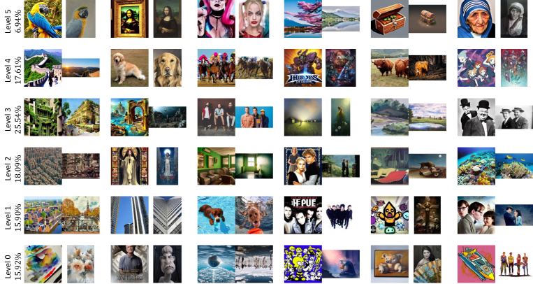
Figure 3: The demonstration of the manual-labeled D-Rep dataset. The percentages on the left show the proportion of images with a particular level.

This section introduces the proposed ICD for diffusion models (ICDiff), including our dataset (D-Rep) and the corresponding evaluation protocols.

3.1 D-Rep Dataset

Current ICD douze2009evaluation ; douze20212021 ; papakipos2022results ; wang2023benchmark ; wang2024peicd ; wang2024AnyPattern primarily focuses on the replica challenges brought by hand-crafted transformations. In contrast, our ICDiff aims to address the replication issues caused by diffusion models midjourney2022 ; new_bing ; ramesh2022hierarchical ; podell2023sdxl ; deep_floyd_IF ; nichol2022glide . To facilitate ICDiff research, we construct D-Rep dataset, which is characterized for diffusion-based replication (See Fig. 3 and the Appendix (Section A) for the examples of diffusion-based replica). The construction process involves generating candidate pairs followed by manual labeling.

Generating candidate pairs. It consists of (1) selecting the top $40,000$ most similar prompts and titles: this selection provides an abundant image-replica pair source. In detail, we use the Sentence Transformer reimers2019sentence to encode the $1.8$ million real-user generated prompts from DiffusionDB wang-etal-2023-diffusiondb and the $12$ million image titles from LAION-Aesthetics V2 6+ schuhmann2022laion , and then utilize the computed cosine similarities to compare; (2) obtaining the candidate pairs: the generated images are produced using the prompts with Stable Diffusion V1.5 rombach2022high , and the real images are fetched based on the titles.

Manual labeling. We generally follow the definition of replication in somepalli2023diffusion and further define six levels of replication (0 to 5). A higher level indicates a greater degree that the generated image replicates the real image. Due to the complex nature of diffusion-generated images, we use multiple levels instead of the binary levels used in somepalli2023diffusion , which employed manual-synthetic datasets as shown in their Fig. 2. We then train ten professional labelers to assign these levels to the $40,000$ candidate pairs: Initially, we assign $4,000$ image pairs to each labeler. If labelers are confident in their judgment of an image pair, they will directly assign a label. Otherwise, they will place the image pair in an undecided pool. On average, each labeler has about $600$ undecided pairs. Finally, for each undecided pair, we vote to reach a final decision. For example, if the votes for an undecided pair are $2$, $2$, $2$, $3$, $3$, $3$, $3$, $3$, $4$, $4$, the final label assigned is $3$. Given the complexity of this labeling task, it took both the labelers and our team one month to finish the process. To maintain authenticity, we did not pre-determine the proportion of each score. The resulting proportions are on the left side of Fig. 3.

3.2 Evaluation Protocols

To evaluate ICD models on the D-Rep dataset, we divide the dataset into a 90/10 training/test split and design two evaluation protocols: Pearson Correlation Coefficient (PCC) and Relative Deviation (RD).

Pearson Correlation Coefficient (PCC). The PCC is a measure used to quantify the linear relationship between two sequences. When PCC is near $1$ or $-1$, it indicates a strong positive or negative relationship. If PCC is near $0$, there’s little to no correlation between the sequences. Herein, we consider two sequences, the predicted replication level $\boldsymbol{s}^{p}=\left(s_{1}^{p},s_{2}^{p},\ldots,s_{n}^{p}\right)$ and the ground-truth $\boldsymbol{s}^{l}=\left(s_{1}^{l},s_{2}^{l},\ldots,s_{n}^{l}\right)$ ($n$ is the number of test pairs). The PCC for ICDiff is defined as:

$$\text{PCC}=\frac{\sum\limits_{i=1}^{n}\left(s^{p}_{i}-\bar{\bm{s}^{p}}\right)\left(s^{l}_{i}-\bar{\bm{s}^{l}}\right)}{\sqrt{\sum\limits_{i=1}^{n}\left(s^{p}_{i}-\bar{\bm{s}^{p}}\right)^{2}}\times\sqrt{\sum\limits_{i=1}^{n}\left(s^{l}_{i}-\bar{\bm{s}^{l}}\right)^{2}}},$$ (1)

where $\bar{\bm{s}^{p}}$ and $\bar{\bm{s}^{l}}$ are the mean values of $\bm{s}^{p}$ and $\bm{s}^{l}$, respectively.

A limitation of the PCC is its insensitivity to global shifts. If all the predictions differ from their corresponding ground truth with the same shift, the PCC does not reflect such a shift and remains large. To overcome this limitation, we propose a new metric called the Relative Deviation (RD).

Relative Deviation (RD). We use RD to quantify the normalized deviation between the predicted and the labeled levels. By normalizing against the maximum possible deviation, RD provides a measure of how close the predictions are to the labeled levels on a scale of $0$ to $1$. The RD is calculated by

$$\text{RD}=\frac{1}{n}\sum^{n}_{i=1}\left(\frac{\left|s^{p}_{i}-s^{l}_{i}\right|}{\max\left(N-s^{l}_{i},s^{l}_{i}\right)}\right),$$ (2)

where $N$ is the highest replication level in our D-Rep.

The Preference for RD over Absolute One. Here we show the preference for employing RD over the absolute one through two illustrative examples. We denote the relative and absolute deviation of the $i$th test pair as: $S_{i}=\frac{\left|s^{p}_{i}-s^{l}_{i}\right|}{\max\left(N-s^{l}_{i},s^{l}_{i}\right)},$ and $T_{i}=\frac{\left|s^{p}_{i}-s^{l}_{i}\right|}{N}.$

(1) For a sample with $s^{l}_{i}=3$, if $s^{p}_{i}=3$, both $S_{i}$ and $T_{i}$ equal $0$; however, if $s^{p}_{i}=0$ (representing the worst prediction), $S_{i}=1$ and $T_{i}=0.6$. Here, $S_{i}$ adjusts the worst prediction to a value of $1$.

(2) In the first scenario, where $s^{l}_{i}=3$ and $s^{p}_{i}=0,S_{i}=1$ and $T_{i}=0.6$. In the second scenario, where $s^{l}_{i}=5$ and $s^{p}_{i}=2,S_{i}=0.6$ and $T_{i}=0.6$. For both cases, $T_{i}$ remains the same at $0.6$, whereas $S_{i}$ values differ. Nevertheless, the two scenarios are distinct: in the first, the prediction cannot deteriorate further; in the second, it can. The value of $S_{i}$ accurately captures this distinction, whereas $T_{i}$ does not.

4 Method

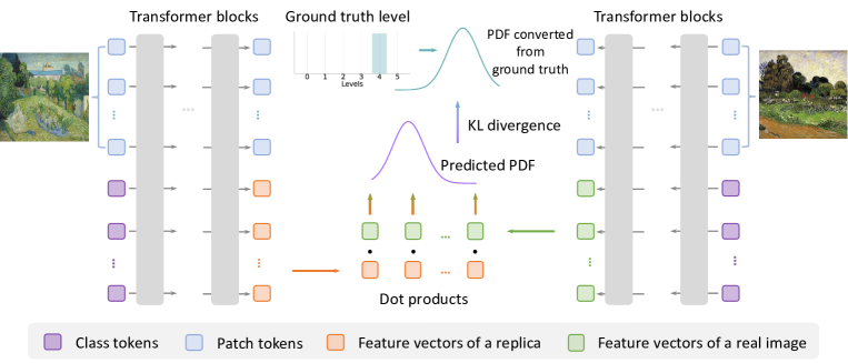
Figure 4: The demonstration of the proposed PDF-Embedding. Initially, PDF-Embedding converts manually-labeled replication levels into probability density functions (PDFs). To learn from these PDFs, we use a set of vectors as the representation of an image.

This section introduces our proposed PDF-Embedding for ICDiff. PDF-Embedding converts each replication level into a probability density function (PDF). To facilitate learning from these PDFs, we expand the original representative vector into a set of vectors. The demonstration of PDF-Embedding is displayed in Fig. 4.

4.1 Converting Level to Probability Density

Given an replication level $s^{l}\in\boldsymbol{s}^{l}$, we first normalize it into $p^{l}=s^{l}/max(\boldsymbol{s}^{l})$. Then we transfer $p^{l}$ into a PDF denoted as $g(x)$ , where $x\in[0,1]$ indicates each possible normalized level. The intuition is that the probability distribution of neighboring replication levels should be continuous and smooth. The function $g(x)$ must satisfy the following conditions: (1) $\int^{1}_{0}g(x)dx=1,$ ensuring that $g(x)$ is a valid PDF; (2) $g(x)\geq 0,$ indicating the non-negativity of the PDF; and (3) $g(x)\leq g(p^{l}),$ which implies that the density is maximized at the normalized level $p^{l}$. We use three different implementations for $g(x)$:

Gaussian:

$$g(x\mid A,\mu,\sigma)=A\cdot\exp\left(-\frac{(x-\mu)^{2}}{2\cdot\sigma^{2}}\right),$$ (3)

linear:

$$g(x\mid A,\mu,\beta)=A-\beta\cdot|x-\mu|,$$ (4)

and exponential:

$$g(x\mid A,\mu,\lambda)=A\cdot\lambda\cdot\exp(-\lambda\cdot|x-\mu|),$$ (5)

where: $A$ is the amplitude, and $\mu$ is the center; $\sigma$ is the standard deviation of Gaussian function, $\beta$ is the slope of linear function, and $\lambda$ is the spread of exponential function.

The performance achieved with various converted PDFs is illustrated in the experimental section. For additional details, please see the Appendix (Section B), which includes (1) the methodology for calculating distribution values, (2) the visualization of the learned distributions corresponding to different image pairs, and (3) an analysis of the deviation rate from peak values.

4.2 Representing an Image as a Set of Vectors

To facilitate learning from the converted PDFs, we utilize a Vision Transformer (ViT) dosovitskiy2020image to represent an image as a set of vectors. Let’s denote the patch tokens from a real image as $\mathbf{X}_{r}^{0}$ and from a generated image as $\mathbf{X}_{g}^{0}$, the ViT model as $f$, and the number of layers in ViT as $L$. The feed-forward process can be expressed as:

$${\left[\mathbf{C}_{r}^{L},\mathbf{X}_{r}^{L}\right]=f\left(\left[\mathbf{C}^{0},\mathbf{X}_{r}^{0}\right]\right),}$$ (6)

$${\left[\mathbf{C}_{g}^{L},\mathbf{X}_{g}^{L}\right]=f\left(\left[\mathbf{C}^{0},\mathbf{X}_{g}^{0}\right]\right),}$$

where $\mathbf{C}^{0}$ is a set of class tokens; $\mathbf{C}_{r}^{L}$ is a set of representative vectors for the real images, consisting of vectors $c_{0,r}^{L},c_{1,r}^{L},\ldots,c_{N,r}^{L}$, and $\mathbf{C}_{g}^{L}$ is a set of representative vectors for the generated images, consisting of vectors $c_{0,g}^{L},c_{1,g}^{L},\ldots,c_{N,g}^{L}$; $N$ is the highest replication level.

Therefore, we can use another PDF $h\left(x\right)$ ($x\in[0,1]$) to describe the predicted replication between two images by

$$h(x)=\mathbf{C}_{r}^{L}\cdot\mathbf{C}_{g}^{L},$$ (7)

which expands to:

$$h(x)=\left[\left\langle\mathbf{c}_{0,r}^{L},\mathbf{c}_{0,g}^{L}\right\rangle,\left\langle\mathbf{c}_{1,r}^{L},\mathbf{c}_{1,g}^{L}\right\rangle,\ldots,\left\langle\mathbf{c}_{N,r}^{L},\mathbf{c}_{N,g}^{L}\right\rangle\right],$$ (8)

where $\langle\cdot,\cdot\rangle$ denotes the cosine similarity.

For training, recalling the PDF $g(x)$ derived from the level, we define the final loss using the Kullback-Leibler (KL) divergence:

$$\mathcal{L}=D_{KL}(g\|h)=\int_{0}^{1}g(x)\log\left(\frac{g(x)}{h(x)}\right)dx,$$ (9)

which serves as a measure of the disparity between two probability distributions. Additionally, in the Appendix (Section C), we demonstrate what the network captures during its learning phase.

During testing, the normalized level between two images is denoted by $\hat{p}^{l}$, satisfying $h(x)\leq h(\hat{p}^{l})$. As illustrated in Eqn. 8, $h(x)$ in practice is discrete within the interval $[0,1]$. Consequently, the resulting level is

$$j=\operatorname{argmax}h(x),$$ (10)

and the normalized level is quantified as $\frac{j}{N}$.

5 Experiments

5.1 Training Details

We implement our PDF-Embedding using PyTorch paszke2019pytorch and distribute its training over 8 A100 GPUs. The ViT-B/16 dosovitskiy2020image serves as the backbone and is pre-trained on the ImageNet dataset deng2009imagenet using DeiT touvron2021training , unless specified otherwise. We resize images to a resolution of $224\times 224$ before training. A batch size of $512$ is used, and the total training epochs is $25$ with a cosine-decreasing learning rate.

5.2 Challenge from the ICDiff Task

Table 1: The performance of publicly available models and our PDF-Embedding on the D-Rep. For qualitative results, please refer to Section E in the Appendix.

Class	Method	PCC ($\%$) $\uparrow$	RD ($\%$) $\downarrow$
Vision-	SLIP mu2022slip	$31.8$	$49.7$
language	BLIP li2022blip	$34.8$	$41.6$
Models	ZeroVL cui2022contrastive	$36.3$	$36.5$
	CLIP radford2021learning	$36.8$	$35.8$
	GPT-4V openai2023gpt4	$47.3$	$38.7$
Self-	SimCLR chen2020simple	$7.2$	$49.4$
supervised	MAE he2022masked	$20.7$	$67.6$
Learning	SimSiam chen2021exploring	$33.5$	$45.4$
Models	MoCov3 he2020momentum	$35.7$	$40.3$
	DINOv2 oquab2023dinov2	$39.0$	$32.9$
Supervised	EfficientNet tan2019efficientnet	$24.0$	$59.3$
Pre-trained	Swin-B liu2021swin	$32.5$	$38.4$
Models	ConvNeXt liu2022convnet	$33.8$	$36.0$
	DeiT-B touvron2021training	$35.3$	$41.7$
	ResNet-50 he2016deep	$37.5$	$34.5$
Current	ASL wang2023benchmark	$5.6$	$78.1$
ICD	CNNCL yokoo2021contrastive	$19.1$	$51.7$
Models	SSCD pizzi2022self	$29.1$	$62.3$
	EfNet papadakis2021producing	$30.5$	$62.8$
	BoT wang2021bag	$35.6$	$53.8$

This section benchmarks popular public models on our D-Rep test dataset. As Table 3 shows, we conduct experiments extensively on vision-language models, self-supervised models, supervised pre-trained models, and current ICD models. We employ these models as feature extractors and calculate the cosine similarity between pairs of image features (except for GPT-4V Turbo openai2023gpt4 , see Section D in the Appendix for the implementation of it). For the computation of PCC and RD, we adjust the granularity by scaling the computed cosine similarities by a factor of $N$. In the Appendix (Section E), we further present the concrete similarities predicted by these models and provide corresponding analysis. We observe that: (1) the large multimodal model GPT-4V Turbo openai2023gpt4 performs best in PCC, while the self-supervised model DINOv2 oquab2023dinov2 excels in RD. This can be attributed to their pre-training on a large, curated, and diverse dataset. Nevertheless, their performance remains somewhat limited, achieving only $47.3\%$ in PCC and $32.9\%$ in RD. This underscores that even the best publicly available models have yet to effectively address the ICDiff task. (2) Current ICD models, like SSCD pizzi2022self , which are referenced in analysis papers somepalli2023diffusion ; somepalli2023understanding discussing the replication issues of diffusion models, indeed show poor performance. For instance, SSCD pizzi2022self registers only $29.1\%$ in PCC and $62.3\%$ in RD. Even the more advanced model, BoT wang2021bag , only manages $35.6\%$ in PCC and $53.8\%$ in RD. These results underscore the need for a specialized ICD method for diffusion models. Adopting our specialized ICD approach will make their subsequent analysis more accurate and convincing. (3) Beyond these models, we also observe that others underperform on the ICDiff task. This further emphasizes the necessity of training a specialized ICDiff model.

5.3 The Effectiveness of PDF-Embedding

This section demonstrates the effectiveness of our proposed PDF-Embedding by (1) contrasting it against protocol-driven methods and non-PDF choices on the D-Rep dataset, (2) comparing between different distributions, and (3) comparing with other models in generalization settings.

Comparison against protocol-driven methods. Since we employ PCC and RD as the evaluation protocols, a natural embedding learning would be directly using these protocols as the optimization objective, i.e., enlarging PCC and reducing RD. Moreover, we add another variant of “reducing RD”, i.e., reducing the absolute deviation $\left|s_{i}^{p}-s_{i}^{l}\right|$ in a regression manner. The comparisons are summarized in Table 2, from which we draw three observations as below: (1) Training on D-Rep with the protocol-driven method achieves good results on their specified protocol but performs bad for the other. While “Enlarging PCC” attains a commendable PCC, its RD of $40.1\%$ indicates large deviation from the ground truth. “Reducing RD” or “Reducing Deviation” shows a relatively good RD ($28.1\%$); however, they exhibit small PCC values that indicate low linear consistency. (2) Our proposed PDF-Embedding surpasses these protocol-driven methods in both PCC and RD. Compared against “Enlarging PCC”, our method improves PCC by $1.6\%$ and decreases RD by $16.1\%$. Besides, our method achieves $+16.0\%$ PCC and $-4.1\%$ RD compared against “Reducing RD” and “Reducing Deviation”. (3) The computational overhead introduced by our method is negligible. First, compared to other options, our method only increases the training time by $5.8\%$. Second, our method introduces minimal additional inference time. Third, while our method requires a longer matching time, its magnitude is close to $10^{-9}$, which is negligible when compared to the inference time’s magnitude of $10^{-3}$. Further discussions on the matching time in real-world scenarios can be found in Section 5.4.

Table 2: Our method demonstrates performance superiority over others.

Method	PCC ($\%$) $\uparrow$	RD ($\%$) $\downarrow$	Train ($s/iter$) $\downarrow$	Infer ($s/img$) $\downarrow$	Match ($s/pair$) $\downarrow$
Enlarging PCC	$54.4$	$40.1$	$0.293$
Reducing RD	$15.1$	$29.9$	$0.294$	$2.02\times 10^{\mathbf{-3}}$	$1.02\times 10^{\mathbf{-9}}$
Regression	$40.3$	$28.1$	$0.292$
One-hot Label	$37.6$	$43.3$	$0.310$	$2.07\times 10^{\mathbf{-3}}$	$6.97\times 10^{\mathbf{-9}}$
Label Smoothing	$35.0$	$36.1$
Ours (Gaussian)	$53.7$	24.0
Ours (Linear)	$54.0$	$24.6$	$0.310$	$2.07\times 10^{\mathbf{-3}}$	$6.97\times 10^{\mathbf{-9}}$
Ours (Exp.)	56.3	$25.6$

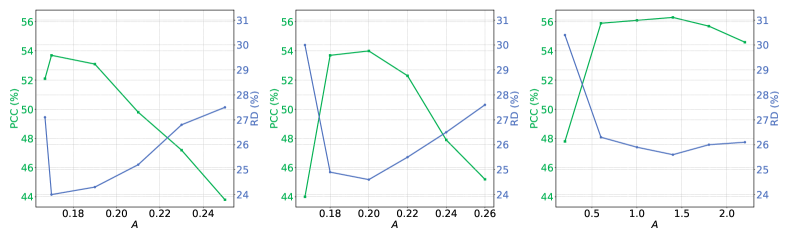
Figure 5: The comparison of different PDFs: Gaussian (left), linear (middle), and exponential (right). “$A$” is the amplitude in each PDF function (Eqn. 3 to Eqn. 5).

Comparison against two non-PDF methods. In Table 2, we also show the experimental results of our method under two standard supervising signals, i.e., “One-hot Label” and “Label Smoothing ($\epsilon=0.5$)”. In comparison, our PDF-Embedding using PDFs gains significant superiority, e.g., using exponential PDF is better than label smoothing by $+21.3\%$ PCC and $-10.5\%$ RD. This superiority validates our intuition that neighboring replication levels should be continuous and smooth.

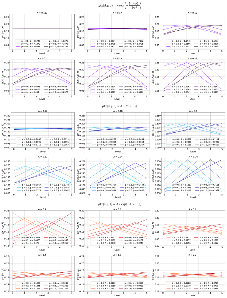
Figure 15: The distributions converted from replication levels. We use Gaussian, linear, and exponential functions as the representative demonstrations.

Comparison between different PDF implementations. We compare between three different PDF implementations for the proposed PDF-Embedding in Fig. 5. We observe that: (1) The exponential (convex) function benefits the PCC metric, whereas the Gaussian (concave) function favors the RD metric. The performance of the linear function, which lacks curvature, falls between that of the convex and concave functions. (2) Our method demonstrates robust performance across various distributions, reducing the challenge of selecting an optimal parameter. For example, when using the exponential function, the performance remains high when $A$ ranges from $0.6$ to $1.8$. (3) A model supervised by a smooth PDF outperforms that supervised by a steeper one (also see the corresponding distributions in Fig. 15 of the Appendix). That consists with our intuition again.

Our model has good generalizability compared to all other methods. Because the collection process of the images from some diffusion models (see Appendix F) differs from the process used to build the test set of our D-Rep dataset, it is difficult to label 6 levels for them and the proposed PCC and RD are not suitable. In the Table 3, we consider a quantitative evaluation protocol that measures the average similarity predicted by a model for given $N$ image pairs, which are manually labeled with the highest level. When normalized to a range of $0$ to $1$, a larger value implies better predictions. This setting is practical because, in the real world, most people’s concerns focus on where replication indeed occurs. We manually confirm $100$ such pairs for each diffusion model. We draw three conclusions: (1) Our PDF-Embedding is more generalizable compared to all zero-shot solutions, such as CLIP, GPT4-V, and DINOv2; (2) Our PDF-Embedding still surpasses all other plausible methods trained on the D-Rep dataset in the generalization setting; (3) Compared against testing on SD1.5 (same domain), for the proposed PDF-Embedding, there is no significant performance drop on the generalization setting.

Table 3: The experiments for “Generalizability to other datasets or diffusion models”. The gray color indicates training and testing on the images generated by the same diffusion model.

Class	Method	SD1.5	Midjo-urney	DAL-L·E 2	DeepFl-oyd IF	New Bing	SDXL	GLIDE
Vision-	SLIP mu2022slip	0.685	0.680	0.668	0.710	0.688	0.718	0.699
language	BLIP li2022blip	0.703	0.674	0.673	0.696	0.696	0.717	0.689
Models	ZeroVL cui2022contrastive	0.578	0.581	0.585	0.681	0.589	0.677	0.707
	CLIP radford2021learning	0.646	0.665	0.694	0.728	0.695	0.735	0.727
	GPT-4V openai2023gpt4	0.661	0.655	0.705	0.731	0.732	0.747	0.744
Self-	SimCLR chen2020simple	0.633	0.640	0.644	0.656	0.649	0.651	0.655
supervised	MAE he2022masked	0.489	0.488	0.487	0.492	0.487	0.489	0.490
Learning	SimSiam chen2021exploring	0.572	0.611	0.619	0.684	0.620	0.645	0.683
Models	MoCov3 he2020momentum	0.585	0.526	0.535	0.579	0.541	0.554	0.599
	DINOv2 oquab2023dinov2	0.766	0.529	0.593	0.723	0.652	0.734	0.751
Supervised	EfficientNet tan2019efficientnet	0.116	0.185	0.215	0.241	0.171	0.210	0.268
Pre-trained	Swin-B liu2021swin	0.334	0.387	0.391	0.514	0.409	0.430	0.561
Models	ConvNeXt liu2022convnet	0.380	0.429	0.432	0.543	0.433	0.488	0.580
	DeiT-B touvron2021training	0.386	0.478	0.496	0.603	0.528	0.525	0.694
	ResNet-50 he2016deep	0.362	0.436	0.465	0.564	0.450	0.522	0.540
Current	ASL wang2023benchmark	0.183	0.231	0.093	0.122	0.048	0.049	0.436
ICD	CNNCL yokoo2021contrastive	0.201	0.311	0.270	0.347	0.279	0.358	0.349
Models	SSCD pizzi2022self	0.116	0.181	0.180	0.303	0.166	0.239	0.266
	EfNet papadakis2021producing	0.133	0.265	0.267	0.438	0.249	0.340	0.349
	BoT wang2021bag	0.216	0.345	0.346	0.477	0.338	0.401	0.489
Models	Enlarging PCC	0.598	0.510	0.523	0.595	0.506	0.554	0.592
Trained	Reducing RD	0.795	0.736	0.736	0.768	0.729	0.768	0.785
on D-Rep	Regression	0.750	0.694	0.705	0.739	0.704	0.721	0.744
	One-hot Label	0.630	0.376	0.400	0.562	0.500	0.548	0.210
	Label Smoothing	0.712	0.568	0.636	0.628	0.680	0.676	0.548
Ours	Gaussian PDF	0.787	0.754	0.784	0.774	0.774	0.780	0.776
	Linear PDF	0.822	0.758	0.798	0.794	0.782	0.794	0.790
	Exponential PDF	0.831	0.814	0.826	0.804	0.802	0.818	0.794

5.4 Simulated Evaluation of Diffusion Models

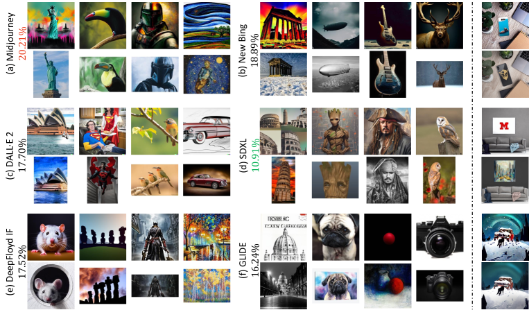
Figure 6: Left: Examples of diffusion-based replication fetched by our PDF-Embedding. The accompanying percentages indicate the replication ratio of each model. Right: Examples filtered by SSCD pizzi2022self in somepalli2023diffusion . Compared to them, our results are more diverse: For example, the “Groot” generated by SDXL includes the whole body, whereas the original one features only the face; and the “Moai statues” created by DeepFloyd IF are positioned differently compared to the original image.

In this section, we simulate a scenario using our trained PDF-Embedding to evaluate popular diffusion models. We select 6 famous diffusion models, of which three are commercial, and another three are open source (See Section F in the Appendix for more details). We use the LAION-Aesthetics V2 6+ dataset schuhmann2022laion as the gallery and investigate whether popular diffusion models replicate it. When assessing the replication ratio of diffusion models, we consider image pairs rated at Level 4 and Level 5 to be replications.

Evaluation results. Visualizations of matched examples and the replication ratios are shown in Fig. 6 (Left). For more visualizations, please refer to the Appendix (Section G). We observe that the replication ratios of these diffusion models roughly range between $10\%$ and $20\%$. The most “aggressive” model is Midjourney midjourney2022 with a rate of $20.21\%$, whereas the “conservative” model is SDXL podell2023sdxl at $10.91\%$. We also include an analysis of failure cases in the Appendix (Section H).

Efficiency analysis. Efficiency is crucial in real-world scenarios. A replication check might slow down the image generation speed of diffusion models. Our PDF-Embedding requires only $2.07\times 10^{-3}$ seconds for inference and an additional $8.36\times 10^{-2}$ seconds for matching when comparing a generated image against a reference dataset of $12$ million images using a standard A100 GPU. This time overhead is negligible compared to the time required for generating (several seconds).

Intuitive comparison with another ICD model. In somepalli2023diffusion , SSCD pizzi2022self is used as a feature extractor to identify replication, as illustrated in Fig. 6 (Right). In comparison, our PDF-Embedding detects a higher number of challenging cases (“hard positives”). Despite visual discrepancies between the generated and original images, replication has indeed occurred.

6 Conclusion

This paper investigates a particular and critical Image Copy Detection (ICD) problem: Image Copy Detection for Diffusion Models (ICDiff). We introduce the first ICDiff dataset and propose a strong baseline called “PDF-Embedding”. A distinctive feature of the D-Rep is its use of replication levels. The dataset annotates each replica into 6 different replication levels. The proposed PDF-Embedding first transforms the annotated level into a probability density function (PDF) to smooth the probability. To learn from the PDFs, our PDF-Embedding adopts a set of representative vectors instead of a traditional representative vector. We hope this work serves as a valuable resource for research on replication in diffusion models and encourages further research efforts in this area.

Disclaimer. The model described herein may yield false positive or negative predictions. Consequently, the contents of this paper should not be construed as legal advice.

Appendix A More examples of the D-Rep Dataset

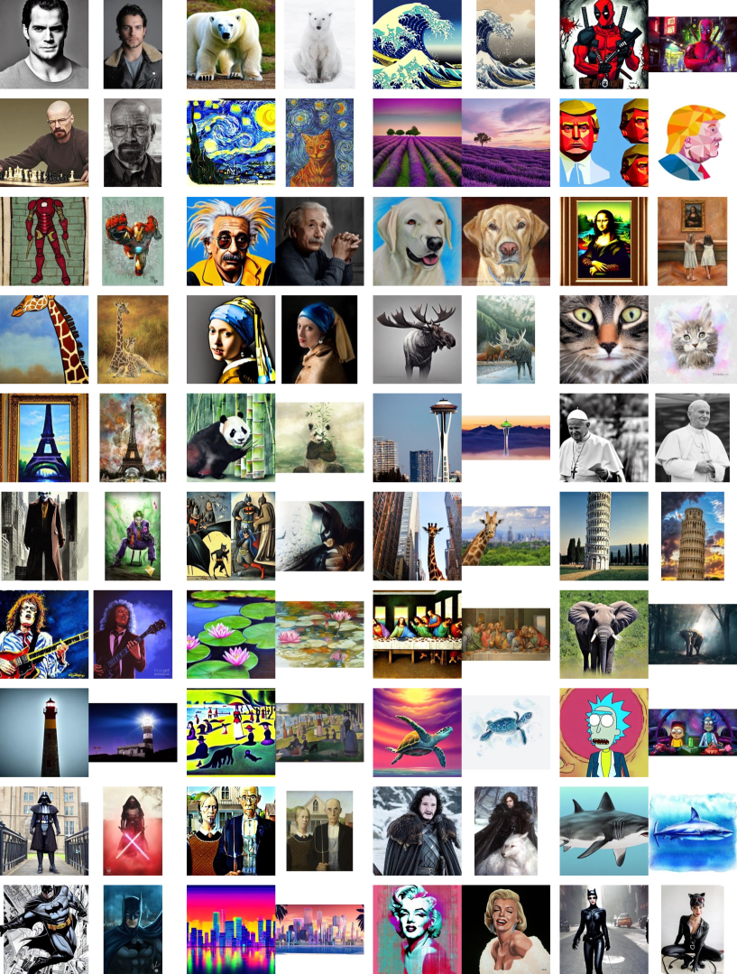
Figure 9: The example image pairs with level $5$.

We show more example image pairs for each level in Fig. 9 to Fig. 14.

Appendix B The Instantiations of PDFs

This section presents examples of PDFs derived from replication levels, focusing on three primary functions: Gaussian, linear, and exponential for our calculations, visualization, and analysis. Within the area close to the normalized level $p^{l}$, denoted as $\delta$, the Gaussian function curves downwards making it concave, the linear function is straight with no curvature, and the exponential function curves upwards making it convex. These characteristics indicate the rate at which they deviate from their peak value: the Gaussian function changes slowly in the $\delta$ area, the linear function changes at a steady rate, and the exponential function changes rapidly in the $\delta$ area. A fast rate of change suggests the network learns from a sharp distribution, while a slow rate implies learning from a smooth distribution.

Gaussian function. Its general formulation is

$$g(x\mid A,\mu,\sigma)=A\cdot\exp\left(-\frac{(x-\mu)^{2}}{2\cdot\sigma^{2}}\right),$$ (11)

where $A>0$ is the amplitude (the height of the peak), $\mu\in\left[0,1\right]$ is the mean or the center, and $\sigma>0$ is the standard deviation. To satisfy the requirements of a PDF in Section 4.1, the following must hold:

$$\begin{gathered}\int^{1}_{0}\left(A\cdot\exp\left(-\frac{(x-\mu)^{2}}{2\cdot\sigma^{2}}\right)\right)dx=1,\\ A\cdot\exp\left(-\frac{(x-\mu)^{2}}{2\cdot\sigma^{2}}\right)\geq 0,\\ A\cdot\exp\left(-\frac{(x-\mu)^{2}}{2\cdot\sigma^{2}}\right)\leq A\cdot\exp\left(-\frac{(p^{l}-\mu)^{2}}{2\cdot\sigma^{2}}\right).\end{gathered}$$ (12)

From Eqn. 12, we have:

$$\mu\ =\ p^{l}.$$ (13)

In practice, with $x\in\left\{0,0.2,0.4,0.6,0.8,1\right\}$ being discrete, the equations become:

$$\begin{gathered}\sum_{x\in\{0,0.2,0.4,0.6,0.8,1\}}\left(A\cdot\exp\left(-\frac{(x-p^{l})^{2}}{2\cdot\sigma^{2}}\right)\right)=1,\\ A\cdot\exp\left(-\frac{(x-p^{l})^{2}}{2\cdot\sigma^{2}}\right)\geq 0.\end{gathered}$$ (14)

Given a specific normalized level $p^{l}$ and varying $A$, $g(x\mid A,\mu,\sigma)$ values are computed for different $x$ using numerical approaches. The resulting distributions are visualized in Fig. 15 (top).

Finally we prove that $g(x\mid A,\mu,\sigma)$ is concave for $x$ in the interval $[\mu-\sigma,\mu+\sigma]$. This means that in the interested region $\delta$ (near the normalized level $p^{l}$), its rate of change is slow and increases as $x$ diverges from $\mu$.

Proof: Given the function:

$$g(x\mid A,\mu,\sigma)=A\exp\left(-\frac{(x-\mu)^{2}}{2\sigma^{2}}\right),$$ (15)

we find the first derivative of $g$ with respect to $x$ :

$$g^{\prime}(x)=\frac{d}{dx}\left[A\exp\left(-\frac{(x-\mu)^{2}}{2\sigma^{2}}\right)\right].$$ (16)

Using the chain rule, we have:

$$g^{\prime}(x)=A\exp\left(-\frac{(x-\mu)^{2}}{2\sigma^{2}}\right)\times\frac{d}{dx}\left[-\frac{(x-\mu)^{2}}{2\sigma^{2}}\right].$$ (17)

This gives:

$$g^{\prime}(x)=-A\exp\left(-\frac{(x-\mu)^{2}}{2\sigma^{2}}\right)\times\frac{(x-\mu)}{\sigma^{2}}.$$ (18)

Next, to find the second derivative, differentiate $g^{\prime}(x)$ with respect to $x$ :

$$g^{\prime\prime}(x)=\frac{d}{dx}\left[-A\exp\left(-\frac{(x-\mu)^{2}}{2\sigma^{2}}\right)\times\frac{(x-\mu)}{\sigma^{2}}\right].$$ (19)

Using product rule and simplifying, the result would be:

$$g^{\prime\prime}(x)=A\exp\left(-\frac{(x-\mu)^{2}}{2\sigma^{2}}\right)\times\left[\frac{(x-\mu)^{2}}{\sigma^{4}}-\frac{1}{\sigma^{2}}\right].$$ (20)

When $g^{\prime\prime}(x)<0$, we have:

$$x\in\left[\mu-\sigma,\mu+\sigma\right].$$ (21)

That proves $g(x\mid A,\mu,\sigma)$ is concave in the $\delta$ area, and thus its rate of change is slow and increases as $x$ diverges from $\mu$.

Linear function. Its general formulation is

$$g(x\mid A,\mu,\beta)=A-\beta\cdot|x-\mu|,$$ (22)

where $A>0$ denotes the maximum value of the function, $\mu\in\left[0,1\right]$ is the point where the function is symmetric, and $\beta>0$ determines the function’s slope. To satisfy the requirements of a PDF in Section 4.1, the following must hold:

$$\begin{gathered}\int^{1}_{0}\left(A-\beta\cdot|x-\mu|\right)dx=1,\\ A-\beta\cdot|x-\mu|\geq 0,\\ A-\beta\cdot|x-\mu|\leq A-\beta\cdot|p^{l}-\mu|.\end{gathered}$$ (23)

From Eqn. 23, we have:

$$\mu\ =\ p^{l}.$$ (24)

In practice, with $x\in\left\{0,0.2,0.4,0.6,0.8,1\right\}$ being discrete, the equations become:

$$\begin{gathered}\sum_{x\in\{0,0.2,0.4,0.6,0.8,1\}}(A-\beta\cdot|x-p^{l}|)=1,\\ A-\beta\cdot|x-p^{l}|\geq 0.\end{gathered}$$ (25)

Given a specific normalized level $p^{l}$ and varying $A$, $g(x\mid A,\mu,\beta)$ values are computed for different $x$. The resulting distributions are visualized in Fig. 15 (middle).

Finally, we prove that $g(x\mid A,\mu,\beta)$ has no curvature, and thus its rate of change is consistent regardless of the value of $x$.

Proof: Given the function:

$$g(x\mid A,\mu,\beta)=A-\beta\cdot|x-\mu|,$$ (26)

we will differentiate this function based on the absolute value, which will result in two cases for the derivatives based on the sign of $(x-\mu)$.

Case 1: $x>\mu$: In this case, $|x-\mu|=x-\mu$. So, $g(x\mid A,\mu,\beta)=A-\beta\cdot(x-\mu)$.

First derivative $g^{\prime}(x)$ :

$$g^{\prime}(x)=\frac{d}{dx}(A-\beta\cdot(x-\mu))=-\beta.$$ (27)

Second derivative $g^{\prime\prime}(x)$ :

$$g^{\prime\prime}(x)=\frac{d}{dx}(-\beta)=0.$$ (28)

Case 2: $x<\mu$: In this case, $|x-\mu|=\mu-x$. So, $g(x\mid A,\mu,\beta)=A-\beta\cdot(\mu-x)$.

First derivative $g^{\prime}(x)$ :

$$g^{\prime}(x)=\frac{d}{dx}(A-\beta\cdot(\mu-x))=\beta.$$ (29)

Second derivative $g^{\prime\prime}(x)$ :

$$g^{\prime\prime}(x)=\frac{d}{dx}(\beta)=0.$$ (30)

When the second derivative is constantly $0$, it means the function has no curvature and its rate of change is constant at every point.

Exponential function. Its general formulation is

$$g(x\mid A,\mu,\lambda)=A\cdot\lambda\cdot\exp(-\lambda\cdot|x-\mu|),$$ (31)

where $A>0$ denotes the intensity of the function, $\mu\in\left[0,1\right]$ is the point where the function is symmetric, and $\lambda>0$ determines the spread or width of the function. To satisfy the requirements of a PDF in Section 4.1, the following must hold:

$$\begin{gathered}\int^{1}_{0}\left(A\cdot\lambda\cdot\exp(-\lambda\cdot|x-\mu|)\right)dx=1,\\ A\cdot\lambda\cdot\exp(-\lambda\cdot|x-\mu|)\geq 0,\\ A\cdot\lambda\cdot\exp(-\lambda\cdot|x-\mu|)\leq A\cdot\lambda\cdot\exp(-\lambda\cdot|p^{l}-\mu|).\end{gathered}$$ (32)

From Eqn. 32, we have:

$$\mu\ =\ p^{l}.$$ (33)

In practice, with $x\in\left\{0,0.2,0.4,0.6,0.8,1\right\}$ being discrete, the equations become:

$$\begin{gathered}\sum_{x\in\{0,0.2,0.4,0.6,0.8,1\}}(A\cdot\lambda\cdot\exp(-\lambda\cdot|x-p^{l}|))=1,\\ A\cdot\lambda\cdot\exp(-\lambda\cdot|x-p^{l}|)\geq 0.\end{gathered}$$ (34)

Given a specific normalized level $p^{l}$ and varying $A$, $g(x\mid A,\mu,\lambda)$ values are computed for different $x$ using numerical approaches. The resulting distributions are visualized in Fig. 15 (bottom).

Finally, we prove that $g(x\mid A,\mu,\lambda)$ is convex: its rate of change is rapid in the $\delta$ area and decreases as $x$ moves diverges from $\mu$.

Proof: Given the function:

$$g(x\mid A,\mu,\lambda)=A\cdot\lambda\cdot\exp(-\lambda\cdot|x-\mu|),$$ (35)

we find the first and second derivatives with respect to $x$. This function involves an absolute value, which will create two cases for the derivatives based on the sign of $(x-\mu)$. Case 1: $x>\mu$: In this case, $|x-\mu|=x-\mu$. So,

$$g(x\mid A,\mu,\lambda)=A\cdot\lambda\cdot\exp(-\lambda\cdot(x-\mu)).$$ (36)

First derivative $g^{\prime}(x)$ :

$$g^{\prime}(x)=A\cdot\lambda\cdot\frac{d}{dx}\exp(-\lambda\cdot(x-\mu)),$$ (37)

$$g^{\prime}(x)=-A\cdot\lambda^{2}\cdot\exp(-\lambda\cdot(x-\mu)).$$

Second derivative $g^{\prime\prime}(x)$ :

$$g^{\prime\prime}(x)=-A\cdot\lambda^{2}\cdot\frac{d}{dx}\exp(-\lambda\cdot(x-\mu)),$$ (38)

$$g^{\prime\prime}(x)=A\cdot\lambda^{3}\cdot\exp(-\lambda\cdot(x-\mu))>0.$$

Case 2: $x<\mu$: In this case, $|x-\mu|=\mu-x$. So,

$$g(x\mid A,\mu,\lambda)=A\cdot\lambda\cdot\exp(-\lambda\cdot(\mu-x)).$$ (39)

First derivative $g^{\prime}(x)$ :

$$g^{\prime}(x)=A\cdot\lambda\cdot\frac{d}{dx}\exp(-\lambda\cdot(\mu-x)),$$ (40)

$$g^{\prime}(x)=A\cdot\lambda^{2}\cdot\exp(-\lambda\cdot(\mu-x)).$$

Second derivative $g^{\prime\prime}(x)$ :

$$g^{\prime\prime}(x)=A\cdot\lambda^{2}\cdot\frac{d}{dx}\exp(-\lambda\cdot(\mu-x)),$$ (41)

$$g^{\prime\prime}(x)=A\cdot\lambda^{3}\cdot\exp(-\lambda\cdot(\mu-x))>0.$$

When the second derivative is bigger than $0$, it means the function is convex: its rate of change is rapid in the $\delta$ area and decreases as $x$ moves diverge from $\mu$.

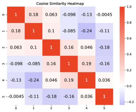
Figure 7: The cosine similarity heatmap of the learned vectors.

Appendix C The Visualization of What the Network Learns

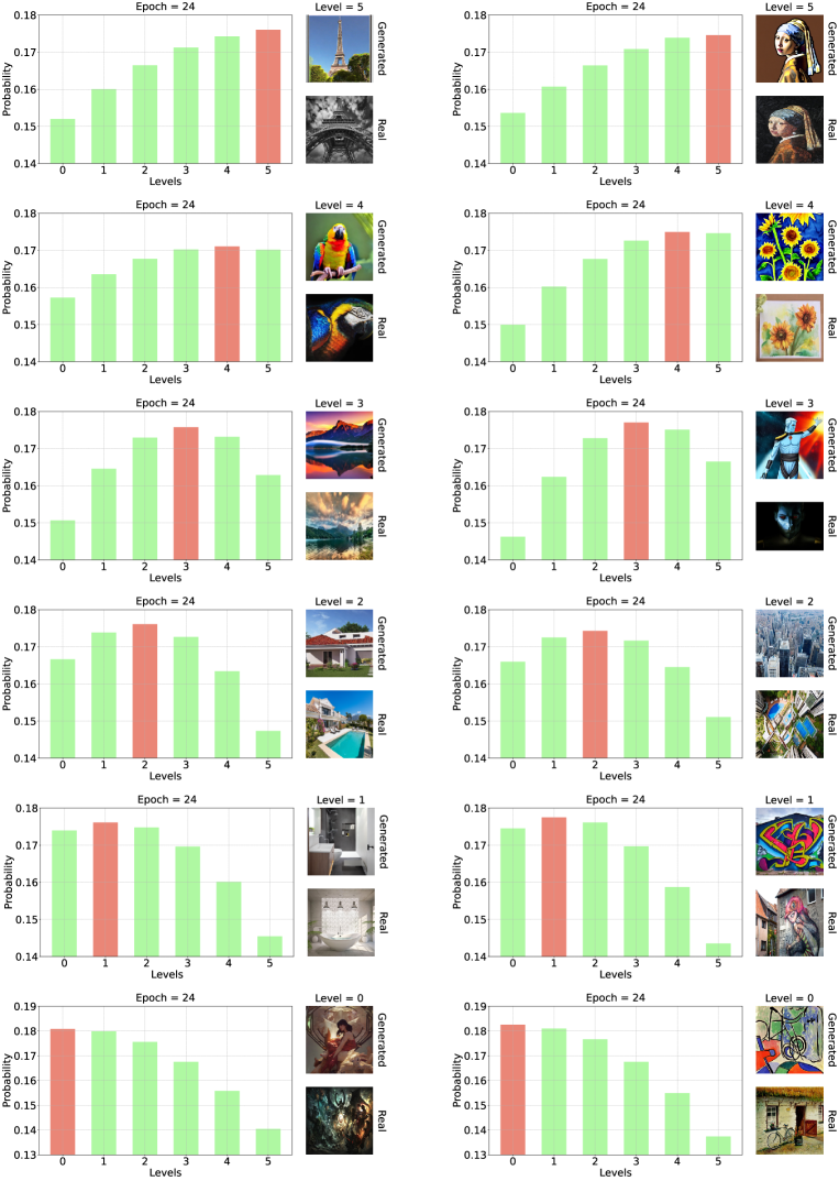
Figure 16: The learned distributions of different image pairs. Please see the attached videos for the distribution changes in the whole training process.

To gain insights into what the network has learned, we offer two visualization methods. First, we present the cosine similarity heatmap of the learned $\mathbf{C}^{0}=\left[\mathbf{c}_{0}^{0},\mathbf{c}_{1}^{0},\ldots,\mathbf{c}_{N}^{0}\right]$ (refer to Fig. 7). Second, we show the distribution changes of image pairs throughout the training process. The final epoch’s distribution can be seen in Fig. 16, while the entire training process is depicted in the attached videos.

From the heatmap, we conclude that: (1) The cosine similarity between different vectors is very low. This demonstrates that the learned vectors are linearly independent. (2) Neighboring vectors exhibit a relatively high cosine similarity. This is consistent with the expectation, as they correspond to similar replication levels.

From the observed changes in the distributions, we note that: (1) While the distribution initially starts as a uniform distribution or peaks at an incorrect level, the network, after training, eventually produces an appropriate and accurate distribution for each image pair. (2) For instance, when supervised by the Gaussian distribution, the network, as expected, produces a final distribution that, though not perfect, closely imitates this.

Appendix D Implement GPT-4V Turbo on our D-Rep Test Dataset

This section details implementing GPT-4V Turbo on our D-Rep test dataset. GPT-4V Turbo, which has been online since November 6, 2023, is the latest and most powerful large multimodal model developed by OpenAI. Because it cannot be regarded as a feature extractor, we directly prompt it with two images and one instruction: Give you one pair of images; please give the similarity of the second one to the first one. Diffusion Models generate the second one, while the first one is the original one. Please only reply with one similarity from $0-1$; no other words are needed. Please understand the images by yourself. Given these prompts, GPT-4V Turbo returns a similarity ranging from $0$ to $1$. Using the official API, we ask the GPT-4V Turbo to determine all similarities between the image pairs in the D-Rep test dataset. Note that the computational cost of employing GPT-4V Turbo in practical applications is prohibitively high. Specifically, to compare an image against an image database containing one million images, the API must be called one million times, incurring a cost of approximately $\$7,800$.

Appendix E The Similarities Predicted by Other Models

In Fig. 17, we show the similarities predicted by six selected models (two vision-language models, two current ICD models, and two others). We conclude that: (1) CLIP radford2021learning tends to assign higher similarities, which deteriorates its performance on image pairs with low levels, leading to many false positive predictions; (2) GPT-4V Turbo openai2023gpt4 and DINOv2 oquab2023dinov2 can produce both high and low predictions, but its performance does not match ours. (3) The prediction ranges of ResNet-50 he2016deep are relatively narrow, indicating its inability to distinguish image pairs with varying levels effectively. (4) Current ICD models, including SSCD pizzi2022self and BoT wang2021bag , consistently produce low predictions. This is because they are trained for invariance to image transformations (resulting in high similarities for pirated content produced by transformations) and cannot handle replication generated by diffusion models.

Appendix F The Details of Six Diffusion Models

This section provides details on the evaluation sources for three commercial and three open-source diffusion models.

Midjourney midjourney2022 was developed by the Midjourney AI company. We utilized a dataset scraped by Succinctly AI under the cc0-1.0 license. This dataset comprises $249,734$ images generated by real users from a public Discord server.

New Bing new_bing , also known as Bing Image Creator, represents Microsoft’s latest text-to-image technique. We utilized the repository under the Unlicense to generate $216,957$ images. These images were produced using randomly selected prompts from DiffusionDB wang-etal-2023-diffusiondb .

DALLE·2 ramesh2022hierarchical is a creation of OpenAI. We downloaded all generated images directly from this website, resulting in a dataset containing $50,904$ images. We have obtained permission from the website’s owners to use the images for research purposes.

We downloaded and deployed three open-source diffusion models, including SDXL podell2023sdxl , DeepFloyd IF deep_floyd_IF , and GLIDE nichol2022glide . These models were set up on a local server equipped with 8 A100 GPUs. Distributing on them, we generated $1,819,792$ images with prompts from DiffusionDB wang-etal-2023-diffusiondb .

Appendix G More Replication Examples

We provide more replication examples by diffusion models in Fig. 18 to Fig. 23.

Appendix H Failure Cases

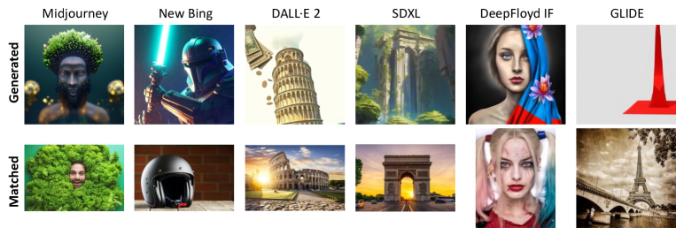
Figure 8: The failure cases of our detection method. We show one example for each diffusion model.

As shown in Fig. 8, we identify two primary failure cases. The first type of failure occurs when the generated images replicate only common elements without constituting replicated content. For instance, elements like grass (Midjourney), helmets (New Bing), and buildings (DALL·E 2) appear frequently but do not indicate actual replication of content. The second type of failure arises when two images share high-level semantic similarity despite having no replicated content. An example can be seen in the image pairs where themes, styles, or concepts are similar, such as the presence of iconic structures (SDXL and GLIDE) or stylized portraits (DeepFloyd IF), even if the specific content is not replicated. Understanding these failure modes is crucial for improving the accuracy and robustness of our detection methods in the future.

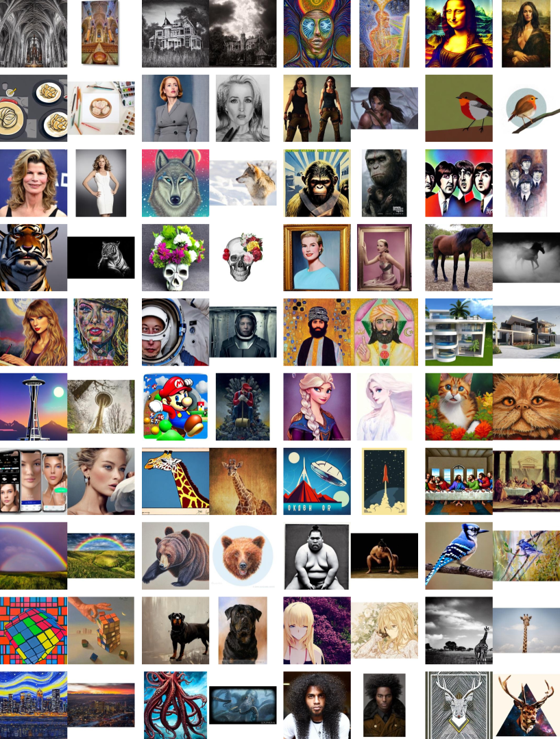
Figure 10: The example image pairs with level $4$.

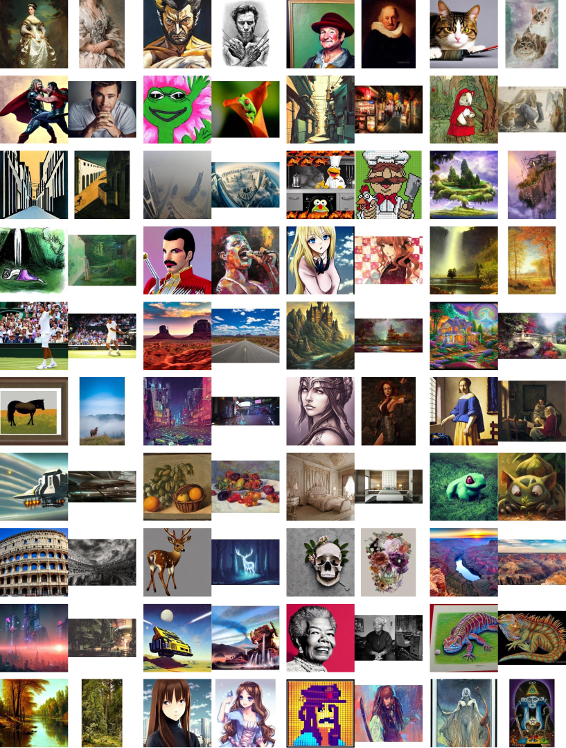
Figure 11: The example image pairs with level $3$.

Figure 12: The example image pairs with level $2$.

Figure 13: The example image pairs with level $1$.

Figure 14: The example image pairs with level $0$.

Method
CLIP
GPT-4V
DINOv2
ResNet-50
SSCD
BoT
Label

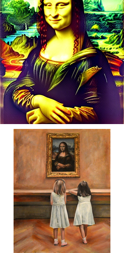
Sim.
0.63
0.40
0.35
0.54
0.04
0.05
1.00

Sim.
0.68
0.60
0.65
0.61
0.16
0.36
1.00

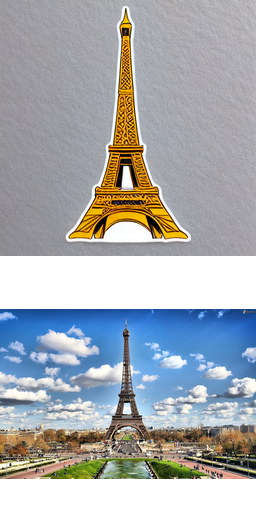
Sim.
0.85
0.30
0.69
0.53
0.08
0.21
1.00

Sim.
0.87
0.90
0.35
0.58
0.10
0.06
1.00

Method
CLIP
GPT-4V
DINOv2
ResNet-50
SSCD
BoT
Label

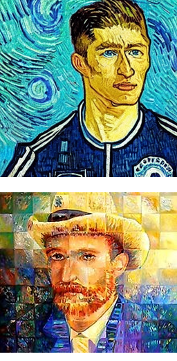
Sim.
0.49
0.70
0.40
0.67
0.11
0.24
0.80

Sim.
0.57
0.20
0.60
0.56
0.13
0.36
0.80

Sim.
0.65
0.00
0.21
0.65
0.00
0.11
0.80

Sim.
0.68
0.30
0.44
0.56
0.12
0.25
0.80

Method
CLIP
GPT-4V
DINOv2
ResNet-50
SSCD
BoT
Label

Sim.
0.70
0.70
0.61
0.60
0.08
0.25
0.60

Sim.
0.71
0.20
0.59
0.60
0.02
0.03
0.60

Sim.
0.82
0.30
0.40
0.57
0.08
0.22
0.60

Sim.
0.93
0.80
0.76
0.62
0.31
0.35
0.60

Method
CLIP
GPT-4V
DINOv2
ResNet-50
SSCD
BoT
Label

Sim.
0.57
0.20
0.28
0.67
0.01
0.21
0.40

Sim.
0.57
0.30
0.58
0.60
0.14
0.21
0.40

Sim.
0.62
0.10
0.23
0.63
0.15
0.25
0.40

Sim.
0.77
0.30
0.55
0.66
0.10
0.16
0.40

Method
CLIP
GPT-4V
DINOv2
ResNet-50
SSCD
BoT
Label

Sim.
0.39
0.00
0.07
0.59
0.06
0.15
0.20

Sim.
0.55
0.00
0.17
0.59
0.02
0.01
0.20

Sim.
0.56
0.00
0.11
0.59
0.05
0.05
0.20

Sim.
0.69
0.00
0.11
0.56
0.12
0.05
0.20

Method
CLIP
GPT-4V
DINOv2
ResNet-50
SSCD
BoT
Label

Sim.
0.38
0.00
0.06
0.61
0.05
0.12
0.00

Sim.
0.56
0.00
0.02
0.62
0.05
0.08
0.00

Sim.
0.57
0.00
0.09
0.53
0.04
0.03
0.00

Sim.
0.78
0.10
0.38
0.63
0.23
0.43
0.00

Figure 17: The similarities (or normalized levels) predicted by existing models.

Figure 18: The replication examples generated by Midjourney midjourney2022 .

Figure 19: The replication examples generated by New Bing new_bing .

Figure 20: The replication examples generated by DALLE·2 ramesh2022hierarchical .

Figure 21: The replication examples generated by SDXL podell2023sdxl .

Figure 22: The replication examples generated by DeepFloyd IF deep_floyd_IF .

Figure 23: The replication examples generated by GLIDE nichol2022glide .

References

- (1) Christoph Schuhmann, Romain Beaumont, Richard Vencu, Cade Gordon, Ross Wightman, Mehdi Cherti, Theo Coombes, Aarush Katta, Clayton Mullis, Mitchell Wortsman, et al. Laion-5b: An open large-scale dataset for training next generation image-text models. Advances in Neural Information Processing Systems, 35:25278–25294, 2022.
- (2) Robin Rombach, Andreas Blattmann, Dominik Lorenz, Patrick Esser, and Björn Ommer. High-resolution image synthesis with latent diffusion models, 2021.
- (3) Midjourney. Midjourney.com, 2022. Accessed: 2023-10-10.
- (4) The new bing, 2023. Accessed: October 10, 2023.
- (5) Aditya Ramesh, Prafulla Dhariwal, Alex Nichol, Casey Chu, and Mark Chen. Hierarchical text-conditional image generation with clip latents. arXiv preprint arXiv:2204.06125, 2022.
- (6) Dustin Podell, Zion English, Kyle Lacey, Andreas Blattmann, Tim Dockhorn, Jonas Müller, Joe Penna, and Robin Rombach. Sdxl: Improving latent diffusion models for high-resolution image synthesis. arXiv preprint arXiv:2307.01952, 2023.
- (7) Deep-floyd. If, 2023. Accessed: October 10, 2023.
- (8) Alexander Quinn Nichol, Prafulla Dhariwal, Aditya Ramesh, Pranav Shyam, Pamela Mishkin, Bob Mcgrew, Ilya Sutskever, and Mark Chen. Glide: Towards photorealistic image generation and editing with text-guided diffusion models. In International Conference on Machine Learning, pages 16784–16804. PMLR, 2022.
- (9) Katherine Lee, A Feder Cooper, and James Grimmelmann. Talkin”bout ai generation: Copyright and the generative-ai supply chain (the short version). In Proceedings of the Symposium on Computer Science and Law, pages 48–63, 2024.
- (10) Gowthami Somepalli, Vasu Singla, Micah Goldblum, Jonas Geiping, and Tom Goldstein. Diffusion art or digital forgery? investigating data replication in diffusion models. In Proceedings of the IEEE/CVF Conference on Computer Vision and Pattern Recognition, pages 6048–6058, 2023.
- (11) Yuxin Wen, Yuchen Liu, Chen Chen, and Lingjuan Lyu. Detecting, explaining, and mitigating memorization in diffusion models. In The Twelfth International Conference on Learning Representations, 2024.
- (12) Robin Rombach, Andreas Blattmann, Dominik Lorenz, Patrick Esser, and Björn Ommer. High-resolution image synthesis with latent diffusion models. In Proceedings of the IEEE/CVF conference on computer vision and pattern recognition, pages 10684–10695, 2022.
- (13) Zijie J. Wang, Evan Montoya, David Munechika, Haoyang Yang, Benjamin Hoover, and Duen Horng Chau. DiffusionDB: A large-scale prompt gallery dataset for text-to-image generative models. In Proceedings of the 61st Annual Meeting of the Association for Computational Linguistics (Volume 1: Long Papers), pages 893–911, Toronto, Canada, July 2023. Association for Computational Linguistics.
- (14) Wenhao Wang, Yifan Sun, and Yi Yang. A benchmark and asymmetrical-similarity learning for practical image copy detection. In Proceedings of the AAAI Conference on Artificial Intelligence, volume 37, pages 2672–2679, 2023.
- (15) Ed Pizzi, Sreya Dutta Roy, Sugosh Nagavara Ravindra, Priya Goyal, and Matthijs Douze. A self-supervised descriptor for image copy detection. In Proceedings of the IEEE/CVF Conference on Computer Vision and Pattern Recognition, pages 14532–14542, 2022.
- (16) Aaron van den Oord, Yazhe Li, and Oriol Vinyals. Representation learning with contrastive predictive coding. arXiv preprint arXiv:1807.03748, 2018.
- (17) Wenhao Wang, Weipu Zhang, Yifan Sun, and Yi Yang. Bag of tricks and a strong baseline for image copy detection. arXiv preprint arXiv:2111.08004, 2021.
- (18) Shuhei Yokoo. Contrastive learning with large memory bank and negative embedding subtraction for accurate copy detection. arXiv preprint arXiv:2112.04323, 2021.
- (19) Sergio Manuel Papadakis and Sanjay Addicam. Producing augmentation-invariant embeddings from real-life imagery. arXiv preprint arXiv:2112.03415, 2021.
- (20) Wenhao Wang, Yifan Sun, Zhentao Tan, and Yi Yang. Anypattern: Towards in-context image copy detection. In arXiv preprint arXiv:2404.13788, 2024.
- (21) Wenhao Wang, Yifan Sun, and Yi Yang. Pattern-expandable image copy detection. In International Journal of Computer Vision, 2024.
- (22) Nicolas Carlini, Jamie Hayes, Milad Nasr, Matthew Jagielski, Vikash Sehwag, Florian Tramer, Borja Balle, Daphne Ippolito, and Eric Wallace. Extracting training data from diffusion models. In 32nd USENIX Security Symposium (USENIX Security 23), pages 5253–5270, 2023.
- (23) Eric Zhang, Kai Wang, Xingqian Xu, Zhangyang Wang, and Humphrey Shi. Forget-me-not: Learning to forget in text-to-image diffusion models. arXiv preprint arXiv:2303.17591, 2023.
- (24) Gowthami Somepalli, Vasu Singla, Micah Goldblum, Jonas Geiping, and Tom Goldstein. Understanding and mitigating copying in diffusion models. Advances in Neural Information Processing Systems, 2023.
- (25) Nikhil Vyas, Sham Kakade, and Boaz Barak. Provable copyright protection for generative models. 2023.
- (26) Anonymous. Copyright plug-in market for the text-to-image copyright protection. In Submitted to The Twelfth International Conference on Learning Representations, 2023. under review.
- (27) Yunqing Zhao, Tianyu Pang, Chao Du, Xiao Yang, Ngai-Man Cheung, and Min Lin. A recipe for watermarking diffusion models. arXiv preprint arXiv:2303.10137, 2023.
- (28) Yingqian Cui, Jie Ren, Yuping Lin, Han Xu, Pengfei He, Yue Xing, Wenqi Fan, Hui Liu, and Jiliang Tang. Ft-shield: A watermark against unauthorized fine-tuning in text-to-image diffusion models. arXiv preprint arXiv:2310.02401, 2023.
- (29) Anthony Rhodes, Ram Bhagat, Umur Aybars Ciftci, and Ilke Demir. My art my choice: Adversarial protection against unruly ai. arXiv preprint arXiv:2309.03198, 2023.
- (30) Yingqian Cui, Jie Ren, Han Xu, Pengfei He, Hui Liu, Lichao Sun, and Jiliang Tang. Diffusionshield: A watermark for copyright protection against generative diffusion models. arXiv preprint arXiv:2306.04642, 2023.
- (31) Ryan Webster, Julien Rabin, Loic Simon, and Frederic Jurie. On the de-duplication of laion-2b. arXiv preprint arXiv:2303.12733, 2023.
- (32) Alec Radford, Jong Wook Kim, Chris Hallacy, Aditya Ramesh, Gabriel Goh, Sandhini Agarwal, Girish Sastry, Amanda Askell, Pamela Mishkin, Jack Clark, et al. Learning transferable visual models from natural language supervision. In International conference on machine learning, pages 8748–8763. PMLR, 2021.
- (33) Matthijs Douze, Hervé Jégou, Harsimrat Sandhawalia, Laurent Amsaleg, and Cordelia Schmid. Evaluation of gist descriptors for web-scale image search. In Proceedings of the ACM international conference on image and video retrieval, pages 1–8, 2009.
- (34) Matthijs Douze, Giorgos Tolias, Ed Pizzi, Zoë Papakipos, Lowik Chanussot, Filip Radenovic, Tomas Jenicek, Maxim Maximov, Laura Leal-Taixé, Ismail Elezi, et al. The 2021 image similarity dataset and challenge. arXiv preprint arXiv:2106.09672, 2021.
- (35) Zoë Papakipos, Giorgos Tolias, Tomas Jenicek, Ed Pizzi, Shuhei Yokoo, Wenhao Wang, Yifan Sun, Weipu Zhang, Yi Yang, Sanjay Addicam, et al. Results and findings of the 2021 image similarity challenge. In NeurIPS 2021 Competitions and Demonstrations Track, pages 1–12. PMLR, 2022.
- (36) Nils Reimers and Iryna Gurevych. Sentence-bert: Sentence embeddings using siamese bert-networks. In Proceedings of the 2019 Conference on Empirical Methods in Natural Language Processing and the 9th International Joint Conference on Natural Language Processing (EMNLP-IJCNLP), pages 3982–3992, 2019.
- (37) Alexey Dosovitskiy, Lucas Beyer, Alexander Kolesnikov, Dirk Weissenborn, Xiaohua Zhai, Thomas Unterthiner, Mostafa Dehghani, Matthias Minderer, Georg Heigold, Sylvain Gelly, et al. An image is worth 16x16 words: Transformers for image recognition at scale. In International Conference on Learning Representations, 2020.
- (38) Adam Paszke, Sam Gross, Francisco Massa, Adam Lerer, James Bradbury, Gregory Chanan, Trevor Killeen, Zeming Lin, Natalia Gimelshein, Luca Antiga, et al. Pytorch: An imperative style, high-performance deep learning library. Advances in neural information processing systems, 32, 2019.
- (39) Jia Deng, Wei Dong, Richard Socher, Li-Jia Li, Kai Li, and Li Fei-Fei. Imagenet: A large-scale hierarchical image database. In 2009 IEEE conference on computer vision and pattern recognition, pages 248–255. Ieee, 2009.
- (40) Hugo Touvron, Matthieu Cord, Matthijs Douze, Francisco Massa, Alexandre Sablayrolles, and Hervé Jégou. Training data-efficient image transformers & distillation through attention. In International conference on machine learning, pages 10347–10357. PMLR, 2021.
- (41) Norman Mu, Alexander Kirillov, David Wagner, and Saining Xie. Slip: Self-supervision meets language-image pre-training. In European Conference on Computer Vision, pages 529–544. Springer, 2022.
- (42) Junnan Li, Dongxu Li, Caiming Xiong, and Steven Hoi. Blip: Bootstrapping language-image pre-training for unified vision-language understanding and generation. In International Conference on Machine Learning, pages 12888–12900. PMLR, 2022.
- (43) Quan Cui, Boyan Zhou, Yu Guo, Weidong Yin, Hao Wu, Osamu Yoshie, and Yubo Chen. Contrastive vision-language pre-training with limited resources. In European Conference on Computer Vision, pages 236–253. Springer, 2022.
- (44) OpenAI. Gpt-4 technical report, 2023.
- (45) Ting Chen, Simon Kornblith, Mohammad Norouzi, and Geoffrey Hinton. A simple framework for contrastive learning of visual representations. In International conference on machine learning, pages 1597–1607. PMLR, 2020.
- (46) Kaiming He, Xinlei Chen, Saining Xie, Yanghao Li, Piotr Dollár, and Ross Girshick. Masked autoencoders are scalable vision learners. In Proceedings of the IEEE/CVF conference on computer vision and pattern recognition, pages 16000–16009, 2022.
- (47) Xinlei Chen and Kaiming He. Exploring simple siamese representation learning. In Proceedings of the IEEE/CVF conference on computer vision and pattern recognition, pages 15750–15758, 2021.
- (48) Kaiming He, Haoqi Fan, Yuxin Wu, Saining Xie, and Ross Girshick. Momentum contrast for unsupervised visual representation learning. In Proceedings of the IEEE/CVF conference on computer vision and pattern recognition, pages 9729–9738, 2020.
- (49) Maxime Oquab, Timothée Darcet, Theo Moutakanni, Huy V. Vo, Marc Szafraniec, Vasil Khalidov, Pierre Fernandez, Daniel Haziza, Francisco Massa, Alaaeldin El-Nouby, Russell Howes, Po-Yao Huang, Hu Xu, Vasu Sharma, Shang-Wen Li, Wojciech Galuba, Mike Rabbat, Mido Assran, Nicolas Ballas, Gabriel Synnaeve, Ishan Misra, Herve Jegou, Julien Mairal, Patrick Labatut, Armand Joulin, and Piotr Bojanowski. Dinov2: Learning robust visual features without supervision, 2023.
- (50) Mingxing Tan and Quoc Le. Efficientnet: Rethinking model scaling for convolutional neural networks. In International conference on machine learning, pages 6105–6114. PMLR, 2019.
- (51) Ze Liu, Yutong Lin, Yue Cao, Han Hu, Yixuan Wei, Zheng Zhang, Stephen Lin, and Baining Guo. Swin transformer: Hierarchical vision transformer using shifted windows. In Proceedings of the IEEE/CVF international conference on computer vision, pages 10012–10022, 2021.
- (52) Zhuang Liu, Hanzi Mao, Chao-Yuan Wu, Christoph Feichtenhofer, Trevor Darrell, and Saining Xie. A convnet for the 2020s. In Proceedings of the IEEE/CVF conference on computer vision and pattern recognition, pages 11976–11986, 2022.
- (53) Kaiming He, Xiangyu Zhang, Shaoqing Ren, and Jian Sun. Deep residual learning for image recognition. In Proceedings of the IEEE conference on computer vision and pattern recognition, pages 770–778, 2016.