Explanation of high redshift luminous galaxies from JWST by early dark energy model

Abstract

Recent observations from the James Webb Space Telescope (JWST) have uncovered massive galaxies at high redshifts, with their abundance significantly surpassing expectations. This finding poses a substantial challenge to both galaxy formation models and our understanding of cosmology. Additionally, discrepancies between the Hubble parameter inferred from high-redshift cosmic microwave background (CMB) observations and those derived from low-redshift distance ladder methods have led to what is known as the “Hubble tension”. Among the most promising solutions to this tension are Early Dark Energy (EDE) models. In this study, we employ an axion-like EDE model in conjunction with a universal Salpeter initial mass function to fit the luminosity function derived from JWST data, as well as other cosmological probes, including the CMB, baryon acoustic oscillations (BAO), and the SH0ES local distance ladder. Our findings indicate that JWST observations favor a high energy fraction of EDE, $f_{\text{EDE}}\sim 0.2\pm 0.03$, and a high Hubble constant value of $H_{0}\sim 74.6\pm 1.2$ km/s/Mpc, even in the absence of SH0ES data. This suggests that EDE not only addresses the $H_{0}$ tension but also provides a compelling explanation for the observed abundance of massive galaxies identified by JWST.

I Introduction

Hubble tension is one of the toughest challenges for the $\Lambda$CDM model nowadays. The measurements of the CMB power spectrum by Planck satellite assuming the $\Lambda$CDM model inferred the Hubble constant ($67.4\pm 0.5$) km/s/Mpc [1]. However, observations on Cepheid-calibrated SNeIa find $H_{0}>70$ km/s/Mpc. For example, the SH0ES team reports $73.04\pm 1.04$ km/s/Mpc [2], which has a $\sim 5\sigma$ tension with the Planck results. Since this tension is unlike systematical uncertainties or due to individual observation, modifications to the $\Lambda$CDM model may be required to restore the tension.

Early Dark Energy (EDE) (see e.g. [3, 4, 5, 6, 7, 8, 9, 10, 11, 12, 13, 14, 15, 16, 17]) is one of the classes of modified cosmological models that promise to resolve Hubble tension. In such models, there is an ingredient that behaves like dark energy at a very early time, and then its energy density starts to decay faster than radiation around matter-radiation equality. While the EDE models are able to raise the Hubble constant inferred from the CMB and are favored by some recent ground-based CMB observations [18, 19, 20, 21, 22, 23], they have encountered a number of challenges, especially conflicts with LSS observations [24, 25, 26].

The recent observations by JWST discover massive galaxies at high redshift with number densities far exceeding those predicted by the $\Lambda$CDM model [27, 28]. However, it has been shown that EDE models can lead to a higher abundance of halos [29, 30, 31, 32]. In this work, we employ the method in Ref.[31] and the luminosity function of galaxies based on JWST observations, which contains a large number of galaxies over a wide redshift range.

A number of possible resolutions to explain the outnumbered abundance of the bright galaxies at $z\geq 10$ have been proposed since its observational confirmation by JWST, e.g., high star formation efficiency ([33]), bursty star formation ([34, 35]), AGN activities ([36]), and a non-universal Initial Mass Function (IMF, [37, 38]), which was considered a promising proposition to resolve the tension with no need of significant changes on our current understanding of cosmology. However, its verification has proved difficult.

This approach is motivated by the fact that the typical application of the classical Salpeter IMF and its descendants ([39, 40]) assumes that the Galactic IMF is identical to that of the extragalactic regions ([37]), which may not stand as firm for the galaxies at high redshift, considering the different environments and preconditions under which the star formation processes took place compared to the local Universe. On the contrary, for a non-universal IMF, the higher abundance of bright galaxies could be attributed to the higher contribution of the massive stars (top-heavy, [38]), allowing the $\Lambda$CDM model to remain valid. However, further studies, e.g., [41, 35] suggest that a non-universal IMF may not be enough to resolve this issue, due to the lack of direct observational evidence, and that the stronger stellar feedback may counteract the top-heavier IMF that leads to a trivial change of the final brightness. Bearing the reservations that a non-universal IMF encounters so far, we assume that the IMF remains universal and study if EDE, a cosmological proposition that appears to have been observationally detected in CMB observation, can better resolve the tension of the galaxy abundance between JWST and previous prediction.

This paper is organized as follows. We summarized our methodology and data employed in section II. The results are shown in section III and we discuss them there. Finally, we conclude in section IV.

II Methodology and Data

The constraints on the Hubble constant derived from the CMB data arise mainly from observations of the acoustic peak separation:

$$\theta_{s}=\frac{r_{s}}{D_{A}}\propto r_{s}H_{0}\,,$$ (1)

where $r_{s}$ is the sound horizon and $D_{A}$ is the angular distance to the last scattering surface. While $\theta_{s}$ is well constrained by current CMB observations, a higher $H_{0}$ means a lower $r_{s}$ unless modifications to the evolution of the late Universe alter the relation between $D_{A}$ and $H_{0}$. However, the latter possibility is tightly constrained by observations of BAO and SNeIa, which means that $r_{s}$ needs to be reduced [42, 43, 44, 45]. In the EDE models, extra energy injections before recombination, which lead to a faster expansion of the Universe at that time, reduce the sound horizon $r_{s}$. After that, the energy density of the EDE decays faster than the radiation to avoid breaking the fitting to the CMB. There are many implementations of the EDE model. For simplicity, we consider the original axion-like EDE model [4]. In this model, the EDE is realized by a canonical scalar field with the following potential:

$$V(\phi)=m^{2}f^{2}(1-\cos\theta)^{n}\text{, where }\theta=\phi/f\in[-\pi,\pi]$$ (2)

The field is frozen initially due to the Hubble friction. As the expansion rate of the Universe decreases, it will roll down and oscillate at the bottom of the potential. In this period, the energy density of the EDE decays with the equation of state $w=(n-1)/(n+1)$. It has been shown $n\sim 3$ is favored by observations [4]. Therefore, we fix $n=3$ in this work.

The luminosity function $\differential n/\differential M_{\text{UV}}$ is the number density of galaxies with respect to their absolute magnitude $M_{\text{UV}}$ at the ultraviolet band. Our modeling of the luminosity function is shown in Ref.[7]. Here we briefly provide the key points. The luminosity function can be decomposed into three components:

$$\derivative{n}{M_{\text{UV}}}=\derivative{n}{M_{h}}\derivative{M_{h}}{M_{*}}\derivative{M_{*}}{M_{\text{UV}}}\,,$$ (3)

where $M_{h}$ is the halo mass and $M_{*}$ is the stellar mass. The first part is the halo mass function. We use the Sheth-Mo-Tormen fitting function [46]:

$$f_{\rm SMT}(\sigma)=A\sqrt{2a/\pi}\nu\exp(-a\nu^{2}/2)(1+(a\nu^{2})^{-p})\,,$$ (4)

where $\sigma$ is the standard deviation of the fluctuation of the density in a sphere containing matter with mass $M_{\text{m}}=M_{h}$ and $\nu=\delta_{\text{crit}}/\sigma$. It contains three parameters {$A,a,p$}. As for $\differential M_{h}/\differential M_{*}$, instead of using a linear stellar-to-halo mass ratio $\epsilon$ (a.k.a. star formation efficiency), we utilize the formula in Ref.[47]:

$$\frac{M_{*}}{M_{h}}=2N\left[\left(\frac{M_{h}}{M_{c}}\right)^{-\beta}+\left(\frac{M_{h}}{M_{c}}\right)^{-\gamma}\right]^{-1}\,,$$ (5)

where $N$ is an overall amplitude factor and $M_{c}$ is the characteristic halo mass. Since very rare AGNs were detected at $z\geq 8$ [48, 49], we extrapolate an AGN-free stellar-to-halo mass ratio to $z=12$ by using $\gamma=0.01$. We consider a scaling relation between the halo mass $M_{\ast}$ and the luminosity of a galaxy at the UV band $M_{UV}$

$$M_{\text{UV}}=[\lg(M_{*})-a_{0}]/a_{1}\,.$$ (6)

For consistency, we use the coefficients $a_{0},a_{1}$ given in Ref.[47], based on the fitting till $z\sim 10$. Finally, we take the dust attenuation rule [50] to account for dust absorption in the UV band and re-emission in the IR band:

$$A_{1600}=4.43+1.99\beta\;,$$ (7)

where $A_{1600}$ is the dust attenuation factor at $1600$ Å  and $\beta=-0.17M_{\text{UV}}-5.40$ [51].

We take the luminosity function data observed by JWST in Refs.[52, 53, 54, 55, 56, 57, 58, 58, 59, 60] and only use data points at $z\leq 12$ due to the high photometric redshift uncertainty at higher redshift. The volume differences caused by differences in the distance-redshift relation of different cosmologies are considered. We use the CMB data from Planck 2018 [1], containing TT,TE,EE spectrum, and lensing spectrum. Meanwhile, we include the BAO data from 6dF [61], SDSS DR7 MGS [62], BOSS DR12 [63], eBOSS DR16 [64], which contains measuments based on observations on ELG, LRG, QSO, Ly-$\alpha$ auto-correlation and its cross-correlation with QSO. SNeIa data from the Pantheon+ analysis [65] is also included. In additionally, we also consider the case with the SH0ES data [2] included, which we use the full covariance matrix with Pantheon+. Recently, the DESI team reported the measurement of BAO from their year of observations [66]. We show the impact of their BAO measurements in Appendix A.

parameter	prior
$n_{s}$	$\mathcal{U}[0.8,1.2]$
$H_{0}$	$\mathcal{U}[60,80]$
$\log(10^{10})A_{s}$	$\mathcal{U}[1.61,3.91]$
$\omega_{b}$	$\mathcal{U}[0.01,0.03]$
$\omega_{\text{cdm}}$	$\mathcal{U}[0.1,0.15]$
$\tau_{\text{reio}}$	$\mathcal{U}[0.01,0.8]$
$\ln z_{c}$	$\mathcal{U}[7.5,9]$
$f_{\text{EDE}}$	$\mathcal{U}[0,0.3]$
$\Theta_{\text{ini}}$	$\mathcal{U}[0,3.1]$
$A$	$\mathcal{N}(0.3295,0.0003)$
$a$	$\mathcal{N}(0.7689,0.0011)$
$p$	$\mathcal{N}(0.2536,0.0026)$
$\log_{10}M_{c}$	$\mathcal{N}(11.5,0.2)$
$N$	$\mathcal{N}(0.0297,0.0065)$
$\beta$	$\mathcal{N}(1.35,0.26)$

Table 1: Parameters and their priors used in our model, see section II for the meaning of these parameters. $\mathcal{U}$ means uniform distribution and $\mathcal{N}(\nu,\sigma)$ means Gaussian distribution.

To perform the joint Bayesian analysis, we utilized cobaya [67] for Markov Chain Monte Carlo (MCMC) sampling. All the chains have reached Gelman-Rubin criterion $R-1<0.03$. Besides the six parameters {$n_{s},H_{0},A_{s},\omega_{\text{b}},\omega_{\text{cdm}},\tau_{\text{reio}}$} for $\Lambda$CDM models, we sample three phenomenological parameters for the axion-like EDE model: the redshift $z_{c}$ when the EDE reached its maximum energy fraction, its energy fraction $f_{\text{EDE}}$ at that time, and the initial position of the axion-like EDE field $\Theta_{\text{ini}}$. The parameters for modeling the luminosity function mentioned above are also sampled. All the parameters for our models and their priors are summarized in Table 1. We use BOBYQA [68, 69] to find the best-fit points.

III Results and Discussion

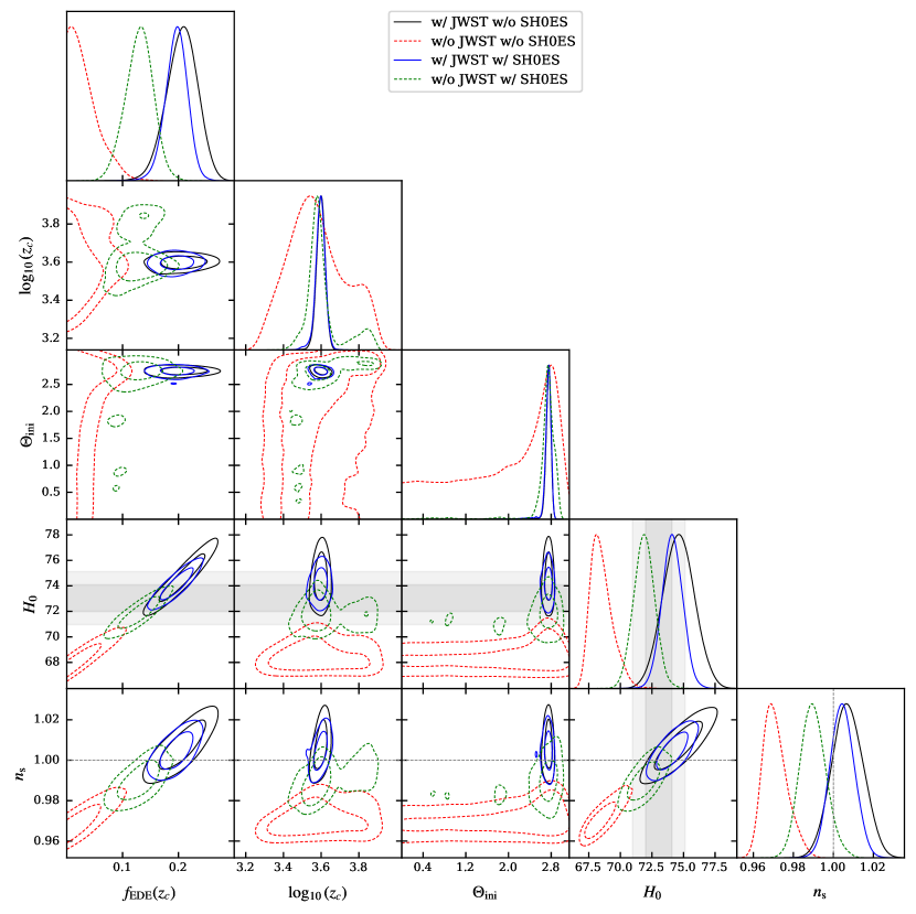
Figure 1: Marginalized posterior distributions for important parameters. The contours show the 68% and 95% confidence levels. We also show the SH0ES [2] constraints on $H_{0}$ in gray bands.

	axionEDE (w/ JWST)	axionEDE (w/o JWST)	$\Lambda$CDM (w/ JWST)	$\Lambda$CDM (w/o JWST)
$\ln(z_{c})$	$8.284(8.238)\pm 0.054$	$8.24(8.120)^{+0.29}_{-0.46}$
$f_{\mathrm{EDE}}(z_{c})$	$0.206(0.2154)^{+0.029}_{-0.026}$	$<0.0412(0.0154)$
$\Theta_{\mathrm{ini}}$	$2.743(2.7734)^{+0.055}_{-0.034}$	$1.94(2.25)^{+1.2}_{-0.44}$
$H_{0}$	$74.6(75.11)\pm 1.2$	$68.51(67.85)^{+0.59}_{-1.0}$	$67.79(67.659)\pm 0.39$	$67.88(68.072)\pm 0.40$
$n_{\mathrm{s}}$	$1.0071(1.0077)\pm 0.0078$	$0.9710(0.9684)^{+0.0046}_{-0.0071}$	$0.9674(0.96700)\pm 0.0036$	$0.9645(0.96616)\pm 0.0037$
$\Omega_{\mathrm{b}}h^{2}$	$0.02295(0.022855)\pm 0.00022$	$0.02252(0.022459)^{+0.00016}_{-0.00020}$	$0.02236(0.022321)\pm 0.00014$	$0.02236(0.022384)\pm 0.00014$
$\Omega_{\mathrm{c}}h^{2}$	$0.1450(0.14618)\pm 0.0044$	$0.1232(0.12145)^{+0.0017}_{-0.0035}$	$0.12028(0.12051)\pm 0.00087$	$0.11997(0.11953)\pm 0.00088$
$\log(10^{10}A_{\mathrm{s}})$	$3.097(3.0870)\pm 0.015$	$3.051(3.0563)\pm 0.015$	$3.062(3.0550)^{+0.014}_{-0.016}$	$3.040(3.0468)\pm 0.014$
$\tau_{\mathrm{reio}}$	$0.0613(0.0552)^{+0.0069}_{-0.0081}$	$0.0552(0.0580)\pm 0.0073$	$0.0624(0.0590)^{+0.0070}_{-0.0081}$	$0.0524(0.0574)\pm 0.0071$
$A$	$0.32949(0.329504)\pm 0.00030$		$0.32949(0.329517)\pm 0.00030$
$a$	$0.7688(0.76886)\pm 0.0011$		$0.7687(0.76870)\pm 0.0011$
$p$	$0.2537(0.25334)\pm 0.0026$		$0.2537(0.25389)\pm 0.0026$
$\log_{10}M_{c}$	$11.52(11.465)^{+0.11}_{-0.13}$		$11.192(11.158)^{+0.085}_{-0.10}$
$N$	$0.0188(0.01729)^{+0.0025}_{-0.0046}$		$0.0249(0.02354)^{+0.0029}_{-0.0042}$
$\beta$	$1.456(1.483)^{+0.077}_{-0.093}$		$1.509(1.517)^{+0.080}_{-0.098}$
$\chi^{2}$	$4437.8$	$4189.1$	$4482.5$	$4189.4$
$\chi^{2}-\chi^{2}_{\text{$\Lambda$CDM}}$	$-44.8$	$-0.3$

Table 2: Marginalized posterior on model parameters where SH0ES data is not included. We show the mean values, 68% confidence levels and put the bestfit values in the parentheses.

	axionEDE (w/ JWST)	axionEDE (w/o JWST)	$\Lambda$CDM (w/ JWST)	$\Lambda$CDM (w/o JWST)
$\ln(z_{c})$	$8.279(8.291)\pm 0.063$	$8.317(8.259)^{+0.047}_{-0.20}$
$f_{\mathrm{EDE}}(z_{c})$	$0.196(0.2107)^{+0.021}_{-0.018}$	$0.130(0.1326)^{+0.026}_{-0.023}$
$\Theta_{\mathrm{ini}}$	$2.734(2.7573)^{+0.066}_{-0.031}$	$2.67(2.742)^{+0.20}_{-0.025}$
$H_{0}$	$74.11(74.71)\pm 0.83$	$71.89(71.98)\pm 0.83$	$68.60(68.714)\pm 0.38$	$68.66(68.558)\pm 0.38$
$n_{\mathrm{s}}$	$1.0045(1.0102)\pm 0.0060$	$0.9899(0.9912)^{+0.0059}_{-0.0068}$	$0.9716(0.97423)\pm 0.0036$	$0.9684(0.96589)\pm 0.0035$
$\Omega_{\mathrm{b}}h^{2}$	$0.02292(0.022967)\pm 0.00022$	$0.02283(0.022797)^{+0.00020}_{-0.00023}$	$0.02253(0.022598)\pm 0.00013$	$0.02253(0.022539)\pm 0.00013$
$\Omega_{\mathrm{c}}h^{2}$	$0.1435(0.14571)\pm 0.0034$	$0.1333(0.13371)^{+0.0032}_{-0.0036}$	$0.11865(0.11852)\pm 0.00083$	$0.11840(0.11872)\pm 0.00084$
$\log(10^{10}A_{\mathrm{s}})$	$3.094(3.0970)\pm 0.015$	$3.069(3.0752)\pm 0.014$	$3.072(3.0875)^{+0.015}_{-0.017}$	$3.047(3.0402)\pm 0.015$
$\tau_{\mathrm{reio}}$	$0.0607(0.0610)^{+0.0070}_{-0.0079}$	$0.0564(0.0594)\pm 0.0070$	$0.0686(0.0766)^{+0.0075}_{-0.0090}$	$0.0572(0.0533)^{+0.0067}_{-0.0075}$
$A$	$0.32949(0.329470)\pm 0.00030$		$0.32949(0.329476)\pm 0.00030$
$a$	$0.7688(0.76873)\pm 0.0011$		$0.7687(0.76865)\pm 0.0011$
$p$	$0.2537(0.25362)\pm 0.0026$		$0.2537(0.25383)\pm 0.0026$
$\log_{10}M_{c}$	$11.50(11.516)^{+0.10}_{-0.13}$		$11.181(11.186)^{+0.085}_{-0.099}$
$N$	$0.0191(0.01695)^{+0.0024}_{-0.0045}$		$0.0254(0.02273)^{+0.0028}_{-0.0043}$
$\beta$	$1.460(1.453)^{+0.078}_{-0.093}$		$1.514(1.515)^{+0.084}_{-0.096}$
$\chi^{2}$	$4487.3$	$4242.7$	$4564.6$	$4271.3$
$\chi^{2}-\chi^{2}_{\text{$\Lambda$CDM}}$	$-77.3$	$-28.6$

Table 3: Marginalized posterior on model parameters where SH0ES data is included. We show the mean values, 68% confidence levels and put the bestfit values in the parentheses.

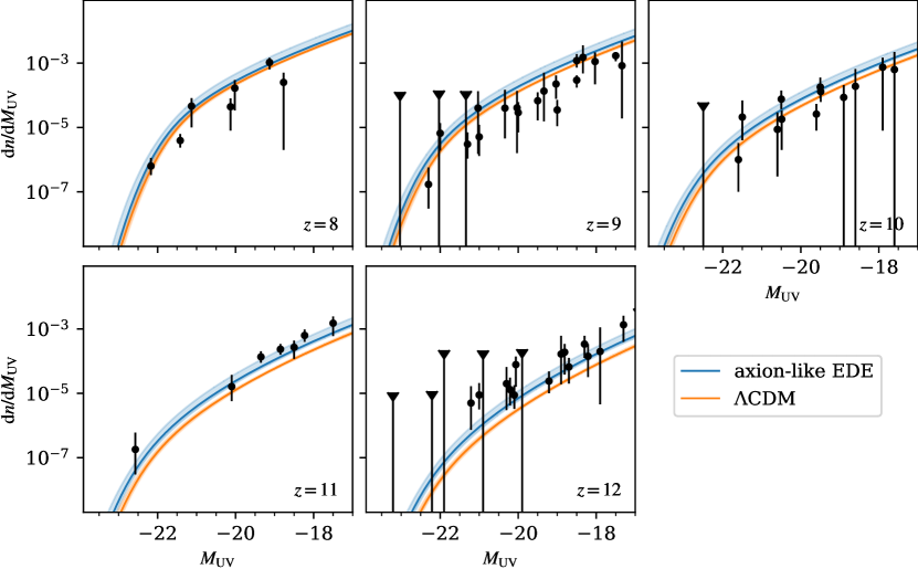
Figure 2: The posterior distribution of the luminosity functions of different models. We also plot the JWST data as error bars. All the values have been corrected to the distance - redshift relationship in the $\Lambda$CDM to allow comparison.

We show the marginalized posterior distribution in Figure 1 and Table 2. We find even when the SH0ES data is not included, a high fraction of EDE $f_{\text{EDE}}=0.206^{+0.029}_{-0.026}$ is favored by the JWST data. The is mainly driven by the JWST data as there is no preference for non-zero $f_{\text{EDE}}$ if we exclude the JWST data (However, see [70, 71] for the discussion of the volume effects). And it leads to $H_{0}=74.6\pm 1.2$ km/s/Mpc, which is slightly higher than the SH0ES result [2] but is consistent within $0.98\sigma$. Meanwhile, we find $n_{s}=1.0071\pm 0.0078$, which is $1\sigma$ consistent with $n_{s}=1$ (see Refs.[23, 72, 73] for the discussion of $n_{s}=1$ in EDE models.). At the best-fit points, we find the EDE model fits the data set better with $\Delta\chi^{2}=-44.8$ compared to the $\Lambda$CDM model, while we only get $\Delta\chi^{2}=-0.3$ if we exclude the JWST data. Even considering the additional parameters of the EDE models, we still get the improvement of Akaike Information Criterium (AIC) $\Delta\text{AIC}=-38.8$. In Figure 2, we show the comparison of the posterior distribution of the luminosity functions with the JWST data, where we can find how the EDE model fits the observations at high redshifts better. However, we find the reduced $\chi^{2}_{\text{JWST}}/{\rm dof}=3.7$ for the EDE model (with dof=62), which means that there may be some unknown uncertainty in the data.

When the SH0ES data is included, as shown in Figure 1 and Table 3, we get a slightly lower mean value of $f_{\text{EDE}}$ but with reduced uncertainty $f_{\text{EDE}}=0.196^{+0.021}_{-0.018}$. The Hubble constant $H_{0}=74.11\pm 0.83$ km/s/Mpc is consistent with the SH0ES result [2] with $0.80\sigma$ and $n_{s}=1.0045\pm 0.0060$ is still within $1\sigma$ of $n_{s}=1$. Since EDE can help resolve the Hubble tension, the improvement of fitting reaches $\Delta\chi^{2}=-77.3$ compared to the $\Lambda$CDM model with the same data set. This conrespoding to $\Delta\text{AIC}=-71.3$.

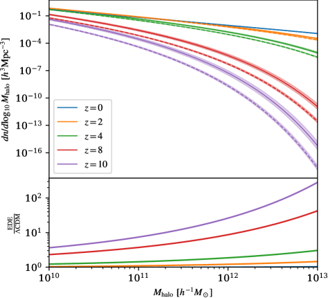
Figure 3: Top: The solid and dashed lines are the halo mass functions of the best-fit points for the EDE and $\Lambda$CDM models for the dataset CMB+BAO+SNe+JWST, respectively. The bands are the 68% confidence interval of the posterior distribution. Bottom: The relative difference in their halo mass function at the best-fit points points.

We show in Figure 3 the effect of the EDE model on the halo mass function, which is positively correlated with the observed luminosity function $\derivative{n}{M_{\text{UV}}}$ as shown in section II. It is clear that the EDE model leads to more massive halos at high redshifts which is exactly what the JWST observations have found. This can be understood by the behavior of the SMT fitting function Equation 4. Since the halo mass function decays exponentially ($\sim\exp(-a\nu^{2}/2)$, which is due to the Gaussianity of the cosmological perturbations) with respect to $\nu=\delta_{\text{crit}}/\sigma$, the relative change of the halo mass function with respect to the matter density fluctuation $\sigma$ will be $\sim\sigma^{-3}$, which means that as the fluctuation $\sigma$ gets smaller, the halo mass function becomes dramatically sensitive to $\sigma$. Meanwhile, the matter perturbations are smaller at high redshifts compared to low redshifts since the perturbations are gradually growing (with growth factor $D_{+}\sim a$) and they are smaller on large scales than on small scales (with $\sigma_{R}\sim k^{-2}T(k_{R})\sim\ln(0.12k_{R}/k_{\text{eq}})$).

As a result, massive halos, which correspond to large scales, at high redshifts will be more sensitive to changes in the perturbation with respect to light halos, which correspond to small scales, or halos at low redshifts. The desired larger matter perturbations compared to $\Lambda$CDM are accomplished in the EDE model by shifts in two parameters. It is well known that the EDE model leads to a larger $\sigma_{8}$, which is enhanced by about 6% for $f_{\text{EDE}}\sim 0.2$. On the other hand, for the halo mass ranges we are interested in, a higher $n_{s}$ in the EDE model also leads to a comparable contribution. Eventually, we will obtain a larger halo mass function in the EDE model, especially at high redshifts and large masses.

IV Conclusion

We tested the axion-like EDE model using the luminosity function measured using JWST. A six-parameter model is considered to infer the luminosity function from the linear matter power spectrum, which incorporates the SMT halo mass function [46], an AGN-free stellar-to-halo mass ratio [47], and a scaling relation between the stellar mass $M_{\ast}$ and absolute magnitude at the UV band $M_{UV}$ [47]. We find the EDE model can fit the data set including JWST with $\Delta\chi^{2}=-44.8$ compared to the $\Lambda$CDM model even if the SH0ES data is excluded. And when the SH0ES data is included, we get an improvement of fitting $\Delta\chi^{2}=-71.3$. Meanwhile, both cases favor high peak fractions of EDE, which lead to $H_{0}$ consistent with the SH0ES result. These results reveal the EDE models are not only promising solutions for the Hubble tension, but also for the exceeding massive galaxies at high redshift observed by JWST.

The more massive galaxies at high redshift in the EDE model relative to the $\Lambda$CDM model come from a larger matter density fluctuation at the corresponding scales due to its higher $\sigma_{8}$ and $n_{s}$. On the other hand, the extreme sensitivity of the halo mass function at small fluctuations in the matter power spectrum leads to the enhancement of the halo mass function concentrating on high redshift and massive halos.

Appendix A Impact of DESI 2024 BAO measuments

In Figure 4, we show the constraints on the EDE parameters and some $\Lambda$CDM parameters of replacing the SDSS BAO measurements with DESI results [66] (including BGS, LRG, ELG, QSO, Ly-$\alpha$ auto-correlation and its cross-correlation with QSO) by using importance reweighting. We find a weaker constraint on $f_{\text{EDE}}$ and a higher $H_{0}$. This can be understood by the lower $\Omega_{\text{m}}$ preferred by the DESI BAO results. As CMB constrain $\omega_{m}=\Omega_{\text{m}}h^{2}$, it will lead to a higher $H_{0}$. Meanwhile, the DESI BAO results prefer a higher $r_{d}h^{2}$ than SDSS , which will also lead to higher $H_{0}$ when combined with the $r_{d}$ derived from the early Universe. In both cases, the constraints on $H_{0}$ from the CMB are weakened, thus enlarging the space allowed for $f_{\text{EDE}}$.

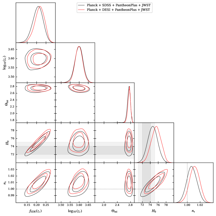
Figure 4: Marginalized posterior distributions for axion-like EDE model with different BAO datasets. The BAO data from 6dF is always included. The contours show the 68% and 95% confidence levels. We also show the SH0ES [2] constraints on $H_{0}$ in gray bands.

References

- Aghanim et al. [2020] N. Aghanim et al. (Planck), Planck 2018 results. VI. Cosmological parameters, Astron. Astrophys. 641, A6 (2020), [Erratum: Astron.Astrophys. 652, C4 (2021)], arXiv:1807.06209 [astro-ph.CO] .
- Riess et al. [2022] A. G. Riess et al., A Comprehensive Measurement of the Local Value of the Hubble Constant with 1 km s-1 Mpc-1 Uncertainty from the Hubble Space Telescope and the SH0ES Team, Astrophys. J. Lett. 934, L7 (2022), arXiv:2112.04510 [astro-ph.CO] .
- Karwal and Kamionkowski [2016] T. Karwal and M. Kamionkowski, Dark energy at early times, the Hubble parameter, and the string axiverse, Phys. Rev. D 94, 103523 (2016), arXiv:1608.01309 [astro-ph.CO] .
- Poulin et al. [2019] V. Poulin, T. L. Smith, T. Karwal, and M. Kamionkowski, Early Dark Energy Can Resolve The Hubble Tension, Phys. Rev. Lett. 122, 221301 (2019), arXiv:1811.04083 [astro-ph.CO] .
- Kaloper [2019] N. Kaloper, Dark energy, and weak gravity conjecture, Int. J. Mod. Phys. D 28, 1944017 (2019), arXiv:1903.11676 [hep-th] .
- Agrawal et al. [2023] P. Agrawal, F.-Y. Cyr-Racine, D. Pinner, and L. Randall, Rock ‘n’ roll solutions to the Hubble tension, Phys. Dark Univ. 42, 101347 (2023), arXiv:1904.01016 [astro-ph.CO] .
- Lin et al. [2019] M.-X. Lin, G. Benevento, W. Hu, and M. Raveri, Acoustic Dark Energy: Potential Conversion of the Hubble Tension, Phys. Rev. D 100, 063542 (2019), arXiv:1905.12618 [astro-ph.CO] .
- Smith et al. [2020] T. L. Smith, V. Poulin, and M. A. Amin, Oscillating scalar fields and the Hubble tension: a resolution with novel signatures, Phys. Rev. D 101, 063523 (2020), arXiv:1908.06995 [astro-ph.CO] .
- Niedermann and Sloth [2021] F. Niedermann and M. S. Sloth, New early dark energy, Phys. Rev. D 103, L041303 (2021), arXiv:1910.10739 [astro-ph.CO] .
- Sakstein and Trodden [2020] J. Sakstein and M. Trodden, Early Dark Energy from Massive Neutrinos as a Natural Resolution of the Hubble Tension, Phys. Rev. Lett. 124, 161301 (2020), arXiv:1911.11760 [astro-ph.CO] .
- Ye and Piao [2020] G. Ye and Y.-S. Piao, Is the Hubble tension a hint of AdS phase around recombination?, Phys. Rev. D 101, 083507 (2020), arXiv:2001.02451 [astro-ph.CO] .
- Gogoi et al. [2021] A. Gogoi, R. K. Sharma, P. Chanda, and S. Das, Early Mass-varying Neutrino Dark Energy: Nugget Formation and Hubble Anomaly, Astrophys. J. 915, 132 (2021), arXiv:2005.11889 [astro-ph.CO] .
- Braglia et al. [2020] M. Braglia, W. T. Emond, F. Finelli, A. E. Gumrukcuoglu, and K. Koyama, Unified framework for early dark energy from -attractors, Phys. Rev. D 102, 083513 (2020), arXiv:2005.14053 [astro-ph.CO] .
- Lin et al. [2020] M.-X. Lin, W. Hu, and M. Raveri, Testing in Acoustic Dark Energy with Planck and ACT Polarization, Phys. Rev. D 102, 123523 (2020), arXiv:2009.08974 [astro-ph.CO] .
- Seto and Toda [2021] O. Seto and Y. Toda, Comparing early dark energy and extra radiation solutions to the Hubble tension with BBN, Phys. Rev. D 103, 123501 (2021), arXiv:2101.03740 [astro-ph.CO] .
- Nojiri et al. [2021] S. Nojiri, S. D. Odintsov, D. Saez-Chillon Gomez, and G. S. Sharov, Modeling and testing the equation of state for (Early) dark energy, Phys. Dark Univ. 32, 100837 (2021), arXiv:2103.05304 [gr-qc] .
- Karwal et al. [2022] T. Karwal, M. Raveri, B. Jain, J. Khoury, and M. Trodden, Chameleon early dark energy and the Hubble tension, Phys. Rev. D 105, 063535 (2022), arXiv:2106.13290 [astro-ph.CO] .
- Chudaykin et al. [2020] A. Chudaykin, D. Gorbunov, and N. Nedelko, Combined analysis of Planck and SPTPol data favors the early dark energy models, JCAP 08, 013, arXiv:2004.13046 [astro-ph.CO] .
- Chudaykin et al. [2021] A. Chudaykin, D. Gorbunov, and N. Nedelko, Exploring an early dark energy solution to the Hubble tension with Planck and SPTPol data, Phys. Rev. D 103, 043529 (2021), arXiv:2011.04682 [astro-ph.CO] .
- Jiang and Piao [2021] J.-Q. Jiang and Y.-S. Piao, Testing AdS early dark energy with Planck, SPTpol, and LSS data, Phys. Rev. D 104, 103524 (2021), arXiv:2107.07128 [astro-ph.CO] .
- La Posta et al. [2022] A. La Posta, T. Louis, X. Garrido, and J. C. Hill, Constraints on prerecombination early dark energy from SPT-3G public data, Phys. Rev. D 105, 083519 (2022), arXiv:2112.10754 [astro-ph.CO] .
- Smith et al. [2022] T. L. Smith, M. Lucca, V. Poulin, G. F. Abellan, L. Balkenhol, K. Benabed, S. Galli, and R. Murgia, Hints of early dark energy in Planck, SPT, and ACT data: New physics or systematics?, Phys. Rev. D 106, 043526 (2022), arXiv:2202.09379 [astro-ph.CO] .
- Jiang and Piao [2022] J.-Q. Jiang and Y.-S. Piao, Toward early dark energy and ns=1 with Planck, ACT, and SPT observations, Phys. Rev. D 105, 103514 (2022), arXiv:2202.13379 [astro-ph.CO] .
- Hill et al. [2020] J. C. Hill, E. McDonough, M. W. Toomey, and S. Alexander, Early dark energy does not restore cosmological concordance, Phys. Rev. D 102, 043507 (2020), arXiv:2003.07355 [astro-ph.CO] .
- Ivanov et al. [2020] M. M. Ivanov, E. McDonough, J. C. Hill, M. Simonović, M. W. Toomey, S. Alexander, and M. Zaldarriaga, Constraining Early Dark Energy with Large-Scale Structure, Phys. Rev. D 102, 103502 (2020), arXiv:2006.11235 [astro-ph.CO] .
- D’Amico et al. [2021] G. D’Amico, L. Senatore, P. Zhang, and H. Zheng, The Hubble Tension in Light of the Full-Shape Analysis of Large-Scale Structure Data, JCAP 05, 072, arXiv:2006.12420 [astro-ph.CO] .
- Labbe et al. [2023] I. Labbe et al., A population of red candidate massive galaxies ~600 Myr after the Big Bang, Nature 616, 266 (2023), arXiv:2207.12446 [astro-ph.GA] .
- Boylan-Kolchin [2023] M. Boylan-Kolchin, Stress testing CDM with high-redshift galaxy candidates, Nature Astron. 7, 731 (2023), arXiv:2208.01611 [astro-ph.CO] .
- Klypin et al. [2021] A. Klypin, V. Poulin, F. Prada, J. Primack, M. Kamionkowski, V. Avila-Reese, A. Rodriguez-Puebla, P. Behroozi, D. Hellinger, and T. L. Smith, Clustering and Halo Abundances in Early Dark Energy Cosmological Models, Mon. Not. Roy. Astron. Soc. 504, 769 (2021), arXiv:2006.14910 [astro-ph.CO] .
- Forconi et al. [2024] M. Forconi, W. Giarè, O. Mena, Ruchika, E. Di Valentino, A. Melchiorri, and R. C. Nunes, A double take on early and interacting dark energy from JWST, JCAP 05, 097, arXiv:2312.11074 [astro-ph.CO] .
- Liu et al. [2024] W. Liu, H. Zhan, Y. Gong, and X. Wang, Can Early Dark Energy be Probed by the High-Redshift Galaxy Abundance?, (2024), arXiv:2402.14339 [astro-ph.CO] .
- Shen et al. [2024] X. Shen, M. Vogelsberger, M. Boylan-Kolchin, S. Tacchella, and R. P. Naidu, Early galaxies and early dark energy: a unified solution to the hubble tension and puzzles of massive bright galaxies revealed by JWST, Mon. Not. Roy. Astron. Soc. 533, 3923 (2024), arXiv:2406.15548 [astro-ph.GA] .
- Dekel et al. [2023] A. Dekel, K. C. Sarkar, Y. Birnboim, N. Mandelker, and Z. Li, Efficient formation of massive galaxies at cosmic dawn by feedback-free starbursts, MNRAS 523, 3201 (2023), arXiv:2303.04827 [astro-ph.GA] .
- Pallottini and Ferrara [2023] A. Pallottini and A. Ferrara, Stochastic star formation in early galaxies: Implications for the James Webb Space Telescope, A&A 677, L4 (2023), arXiv:2307.03219 [astro-ph.GA] .
- Harikane et al. [2024a] Y. Harikane, A. K. Inoue, R. S. Ellis, M. Ouchi, Y. Nakazato, N. Yoshida, Y. Ono, F. Sun, R. A. Sato, S. Fujimoto, N. Kashikawa, D. J. McLeod, P. G. Perez-Gonzalez, M. Sawicki, Y. Sugahara, Y. Xu, S. Yamanaka, A. C. Carnall, F. Cullen, J. S. Dunlop, E. Egami, N. Grogin, Y. Isobe, A. M. Koekemoer, N. Laporte, C.-H. Lee, D. Magee, H. Matsuo, Y. Matsuoka, K. Mawatari, K. Nakajima, M. Nakane, Y. Tamura, H. Umeda, and H. Yanagisawa, JWST, ALMA, and Keck Spectroscopic Constraints on the UV Luminosity Functions at z~7-14: Clumpiness and Compactness of the Brightest Galaxies in the Early Universe, arXiv e-prints , arXiv:2406.18352 (2024a), arXiv:2406.18352 [astro-ph.GA] .
- Harikane et al. [2023] Y. Harikane, Y. Zhang, K. Nakajima, M. Ouchi, Y. Isobe, Y. Ono, S. Hatano, Y. Xu, and H. Umeda, A JWST/NIRSpec First Census of Broad-line AGNs at z = 4-7: Detection of 10 Faint AGNs with M BH 106-108 M ⊙ and Their Host Galaxy Properties, ApJ 959, 39 (2023), arXiv:2303.11946 [astro-ph.GA] .
- Steinhardt et al. [2023] C. L. Steinhardt, V. Kokorev, V. Rusakov, E. Garcia, and A. Sneppen, Templates for Fitting Photometry of Ultra-high-redshift Galaxies, ApJ 951, L40 (2023), arXiv:2208.07879 [astro-ph.GA] .
- Cameron et al. [2024] A. J. Cameron, H. Katz, C. Witten, A. Saxena, N. Laporte, and A. J. Bunker, Nebular dominated galaxies: insights into the stellar initial mass function at high redshift, MNRAS 10.1093/mnras/stae1547 (2024), arXiv:2311.02051 [astro-ph.GA] .
- Salpeter [1955] E. E. Salpeter, The Luminosity Function and Stellar Evolution., ApJ 121, 161 (1955).
- Kroupa and Jerabkova [2019] P. Kroupa and T. Jerabkova, The Salpeter IMF and its descendants, Nature Astronomy 3, 482 (2019), arXiv:1910.01126 [astro-ph.SR] .
- Cueto et al. [2024] E. R. Cueto, A. Hutter, P. Dayal, S. Gottlöber, K. E. Heintz, C. Mason, M. Trebitsch, and G. Yepes, ASTRAEUS. IX. Impact of an evolving stellar initial mass function on early galaxies and reionisation, A&A 686, A138 (2024), arXiv:2312.12109 [astro-ph.GA] .
- Bernal et al. [2016] J. L. Bernal, L. Verde, and A. G. Riess, The trouble with , JCAP 10, 019, arXiv:1607.05617 [astro-ph.CO] .
- Aylor et al. [2019] K. Aylor, M. Joy, L. Knox, M. Millea, S. Raghunathan, and W. L. K. Wu, Sounds Discordant: Classical Distance Ladder & CDM -based Determinations of the Cosmological Sound Horizon, Astrophys. J. 874, 4 (2019), arXiv:1811.00537 [astro-ph.CO] .
- Knox and Millea [2020] L. Knox and M. Millea, Hubble constant hunter’s guide, Phys. Rev. D 101, 043533 (2020), arXiv:1908.03663 [astro-ph.CO] .
- Jiang et al. [2024] J.-Q. Jiang, D. Pedrotti, S. S. da Costa, and S. Vagnozzi, Non-parametric late-time expansion history reconstruction and implications for the Hubble tension in light of DESI, (2024), arXiv:2408.02365 [astro-ph.CO] .
- Sheth et al. [2001] R. K. Sheth, H. J. Mo, and G. Tormen, Ellipsoidal collapse and an improved model for the number and spatial distribution of dark matter haloes, Mon. Not. Roy. Astron. Soc. 323, 1 (2001), arXiv:astro-ph/9907024 .
- Stefanon et al. [2021] M. Stefanon, R. J. Bouwens, I. Labbé, G. D. Illingworth, V. Gonzalez, and P. A. Oesch, Galaxy Stellar Mass Functions from z 10 to z 6 using the Deepest Spitzer/Infrared Array Camera Data: No Significant Evolution in the Stellar-to-halo Mass Ratio of Galaxies in the First Gigayear of Cosmic Time, ApJ 922, 29 (2021), arXiv:2103.16571 [astro-ph.GA] .
- Larson et al. [2023] R. L. Larson et al. (CEERS Team), A CEERS Discovery of an Accreting Supermassive Black Hole 570 Myr after the Big Bang: Identifying a Progenitor of Massive z 6 Quasars, Astrophys. J. Lett. 953, L29 (2023), arXiv:2303.08918 [astro-ph.GA] .
- Scholtz et al. [2023] J. Scholtz, C. Witten, N. Laporte, H. Ubler, M. Perna, R. Maiolino, S. Arribas, W. Baker, J. Bennett, F. D’Eugenio, S. Tacchella, J. Witstok, A. Bunker, S. Carniani, S. Charlot, G. Cresci, E. Curtis-Lake, D. Eisenstein, N. Kumari, B. Robertson, B. Rodriguez Del Pino, C. Simmonds, R. Smit, G. Venturi, C. Williams, and C. Willmer, GN-z11: The environment of an AGN at 10.603, arXiv e-prints , arXiv:2306.09142 (2023), arXiv:2306.09142 [astro-ph.GA] .
- Meurer et al. [1999] G. R. Meurer, T. M. Heckman, and D. Calzetti, Dust absorption and the ultraviolet luminosity density at z~ 3 as calibrated by local starburst galaxies, Astrophys. J. 521, 64 (1999), arXiv:astro-ph/9903054 .
- Cullen et al. [2023] F. Cullen, R. J. McLure, D. J. McLeod, J. S. Dunlop, C. T. Donnan, A. C. Carnall, R. A. A. Bowler, R. Begley, M. L. Hamadouche, and T. M. Stanton, The ultraviolet continuum slopes () of galaxies at z 8-16 from JWST and ground-based near-infrared imaging, MNRAS 520, 14 (2023), arXiv:2208.04914 [astro-ph.GA] .
- Bouwens et al. [2023] R. Bouwens, G. Illingworth, P. Oesch, M. Stefanon, R. Naidu, I. van Leeuwen, and D. Magee, UV luminosity density results at z 8 from the first JWST/NIRCam fields: limitations of early data sets and the need for spectroscopy, Mon. Not. Roy. Astron. Soc. 523, 1009 (2023), arXiv:2212.06683 [astro-ph.CO] .
- Bouwens et al. [2023] R. J. Bouwens, M. Stefanon, G. Brammer, P. A. Oesch, T. Herard-Demanche, G. D. Illingworth, J. Matthee, R. P. Naidu, P. G. van Dokkum, and I. F. van Leeuwen, Evolution of the UV LF from z 15 to z 8 using new JWST NIRCam medium-band observations over the HUDF/XDF, MNRAS 523, 1036 (2023), arXiv:2211.02607 [astro-ph.GA] .
- Castellano et al. [2023] M. Castellano et al., Early Results from GLASS-JWST. XIX. A High Density of Bright Galaxies at z 10 in the A2744 Region, Astrophys. J. Lett. 948, L14 (2023), arXiv:2212.06666 [astro-ph.GA] .
- Donnan et al. [2023] C. T. Donnan, D. J. McLeod, J. S. Dunlop, R. J. McLure, A. C. Carnall, R. Begley, F. Cullen, M. L. Hamadouche, R. A. A. Bowler, D. Magee, H. J. McCracken, B. Milvang-Jensen, A. Moneti, and T. Targett, The evolution of the galaxy UV luminosity function at redshifts z 8 - 15 from deep JWST and ground-based near-infrared imaging, MNRAS 518, 6011 (2023), arXiv:2207.12356 [astro-ph.GA] .
- Finkelstein et al. [2022] S. L. Finkelstein, M. B. Bagley, P. Arrabal Haro, M. Dickinson, H. C. Ferguson, J. S. Kartaltepe, C. Papovich, D. Burgarella, D. D. Kocevski, M. Huertas-Company, K. G. Iyer, A. M. Koekemoer, R. L. Larson, P. G. Pérez-González, C. Rose, S. Tacchella, S. M. Wilkins, K. Chworowsky, A. Medrano, A. M. Morales, R. S. Somerville, L. Y. A. Yung, A. Fontana, M. Giavalisco, A. Grazian, N. A. Grogin, L. J. Kewley, A. Kirkpatrick, P. Kurczynski, J. M. Lotz, L. Pentericci, N. Pirzkal, S. Ravindranath, R. E. Ryan, J. R. Trump, G. Yang, O. Almaini, R. O. Amorín, M. Annunziatella, B. E. Backhaus, G. Barro, P. Behroozi, E. F. Bell, R. Bhatawdekar, L. Bisigello, V. Bromm, V. Buat, F. Buitrago, A. Calabrò, C. M. Casey, M. Castellano, Ó. A. Chávez Ortiz, L. Ciesla, N. J. Cleri, S. H. Cohen, J. W. Cole, K. C. Cooke, M. C. Cooper, A. R. Cooray, L. Costantin, I. G. Cox, D. Croton, E. Daddi, R. Davé, A. de La Vega, A. Dekel, D. Elbaz, V. Estrada-Carpenter, S. M. Faber, V. Fernández, K. D. Finkelstein, J. Freundlich, S. Fujimoto, Á. García-Argumánez, J. P. Gardner, E. Gawiser, C. Gómez-Guijarro, Y. Guo, K. Hamblin, T. S. Hamilton, N. P. Hathi, B. W. Holwerda, M. Hirschmann, T. A. Hutchison, A. E. Jaskot, S. W. Jha, S. Jogee, S. Juneau, I. Jung, S. A. Kassin, A. Le Bail, G. C. K. Leung, R. A. Lucas, B. Magnelli, K. B. Mantha, J. Matharu, E. J. McGrath, D. H. McIntosh, E. Merlin, B. Mobasher, J. A. Newman, D. C. Nicholls, V. Pandya, M. Rafelski, K. Ronayne, P. Santini, L.-M. Seillé, E. A. Shah, L. Shen, R. C. Simons, G. F. Snyder, E. R. Stanway, A. N. Straughn, H. I. Teplitz, B. N. Vanderhoof, J. Vega-Ferrero, W. Wang, B. J. Weiner, C. N. A. Willmer, S. Wuyts, J. A. Zavala, and Ceers Team, A Long Time Ago in a Galaxy Far, Far Away: A Candidate z 12 Galaxy in Early JWST CEERS Imaging, ApJ 940, L55 (2022), arXiv:2207.12474 [astro-ph.GA] .
- Harikane et al. [2023] Y. Harikane, M. Ouchi, M. Oguri, Y. Ono, K. Nakajima, Y. Isobe, H. Umeda, K. Mawatari, and Y. Zhang, A Comprehensive Study of Galaxies at z 9–16 Found in the Early JWST Data: Ultraviolet Luminosity Functions and Cosmic Star Formation History at the Pre-reionization Epoch, Astrophys. J. Suppl. 265, 10.3847/1538-4365/acaaa9 (2023), arXiv:2208.01612 [astro-ph.GA] .
- Harikane et al. [2024b] Y. Harikane, K. Nakajima, M. Ouchi, H. Umeda, Y. Isobe, Y. Ono, Y. Xu, and Y. Zhang, Pure Spectroscopic Constraints on UV Luminosity Functions and Cosmic Star Formation History from 25 Galaxies at z spec = 8.61-13.20 Confirmed with JWST/NIRSpec, ApJ 960, 56 (2024b), arXiv:2304.06658 [astro-ph.GA] .
- Morishita and Stiavelli [2023] T. Morishita and M. Stiavelli, Physical Characterization of Early Galaxies in the Webb’s First Deep Field SMACS J0723.3-7323, ApJ 946, L35 (2023), arXiv:2207.11671 [astro-ph.GA] .
- Pérez-González et al. [2023] P. G. Pérez-González et al., Life beyond 30: Probing the 20 M UV 17 Luminosity Function at 8 z 13 with the NIRCam Parallel Field of the MIRI Deep Survey, Astrophys. J. Lett. 951, L1 (2023), arXiv:2302.02429 [astro-ph.GA] .
- Beutler et al. [2011] F. Beutler, C. Blake, M. Colless, D. H. Jones, L. Staveley-Smith, L. Campbell, Q. Parker, W. Saunders, and F. Watson, The 6dF Galaxy Survey: Baryon Acoustic Oscillations and the Local Hubble Constant, Mon. Not. Roy. Astron. Soc. 416, 3017 (2011), arXiv:1106.3366 [astro-ph.CO] .
- Ross et al. [2015] A. J. Ross, L. Samushia, C. Howlett, W. J. Percival, A. Burden, and M. Manera, The clustering of the SDSS DR7 main Galaxy sample – I. A 4 per cent distance measure at , Mon. Not. Roy. Astron. Soc. 449, 835 (2015), arXiv:1409.3242 [astro-ph.CO] .
- Alam et al. [2017] S. Alam et al. (BOSS), The clustering of galaxies in the completed SDSS-III Baryon Oscillation Spectroscopic Survey: cosmological analysis of the DR12 galaxy sample, Mon. Not. Roy. Astron. Soc. 470, 2617 (2017), arXiv:1607.03155 [astro-ph.CO] .
- Alam et al. [2021] S. Alam et al. (eBOSS), Completed SDSS-IV extended Baryon Oscillation Spectroscopic Survey: Cosmological implications from two decades of spectroscopic surveys at the Apache Point Observatory, Phys. Rev. D 103, 083533 (2021), arXiv:2007.08991 [astro-ph.CO] .
- Brout et al. [2022] D. Brout et al., The Pantheon+ Analysis: Cosmological Constraints, Astrophys. J. 938, 110 (2022), arXiv:2202.04077 [astro-ph.CO] .
- Adame et al. [2024] A. G. Adame et al. (DESI), DESI 2024 VI: Cosmological Constraints from the Measurements of Baryon Acoustic Oscillations, (2024), arXiv:2404.03002 [astro-ph.CO] .
- Torrado and Lewis [2021] J. Torrado and A. Lewis, Cobaya: Code for Bayesian Analysis of hierarchical physical models, JCAP 05, 057, arXiv:2005.05290 [astro-ph.IM] .
- Cartis et al. [2018a] C. Cartis, J. Fiala, B. Marteau, and L. Roberts, Improving the Flexibility and Robustness of Model-Based Derivative-Free Optimization Solvers, arXiv e-prints , arXiv:1804.00154 (2018a), arXiv:1804.00154 [math.OC] .
- Cartis et al. [2018b] C. Cartis, L. Roberts, and O. Sheridan-Methven, Escaping local minima with derivative-free methods: a numerical investigation, arXiv e-prints , arXiv:1812.11343 (2018b), arXiv:1812.11343 [math.OC] .
- Smith et al. [2021] T. L. Smith, V. Poulin, J. L. Bernal, K. K. Boddy, M. Kamionkowski, and R. Murgia, Early dark energy is not excluded by current large-scale structure data, Phys. Rev. D 103, 123542 (2021), arXiv:2009.10740 [astro-ph.CO] .
- Herold et al. [2022] L. Herold, E. G. M. Ferreira, and E. Komatsu, New Constraint on Early Dark Energy from Planck and BOSS Data Using the Profile Likelihood, Astrophys. J. Lett. 929, L16 (2022), arXiv:2112.12140 [astro-ph.CO] .
- Ye et al. [2022] G. Ye, J.-Q. Jiang, and Y.-S. Piao, Toward inflation with ns=1 in light of the Hubble tension and implications for primordial gravitational waves, Phys. Rev. D 106, 103528 (2022), arXiv:2205.02478 [astro-ph.CO] .
- Jiang et al. [2023] J.-Q. Jiang, G. Ye, and Y.-S. Piao, Return of Harrison–Zeldovich spectrum in light of recent cosmological tensions, Mon. Not. Roy. Astron. Soc. 527, L54 (2023), arXiv:2210.06125 [astro-ph.CO] .
- Mukherjee and Sen [2024] P. Mukherjee and A. A. Sen, Model-independent cosmological inference post DESI DR1 BAO measurements, (2024), arXiv:2405.19178 [astro-ph.CO] .