Quantum-inspired Beamforming Optimization for Quantized Phase-only Massive MIMO Arrays

Abstract

This paper introduces an innovative quantum-inspired method for beamforming (BF) optimization in multiple-input multiple-output (MIMO) arrays. The method leverages the simulated bifurcation (SB) algorithm to address the complex combinatorial optimization problem due to the quantized phase configuration. We propose novel encoding techniques for high-bit phase quantization, which are then mapped into Ising spins. This enables efficient construction of the Hamiltonians and subsequent optimization of BF patterns. The results clearly demonstrate that the SB optimizer surpasses traditional schemes such as digital BF, holographic algorithms and genetic algorithms, offering faster convergence and higher solution quality. The impressive capability of the SB optimizer to handle complex BF scenarios, including sidelobe suppression and multiple beams with nulls, is undoubtedly demonstrated through several application cases. These findings strongly suggest that quantum-inspired methods have great potential to advance MIMO techniques in next-generation wireless communication.

Keywords: quantum-inspired method, beamforming, massive MIMO, combinatorial optimization, high-bit phase quantization.

1 Introduction

Multiple-input and multiple-output (MIMO) technology, that is, the use of multiple antennas at the transmitter (TX) and receiver (RX), has attracted much attention in wireless communications. Advances in the MIMO technology result in high data rates, strong signal reliability and large network capacity[1, 2, 3, 4, 5, 6]. Moreover, MIMO technology encompasses a variety of powerful techniques, such as beamforming (BF), that significantly enhance the performance of wireless communication[7, 8, 9]. While MIMO technology has been explored for more than a decade, the seminal work of Marzetta introduced the exciting new concept of “massive MIMO”, where the number of antenna elements at the base station reaches dozens or hundreds[10]. Massive MIMO arrays allow for more concentrated beams directing toward the users, which enables enhanced signal quality, extended coverage and increased capacity[10, 11, 12, 13]. At both the TX and RX, massive MIMO BF is particularly useful to obtain desired array gains, thereby offering both increased signal-to-noise ratio and additional radio link margin that mitigates propagation path loss. This promising technology is expected to play a critical role in 5G mobile systems[14, 15, 16, 17, 18].

However, a large number of elements in massive MIMO arrays also poses major challenges:

• To reduce the hardware cost, most MIMO arrays currently have a quantized phase-only configuration. Quantized phase-only BF can be mapped into an unconstrained combinatorial optimization problem, which is an NP-hard problem. The huge solution space leads to a long optimization time[19, 20, 21].

• There is no known (semi) analytical solution for specific quantized phase-only BF such as single beam, multiple beams, or beams with nulls. The objective function is often designed as an empirical expression related to the figures of merit (such as directivity, sidelobe level, etc.). When the figures of merit are complex, it is easy to fall into a local optimum.

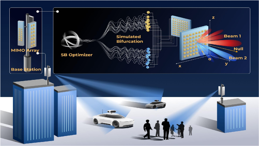
Figure 1: To meet the BF requirements in specific application scenarios, we optimize the phase distribution of the quantized phase-only MIMO array. Firstly, we encode the phases using our innovative encoding technique. Secondly, we map the radiation pattern of the array into the BF Hamiltonian based on the Ising model. Thirdly, we utilise the SB optimizer to simulate the bifurcation phenomenon during the adiabatic evolution of the Hamiltonian, which is a variable-weighted sum of the initial nonlinear Kerr Hamiltonian and final BF Hamiltonian. Finally, we successfully obtain the (near) optimal solution to the BF Hamiltonian, i.e. optimized bit configuration for the phase distribution.

To meet these challenges, a range of BF optimization schemes have been introduced in the literature, including digital BF[22, 23], holographic algorithms[24, 25], genetic algorithms[26, 27], impedance-based synthesis[28], EM inversion[29, 30] and machine learning[31, 32, 33]. Despite these efforts, the above challenges have not been overcome, due to the complicated requirements for BF in real-life scenarios.

Recently, quantum annealing has been proposed to solve EM problems and demonstrated its potential to obtain high-quality solutions in a short optimization time[34, 35, 36, 37]. The Ising model for reconfigurable intelligence surfaces was first introduced and analyzed in 2021[38], in which the BF Hamiltonian represents the total scattered power of the reconfigurable intelligence surface along a specific direction. The 1-bit and 2-bit quantized phase-only BF cases for small-scale reconfigurable intelligence surfaces are shown, confirming the effectiveness of quantum annealing. However, due to limited quantum bit resources and unavoidable bit loss in the embedding process (embedding the Ising Hamiltonian expression into the Chimera graph of the quantum annealer DW2Q), the BF optimization of quantized phase-only massive MIMO arrays utilizing quantum annealing is unachievable at present.

To tackle the scalability issue in BF optimization, a promising solution is to explore the concept of quantum-inspired methods[39, 40, 41, 42]. In this work, we utilize a representative quantum-inspired method called simulated bifurcation (SB) algorithm[43, 44, 45, 46]. Simulating the adiabatic evolution of a classical nonlinear oscillator on a classical computer, SB provides an efficient approach to solving the BF optimization problem in quantized phase-only massive MIMO arrays, as shown in Fig. 1. A specific case involves converting a nonlinear quantum model into a classical model and then solving the equations of motion on a classical computer. To develop such an algorithm, the process can be divided into three steps: Firstly, we create an encoding technique to map the quantized phases into a set of spin variables, and in particular, encoding routes for 1, 2 and 3-bit phase quantization are developed. Secondly, the Hamiltonian of the BF optimization, which is the variable-weighted sum of the initial nonlinear Kerr Hamiltonian and final BF Hamiltonian, are formulated. Thirdly, we run the quantum-inspired SB algorithm on a classical computer. Our contributions can be summarized in two-fold:

• We propose a novel encoding technique to realize the optimization of high-bit (3-bit and above) quantized phase-only BF, exploring the impact of the rank of bits on MIMO performance and optimization difficulty.

• We use a novel quantum-inspired SB algorithm to solve the complex BF optimization of quantized phase-only massive MIMO arrays. The optimization time is 100$\times$ faster than genetic algorithms, and the solution quality is higher than the traditional schemes (such as digital BF and holographic algorithms).

2 Principles

2.1 Problem statement

The communication scenarios between a base station and users are shown in Fig. 2. The base station is equipped with an antenna array composed of a large number of antenna elements. Fig. 2(a) shows a simple case that the array achieves BF in a single direction towards the user, with no other users around. For a more complex case shown in Fig. 2(b), there are many other users around the target user distributed in a sector. To avoid beam interference in the wide range of non-target areas, sidelobe suppression is required. For Fig. 2(c), space-division multiplexing is realized by forming multiple beams. Apart from BF, nulls are achieved in pre-defined directions to avoid interference among different users.

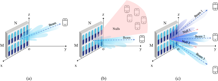
Figure 2: Three common communication scenarios using a MIMO antenna array. (a): Single BF towards the user. (b): Single BF with sidelobe suppression. The red sector covering non-target users represents a wide range of pre-defined nulls. (c): Multiple BF with pre-defined nulls. Generating multiple beams towards several users with nulls to ensure the communication quality.

Each element in the antenna array has several quantized phases. These phases are usually evenly spaced within the range from 0 to 2${\pi}$, and the quantized phase number depends on the encoding precision. If we take the 1-bit encoding technique as an example, the phase of each element will be either 0 or ${\pi}$.

2.2 Binary spin model

Due to phase discretization, BF can be converted to combinatorial optimization problem. For 1-bit and 2-bit encoding, the highest order of spin-spin interaction is 2 and BF is converted to quadratic unconstrained binary optimization (QUBO)[47, 48, 49]. The Ising model, which is important in statistical mechanics describing ferromagnetism[50, 51, 52], is widely used for solving QUBO. It is composed of many spins, each of which has two possible states: spin up (+1) and spin down (-1). These spins are located in a periodic structure, enabling interactions between them[53]. The Hamiltonian of a QUBO problem based on 2D Ising spin model with ${N_{s}}$ spins is shown in Eq. 1, including Ising spins ($s_{i}$, $s_{j}$) and spin-spin interactions ($J_{ij}$):

$$H_{QUBO}={\sum\limits_{i=1}^{N_{s}}{\sum\limits_{j=1}^{N_{s}}{J_{ij}s_{i}s_{j}}}}.$$ (1)

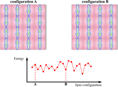
Figure 3: Schematic diagram of Ising model. Ising spins are located in lattices, and the energy of the current state depends on the spin configuration.

It is clear that the energy of the system depends on the spin configuration[54] (see Fig. 3). Although the Ising model is a very powerful tool for solving problems with interactions up to second order, it is ineffective for problems that involve higher-order interactions. In higher-order unconstrained binary optimization (HUBO), we use a general higher-order form of Hamiltonian[55]. For example, the Hamiltonian of the spin model, including interactions between three spins, is shown in Eq. 2:

$$H_{HUBO}={\sum\limits_{i=1}^{N_{s}}{\sum\limits_{j=1}^{N_{s}}{J_{ij}s_{i}s_{j}}}}+{\sum\limits_{i=1}^{N_{s}}{\sum\limits_{j=1}^{N_{s}}{\sum\limits_{p=1}^{N_{s}}{J_{ijp}s_{i}s_{j}s_{p}}}}},$$ (2)

where $J_{ijp}$ = 0 when at least two of $i$, $j$ and $p$ are equal.

The main steps of solving a combinatorial optimization problem can be summarized as follows: Firstly, mapping the variables to be optimized as spins; secondly, defining the objective function of the optimization; thirdly, replacing the variables with spins and substituting them into the objective function. Now, we express the objective function as a Hamiltonian; the last step is to find out the spin configuration minimizing the Hamiltonian.

2.3 Encoding technique

By using an innovative encoding technique, optimizing for specific phase configurations of the antenna array can be converted to a ground state searching problem. In our encoding technique, the phase of each element is represented by polynomials of binary variables with two opposite values ${\pm}$1, corresponding to spin up and spin down. 1-bit encoding[56, 57] is the simplest case, and the phase of each element can be directly expressed as one spin, as shown in Eq. 3:

$$e^{j\psi(m,n)}=s_{p},\leavevmode\nobreak\ p=\left({m-1}\right)N+n.$$ (3)

Here, m and n stand for row index and column index of one antenna element, and $\psi_{mn}$ is the discrete phase of the element (either 0 or $\pi$ in 1-bit encoding). Generally, the 1-bit encoding cannot provide sufficient degrees of freedom to deal with complex BF problems, and the 2-bit encoding was developed[38]. In the 2-bit encoding, there are two spins ($s_{mn1}$ and $s_{mn2}$) in the phase expression of one element. Eq. 4 shows the phase expression, which includes complex coefficients.

$$e^{j\psi(m,n)}=c_{1}s_{p+1}+c_{2}s_{p+2},\leavevmode\nobreak\ p=2\left[{\left({m-1}\right)N+n-1}\right],\ c_{1}=\frac{1+i}{2},\leavevmode\nobreak\ c_{2}=\frac{1-i}{2}.$$ (4)

From the 2-bit encoding, the number of degrees of freedom is increased to cover four different phase values (0, $\frac{\pi}{2}$, $\pi$ and $\frac{3\pi}{2}$). However, conventional encoding techniques (1-bit or 2-bit) are not applicable to achieve higher precision of phase quantization in the phase-only optimization. For example, 16-QAM[58, 59, 60] is a widely used encoding technique with four binary variables employed to compose a constellation including 16 points in the complex plane (shown in Fig. 4(a)).

One can cover at most 8 points sharing the same amplitude in Fig. 4(a); thus, 16-QAM suffers from low efficiency in the phase-only encoding. Here, we propose an efficient technique[61, 62, 63] suitable for high-order encoding. In the proposed technique, we have three variables for the 3-bit encoding, and the phase expression can be written as Eq. 5:

$$e^{j\psi(m,n)}=c_{1}s_{p+1}+c_{2}s_{p+2}+c_{3}s_{p+3}+c_{4}s_{p+1}s_{p+2}s_{p+3},\ p=3\left[{\left({m-1}\right)N+n-1}\right],$$ (5)

where coefficients $c_{1}$, $c_{2}$, $c_{3}$, $c_{4}$ can be calculated from Eq. 6:

$$\textbf{{S}}\textbf{{c}}=\textbf{{p}}$$ , (6)

$$\textbf{{S}}=\begin{bmatrix}1&1&1&1\\ 1&1&-1&-1\\ 1&-1&1&-1\\ 1&-1&-1&1\\ \end{bmatrix} ,\textbf{{c}}=\begin{bmatrix}{\textit{$c_{1}$}}\\ {\textit{$c_{2}$}}\\ {\textit{$c_{3}$}}\\ {\textit{$c_{4}$}}\end{bmatrix},\textbf{{p}}=\begin{bmatrix}0\\ \frac{\pi}{4}\\[4.0pt] \frac{\pi}{2}\\[4.0pt] \frac{3\pi}{4}\end{bmatrix},$$

$$c_{1}=Ae^{j\frac{3\pi}{8}},\leavevmode\nobreak\ c_{2}=Ae^{-j\frac{\pi}{8}} ,\leavevmode\nobreak\ c_{3}=Be^{-j\frac{\pi}{8}},\leavevmode\nobreak\ c_{4}=Be^{-j\frac{5\pi}{8}},$$

$$A=\frac{\sqrt{4+2\sqrt{2}}}{4} ,\leavevmode\nobreak\ B=\frac{\sqrt{4-2\sqrt{2}}}{4}.$$

Here, each row in S corresponds to a spin combination; the first three elements indicate three spins in Eq. 5, and the last element stands for the product of three spins. For example, the first row stands for ${s_{mn1}}$ = 1, ${s_{mn2}}$ = 1, ${s_{mn3}}$ = 1 and the product of them is 1. The connection between phase values p and spins S is given by coefficients c. In the case of 3-bit encoding, the total number of spin combinations should be eight. To ensure Eq. 5 has a unique solution, we select half of them to compose the full-rank matrix S. The remaining four combinations not shown here can be obtained by the negative of one specific row in S, and they are related to the phase values ranging from $\pi$ to $2\pi$. From Fig. 4(b), our encoding ensures every spin combination is mapped onto a point at the unit circle, and it is more suitable for phase-only optimization. The proposed method is also applicable for even higher encoding precision, and a 4-bit encoding technique is provided in the Supplementary Information.

2.4 Objective function

Assuming an $x$-polarized dipole antenna array is placed at the $xoz$ plane, and the normal of the array plane is parallel to the $y$-axis. The source current $\textbf{J}_{\textbf{s}}$ of the dipole is shown in Eq. 7:

$$\mathbf{J}_{\mathbf{s}}=\frac{2}{\eta}e^{jkx{\cos\phi}}\hat{\mathbf{x}},$$ (7)

where $k$ is the wave vector and $\eta$ is the wave impedance.

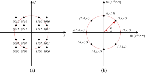
Figure 4: Phase mapping comparison between 16-QAM and our proposed encoding technique. (a): 16-QAM constellation. The circle drawn with a dashed line indicates the points with the same amplitude. (b): Proposed 3-bit encoding. Each point represents a spin combination ($s_{mn1},s_{mn2},s_{mn3}$)

.

Using dyadic Green’s function in electromagnetism, we obtain a far-field radiation pattern of a single element with a size of $d\times d$ based on the source current[64, 38], see Eq. 8:

$$\mathbf{E} =-j\omega\mu\frac{e^{-jkr}}{4\pi r}\left({I+\frac{1}{k^{2}}\nabla\nabla}\right){\int{\mathbf{J}_{\mathbf{s}}\left(\mathbf{r^{\prime}}\right)e^{jk{\hat{\mathbf{r}}\cdot\mathbf{r^{\prime}}}d\mathbf{r^{\prime}}}}},$$ (8)

$$E_{\theta} =-\frac{jkd^{2}}{2\pi r}e^{-jkr}{\cos\theta}\ {\cos\phi}\ \rm{sincX}\ \rm{sincZ},$$

$$E_{\phi} =\frac{jkd^{2}}{2\pi r}e^{-jkr}{\sin\phi}\ \rm{sincX}\ \rm{sincZ},$$

$$X =\frac{kd\ {\sin\theta}\ {\cos\phi}}{2},\ Z=\frac{kd\ {\cos\theta}}{2}.$$

Here $\omega$ is the angular frequency and $\mu$ is the permeability. In BF optimization, the objective function is the total radiated power of the array in the desired direction. For a M $\times$ N array, the array factor can be written as Eq. 9 and the array pattern synthesis is shown in Eq. 10.

$$AF ={\sum\limits_{m=1}^{M}{\sum\limits_{n=1}^{N}{e^{j{({k_{x}md+k_{z}nd})}}e^{j\psi(m,n)}}}},$$ (9)

$$k_{x} =k\ {\sin\theta}\ {\cos\phi},\ k_{z}=k\ {\cos\theta}.$$

The BF Hamiltonian $H_{BF}$ is expressed by the negative of total radiated power within the desired range (solid angle integration centred at the target angle defined by $\theta_{BF}$ and $\phi_{BF}$) as is shown in Eq. 10.

$$H_{BF} =-{\iint{\left|\mathbf{E}\right|^{2}\left|{AF}\right|^{2}}}d\mathbf{\Omega},$$ (10)

$${\iint{d\mathbf{\Omega}}} ={\int_{\phi_{BF}-\frac{\Delta\phi}{2}}^{\phi_{BF}+\frac{\Delta\phi}{2}}{d\phi{\int_{\theta_{BF}-\frac{\Delta\theta}{2}}^{\theta_{BF}+\frac{\Delta\theta}{2}}{{\sin\theta}d\theta}}}}.$$

We take the negative of total radiated power here because the lowest power should be mapped to the best solution for BF optimization. Correspondingly, we use a positive sign for nulls in the desired direction to minimize the radiated power. Furthermore, by substituting Eqs. 3-5 and Eqs. 7-9 into Eq. 10 and equating it to the Hamiltonian in QUBO or HUBO, we obtain the spin-spin interactions and Hamiltonians $J_{pq}$ in 1, 2 and 3-bit encoding (Eqs. 11-16).

$$\ \ \ \ \ \ \ \ \ \ \ \ \ \ \ \ \mathbf{1-bit:}\ J_{pq}=-{\iint{\left|\mathbf{E}\right|^{2}e^{j{[{k_{x}{({m-i})}d+k_{z}{({n-v})}d}]}}d\mathbf{\Omega}}},$$ (11)

$$p=\left({m-1}\right)N+n,\ q=\left({i-1}\right)N+v,$$

where $J_{pq}$ indicates the interaction between the $p^{th}$ spin of the element $(m,n)$ and the $q^{th}$ spin of the element $(i,v)$ in the ${M}\times{N}$ array. In 1-bit encoding, the phase of each element can be simply expressed by a single spin. Therefore, spin-spin interaction only contains one term. The 1-bit Hamiltonian $H^{1-bit}_{BF}$ is shown in Eq. 12:

$$H_{BF}^{1-bit}={\sum\limits_{p=1}^{N_{s}}{\sum\limits_{q=1}^{N_{s}}{J_{pq}s_{p}s_{q}}}},\leavevmode\nobreak\ N_{s}=MN,$$ (12)

where $N_{s}$ is the number of spins.

$$\mathbf{2-bit:}\ J_{pq}=-c_{\alpha}c_{\beta}^{*}{\iint{\left|\mathbf{E}\right|^{2}e^{j{[{k_{x}{({m-i})}d+k_{z}{({n-v})}d}]}}d\mathbf{\Omega}}},$$ (13)

$$p=2\left[{\left({m-1}\right)N+n-1}\right]+\alpha,\ q=2\left[{\left({i-1}\right)N+v-1}\right]+\beta,\ \alpha,\beta\in\left\{1,2\right\},$$

where $c_{\alpha}$ and $c_{\beta}$ are the encoding coefficients in Eq. 4. Here, the spin-spin interactions between two elements consist of four terms, as there are two spins in the phase expression of each element. The 2-bit Hamiltonian $H^{2-bit}_{BF}$ is shown in Eq. 14:

$$H_{BF}^{2-bit}={\sum\limits_{p=1}^{N_{s}}{\sum\limits_{q=1}^{N_{s}}{J_{pq}s_{p}s_{q}}}},\leavevmode\nobreak\ N_{s}=2MN.$$ (14)

In the case of 3-bit encoding, the phase of each element consists of three spins and their product, totalling four terms. As a result, spin-spin interactions between two elements contain 16 terms, which is more complex compared with 2-bit encoding.

$$\mathbf{3-bit:}\ J_{pq}=-c_{\alpha}c_{\beta}^{*}{\iint{\left|\mathbf{E}\right|^{2}e^{j{[{k_{x}{({m-i})}d+k_{z}{({n-v})}d}]}}d\mathbf{\Omega}}},$$ (15)

$$J_{pq}^{Q}=-c_{\alpha}c_{4}^{*}{\iint{\left|\mathbf{E}\right|^{2}e^{j{[{k_{x}{({m-i})}d+k_{z}{({n-v})}d}]}}d\mathbf{\Omega}}},$$

$$J_{pq}^{S}=-\left|c_{4}\right|^{2}{\iint{\left|\mathbf{E}\right|^{2}e^{j{[{k_{x}{({m-i})}d+k_{z}{({n-v})}d}]}}d\mathbf{\Omega}}},$$

$$p=3\left[{\left({m-1}\right)N+n-1}\right]+\alpha,\ q=3\left[{\left({i-1}\right)N+v-1}\right]+\beta,\ \alpha,\beta\in\left\{{1,2,3}\right\},$$

where $c_{\alpha}$ and $c_{\beta}$ can be calculated by Eq. 6. There are three types of spin-spin interactions in 3-bit encoding: quadratic terms (interactions between two spins, $J_{pq}$), quartic terms (interactions between one spin and spin product, $J_{pq}^{Q}$) and six-order terms (interactions between spin products, $J_{pq}^{S}$). Therefore, we obtain the 3-bit Hamiltonian $H^{3-bit}_{BF}$:

$$H_{BF}^{3-bit}= {\sum\limits_{p=1}^{N_{s}}{\sum\limits_{q=1}^{N_{s}}{J_{pq}s_{p}s_{q}}}}+{\sum\limits_{p=1}^{N_{s}}{\sum\limits_{q=1}^{MN}{{J_{pq}^{Q}s}_{p}{\prod\limits_{q^{{}^{\prime}}=3q}^{3q+2}s_{q^{{}^{\prime}}}}}}}+{\sum\limits_{q=1}^{N_{s}}{\sum\limits_{p=1}^{MN}{{J_{qp}^{Q}s}_{q}{\prod\limits_{p^{{}^{\prime}}=3p}^{3p+2}s_{p^{{}^{\prime}}}}}}}$$ (16)

$$+{\sum\limits_{p=1}^{MN}{\sum\limits_{q=1}^{MN}{J_{pq}^{S}{\prod\limits_{p^{{}^{\prime}}=3p}^{3p+2}s_{p^{{}^{\prime}}}}{\prod\limits_{q^{{}^{\prime}}=3q}^{3q+2}s_{q^{{}^{\prime}}}}}}},\leavevmode\nobreak\ N_{s}=3MN.$$

2.5 SB optimizer

Next, the objective Hamiltonian should be embedded into the SB optimizer. SB is an optimization algorithm designed to simulate adiabatic evolutions of classical non-linear Hamiltonian systems with bifurcation phenomena, where two branches of the bifurcation in each non-linear oscillator correspond to two states of each spin[43]. It is based on quantum adiabatic and chaotic evolution theorems and is uniquely suited for parallel computing with its simultaneous updating[44]. This powerful tool is the key to solving large-scale combinatorial optimization problems.

Inspired by the network of Kerr-nonlinear parametric oscillators, the quantum Hamiltonian of BF optimization in this method is defined as[43]:

$$H_{q}(t)=H_{k}(t)+H_{o},$$ (17)

$$H_{k}(t)=\hbar\sum_{i=1}^{N_{s}}\left[\frac{K}{2}a_{i}^{\dagger 2}a_{i}^{2}-\frac{p(t)}{2}\left(a_{i}^{\dagger 2}+a_{i}^{2}\right)+\Delta_{i}a_{i}^{\dagger}a_{i}\right],$$ (18)

$$H_{o}=\hbar\xi_{0}{H_{BF}^{N_{b}-bit}},$$ (19)

where $H_{k}$ represents the Hamiltonian of the Kerr-nonlinear oscillator system and $H_{o}$ represents the Hamiltonian of BF optimization. $N_{s}$ is the number of spins. For the ${M}\times{N}$ array expressed as Eq. 9, $N_{s}$ = ${M}\times{N}\times{N_{b}}$, where ${N_{b}}$ is the number of encoding bits. $\hbar$ represents the reduced Planck constant, $a_{i}^{\dagger}$ and $a_{i}$ denote the creation and annihilation operators for the $i$th oscillator, respectively. The term $K$ stands for the positive Kerr coefficient. The expression $p(t)$ describes the time-dependent amplitude of parametric two-photon pumping. The variable $\Delta_{i}$ indicates the positive detuning frequency, which is the difference between the resonance frequency of the $i$th oscillator and half of the pumping frequency, and $\xi_{0}$ is defined as a positive constant. Here $H_{BF}^{N_{b}-bit}$ is the objective function in Eq. 12, Eq. 14 and Eq. 16. It should be noted that, for 3-bit encoding BF (a HUBO problem), we extend SB algorithm to a general higher-order form[65] instead of using a reduction method[66, 67, 68] to transform a HUBO problem to a QUBO problem, which introduces auxiliary spins and increases computational burden.

Adiabatic evolution theory states that if a system starts in its ground state and the Hamiltonian evolves slowly, the system will stay in the ground state throughout. Initially, each KPO is in a vacuum state. The parameter $\xi_{0}$ is manually chosen small enough to guarantee the vacuum state is the ground state of the initial Hamiltonian. As the pumping strength gradually increases with time, each KPO transitions to a coherent state with a positive or negative amplitude. The final amplitude sign corresponds to the spin in the ground state of the $H_{o}$, as guaranteed by the quantum adiabatic evolution theorem.

Eq. 17 can be transformed to the corresponding classical-mechanical Hamiltonian system to set up the SB optimizer and solve with classical computers. The expectation value of $a_{i}$ is approximated as a complex amplitude $x_{i}+iy_{i}$. $x_{i}$ and $y_{i}$ are a pair of canonical conjugate variables. Thereby, the classical Hamiltonian is derived as follows:

$$H_{c}(\mathbf{x},\mathbf{y},t)=\sum_{i=1}^{N_{s}}\left[\frac{K}{4}\left(x_{i}^{2}+y_{i}^{2}\right)^{2}-\frac{p(t)}{2}\left(x_{i}^{2}-y_{i}^{2}\right)+\frac{\Delta_{i}}{2}\left(x_{i}^{2}+y_{i}^{2}\right)\right]+\frac{\xi_{0}}{2}{H_{BF}^{N_{b}-bit}}.$$ (20)

Since the momentum $\mathbf{y}$ only fluctuates around zero throughout the entire bifurcation process, we neglect fourth-order terms and smaller terms to speed up the calculations and the simplified form of Eq. 20 is derived as follows:

$$H_{\mathrm{SB}}(\mathbf{x},\mathbf{y},t)=\sum_{i=1}^{N_{s}}\frac{\Delta}{2}y_{i}^{2}+V(\mathbf{x},t)=\sum_{i=1}^{N_{s}}\frac{\Delta}{2}y_{i}^{2}+\sum_{i=1}^{N_{s}}\left[\frac{K}{4}x_{i}^{4}+\frac{\Delta-p(t)}{2}x_{i}^{2}\right]+\frac{\xi_{0}}{2}{H_{BF}^{N_{b}-bit}},$$ (21)

where $V(\mathbf{x},t)$ is the potential energy, and all the detunings are set to be the same value $\Delta$. The Eq. 21 is separable with respect to positions and momenta, so we obtain the equation of motion of a particle corresponding to $i^{th}$ spin, as shown in Eq. 22 and Eq. 23[44].

$$\dot{x}_{i}=\frac{\partial H_{\mathrm{SB}}}{\partial y_{i}}=\Delta y_{i},$$ (22)

$$\dot{y}_{i}=-\frac{\partial H_{\mathrm{SB}}}{\partial x_{i}}=-\left[Kx_{i}^{2}-p(t)+\Delta\right]x_{i}-\frac{\xi_{0}}{2}\frac{\partial H_{BF}^{N_{b}-bit}}{\partial x_{i}},$$ (23)

Therefore, we could solve the conjugate variables utilizing the explicit fourth-order Runge-Kutta method[69]. All the variables, $\mathbf{x}$ and $\mathbf{y}$, are initially set around zero. With $p(t)$ gradually increasing from zero, the sign of the final $x_{i}$ represents the $i$th spin, and the final spin configuration should correspond to the ground state. The optimized phase of the MIMO array can be obtained by decoding the obtained spins in the corresponding encoding technique.

In contrast to quantum computers, it’s not necessary to create a physical device based on the quantum Hamiltonian. We can effectively mimic this type of machine using classical computers. Furthermore, the SB optimizer allows one to update variables simultaneously at each time step, therefore allowing acceleration by massively parallel processing. Many parameters need to be carefully chosen in the SB optimizer. Among them, $\xi_{0}$ has the most significant impact on the SB process, which will be explored further in 3.2.2.

3 Results

3.1 Application cases

In this section, we demonstrate several applications of the proposed quantum-inspired algorithm. The total number of antenna elements is 240. We use 1, 2 and 3-bit encoding to map the phase of each element onto spins and calculate spin-spin interaction based on antenna array theory. The SB algorithm solves the spin configuration of the ground state. Three application cases are shown below: single beam, single beam with sidelobe suppression, and multiple beams with nulls. In each example, we plot 1D and 2D far-field patterns, and the radiation patterns are calculated analytically based on array antenna theory.

3.1.1 Single beam

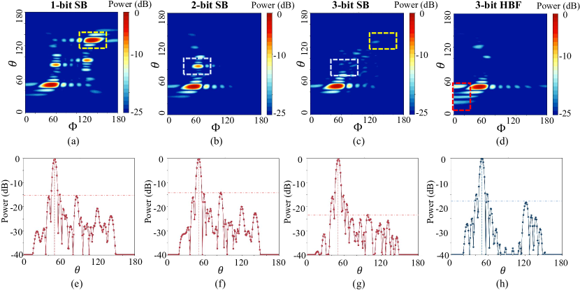
Figure 5: Single BF at $\theta$ = $50^{\circ}$, $\phi$ = $50^{\circ}$ of $10\times 24$ array with different encoding precision by SB and holographic beamforming (HBF) algorithms. (a)-(c): 2D far-field patterns by SB with 1, 2 and 3-bit encoding. (d): 2D far-field patterns by the holographic algorithm with 3-bit encoding. (e)-(g): 1D ($\phi$ = $50^{\circ}$) far-field pattern by SB with 1, 2 and 3-bit encoding. (h): 1D ($\phi$ = $50^{\circ}$) far-field pattern by holographic algorithm with 3-bit encoding.

Single beam is the simplest case and the Hamiltonian $H_{BF}$ is shown in Eq. 10. Considering time-dependent terms in Eq. 17, the quantum Hamiltonian $H_{q}(t)$ of single beamforming is:

$$H_{q}(t)=H_{k}(t)+H_{o}=H_{k}(t)+\hslash\xi_{0}H_{BF}.$$ (24)

The results of single beamforming are shown in Fig. 5. From Fig. 5(a)-(c), we can see that as the encoding precision increases, the radiated power is more concentrated in the desired direction. Notably, due to low phase precision in 1-bit and 2-bit encoding, the flexibility of beamforming is limited, and a high sidelobe is inevitable. The sidelobe is reduced significantly in the case of 3-bit encoding. Comparing Fig. 5(c) with Fig. 5(d), we can see that the SB algorithm performs better than the holographic algorithm[24] (make all elements radiate toward the desired direction, detailed information is provided in Supplementary Information) for the sidelobe suppression (region marked with the red dashed line in Fig. 5(d)).

3.1.2 Single beam with upper sidelobe suppression

In multiple receivers or multiple transmitters scenarios, we need to control the sidelobe in a wide range. In this section, we use a multi-objective function for optimization, including the Hamiltonian of single beam and many sidelobes (see Eq. 25).

$$H_{q}(t) =H_{k}(t)+H_{o}=\left.{H_{k}(t)+\hslash\xi_{0}\left(w\right.}_{0}H_{BF}+H_{nulls}\right),$$ (25)

$$H_{nulls} ={\sum\limits_{i=1}^{N_{nulls}}{w_{i}H}_{null,i}}={\sum\limits_{i=1}^{N_{nulls}}{w_{i}{\iint{\left|\mathbf{E}\right|^{2}\left|{AF}\right|^{2}}}d\mathbf{\Omega}_{i}}},$$

$${\iint{d\mathbf{\Omega}_{i}}} ={\int_{\phi_{i}-\frac{\Delta\phi}{2}}^{\phi_{i}+\frac{\Delta\phi}{2}}{d\phi{\int_{\theta_{i}-\frac{\Delta\theta}{2}}^{\theta_{i}+\frac{\Delta\theta}{2}}{{\sin\theta}d\theta}}}},$$

where $w_{0}$ and $w_{i}$ are the weights of the beamforming Hamiltonian $H_{BF}$ (Eq. 10) and sidelobe suppression Hamiltonian $H_{nulls}$, respectively. The large range of sidelobe suppression is divided into $N_{nulls}$ sub-regions centered at ($\theta_{i}$, $\phi_{i}$). We use a positive sign for each term in $H_{nulls}$ because lower sidelobe levels correspond to lower energy in the objective function. It should be noted that demands like sidelobe suppression in a wide range are beyond the capability of 1-bit and 2-bit schemes. Here, we make a comparison of the performances of the SB and digital BF algorithms with two different BF directions based on 3-bit encoding. In Fig. 6, we plot 1D and 2D far-field patterns optimized by the SB and digital BF. Optimization results at two different BF directions are shown here, and the highest sidelobe level in the 1D far-field pattern is close to -20dB. Besides, a sidelobe level lower than -20dB in a wide range (from $\theta$ = $0^{\circ}$ to $80^{\circ}$) is achieved, and we can see that the SB has a better performance than constrained minimum variance (CMV) optimized digital BF in both sidelobe level and directivity (detailed information of CMV optimized digital BF is provided in Supplementary Information). The directivity of SB in Fig. 6(b) is 597.86, which is higher than that of digital BF in Fig. 6(c) (565.81). In Fig. 6(e), the directivity of SB is 493.69, significantly better than that of digital BF in Fig. 6(f) (328.94).

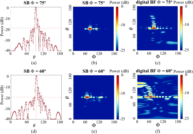
Figure 6: Single BF with sidelobe suppression from $\theta$ = $0^{\circ}$ to $80^{\circ}$ of $10\times 24$ array by SB and digital BF in 3-bit encoding. (a)-(b): 1D ($\phi$ = $75^{\circ}$) and 2D plot of far-field pattern optimized by SB. Beamforming at $\theta$ = $90^{\circ}$, $\phi$ = $75^{\circ}$. (c): 2D plot of far-field optimized by digital BF. Beamforming at $\theta$ = $90^{\circ}$, $\phi$ = $75^{\circ}$. (d)-(e): 1D($\phi$ = $60^{\circ}$) and 2D plot of far-field pattern optimized by SB. Beamforming at $\theta$ = $90^{\circ}$, $\phi$ = $60^{\circ}$. (f): 2D plot of far-field optimized by digital BF. Beamforming at $\theta$ = $90^{\circ}$, $\phi$ = $60^{\circ}$.

3.1.3 Multiple beams with nulls

Multiple beams with pre-defined nulls is another critical application of SB-optimized BF. The capability of generating multiple beams with nulls between them is essential to avoid interference and improve throughput in communication. Apparently, multiple beams require multi-objective optimization (shown in Eq. 26), and we manage to balance the power distribution of these beams by carefully designing the weights of terms in the objective function.

$$H_{q}(t) =H_{k}(t)+H_{o}=H_{k}(t)+\hslash\xi_{0}\left(H_{beams}+H_{nulls}\right),$$ (26)

$$H_{beams} ={\sum\limits_{i=1}^{N_{beams}}{w_{i}H}_{BF,i}}=-w_{i}{\iint{\left|\mathbf{E}\right|^{2}\left|{AF}\right|^{2}}}d\mathbf{\Omega}_{i},$$

where $H_{beams}$ is multi-beamforming Hamiltonian (the number of beams is $N_{beams}$) and $H_{nulls}$ is multi-nulls Hamiltonian (see Eq. 25). We demonstrate the BF optimization with three beams and two predefined nulls between beams. It is clear that SB with 1-bit and 2-bit encoding fails to avoid unwanted beams, and their outputs always show symmetric features limited by encoding precision. While with the proposed 3-bit encoding, SB-based optimization exhibits three beams and nulls lower than -20dB.

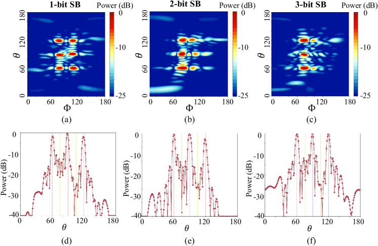
Figure 7: Multiple beams with nulls optimization of $10\times 24$ array by SB with different encoding precision. BF at ($\theta$ = $60^{\circ}$, $\phi$ = $75^{\circ}$), ($\theta$ = $90^{\circ}$, $\phi$ = $75^{\circ}$) and ($\theta$ = $120^{\circ}$, $\phi$ = $75^{\circ}$). Nulls are located at ($\theta$ = $75^{\circ}$, $\phi$ = $75^{\circ}$) and ($\theta$ = $105^{\circ}$, $\phi$ = $75^{\circ}$). (a)-(c): 2D far-field pattern of 1, 2 and 3-bit encoding by SB. (d)-(f): 1D ($\phi$ = $75^{\circ}$) far-field pattern of 1, 2 and 3-bit encoding by SB.

3.2 SB optimizer performance

3.2.1 Parameter settings

The careful selection of parameters significantly influences algorithm convergence. Fortunately, through our exploration, we have developed a set of broadly applicable parameter configurations. We use a linearly increasing time-dependent pumping amplitude $p(t)=0.01t$, as shown in Fig. 8(a). Other parameters are set as $K=1$, $\Delta=0.5$. When $p(t)$ gradually increases from zero to a sufficiently large value, each oscillator exhibits a bifurcation with two stable branches. Fig. 8(b) shows a bifurcation phenomenon optimized at a $5\times 5$ array with a 1-bit encoding. Through brute force validation, the results after the bifurcation found the global optimum.

The step number of iterations significantly affects the solution. For instance, in the case of complex optimization problems (such as the BF with sidelobe suppression in 3.1.2), more iterations are required to achieve a superior solution compared to simple optimization problems (such as the single beam in 3.1.1). Fig. 8(c) shows the optimization process of a $10\times 24$ 3-bit phased array with sidelobe suppression and beamforming at ($\theta$ = $90^{\circ}$, $\phi$ = $60^{\circ}$). Here, we choose different $\xi_{0}$ that corresponds to the optimal solution of each problem. The energy over steps is averaged from multiple experiments and is depicted in the diagram. In the majority of cases, as the number of iterations increases, the energy decreases, indicating the result of a superior solution. At around 1000 steps, the energy reaches convergence, and further increasing the number of steps would lead to significant time consumption without a substantial improvement in solution quality.

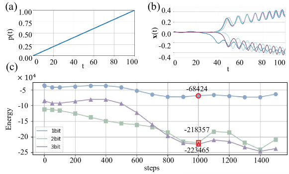
Figure 8: Time-dependent evolution process. (a): Pumping amplitude $p(t)=0.01t$, meeting the requirement of adiabatic approximation condition. (b): bifurcation phenomenon of a $5\times 5$ 1-bit phased array with time increasing. (c): Hamiltonian of a $10\times 24$ 3-bit phased array with sidelobe suppression and BF at ($\theta$ = $90^{\circ}$, $\phi$ = $60^{\circ}$).

At times, the complexity of the problem may lead to an increase in energy when the number of iterations is increased. To strike a balance between solution quality and computational resources, we have opted for 1000 steps as the default iteration count for the optimizer. We could also observe that, in this case, the 2-bit result outperforms the 3-bit result within 800 steps. This is due to the larger search space for 3-bit solutions and the small energy gap between near-ground states and the ground state, which makes 3-bit optimization challenging. However, after surpassing 800 steps and with the use of the SB optimizer, the 3-bit result outperforms the 2-bit result, benefiting from the larger solution space provided by higher bits.

3.2.2 Parameter sensitivity

The parameter $\xi_{0}$ in section 3.2.1 is the only one that cannot be determined. It significantly influences optimizer convergence and solution quality. Observing the sensitivity of the optimizer to $\xi_{0}$ is crucial.

We sampled $\xi_{0}$ from $1\times 10^{-8}$ to 1 with 2000 exponentially spaced samples. The energy distribution for 1 to 3-bit results are illustrated in Fig. 9. Fig. 9(a) shows the energy distribution for the ($\theta$ = $50^{\circ}$, $\phi$ = $50^{\circ}$) single BF (part 3.1.1), Fig. 9(b) displays the result of sidelobe suppression (part 3.1.2) with BF at ($\theta$ = $90^{\circ}$, $\phi$ = $75^{\circ}$), and Fig. 9(c) demonstrates the result of sidelobe suppression (part 3.1.2) with BF at ($\theta$ = $90^{\circ}$, $\phi$ = $60^{\circ}$).

From the perspective of parameter sensitivity, we notice that different problems exhibit varying parameter sensitivities. For simple problems like Fig. 9(a), nearly all $\xi_{0}$ values can find the optimal or near-optimal solution. However, for more complex problems like Fig. 9(b) and Fig. 9(c), the likelihood of finding optimal or near-optimal solutions through an extensive parameter scan decreases significantly. Comparing results with different rank of bit encoding, we observe that the 1-bit solution is much worse than the 2-bit and 3-bit solutions. The 2-bit solution may offer comparable performance to the 3-bit solution with greater stability, but the 3-bit solution can break through the minimum Hamiltonian of the 2-bit solution. These findings corroborate the conclusions drawn in section 3.2.1.

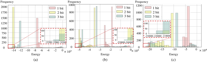
Figure 9: The energy distribution diagram obtained by exponentially sampling 2000 groups of the parameter $\xi_{0}$ between $1\times 10^{-8}$ and 1. (a): case shown in 3.1.1, ($\theta$ = $50^{\circ}$, $\phi$ = $50^{\circ}$) single beam. (b): case shown in 3.1.2, sidelobe suppression with BF at ($\theta$ = $90^{\circ}$, $\phi$ = $75^{\circ}$). (c): case shown in 3.1.2, sidelobe suppression with BF at ($\theta$ = $90^{\circ}$, $\phi$ = $60^{\circ}$).

3.2.3 Parallel efficiency

As pointed out in Part 3.2.2, the choice of $\xi_{0}$ significantly impacts the process of SB, so it’s crucial to select appropriate $\xi_{0}$, which requires a large number of parameter scans. As shown in Fig. 9, out of 2000 sets of parameter scans, although most of the solutions meet the application requirements, the ground state solution is what we ultimately aim for. Thus, we are concerned whether extensive scanning will have a significant impact on solving time. We conducted scans on multiple sets of parameters, and Fig. 10 depicts the relationship between the number of parameter groups and time for 1, 2 and 3-bit encoding.

Figure 10: This diagram shows the solution time of the SB optimizer for different parameter sweep scales. The horizontal axis represents the number of parameter sweep groups, and the vertical axis represents the time taken (in minutes). Time here includes the calculation time of the objective function (Hamiltonians) and the optimization time of the SB optimizer. The line graph shows the total time taken, while the bar graph shows the average time for each parameter. This chart demonstrates the strong parallel performance of the proposed algorithm.

The line chart corresponds to respectively the cases of 1-bit, 2-bit and 3-bit. The solution time does not significantly increase when adding more scanning parameter groups. By analyzing the bar chart, it becomes evident that as the number of scan parameter groups increases, the average time per group decreases. This demonstrates the high parallel efficiency of the SB optimizer. SB enables simultaneous updating of variables at each time step, and the proposed optimizer facilitates the concurrent updates of different sets of variables corresponding to different $\xi_{0}$ at each time step, allowing us to perform a large number of parameter scans at a very low cost. After conducting multiple experiments, we have validated that for a $10\times 24$ array. With a 16-core Intel(R)Core(TM) i7-9700 processor and Python language, the average solution time for the 1-bit optimization problem is 3 seconds, for the 2-bit optimization problem is 12 seconds, and for the 3-bit optimization problem is 50 seconds. As a comparison, genetic algorithms would take several days to complete 300 iterations for the $10\times 24$ array phase optimization problem. This is due to the slow convergence of genetic algorithms, as they update only a portion of the genes during each iteration through the selection, crossover, and mutation operations. The random nature of these operations makes it challenging to obtain the global optimum. Additionally, the performance of genetic algorithms is greatly affected by parameters such as population size, crossover rate, and mutation rate, requiring multiple parameter tuning experiments. In contrast, the SB optimizer outperforms genetic algorithms in terms of iteration process, parameter sensitivity, and solution quality. As the number of groups to be solved increases, the SB optimizer demonstrates a similar overall running time, indicating exceptional performance in parallelization (ideal for fine-tuning parameters).

4 Discussion

In this study, we proposed a quantum-inspired SB algorithm for quantized phase-only massive MIMO BF optimization. A novel encoding technique developed for high-bit phase quantization effectively maps quantized phase values to Ising spins, which are then optimized using the SB optimizer. Our results indicate that the proposed SB optimizer achieves superior performance compared to traditional BF schemes, particularly in handling complex scenarios such as single BF with sidelobe suppression and multiple beams with nulls. When the encoding precision increases from 1-bit to 3-bit, we observe that the energy level structure of the objective Hamiltonian becomes more complex. This complexity increases the likelihood of finding a solution that meets the requirements. However, it also raises the risk of finding a neighboring ground state. The proposed algorithm not only reduces optimization time but also enhances the quality of the optimized solutions. In addition, using the sum of weighted Hamiltonian to describe the optimization objective is a method of constructing an objective function with clearer physical meaning, and it can also be used in other optimization algorithms. These findings open up new opportunities for applying quantum-inspired algorithms to solve other complex optimization problems in wireless communication. This work also possesses additional optimization space. Firstly, the step number of iterations of the SB optimizer is currently fixed at 1000. However, for cases with simple energy level structures of the objective function (such as the single beam case), convergence can be achieved quickly. It would be beneficial to use an adaptive iteration step strategy to determine if the optimization can be stopped based on the convergence of different objective functions. Secondly, apart from $\xi$, other parameters also influence the convergence of the function. For example, the pumping function $p(t)$, the initial Hamiltonian, etc. are factors worth exploring. Future work will explore the extension of this optimizer to higher-bit quantization, GPU acceleration and other challenging applications in BF optimization.

References

- [1] L. Lu, G. Y. Li, A. L. Swindlehurst, A. Ashikhmin, and R. Zhang, “An overview of massive mimo: Benefits and challenges,” IEEE J. Sel. Top. Signal Process., vol. 8, no. 5, pp. 742–758, 2014.
- [2] A. J. Paulraj, D. A. Gore, R. U. Nabar, and H. Bolcskei, “An overview of mimo communications-a key to gigabit wireless,” Proc. IEEE, vol. 92, no. 2, pp. 198–218, 2004.
- [3] J. R. Hampton, Introduction to MIMO communications. Cambridge university press, 2013.
- [4] G. Tsoulos, MIMO system technology for wireless communications. CRC press, 2018.
- [5] A. Goldsmith, S. A. Jafar, N. Jindal, and S. Vishwanath, “Capacity limits of mimo channels,” IEEE J. Sel. Areas Commun., vol. 21, no. 5, pp. 684–702, 2003.
- [6] A. M. Haimovich, R. S. Blum, and L. J. Cimini, “Mimo radar with widely separated antennas,” IEEE Signal Process Mag., vol. 25, no. 1, pp. 116–129, 2007.
- [7] C. Kim, T. Kim, and J.-Y. Seol, “Multi-beam transmission diversity with hybrid beamforming for mimo-ofdm systems,” in 2013 IEEE Globecom Workshops (GC Wkshps). IEEE, 2013, pp. 61–65.
- [8] S. Sun, T. S. Rappaport, R. W. Heath, A. Nix, and S. Rangan, “Mimo for millimeter-wave wireless communications: Beamforming, spatial multiplexing, or both?” IEEE Commun. Mag., vol. 52, no. 12, pp. 110–121, 2014.
- [9] M. N. Kulkarni, A. Ghosh, and J. G. Andrews, “A comparison of mimo techniques in downlink millimeter wave cellular networks with hybrid beamforming,” IEEE Trans. Commun., vol. 64, no. 5, pp. 1952–1967, 2016.
- [10] T. L. Marzetta, “Massive mimo: an introduction,” Bell Labs Tech. J., vol. 20, pp. 11–22, 2015.
- [11] E. G. Larsson, O. Edfors, F. Tufvesson, and T. L. Marzetta, “Massive mimo for next generation wireless systems,” IEEE Commun. Mag., vol. 52, no. 2, pp. 186–195, 2014.
- [12] T. L. Marzetta, E. G. Larsson, and H. Yang, Fundamentals of massive MIMO. Cambridge University Press, 2016.
- [13] E. Björnson, E. G. Larsson, and T. L. Marzetta, “Massive mimo: Ten myths and one critical question,” IEEE Commun. Mag., vol. 54, no. 2, pp. 114–123, 2016.
- [14] A. F. Molisch, V. V. Ratnam, S. Han, Z. Li, S. L. H. Nguyen, L. Li, and K. Haneda, “Hybrid beamforming for massive mimo: A survey,” IEEE Commun. Mag., vol. 55, no. 9, pp. 134–141, 2017.
- [15] E. Ali, M. Ismail, R. Nordin, and N. F. Abdulah, “Beamforming techniques for massive mimo systems in 5g: overview, classification, and trends for future research,” Front. Inf. Technol. Electron. Eng., vol. 18, pp. 753–772, 2017.
- [16] X. Wu, D. Liu, and F. Yin, “Hybrid beamforming for multi-user massive mimo systems,” IEEE Trans. Commun., vol. 66, no. 9, pp. 3879–3891, 2018.
- [17] B. Yang, Z. Yu, J. Lan, R. Zhang, J. Zhou, and W. Hong, “Digital beamforming-based massive mimo transceiver for 5g millimeter-wave communications,” IEEE Trans. Microwave Theory Tech., vol. 66, no. 7, pp. 3403–3418, 2018.
- [18] T. Maksymyuk, J. Gazda, O. Yaremko, and D. Nevinskiy, “Deep learning based massive mimo beamforming for 5g mobile network,” in 2018 IEEE 4th International Symposium on Wireless Systems within the International Conferences on Intelligent Data Acquisition and Advanced Computing Systems (IDAACS-SWS). IEEE, 2018, pp. 241–244.
- [19] R. L. Haupt, “Phase-only adaptive nulling with a genetic algorithm,” IEEE Trans. Antennas Propag., vol. 45, no. 6, pp. 1009–1015, 1997.
- [20] J. F. DeFord and O. P. Gandhi, “Phase-only synthesis of minimum peak sidelobe patterns for linear and planar arrays,” IEEE Trans. Antennas Propag., vol. 36, no. 2, pp. 191–201, 1988.
- [21] A. F. Morabito, A. Massa, P. Rocca, and T. Isernia, “An effective approach to the synthesis of phase-only reconfigurable linear arrays,” IEEE Trans. Antennas Propag., vol. 60, no. 8, pp. 3622–3631, 2012.
- [22] J. Litva and T. K. Lo, Digital beamforming in wireless communications. Artech House, Inc., 1996.
- [23] S. Dutta, C. N. Barati, D. Ramirez, A. Dhananjay, J. F. Buckwalter, and S. Rangan, “A case for digital beamforming at mmwave,” IEEE Trans. Wireless Commun., vol. 19, no. 2, pp. 756–770, 2019.
- [24] E. J. Black, “Holographic beam forming and mimo,” Pivotal Commware, vol. 12, pp. 1–8, 2017.
- [25] R. Deng, B. Di, H. Zhang, Y. Tan, and L. Song, “Reconfigurable holographic surface: Holographic beamforming for metasurface-aided wireless communications,” IEEE Trans. Veh. Technol., vol. 70, no. 6, pp. 6255–6259, 2021.
- [26] H. Guo, B. Makki, and T. Svensson, “A genetic algorithm-based beamforming approach for delay-constrained networks,” in 2017 15th international symposium on modeling and optimization in mobile, ad hoc, and wireless networks (WiOpt). IEEE, 2017, pp. 1–7.
- [27] D. Burgos, J. Kunzler, R. Lemos, and H. Silva, “Adaptive beamforming for moving targets using genetic algorithms,” in 2015 Workshop on Engineering Applications-International Congress on Engineering (WEA). IEEE, 2015, pp. 1–5.
- [28] B. Xia, D. Wang, W. Chen, F. M. Ghannouchi, and Z. Feng, “A 24–40-ghz broadband beamforming trx front-end ic with unified phase and gain control for multiband phased array systems,” IEEE Trans. Very Large Scale Integr. VLSI Syst., 2024.
- [29] T. Suzuki, “L1 generalized inverse beam-forming algorithm resolving coherent/incoherent, distributed and multipole sources,” J. Sound Vib., vol. 330, no. 24, pp. 5835–5851, 2011.
- [30] A. B. Gershman, U. Nickel, and J. F. Bohme, “Adaptive beamforming algorithms with robustness against jammer motion,” IEEE Trans. Signal Process., vol. 45, no. 7, pp. 1878–1885, 1997.
- [31] I. Ahmed, M. K. Shahid, H. Khammari, and M. Masud, “Machine learning based beam selection with low complexity hybrid beamforming design for 5g massive mimo systems,” IEEE Trans. Green Commun. Networking, vol. 5, no. 4, pp. 2160–2173, 2021.
- [32] X. Liu, Y. Liu, and Y. Chen, “Machine learning empowered trajectory and passive beamforming design in uav-ris wireless networks,” IEEE J. Sel. Areas Commun., vol. 39, no. 7, pp. 2042–2055, 2020.
- [33] J. Chen, W. Feng, J. Xing, P. Yang, G. E. Sobelman, D. Lin, and S. Li, “Hybrid beamforming/combining for millimeter wave mimo: A machine learning approach,” IEEE Trans. Veh. Technol., vol. 69, no. 10, pp. 11 353–11 368, 2020.
- [34] N. P. De Leon, K. M. Itoh, D. Kim, K. K. Mehta, T. E. Northup, H. Paik, B. Palmer, N. Samarth, S. Sangtawesin, and D. W. Steuerman, “Materials challenges and opportunities for quantum computing hardware,” Science, vol. 372, no. 6539, p. eabb2823, 2021.
- [35] M. Motta and J. E. Rice, “Emerging quantum computing algorithms for quantum chemistry,” Wiley Interdiscip. Rev.: Comput. Mol. Sci., vol. 12, no. 3, p. e1580, 2022.
- [36] R. D’Cunha, T. D. Crawford, M. Motta, and J. E. Rice, “Challenges in the use of quantum computing hardware-efficient ansatze in electronic structure theory,” J. Phys. Chem. A, vol. 127, no. 15, pp. 3437–3448, 2023.
- [37] J. D. Hidary and J. D. Hidary, Quantum computing: an applied approach. Springer, 2019, vol. 1.
- [38] C. Ross, G. Gradoni, Q. J. Lim, and Z. Peng, “Engineering reflective metasurfaces with ising hamiltonian and quantum annealing,” IEEE Trans. Antennas Propag., vol. 70, no. 4, pp. 2841–2854, 2021.
- [39] J. M. Arrazola, A. Delgado, B. R. Bardhan, and S. Lloyd, “Quantum-inspired algorithms in practice,” Quantum, vol. 4, p. 307, 2020.
- [40] E. Tang, “A quantum-inspired classical algorithm for recommendation systems,” in Proceedings of the 51st annual ACM SIGACT symposium on theory of computing, 2019, pp. 217–228.
- [41] G. Zhang, “Quantum-inspired evolutionary algorithms: a survey and empirical study,” J. Heuristics, vol. 17, no. 3, pp. 303–351, 2011.
- [42] C. Ding, T.-Y. Bao, and H.-L. Huang, “Quantum-inspired support vector machine,” IEEE Trans. Neural Networks Learn. Syst., vol. 33, no. 12, pp. 7210–7222, 2021.
- [43] H. Goto, “Bifurcation-based adiabatic quantum computation with a nonlinear oscillator network,” Sci. Rep., vol. 6, no. 1, p. 21686, 2016.
- [44] H. Goto, K. Tatsumura, and A. R. Dixon, “Combinatorial optimization by simulating adiabatic bifurcations in nonlinear hamiltonian systems,” Sci. Adv., vol. 5, no. 4, p. eaav2372, 2019.
- [45] H. Goto, K. Endo, M. Suzuki, Y. Sakai, T. Kanao, Y. Hamakawa, R. Hidaka, M. Yamasaki, and K. Tatsumura, “High-performance combinatorial optimization based on classical mechanics,” Sci. Adv., vol. 7, no. 6, p. eabe7953, 2021.
- [46] B.-Y. Wang, H. Ge, Y. Jiang, S. S. A. Yuan, T. Chu, Z. Chen, S. Pan, H. Xu, G. Zhang, X. Cui, M.-H. Yung, F. Liu, and W. E. I. Sha, “Quantum-inspired optimization of beamforming with metasurfaces,” in IEEE AP-S/URSI, Portland, Oregon, USA, July 23–28, 2023.
- [47] M. Zaman, K. Tanahashi, and S. Tanaka, “Pyqubo: Python library for mapping combinatorial optimization problems to qubo form,” IEEE Trans. Comput., vol. 71, no. 4, pp. 838–850, 2021.
- [48] F. Glover, G. Kochenberger, and Y. Du, “A tutorial on formulating and using qubo models,” arXiv preprint arXiv:1811.11538, 2018.
- [49] D. Pastorello and E. Blanzieri, “Quantum annealing learning search for solving qubo problems,” Quantum Inf. Process., vol. 18, no. 10, p. 303, 2019.
- [50] S. G. Brush, “History of the lenz-ising model,” Rev. Mod. Phys., vol. 39, no. 4, p. 883, 1967.
- [51] G. F. Newell and E. W. Montroll, “On the theory of the ising model of ferromagnetism,” Rev. Mod. Phys., vol. 25, no. 2, p. 353, 1953.
- [52] R. J. Glauber, “Time-dependent statistics of the ising model,” J. Math. Phys., vol. 4, no. 2, pp. 294–307, 1963.
- [53] T. D. Schultz, D. C. Mattis, and E. H. Lieb, “Two-dimensional ising model as a soluble problem of many fermions,” Rev. Mod. Phys., vol. 36, no. 3, p. 856, 1964.
- [54] J. Dziarmaga, “Dynamics of a quantum phase transition: Exact solution of the quantum ising model,” Phys. Rev. Lett., vol. 95, no. 24, p. 245701, 2005.
- [55] Q. Z. Y. Z. Y. S. M.-H. Y. Bi-Ying Wang, Xiaopeng Cui, “Speedup of high-order unconstrained binary optimization using quantum z2 lattice gauge theory,” arXiv preprint arXiv:2406.05958, 2024.
- [56] H. Kamoda, T. Iwasaki, J. Tsumochi, T. Kuki, and O. Hashimoto, “60-ghz electronically reconfigurable large reflectarray using single-bit phase shifters,” IEEE Trans. Antennas Propag., vol. 59, no. 7, pp. 2524–2531, 2011.
- [57] M.-T. Zhang, S. Gao, Y.-C. Jiao, J.-X. Wan, B.-N. Tian, C.-B. Wu, and A.-J. Farrall, “Design of novel reconfigurable reflectarrays with single-bit phase resolution for ku-band satellite antenna applications,” IEEE Trans. Antennas Propag., vol. 64, no. 5, pp. 1634–1641, 2016.
- [58] P. Dupuis, M. Joindot, A. Leclert, and D. Soufflet, “16 qam modulation for high capacity digital radio system,” IEEE Trans. Commun., vol. 27, no. 12, pp. 1771–1782, 1979.
- [59] C. V. Chong, R. Venkataramani, and V. Tarokh, “A new construction of 16-qam golay complementary sequences,” IEEE Trans. Inf. Theory, vol. 49, no. 11, pp. 2953–2959, 2003.
- [60] M. Kim, D. Venturelli, and K. Jamieson, “Leveraging quantum annealing for large mimo processing in centralized radio access networks,” in Proceedings of the ACM special interest group on data communication, 2019, pp. 241–255.
- [61] Wang, B.-Y.; Cui, X.; Xu, H.; Zhang, G.; Yung, M.-H. Phase encoding method and device. 2024; Patent Application No.CN 202310184040.5.
- [62] Y. Li, X. Cui, Z. Xiong, Z. Zou, B. Liu, B.-Y. Wang, R. Shu, H. Zhu, N. Qiao, and M.-H. Yung, “Efficient molecular conformation generation with quantum-inspired algorithm,” Journal of Molecular Modeling, vol. 30, no. 7, p. 228, 2024.
- [63] Y. Li, X. Cui, Z. Xiong, B. Liu, B.-Y. Wang, R. Shu, N. Qiao, and M.-H. Yung, “Quantum molecular docking with a quantum-inspired algorithm,” Journal of Chemical Theory and Computation, 2024.
- [64] C. A. Balanis, Antenna theory: analysis and design. John wiley & sons, 2016.
- [65] T. Kanao and H. Goto, “Simulated bifurcation for higher-order cost functions,” Appl. Phys. Express, vol. 16, no. 1, p. 014501, 2022.
- [66] R. Xia, T. Bian, and S. Kais, “Electronic structure calculations and the ising hamiltonian,” J. Phys. Chem. B, vol. 122, no. 13, pp. 3384–3395, 2017.
- [67] N. Dattani, “Quadratization in discrete optimization and quantum mechanics,” arXiv preprint arXiv:1901.04405, 2019.
- [68] J. Fujisaki, H. Oshima, S. Sato, and K. Fujii, “Practical and scalable decoder for topological quantum error correction with an ising machine,” Phys. Rev. Res., vol. 4, no. 4, p. 043086, 2022.
- [69] S. Gottlieb and C.-W. Shu, “Total variation diminishing runge-kutta schemes,” Math. Comput., vol. 67, no. 221, pp. 73–85, 1998.