Spacecraft Attitude Control Under Reaction Wheel Constraints Using Control Lyapunov and Control Barrier Functions

Abstract

This paper introduces a novel control strategy for agile spacecraft attitude control, addressing reaction wheel-related input and state constraints. An optimal-decay control Lyapunov function quadratic program stabilizes the system and mitigates chattering at low sampling frequencies, while control barrier functions enforce hard state constraints. Numerical simulations validate the method’s practicality and efficiency for real-time agile spacecraft attitude control.

I Introduction

Agile spacecraft require rapid and precise attitude control to execute critical tasks such as high-resolution imaging and on-orbit servicing. These systems must perform large-angle maneuvers while operating within strict constraints on reaction wheels (RWs) torque and angular momentum. Notable examples include the Pleiades, OrbView, and WorldView satellite systems. [1, 2].

While spacecraft attitude control research is extensive, few studies address RW torque and angular momentum limitations. Methods like sliding mode, backstepping, and adaptive control are known for accuracy and robustness but often fail to handle input or state constraints effectively. We now provide a brief survey of some relevant control approaches.

A classical and efficient approach to handling input constraints is via soft constraints or saturation functions [3, 4]. However, soft constraints require fine-tuning to avoid constraint violations and saturation functions complicate the dynamics and can lead to longer settling times, which is undesirable for rapid maneuvers.

Linearized models have been used in optimization-based methods such as Model Predictive Control (MPC) for spacecraft attitude control [5]. However, spacecraft dynamics’ nonlinearity, especially in large-angle maneuvers, can be problematic. Nonlinear MPC (NMPC) [6] is an alternative, but is computationally intensive, limiting its use in agile spacecraft. MPC-based methods also struggle with robustness against uncertainties and disturbances.

Indirect optimal control computes an optimal policy by solving the Hamilton–Jacobi–Bellman (HJB) equation, but this is done offline and is challenging due to nonlinear dynamics and constraints. Inverse optimal control offers a tractable alternative to solving the HJB equation by identifying a control law with a meaningful cost functional [7]. Control Lyapunov function (CLFs) further simplify solving this problem [7, 8]. Based on Sontag’s formula, this approach has been used for spacecraft attitude control [9], though input constraints are often omitted. CLFs also enable stabilization via point-wise min-norm optimization when formulated as a quadratic program (QP) [10].

CLF-QP-based approaches systematically handle input constraints. A variant, the rapidly exponentially stabilizing CLF (RES-CLF) [11], has been extended to spacecraft attitude control, focusing on input constraints [12]. However, RW angular momentum constraints remain unaddressed. Additionally, CLF-QPs with fixed CLF decay rates (e.g., RES-CLF-QP) may cause input chattering at low sampling frequencies [13, Fig. 6], [14]. While increasing the sampling frequency mitigates this problem, it also increases computational burden, making real-world implementation impractical.

Control Barrier Functions (CBFs) translate state constraints into input constraints, enabling the rigorous study of system safety by ensuring set invariance. CLFs and CBFs can be combined in a QP, where the CLF constraint is slacked to ensure feasibility. This leads to a sequence of QPs solved at each timestep to determine control actions [15].

Zero-order-hold control and robust sampled-data CBFs were used for spacecraft reorientation under pointing and avoid-zone constraints in [16], considering input but not RW angular momentum constraints. A Control Lyapunov-barrier function (CLBF), combining CLFs and CBFs through nonlinear control, was developed in [17] and applied to spacecraft attitude control in [18], but input constraints were not incorporated, and the method faced criticism for theoretical inconsistencies [19].

This paper presents a chatter-free, computationally efficient controller for agile spacecraft attitude stabilization under RW-related input and state constraints. The contributions of this paper are as follows:

1. Unlike previous works on spacecraft attitude control [3, 12], the proposed approach encodes both RW-related input and state constraints as hard constraints via a CLF-CBF-QP controller, offering a computationally efficient alternative to MPC-based methods [6].

2. Unlike prior works that rely on inverse dynamics [13] for the CLF-QP chattering problem, the proposed approach introduces a dynamically varying weight for the CLF decay rate to mitigate the chatter at low sampling frequencies. The controller also balances control effort and settling time through parameter tuning.

3. In prior works, controller designs were typically validated through numerical simulations, which showed absolute performance but did not quantify room for improvement. In our paper, we use a Pareto plot, which visualizes performance trade-offs and compares proposed controllers to a baseline family of optimal policies.

The remainder of the paper is structured as follows: Section II covers relevant preliminaries. Section III outlines the problem statement. Section IV details the controller design. Section V provides comparative simulations, and Section VI concludes the paper with future research directions.

II Preliminaries

Consider a nonlinear input-affine control system

$$\dot{x}=f(x)+g(x)u,\quad y=h(x),$$ (1)

where $x\in\mathbb{R}^{n}$ is the state, $u\in U\subseteq\mathbb{R}^{m}$ is the control input, and $y\in\mathbb{R}^{\ell}$ is the output. In addition, $f:\mathbb{R}^{n}\to\mathbb{R}^{n}$ and $g:\mathbb{R}^{n}\to\mathbb{R}^{n\times m}$ are Lipschitz continuous. We have the following definition for system (1):

Definition 1 (Relative degree [20])

The relative degree of a (sufficiently) differentiable function $h$ with respect to system (1) is the number of times $h$ must be differentiated until the control input $u$ explicitly appears.

II-A Stability via Control Lyapunov Functions (CLF)

Definition 2 (CLF [21])

A continuously differentiable function $V:\mathbb{R}^{n}\to\mathbb{R}$ is a Control Lyapunov Function (CLF) for system (1), if it is positive definite and satisfies

$$\inf_{u\in U}\;\bigl{(}L_{f}V(x)+L_{g}V(x)u\bigr{)}\leq-W(x)\quad\text{for all }x,$$ (2)

where $L_{f}V$ and $L_{g}V$ denote first-order Lie derivatives along $f$ and $g$, respectively and $W$ is a continuous, positive definite function such that $L_{f}V(x)\leq-W(x)$ whenever $L_{g}V(x)=0$. If $V$ is a CLF, define for each $x$ the set
$K_{\textup{CLF}}(x)\colonequals\bigl{\{}u\in U\mid L_{f}V(x)+L_{g}V(x)u\leq-W(x)\bigr{\}}$.

The function $W$ represents the desired decay rate of the closed-loop $\dot{V}$, with different choices for $W$ leading to different inverse optimal control laws [21].

Theorem 1 (See [21])

For system (1), if there exists a CLF $V:\mathbb{R}^{n}\to\mathbb{R}$, i.e., a positive definite function satisfying (2), then any Lipschitz continuous controller $u$ satisfying $u(x)\in K_{\textup{CLF}}(x)$ for all $x\in\mathbb{R}^{n}$ asymptotically stabilizes the system to the origin.

II-B Safety via Control Barrier Functions (CBF)

Definition 3 (CBF [20])

Let $\mathcal{C}$ be the superlevel set of a continuously differentiable function $B:\mathbb{R}^{n}\to\mathbb{R}$, so that $\mathcal{C}=\{x\in\mathbb{R}^{n}\;|\;B(x)\geq 0\}$. $B$ is a Control Barrier Function (CBF) for system (1) if there exists $\alpha\geq 0$ such that

$$\sup_{u\in U}\;\bigl{(}L_{f}B(x)+L_{g}B(x)u\bigr{)}\geq-\alpha B(x)\quad\text{for all }x\in\mathcal{C}.$$ (3)

If $B$ is a CBF, define for each $x\in\mathcal{C}$ the set
$K_{\textup{CBF}}(x)\colonequals\bigl{\{}u\in U\;\mid\;L_{f}B(x)+L_{g}B(x)u\geq-\alpha B(x)\bigr{\}}$.

Theorem 2 (See [20, 15])

Let $\mathcal{C}$ be defined as in Definition 3. If $B$ is a CBF for system (1), then any Lipschitz continuous controller $u(x)\in K_{\textup{CBF}}(x)$ has the property that if $x(0)\in\mathcal{C}$, then $x(t)\in\mathcal{C}$ for all $t\geq 0$.

The property of $\mathcal{C}$ in Theorem 2 is also called forward invariance [22].

III Problem Statement

III-A Spacecraft Attitude Model

For simplicity, we assume three identical, axially symmetric RWs aligned with the spacecraft’s principal axes. This ensures the wheel rotations do not affect the system’s moment of inertia. The angular momentum of the RWs $h_{w}$ is calculated as $h_{w}=J_{w}\omega_{w}$, where $J_{w}=\operatorname{diag}(J_{w1},J_{w2},J_{w3})$, and $\omega_{w}\in\mathbb{R}^{3}$ are the RWs moment of inertia and angular velocity, respectively. In this formulation, the spacecraft’s angular velocity contribution to the RWs’ angular momentum is neglected because it is small compared to the RWs’ angular velocity. Although the RWs’ angular velocity can be large, it is always bounded, ensuring that $h_{w}$ also remains bounded [1].

Attitude dynamics are given by the equations [23]

$$\dot{\sigma} =M(\sigma)\omega,$$ (4a)

$$J\dot{\omega} =-{\omega}^{\times}(J\omega+h_{w})+u+d,$$ (4b)

$$\dot{h}_{w} =-u,$$ (4c)

where $\sigma\in\mathbb{R}^{3}$ is the attitude representation using Modified Rodrigues Parameters (MRPs), $J\in\mathbb{R}^{3\times 3}$ and $\omega\in\mathbb{R}^{3}$ are the inertia matrix and angular velocity of the spacecraft, expressed in the body-fixed frame, $d\in\mathbb{R}^{3}$ is the external disturbance torque and $u\in\mathbb{R}^{3}$ is the control torque. The notation ${x}^{\times}\in\mathbb{R}^{3\times 3}$ denotes the cross-product matrix operator. Additionally, $M(\sigma)\colonequals\frac{1}{4}\bigl{(}(1-{\sigma}^{\mathsf{T}}\sigma)I_{3}+2{\sigma}^{\times}+2\sigma{\sigma}^{\mathsf{T}}\bigr{)}$. Eq. 4a captures the kinematics and (4b) and (4c) describe the spacecraft and RWs dynamics, respectively.

With the state vector defined as $x={\begin{bmatrix}{\sigma}^{\mathsf{T}}&{\omega}^{\mathsf{T}}&{h}^{\mathsf{T}}_{w}\end{bmatrix}}^{\mathsf{T}}$ and external disturbances neglected, the dynamics (4) can be written in input-affine form (1), with

$$f(x)\colonequals\begin{bmatrix}M(\sigma)\omega\\ -J^{-1}{\omega}^{\times}(J\omega+h_{w})\\ 0_{3\times 1}\end{bmatrix}\!,\;g(x)\colonequals\begin{bmatrix}0_{3\times 3}\\ J^{-1}\\ -I_{3}\end{bmatrix}\!.$$ (5)

Remark 1

In this paper, we consider a rest-to-rest maneuvers where $x(0)={\begin{bmatrix}{\sigma_{0}}^{\mathsf{T}}&{0}^{\mathsf{T}}&{0}^{\mathsf{T}}\end{bmatrix}}^{\mathsf{T}}$ and $x_{\textup{final}}=0$. If the final state is nonzero, then instead of (5), we should use the so-called relative error equations [23].

IV Controller Design

In this section, we design a stabilizing controller based on the CLF formulation (2). We then discuss how formulating the CLF with a fixed decay rate in a QP can cause input chattering at low sampling frequencies and propose a fix. Finally, we encode the RWs angular momentum constraint (state constraint) using the CBF concept (3) and formulate a CLF-CBF-QP for the spacecraft attitude control system (4).

IV-A CLF-QP Design

We begin by summarizing the input-output linearization procedure and applying it to the spacecraft attitude dynamics to form a quadratic CLF. While the focus of this paper is on spacecraft attitude control, the formulations in this subsection can be used to design a CLF for a general nonlinear input-affine dynamical system. If the system (1) has relative degree $r$, and $\ell=m$, then we have

$$y^{(r)}=L_{f}^{r}h(x)+L_{g}L_{f}^{r-1}h(x)u,$$ (6)

where $L_{f}^{r}h(x)$ and $L_{g}L_{f}^{r-1}h(x)$ are the $r^{\text{th}}$ order Lie derivatives, and $y^{(r)}$ is the $r^{\text{th}}$ time derivative of $y$. If $L_{g}L_{f}^{r-1}h(x)\in\mathbb{R}^{m\times m}$ is nonsingular for all $x\in\mathbb{R}^{n}$, then we can apply a control input that renders the input-output dynamics of the system linear:

$$u(x,\mu)=u^{*}(x)+(L_{g}L_{f}^{r-1}h(x))^{-1}\mu,$$ (7)

where $u^{*}(x)\colonequals-(L_{g}L_{f}^{r-1}h(x))^{-1}L_{f}^{r}h(x)$ is the feedforward term and $\mu\in\mathbb{R}^{m}$ is the auxiliary input. Using this control law yields the input-output linearized system $y^{(r)}=\mu$, and we can define a state transformation $x\mapsto(\eta,z)$, with the transverse coordinates $\eta\colonequals{\begin{bmatrix}{h(x)}^{\mathsf{T}}&{L_{f}h(x)}^{\mathsf{T}}&\cdots&{L_{f}^{r-1}h(x)}^{\mathsf{T}}\end{bmatrix}}^{\mathsf{T}}$ and the zero-dynamics manifold $z\in\{x\in\mathbb{R}^{n}\;|\;\eta=0\}$. The closed-loop dynamics of the system can then be represented as a linear time-invariant system on $\eta$ and $z$:

$$\dot{\eta}=F\eta+G\mu,\quad\dot{z}=p(\eta,z),$$ (8)

where $F\!=\!\begin{bmatrix}0&1&\cdots&0\\ \vdots&\vdots&\ddots&\vdots\\ 0&0&\cdots&1\\ 0&0&\cdots&0\end{bmatrix}\otimes I_{m}$, $G\!=\!\begin{bmatrix}0\\ \vdots\\ 0\\ 1\end{bmatrix}\otimes I_{m}$, and $F\in\mathbb{R}^{mr\times mr}$, $G\in\mathbb{R}^{mr\times m}$, and $\otimes$ is the Kronecker product.

It can be verified that $V(\eta)={\eta}^{\mathsf{T}}P\eta$ is a CLF for the input-output linearized system (8). Defining $\bar{f}\colonequals F\eta$, $\bar{g}\colonequals G$, we have: $\dot{V}(\eta,\mu)=L_{\bar{f}}V(\eta)+L_{\bar{g}}V(\eta)\mu$, where $L_{\bar{f}}V(\eta)={\eta}^{\mathsf{T}}({F}^{\mathsf{T}}P+PF)\eta$ and $L_{\bar{g}}V(\eta)=2{\eta}^{\mathsf{T}}PG$. Now consider the following quadratic cost:

$$J=\int_{0}^{\infty}\bigl{(}{{\eta}^{\mathsf{T}}Q\eta}+{u}^{\mathsf{T}}\bar{R}u\bigr{)}\,\mathrm{d}t,$$ (9)

where $Q\in\mathbb{R}^{mr\times mr}$, $\bar{R}=\nu I_{m}\in\mathbb{R}^{m\times m}$ and $\nu$ is a design variable to penalize the input usage for the initial nonlinear system. Let $\bar{L}\colonequals L_{g}L_{f}^{r-1}h(x)$ and $\bar{\mu}\colonequals L_{f}^{r}h(x)$. Since the input of the linearized system is $\mu$, we can rewrite (9) as

$$J=\int_{0}^{\infty}\Bigl{(}{\eta}^{\mathsf{T}}Q\eta+{(\mu-\bar{\mu})}^{\mathsf{T}}R(\mu-\bar{\mu})\Bigr{)}\,\mathrm{d}t,$$ (10)

where $R\colonequals\bar{L}^{-\mathsf{T}}\bar{R}\bar{L}^{-1}=\nu(\bar{L}^{-\mathsf{T}}\bar{L}^{-1})\in\mathbb{R}^{m\times m}$. Under standard stabilizability and detectability assumptions, there is a unique symmetric positive definite solution $P$ to the continuous-time algebraic Riccati equation

$${F}^{\mathsf{T}}P+PF+Q-PGR^{-1}{G}^{\mathsf{T}}P=0.$$ (11)

Now consider (2). If we choose $W(\eta)$ as

$$W(\eta)=\sqrt{(L_{\bar{f}}V(\eta))^{2}+({\eta}^{\mathsf{T}}Q\eta)(L_{\bar{g}}V(\eta))R^{-1}{(L_{\bar{g}}V(\eta))}^{\mathsf{T}}}$$

$$=\sqrt{({\eta}^{\mathsf{T}}({F}^{\mathsf{T}}P+PF)\eta)^{2}+4({\eta}^{\mathsf{T}}Q\eta)({\eta}^{\mathsf{T}}PGR^{-1}{G}^{\mathsf{T}}P\eta)}$$

$$={\eta}^{\mathsf{T}}(Q+PGR^{-1}{G}^{\mathsf{T}}P)\eta,$$ (12)

then the QP based on this formula recovers the standard Linear Quadratic (LQ) optimal control law $\mu=-R^{-1}{G}^{\mathsf{T}}P\eta$ when the system dynamics are linear, and produces an efficiently computable control strategy when the system is nonlinear and feedback linearizable [10].

For our spacecraft attitude control problem, we choose the output $y=h(x)=\sigma$. With this choice, the system has a relative degree of $r=2$, giving $\eta={\begin{bmatrix}{\sigma}^{\mathsf{T}}&{\dot{\sigma}}^{\mathsf{T}}\end{bmatrix}}^{\mathsf{T}}$.

Remark 2

The zero dynamics for the spacecraft attitude control problem exist and are stable. For details, see [24].

IV-B Addressing Input Chattering

The CLF-QP formulation based on (2) with (IV-A) forms a point-wise min-norm optimization problem ensuring system stability per Theorem 1. However, solving this QP at low sampling frequencies can cause input chattering [14], due to the fixed CLF decay rate generating aggressive control signals to maintain stability over longer intervals between updates.

In [25], a variable decay weight was introduced for the CBF to ensure the feasibility of the CBF and input constraints in a CBF-QP. Inspired by this, we introduce the variable decay weight $\rho\in[0,1]$ for the decay rate of the CLF in (2) as:

$$\inf_{u\in U}\;\bigl{(}L_{f}V(x)+L_{g}V(x)u\bigr{)}\leq-\rho W(x).$$ (13)

We include $\rho$ in the QP as an extra decision variable, which dynamically adjusts the decay rate of the CLF to balance stabilization speed with input smoothness. By varying the decay rate, we prevent aggressive corrections that cause chattering, ensuring smoother inputs without compromising stability.

Remark 3

In (IV-A), if $R=I$, an alternative choice is

$$W(\eta)=\frac{1}{\varepsilon}\frac{\lambda_{\min}(Q)}{\lambda_{\max}(P)}V(\eta),$$ (14)

where $\lambda_{\min}$ and $\lambda_{\max}$ denote minimum and maximum eigenvalues and $\varepsilon$ is a design variable. This formulation, termed RES-CLF, was first introduced in [11]. While the variable $\varepsilon$ adjusts the decay rate of the RES-CLF, manually tuning it to achieve the optimal settling time without inducing chattering is challenging. Adding a variable decay weight as described above can also help control chattering with a RES-CLF.

IV-C CLF-CBF-QP Design

We now apply the CBF concept to encode box constraints on the RW angular momentum. The constraints are given by $\underaccent{\bar}{h}_{w}\leq h_{w}\leq\bar{h}_{w}$, where $\underaccent{\bar}{h}_{w}\colonequals h_{w,\min}{\begin{bmatrix}1&1&1\end{bmatrix}}^{\mathsf{T}}$ and $\bar{h}_{w}\colonequals h_{w,\max}{\begin{bmatrix}1&1&1\end{bmatrix}}^{\mathsf{T}}$. Define the vector-valued CBFs $\underaccent{\bar}{B}(x)\colonequals h_{w}-\underaccent{\bar}{h}_{w}$ and $\bar{B}(x)\colonequals\bar{h}_{w}-h_{w}$. These CBFs encode the minimum and maximum angular momentum constraints for each RW, respectively.

The Jacobian matrices for these CBFs are given by $\nabla\underaccent{\bar}{B}(x)=-\nabla\bar{B}(x)={\begin{bmatrix}0_{3\times 3}&0_{3\times 3}&I_{3}\end{bmatrix}}^{\mathsf{T}}$. Therefore, the Lie derivatives with respect to the spacecraft dynamics (5) are $L_{f}\underaccent{\bar}{B}(x)=L_{f}\bar{B}(x)=0_{3\times 1}$ and $L_{g}\underaccent{\bar}{B}(x)=-L_{g}\bar{B}(x)=-I_{3}$. The CBF constraints $L_{f}\underaccent{\bar}{B}(x)+L_{g}\underaccent{\bar}{B}(x)u\geq-\alpha\underaccent{\bar}{B}(x)$ and $L_{f}\bar{B}(x)+L_{g}\bar{B}(x)u\geq-\alpha\bar{B}(x)$ can therefore be expressed succinctly as $-\alpha\bar{B}(x)\leq u\leq\alpha\underaccent{\bar}{B}(x)$.

Putting everything together, we obtain our proposed Optimal-Decay CLF-CBF-QP (OD-CLF-CBF-QP):

$$\underset{u,\rho,\delta}{\min}\quad \left\|\bar{L}(u-u^{*})\right\|_{H}^{2}+p_{\rho}(1-\rho)^{2}+p_{\delta}\delta^{2}$$ (15)

s.t. $$L_{\bar{f}}V(\eta)+L_{\bar{g}}V(\eta)\bar{L}(u-u^{*})\leq-\rho W(\eta)+\delta,$$

$$-\alpha\bar{B}(x)\leq u\leq\alpha\underaccent{\bar}{B}(x),\;\underaccent{\bar}{u}\leq u\leq\bar{u},\;\rho\geq 0,$$

where $H\succ 0$ is a weighting matrix and $\|x\|_{H}^{2}\colonequals{x}^{\mathsf{T}}Hx$. Our formulation (15) includes a weight $p_{\delta}>0$ for the slack variable $\delta\in\mathbb{R}$, which ensures the CLF constraint is always feasible. The weight $p_{\rho}>0$ penalizes the variable decay weight $\rho\geq 0$ and we use an associated cost $(1-\rho)^{2}$ to favor $\rho=1$ (the nominal decay weight). The input torque bounds are $\underaccent{\bar}{u}=u_{\min}{\begin{bmatrix}1&1&1\end{bmatrix}}^{\mathsf{T}}$ and $\bar{u}=u_{\max}{\begin{bmatrix}1&1&1\end{bmatrix}}^{\mathsf{T}}$.

Our OD-CLF-CBF-QP (15) is always feasible due to the slack variable $\delta$ (e.g., let $u=0$), and guarantees safety (state and input constraints are never be violated) for the spacecraft due to Theorem 2. Asymptotic stability (that we eventually reach our goal of $x=0$) is not guaranteed, but we can monitor $\delta$ in real-time and whenever $\delta=0$, we are assured by Theorem 1 that the state is approaching the desired goal $x\to 0$. The main ways we tune our controller are:

• Varying the CBF decay rate $\alpha>0$. Increasing $\alpha$ means the controller will be more aggressive and allow itself to get closer to state constraint boundaries.

• Varying the input penalty $\nu$ in (9). Increasing $\nu$ results in using less input and favors slower maneuvers.

V Simulation and Results

In this section, we provide an empirical evaluation of our controller and compare its performance to that of alternative control strategies, including an optimal control strategy. The simulation parameters we used are given in Table I.

TABLE I: Simulation Parameters

Inertia Matrix	$\mathbf{J}=\bigg{[}\begin{smallmatrix}1.8140&-0.1185&0.0275\\ -0.1185&1.7350&0.0169\\ 0.0275&0.0169&3.4320\end{smallmatrix}\bigg{]}\,\unit{kg.m^{2}}$
RWs Torque Limits	$u_{\max}=-u_{\min}=\qty{0.123}{N.m}$
RWs Momentum Limits	$h_{w,\max}=-h_{w,\min}=\qty{0.50}{N.m.s}$
Initial Euler Angles (3-2-1)	$\psi_{0}={\begin{bmatrix}$$&$$&$$\end{bmatrix}}^{\mathsf{T}}$
Initial Angular Velocities	$\omega_{0}={\begin{bmatrix}0&0&0\end{bmatrix}}^{\mathsf{T}}\,\unit{rad/s}$
Sampling Frequency	10Hz (QP solves per second)

V-A Optimal Control Simulations

This subsection formulates a family of optimal control problems as a baseline for comparison with the proposed OD-CLF-CBF-QP (15). For different final times $T_{\text{final}}\in(0,100]$, we solved the nonlinear energy-optimal control problem (OCP) in (16), establishing a Pareto Optimal Curve that trades off control effort and total maneuver time. For OCP simulations, we used the Python Control Systems Library [26], which implements a direct discretize-then-optimize approach using the SLSQP solver to obtain an open-loop optimal trajectory. For our proposed OD-CLF-CBF-QP and all other QP-based controllers, we used CVXPY with the PROXQP solver [27]. All simulations were conducted on an Apple M2 Pro chip with 32GB of RAM.

The energy-optimal control problem (OCP) is given by

$$\underset{u}{\min}\quad \int_{0}^{T_{\text{final}}}\|u\|_{H}^{2}\,\mathrm{d}t$$ (16)

s.t. $$\dot{x}=f(x)+g(x)u,$$

$$x(0)=x_{0},\;x(T_{\text{final}})\in\mathcal{T},$$

$$\underaccent{\bar}{h}_{w}\leq h_{w}\leq\bar{h}_{w},\;\;\underaccent{\bar}{u}\leq u\leq\bar{u},$$

where $x={\begin{bmatrix}{\sigma}^{\mathsf{T}}&{\omega}^{\mathsf{T}}&{h_{w}}^{\mathsf{T}}\end{bmatrix}}^{\mathsf{T}}$ and $H=I_{3}$. We used the terminal set $\mathcal{T}=\left\{x\;\middle|\;\|\sigma\|_{\infty}\leq 0.02\text{ and }\|\omega\|_{\infty}\leq 0.005\right\}$. For QP-based controllers, since we cannot explicitly specify the final time, we ran the controller for a long time and then computed $T_{\text{final}}$ post hoc using

$$T_{\text{final}}=\inf\left\{t\geq 0\;\middle|\;x(\tau)\in\mathcal{T}\text{ for all }\tau\geq t\right\}.$$

Results are shown in Fig. 1. The OCP curve serves as a lower bound indicating the most efficient possible maneuver for a given $T_{\text{final}}$. Meanwhile, the max control effort line (using $u(t)=u_{\text{max}}$ for all $t\geq 0$), serves as an upper bound.

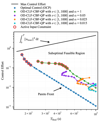
Figure 1: The Pareto curve, derived from solving the OCP (16) for various final times, is compared to the proposed OD-CLF-CBF-QP (15) across different tunings of $\nu$ and $\alpha$, with log-scaled $x$-$y$ axes.

In Fig. 1, we show a variety of tunings of $\nu$ and $\alpha$ for our proposed OD-CLF-CBF-QP to illustrate the trade-off between input energy and total maneuver time. Increasing $\nu$ (input penalty) favors slower maneuvers by using less input. Likewise, increasing $\alpha$ (CBF decay rate) allows trajectories to get closer to state constraint boundaries, resulting in faster maneuvers. Each tuning is guaranteed to produce feasible QPs and safe trajectories. As we tune the controller, we obtain performances that trace out a trade-off curve roughly parallel to the OCP curve, indicating that control effort is roughly a constant factor worse than optimal.

V-B Comparative Simulations

We now compare five controllers, again with the simulation parameters from Table I. Each controller was tuned manually to achieve good performance and comparable $T_{\text{final}}$.

1. PD controller with saturation, using $k_{p}=0.4$, $k_{d}=0.8$. This controller does not require solving a QP.

2. RES-CLF-QP [11, 12], using $Q=I_{6}$, $K_{1}=0.01\cdot I_{3}$, $K_{2}=0.05\cdot I_{3}$, $\varepsilon=0.2$, $H=I_{3}$, and $p_{\delta}=100$.

3. OD-CLF-QP, which is the same as our proposed OD-CLF-CBF-QP controller (15), but without the CBF constraint $-\alpha\bar{B}(x)\leq u\leq\alpha\underaccent{\bar}{B}(x)$. We used $p_{\rho}=0.1$, $\nu=10$, and the same $H$, $p_{\delta}$, and $Q$ as in Item 2.

4. Our proposed OD-CLF-CBF-QP controller (15), tuned using the parameters of Item 3 and $\alpha=0.05$.

5. OCP (16). We chose $T_{\text{final}}$ to match the other controllers. We plotted open-loop performance to serve as a “best possible” comparative benchmark.

We note that controllers 1–3 satisfy the input constraints, but cannot guarantee that state constraints (e.g., the RW constraint on $h_{w}$) will be satisfied. Resulting state and input trajectories are shown in Fig. 2, the evolution of decay weights and slack variables in Fig. 3, and a comparison of wall clock time is given in Table II.

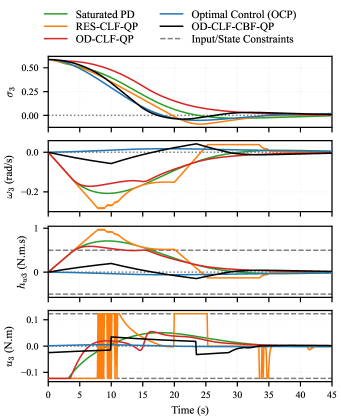
Figure 2: Attitude MRPs, angular velocity, RW angular momentum, and control torque simulation responses for various controllers. Only the 3^rd components of $\sigma$, $\omega$, $h_{w}$, and $u$ are plotted in the interest of space. The other components look similar.

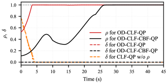
Figure 3: Optimal decay weight $\rho$ and slack variable $\delta$ simulation response for OD-CLF-QP, and OD-CLF-CBF-QP. Since $\delta\to 0$, we are assured that the trajectory is asymptotically stable.

TABLE II: Wall clock time comparison for different controllers. The corresponding state and input trajectories are shown in Fig. 2.

	Control Method	Wall Clock Time	Cost $\int_{0}^{T}\|u\|^{2}\,\mathrm{d}t$
1.	Saturated PD	$\qty{0.12}{sec}$	$0.1892$
2.	RES-CLF-QP	$\qty{1.44}{sec}$	$0.8002$
3.	OD-CLF-QP	$\qty{1.92}{sec}$	$0.1744$
4.	OD-CLF-CBF-QP	$\qty{2.09}{sec}$	$0.0430$
5.	Optimal Control (OCP)	$\qty{17.2}{sec}$	$0.0130$

Fig. 2 shows that all controllers successfully perform rest-to-rest maneuvers despite large initial angles. The RES-CLF-QP experiences input chattering, while the OD-CLF-QP and OD-CLF-CBF-QP maintain smooth performance due to the varying decay weight $\rho$ (Fig. 3) described in Section IV-B. Chatter can also be eliminated by increasing the sampling rate, but this increases computational burden.

The Saturated PD, RES-CLF-QP, and OD-CLF-QP, which lack the ability to enforce state constraints, fail to satisfy the RW angular momentum limits (see $h_{w3}$ plot in Fig. 2).

As shown in Table II, the proposed OD-CLF-CBF-QP achieves a cost comparable to the OCP while offering significant computational time savings. Controllers 2–4 each solve the same number of QPs, but OD-CLF-CBF-QP takes slightly longer since its associated QP has an additional CBF constraint and decision variable $\rho$.

V-C Monte Carlo Simulations

We ran Monte Carlo simulations with 20 random initial orientations (uniformly distributed on a sphere) to demonstrate the effectiveness of the proposed OD-CLF-CBF-QP controller (15). We used the same control parameters as in Section V-B, except we set $\alpha=1$ to allow the trajectories to approach the state constraints more closely.

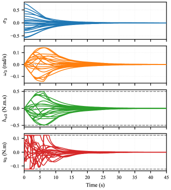
Figure 4: Simulated state and input responses for the OD-CLF-CBF-QP controller for 20 randomized initial orientations. Only the 3^rd components of $\sigma$, $\omega$, $h_{w}$, $u$ are plotted in the interest of space; the rest look similar.

The simulation results, shown in Fig. 4, verify that the proposed OD-CLF-CBF-QP effectively performs safe rest-to-rest maneuvers with random large initial states while avoiding input chatter.

VI Conclusion

We proposed a control strategy for agile spacecraft attitude control using control barrier functions (CBF) and quadratic programming (QP) to address reaction wheel torque and angular momentum constraints. The approach introduces a dynamic optimal-decay weight for the control Lyapunov function (CLF) to reduce chattering at low sampling frequencies while balancing control effort and settling time.

References

- [1] X. Cao, C. Yue, M. Liu, and B. Wu, “Time efficient spacecraft maneuver using constrained torque distribution,” Acta Astronautica, vol. 123, pp. 320–329, 2016.
- [2] F. L. Markley, R. G. Reynolds, F. X. Liu, and K. L. Lebsock, “Maximum torque and momentum envelopes for reaction wheel arrays,” Jour. Guid. Control Dyn., vol. 33, no. 5, pp. 1606–1614, 2010.
- [3] M. Alipour, M. Malekzadeh, and A. Ariaei, “Practical fractional-order nonsingular terminal sliding mode control of spacecraft,” ISA Transactions, vol. 128, pp. 162–173, 2022.
- [4] A.-M. Zou and K. D. Kumar, “Finite-time attitude control for rigid spacecraft subject to actuator saturation,” Nonlinear Dynamics, vol. 96, pp. 1017–1035, 2019.
- [5] C. Zagaris, H. Park, J. Virgili-Llop, R. Zappulla, M. Romano, and I. Kolmanovsky, “Model predictive control of spacecraft relative motion with convexified keep-out-zone constraints,” Jour. Guid. Control Dyn., vol. 41, no. 9, pp. 2054–2062, 2018.
- [6] D. Y. Lee, R. Gupta, U. V. Kalabić, S. Di Cairano, A. M. Bloch, J. W. Cutler, and I. V. Kolmanovsky, “Geometric mechanics based nonlinear model predictive spacecraft attitude control with reaction wheels,” Jour. Guid. Control Dyn., vol. 40, no. 2, pp. 309–319, 2017.
- [7] M. Krstic and Z.-H. Li, “Inverse optimal design of input-to-state stabilizing nonlinear controllers,” IEEE Trans. Autom. Control, vol. 43, pp. 336–350, 1998.
- [8] W. Luo, Y.-C. Chu, and K.-V. Ling, “Inverse optimal adaptive control for attitude tracking of spacecraft,” IEEE Trans. Autom. Control, vol. 50, pp. 1639–1654, 2005.
- [9] C. Pukdeboon and A. S. I. Zinober, “Control Lyapunov function optimal sliding mode controllers for attitude tracking of spacecraft,” Journal of the Franklin Institute, vol. 349, no. 2, pp. 456–475, 2012.
- [10] R. A. Freeman and P. V. Kokotovic, “Optimal nonlinear controllers for feedback linearizable systems,” in Amer. Control Conf., vol. 4, 1995, pp. 2722–2726.
- [11] A. D. Ames, K. Galloway, K. Sreenath, and J. W. Grizzle, “Rapidly exponentially stabilizing control Lyapunov functions and hybrid zero dynamics,” IEEE Trans. Autom. Control, vol. 59, no. 4, pp. 876–891, 2014.
- [12] B. Li, Q. Hu, and G. Ma, “Extended state observer based robust attitude control of spacecraft with input saturation,” Aerospace Science and Technology, vol. 50, pp. 173–182, 2016.
- [13] J. Reher, C. Kann, and A. D. Ames, “An inverse dynamics approach to control Lyapunov functions,” in Amer. Control Conf., 2020, pp. 2444–2451.
- [14] B. Morris, M. J. Powell, and A. D. Ames, “Sufficient conditions for the lipschitz continuity of qp-based multi-objective control of humanoid robots,” in IEEE Conf. Decision Control. IEEE, 2013, pp. 2920–2926.
- [15] A. D. Ames, X. Xu, J. W. Grizzle, and P. Tabuada, “Control barrier function based quadratic programs for safety critical systems,” IEEE Trans. Autom. Control, vol. 62, pp. 3861–3876, 2016.
- [16] J. Breeden and D. Panagou, “Autonomous spacecraft attitude reorientation using robust sampled-data control barrier functions,” Jour. Guid. Control Dyn., pp. 1–18, 2023.
- [17] M. Z. Romdlony and B. Jayawardhana, “Stabilization with guaranteed safety using control Lyapunov–barrier function,” Automatica, vol. 66, pp. 39–47, 2016.
- [18] Y.-Y. Wu and H.-J. Sun, “Attitude tracking control with constraints for rigid spacecraft based on control barrier Lyapunov functions,” IEEE Trans. Aero. Elec. Sys., vol. 58, no. 3, pp. 2053–2062, 2021.
- [19] P. Braun and C. M. Kellett, “Comment on “stabilization with guaranteed safety using control Lyapunov–barrier function”,” Automatica, vol. 122, p. 109225, 2020.
- [20] W. Xiao and C. Belta, “High-order control barrier functions,” IEEE Trans. Autom. Control, vol. 67, pp. 3655–3662, 2021.
- [21] R. A. Freeman and J. A. Primbs, “Control Lyapunov functions: New ideas from an old source,” in IEEE Conf. Decision Control, vol. 4, 1996, pp. 3926–3931.
- [22] A. D. Ames, S. Coogan, M. Egerstedt, G. Notomista, K. Sreenath, and P. Tabuada, “Control barrier functions: Theory and applications,” in Eur. Control Conf., 2019, pp. 3420–3431.
- [23] A.-M. Zou, K. D. Kumar, and A. H. de Ruiter, “Fixed-time attitude tracking control for rigid spacecraft,” Automatica, vol. 113, p. 108792, 2020.
- [24] A. Akhtar, S. Saleem, and S. L. Waslander, “Feedback linearizing controllers on SO(3) using a global parametrization,” in Amer. Control Conf., 2020, pp. 1441–1446.
- [25] J. Zeng, B. Zhang, Z. Li, and K. Sreenath, “Safety-critical control using optimal-decay control barrier function with guaranteed point-wise feasibility,” in Amer. Control Conf., 2021, pp. 3856–3863.
- [26] S. Fuller, B. Greiner, J. Moore, R. Murray, R. van Paassen, and R. Yorke, “The python control systems library (python-control),” in IEEE Conf. Decision Control, 2021, pp. 4875–4881.
- [27] A. Bambade, S. El-Kazdadi, A. Taylor, and J. Carpentier, “ProxQP: Yet another quadratic programming solver for robotics and beyond,” in RSS 2022-Robotics: Science and Systems, 2022.