Abstract.

In recent years, a range of measures of “partial” stochastic dominance have been introduced. These measures attempt to determine the extent to which one distribution is dominated by another. We assess these measures from intuitive, axiomatic, computational and statistical perspectives. Our investigation leads us to recommend a measure related to optimal transport as a natural default.

Keywords: Stochastic dominance, optimal transport

1. Introduction

(First order) stochastic dominance is one of the most fundamental concepts in social welfare and decision making under uncertainty (see, e.g., [5, 11]). At the same time, stochastic dominance is fragile. For example, two normal distributions can only be ordered by stochastic dominance if their variances are exactly identical, even if one mean is orders of magnitude larger than the other. Such fragility is problematic for quantitative work.

In response, researchers have introduced many different notions of “partial” stochastic dominance. One is “restricted stochastic dominance,” which compares the order of cumulative distribution functions (cdfs) only up to some specified point in the domain [1, 2, 3]. Another is “almost stochastic dominance,” which was developed in the finance literature [6, 8]. A third kind of measure was proposed in [4], analyzing degree of stochastic dominance in the context of income mobility analysis. Still more measures are considered in [11].

Despite the obvious practical relevance of a measure of partial stochastic dominance, none of the above have a clear axiomatic foundation. At the same time, some measures become complex outside of the one-dimensional case. These observations suggest that now is a good time to consider measures of partial stochastic dominance collectively. While doing so, we make the case for what we believe is the most natural measure of partial stochastic dominance. The measure can be understood as the solution to an optimal transport problem.

2. A Measure of Dominance

Let $S$ be Polish with Borel sets $\mathcal{B}$ and closed partial order $\preceq$ (i.e., a partial order on $S$ such that $\{(x,y)\in S\times S:x\preceq y\}$ is closed in the product topology). A function $h\colon S\to\mathbbm{R}$ is called increasing if $x\preceq y$ implies $h(x)\leq h(y)$, and decreasing if $-h$ is increasing. Let $\mathcal{H}$ be the set of increasing Borel measurable $h$ on $S$ with $\operatorname{osc}(h)\leq 1$ (that is, $\sup h-\inf h\leq 1$). Let $\mathcal{M}$ be all finite measures on $(S,\mathcal{B})$ and $\mathcal{P}$ be all $\mu\in\mathcal{M}$ with $\mu(S)=1$. A measure $\mu\in\mathcal{M}$ is said to be stochastically dominated by $\nu\in\mathcal{M}$ and we write $\mu\preceq_{sd}\nu$ if $\mu(S)=\nu(S)$ and $\int h\,d\mu\leq\int h\,d\nu$ for all $h\in\mathcal{H}$. For probability measures $\mu,\nu\in\mathcal{P}$, an alternative characterization is

(1) $$\mu\preceq_{sd}\nu\;\;\;\text{ if and only if }\;\;\max_{(X,Y)\in\Pi(\mu,\nu)}\mathbbm{P}\{X\preceq Y\}=1,$$

where $\Pi(\mu,\nu)$ is the set of all couplings of $\mu$ and $\nu$ [12]. (Given $(\mu,\nu)\in\mathcal{P}\times\mathcal{P}$, a pair of $S$-valued random variables $(X,Y)$ defined on some probability space $(\Omega,\mathcal{F},\mathbbm{P})$ is called a coupling of $(\mu,\nu)$ if $\mu(B)=\mathbbm{P}\{X\in B\}$ and $\nu(B)=\mathbbm{P}\{Y\in B\}$ for all $B\in\mathcal{B}$.) The short summary of our paper is: in light of (1), why not use

(2) $$\tau(\mu,\nu):=\max_{(X,Y)\in\Pi(\mu,\nu)}\mathbbm{P}\{X\preceq Y\}$$

as the default measure of partial stochastic dominance? We answer this question in stages. Existence of the maximum for each $(\mu,\nu)$ pair is verified below.

Note that we can rewrite $\tau$ as $1-\min_{(X,Y)\in\Pi(\mu,\nu)}\mathbbm{E}\,\,c(X,Y)$, where $c(x,y)=\mathbbm{1}\{x\npreceq y\}$. The infimum is a standard optimal transport problem. In particular, $c$ is nonnegative, bounded and lower-semicontinuous (since $\preceq$ is a closed partial order), so, by Theorem 4.1 of [13], a solution exists. In particular, the “max” in (2) is justified. From now on, we call a pair $(X,Y)$ that attains the maximum in (2) an optimal coupling.

It now follows from Kantorovich duality that $\min_{(X,Y)\in\Pi(\mu,\nu)}\mathbbm{E}\,\,c(X,Y)$ can be replaced by a supremum over supporting “prices.” In particular,

(3) $$\tau(\mu,\nu)=1-\max_{g\in\mathcal{D}}\left\{\int gd\nu-\int gd\mu\right\}.$$

where $\mathcal{D}$ is all $g\colon S\to\mathbbm{R}$ with $g(y)-g(x)\leq\mathbbm{1}\{x\npreceq y\}$. This is (iii) of Theorem 5.10 of [13]. (See “Particular case 5.16” on p. 60.) The existence of a maximizer is guaranteed by the same theorem. Clearly $\mathcal{D}$ is just the set of decreasing functions on $S$ with $\operatorname{osc}(h)\leq 1$. Hence we can rewrite (3) as

(4) $$\tau(\mu,\nu)=1-\max_{h\in\mathcal{H}}\left\{\int hd\mu-\int hd\nu\right\}.$$

These expressions have additional representations that can be useful in some settings. For example, if $\mu=F$ and $\nu=G$ are cdfs, then one can show $\tau$ has the simple representation

(5) $$\tau(F,G)=1-\sup_{x}\{G(x)-F(x)\}.$$

The representation in (4) is very similar to measures of partial stochastic dominance studied in [11]. They use essentially the same measure but replace $\mathcal{H}$ with the set of all increasing functions satisfying a Lipschitz bound with respect to the underlying metric. Such a measure is more attuned to topology but lacks the some of the advantages of (4) described below.

3. Alternative Measures

Here and below, a measure of degree of stochastic dominance is any function

(6) $$\delta\colon\mathcal{P}\times\mathcal{P}\to[0,1]\;\text{ such that }\mu\preceq_{sd}\nu\;\implies\;\delta(\mu,\nu)=1.$$

Clearly $\tau$ is a measure of degree of stochastic dominance in the sense of (6). Another is the quantile ratio measure proposed in [4]. Let $S=[a,b]$ and let $\preceq$ be the usual order $\leq$ on $\mathbbm{R}$. Letting $F$ and $G$ be cdfs on $[a,b]$, define

(7) $$q(F,G):=\frac{m}{n}\quad\text{where}\quad m:=\sum_{i=1}^{n}\mathbbm{1}\{G(x_{i})\leq F(x_{i})\}.$$

Here $\{x_{i}\}$ is a grid of $n$ specified values in $[a,b]$, typically corresponding to some quantile points. Thus $q(F,G)$ measures the fraction of times that $G(x_{i})\leq F(x_{i})$ is observed over specified test points. Clearly $q$ satisfies $q(F,G)=1$ when $G\leq F$ pointwise (i.e., $F\preceq_{sd}G$), which corresponds to (6).

Another version of partial stochastic dominance is restricted stochastic dominance (see, e.g. [1, 3]). Let $F$ and $G$ be one dimensional cdfs on an interval $[a,b]$. Given $c\in[a,b]$, distribution $F$ is said to be dominated by $G$ in the restricted sense if $G(x)\leq F(x)$ for all $x\leq c$. We can turn this into a measure by considering the largest such $c$, defined by

(8) $$c^{*}(F,G):=\sup\{c\in[a,b]\,:\,G(x)\leq F(x),\;\forall\,x\leq c\}.$$

After normalizing we get

(9) $$r(F,G):=\frac{c^{*}(F,G)-a}{b-a}.$$

Evidently $r$ is a measure of degree of stochastic dominance in the sense of (6).

Another measurement for partial stochastic dominance is almost stochastic dominance [7, 6]. Once again the context is $S=[a,b]$ with the usual order $\leq$. For cdfs $F$ and $G$ on $[a,b]$, the measure can be expressed as

(10) $$\alpha(F,G):=\frac{\int(F(x)-G(x))_{+}\;dx}{\int|F(x)-G(x)|\;dx}$$

where $v_{+}:=\max\{v,0\}$ for any $v\in\mathbbm{R}$. Intuitively, if $F$ is almost dominated by $G$, then $G\leq F$ on most of its domain, and $(F(x)-G(x))_{+}=|F(x)-G(x)|$ for most $x$. Hence $\alpha(F,G)$ is close to 1. In order to ensure that the measure is defined for all pairs $F,G$, we adopt the convention that $\alpha(F,G)=1$ when $F=G$.

4. Axioms

Next we propose two axioms for degree of stochastic dominance $\delta(\mu,\nu)$. The first says that $\delta(\mu,\nu)$ should not be large unless the distributions are nearly ordered. To state it, we write $\mu\leq\nu$ to indicate pointwise ordering on $\mathcal{B}$ and define, for each $\mu,\nu\in\mathcal{P}$,

$$\Phi(\mu,\nu):=\{(\mu^{\prime},\nu^{\prime})\in\mathcal{M}\times\mathcal{M}:\mu^{\prime}\leq\mu,\;\nu^{\prime}\leq\nu,\;\mu^{\prime}\preceq_{sd}\nu^{\prime}\}.$$

Think of $\Phi(\mu,\nu)$ as the set of “ordered component pairs” corresponding to $(\mu,\nu)$. If $\mu$ is “almost” dominated by $\nu$, then we can choose relatively large components. (Recall that, to admit the ordering $\mu^{\prime}\preceq_{sd}\nu^{\prime}$, we insist that total mass is equal, so $\mu^{\prime}(S)=\nu^{\prime}(S)$ must hold.)

Axiom 4.1.

For each $(\mu,\nu)\in\mathcal{P}\times\mathcal{P}$ and $\epsilon>0$, there exists a $(\mu^{\prime},\nu^{\prime})$ in $\Phi(\mu,\nu)$ such that $\delta(\mu,\nu)\leq\mu^{\prime}(S)+\epsilon$.

Figure 1 helps to illustrate the axiom, with $\mu$ and $\nu$ represented by densities. In the top subfigure, $\mu$ is in no sense dominated by $\nu$, so we wish to enforce $\delta(\mu,\nu)=0$. Axiom 4.1 does enforce this, since, for this pair $(\mu,\nu)$, we cannot extract an ordered component pair $(\mu^{\prime},\nu^{\prime})$ with positive mass. Hence $\mu^{\prime}(S)=\nu^{\prime}(S)$ is always zero.

In the lower subfigure, there is some overlap in probability mass, so we should permit $\delta(\mu,\nu)>0$. Inspection shows this to be true. For example, we could take both $\mu^{\prime}$ and $\nu^{\prime}$ to be the function enclosing the shaded region (the pointwise infimum $\mu\wedge\nu$ of the density representations of $\mu$ and $\nu$), so that, as measures again, $\mu^{\prime}(S)=\nu^{\prime}(S)=$ the area of the shaded region. Since this is positive, $\delta(\mu,\nu)$ can be positive.

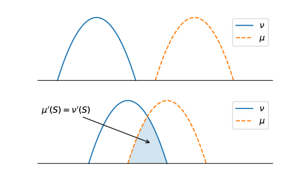
Figure 1. Densities and ordered component pairs

Axiom 4.1 adds the converse implication to (6), so $\delta$ identifies ordered pairs:

Proposition 4.1.

If $\delta$ is a measure of degree of stochastic dominance that satisfies Axiom 4.1, then $\delta(\mu,\nu)=1$ if and only if $\mu\preceq_{sd}\nu$.

Proof.

Suppose that $\delta$ satisfies Axiom 4.1 and that $\delta(\mu,\nu)=1$. Then $\mu^{\prime}(S)=\nu^{\prime}(S)=1$ for some $(\mu^{\prime},\nu^{\prime})$ in $\Phi(\mu,\nu)$. From this we immediately have $\mu^{\prime}=\mu$ and $\nu^{\prime}=\nu$, and hence $\mu\preceq_{sd}\nu$, which is all we need to show. ∎

The second axiom plays the opposite role. It implies that $\delta(\mu,\nu)$ is close to $1$ when $\mu$ is “nearly” dominated by $\nu$.

Axiom 4.2.

Given $\mu_{a},\mu_{b},\nu_{a},\nu_{b}\in\mathcal{P}$ and $\lambda\in[0,1]$, the ordering $\mu_{a}\preceq_{sd}\nu_{a}$ implies $\delta(\mu,\nu)\geq\lambda$ for $\mu:=\lambda\mu_{a}+(1-\lambda)\mu_{b}$ and $\nu:=\lambda\nu_{a}+(1-\lambda)\nu_{b}$.

Axiom 4.2 uses the natural convexity of $\mathcal{P}$ to implement “continuity near 1” while avoiding being tied to a particular topology.

The axioms we have listed are strong enough to give uniqueness:

Theorem 4.1.

The only measure of degree of stochastic dominance satisfying Axioms 4.1–4.2 is $\tau$.

Proof.

First we claim that $\tau$ satisfies Axiom 4.1. To see this, let $(X,Y)$ be an optimal coupling for $(\mu,\nu)$, attaining the maximum in (2). Set $\mu^{\prime}(B)=\mathbbm{P}\{X\in B,\,X\preceq Y\}$ and $\nu^{\prime}(B)=\mathbbm{P}\{Y\in B,\,X\preceq Y\}$. This pair satisfies $(\mu^{\prime},\nu^{\prime})\in\Phi(\mu,\nu)$ and $\mu^{\prime}(S)=\tau(\mu,\nu)$. To see that $\tau$ satisfies Axiom 4.2, fix $\mu,\nu\in\mathcal{P}$ and let the decompositions in Axiom 4.2 be given, with $\lambda\in[0,1]$ and $\mu_{a}\preceq_{sd}\nu_{a}$. Let $(X_{i},Y_{i})$ be an optimal coupling of $(\mu_{i},\nu_{i})$ for $i=a,b$. Let $X=\ell X_{a}+(1-\ell)X_{b}$ where $\ell$ is independent and binary with $\mathbbm{P}\{\ell=1\}=\lambda$. Let $Y=\ell Y_{a}+(1-\ell)Y_{b}$. Then $(X,Y)\in\Pi(\mu,\nu)$. Hence $\tau(\mu,\nu)\geq\mathbbm{P}\{X\preceq Y\}\geq\lambda\mathbbm{P}\{X_{a}\preceq Y_{a}\}=\lambda$, and Axiom 4.2 holds.

Now let $\delta$ be an arbitrary measure of degree of stochastic dominance satisfying Axioms 4.1–4.2. Fix $(\mu,\nu)$ in $\mathcal{P}\times\mathcal{P}$ and let $(X,Y)$ be an optimal coupling of $(\mu,\nu)$. Define $\lambda:=\mathbbm{P}\{X\preceq Y\}$ and the probabilities

$$\mu_{a}(B) =\frac{\mathbbm{P}\{X\in B,\;X\preceq Y\}}{\lambda},\quad\nu_{a}(B)=\frac{\mathbbm{P}\{Y\in B,\;X\preceq Y\}}{\lambda},$$

$$\mu_{b}(B) =\frac{\mathbbm{P}\{X\in B,\;X\npreceq Y\}}{1-\lambda},\quad\nu_{b}(B)=\frac{\mathbbm{P}\{Y\in B,\;X\npreceq Y\}}{1-\lambda}.$$

We have $\mu_{a}\preceq_{sd}\nu_{a}$, since, when $I\in\mathcal{B}$ is increasing,

$$\mu_{a}(I)=\frac{\mathbbm{P}\{X\in I,\;X\preceq Y\}}{\lambda}\leq\frac{\mathbbm{P}\{Y\in I,\;X\preceq Y\}}{\lambda}=\nu_{a}(I).$$

For $\mu$ we have $\mu(B)=\mathbbm{P}\{X\in B\}$, which can be decomposed as $\mathbbm{P}\{X\in B,\;X\preceq Y\}+\mathbbm{P}\{X\in B,\;X\npreceq Y\}=\lambda\mu_{a}(B)+(1-\lambda)\mu_{b}(B)$. Since $\delta$ satisfies Axiom 4.2, we have $\delta(\mu,\nu)\geq\lambda=\mathbbm{P}\{X\preceq Y\}=\tau(\mu,\nu)$.

For the reverse inequality, recall from the arguments above that we can obtain an ordered component pair $(\mu^{\prime},\nu^{\prime})$ satisfying $\nu^{\prime}(S)=\mu^{\prime}(S)=\tau(\mu,\nu)$. Since $\delta$ satisfies Axiom 4.1, we have $\delta(\mu,\nu)\leq\tau(\mu,\nu)+\epsilon$ for all $\epsilon>0$. Hence $\delta(\mu,\nu)\leq\tau(\mu,\nu)$. ∎

5. Measures vs Axioms

Let us reconsider measures of stochastic dominance other than $\tau$. By Theorem 4.1, they fail at least one of the axioms. For example, regarding Axiom 4.2, note that $q$ fails whenever the grid $\{x_{i}\}$ has at least three points. To see this let $F^{\prime}$, $F^{\prime\prime}$ and $G^{\prime\prime}$ be any cdfs on $[a,b]$ such that $F^{\prime\prime}<G^{\prime\prime}$ on $(a,b)$. Let $\lambda\in(0,1)$ and let

$$F=\lambda F^{\prime}+(1-\lambda)F^{\prime\prime},\quad G=\lambda F^{\prime}+(1-\lambda)G^{\prime\prime}.$$

Since $F^{\prime}\preceq_{sd}F^{\prime}$, Axiom 4.2 implies that $q(F,G)\geq\lambda$. On the other hand, $G(x_{i})>F(x_{i})$ on any interior point $x_{i}$. Hence $m$ in (7) is at most 2, and $q(F,G)\leq 2/n$. Since $\lambda$ can be arbitrarily close to 1 this contradicts Axiom 4.2.

For this same pair $F,G$, the fact that $G>F$ on $(a,b)$ implies that $c^{*}(F,G)=0$ for $c^{*}$ defined in (8), and hence $r(F,G)=0$ for the restricted stochastic dominance measure defined in (9). Likewise, for the same pair, $\alpha(F,G)=0$, where $\alpha$ is the almost stochastic dominance measure. Hence $r$ and $\alpha$ also fail to satisfy Axiom 4.2.

Regarding Axiom 4.1, the measures $q$, $r$ and $\alpha$ all fail. To see this, let $S=[0,1]$ and, given some positive number $\epsilon$, let $\mu$ put mass $\epsilon$ on $0$ and $1-\epsilon$ on $1$, and let $\nu$ put all mass on $1-\epsilon$. Let $F$ be the cdf of $\mu$ and let $X$ be a draw from $\mu$. Let $G$ and $Y$ be the cdf of and a draw from $\nu$ respectively. Since $Y$ is certainly $1-\epsilon$ we have $X\leq Y$ if and only if $X=0$, and hence $\mathbbm{P}\{X\leq Y\}=\epsilon$ for all couplings. On the other hand, $F(x)>G(x)$ iff $0\leq x<1-\epsilon$, and hence $r(F,G)=1-\epsilon$. If $\epsilon<1/2$ then $1-\epsilon>\epsilon$, and hence $r$ fails Axiom 4.1. The measures $q$ and $\alpha$ also give values larger than $\epsilon$ when $\epsilon$ is small, although the details are omitted.

6. Final Comments

We end with some avenues for future research. One is that an estimation theory for $\tau$ should be straightforward to construct. For example, if we replace the cdfs $F$ and $G$ in (5) with empirical counterparts $F_{n}$ and $G_{n}$, then $\tau(F_{n},G_{n})$ is a simple transform of the statistic used in the one-sided two-sample Kolmogorov-Smirnov test. This allows for construction of confidence intervals and hypotheses tests related to the value of $\tau$.

Another topic of interest is computation. In higher dimensional settings, computation is difficult for all measures of partial stochastic dominance, but $\tau$ at least has an interpretation as the solution to an optimal transport problem. Computing solutions of optimal transport problems is an active research area [10].

Third, there is some connection between the measure $\tau$, which takes values in the interval $[0,1]$ and represents the continuum between no dominance and complete first order dominance, and the measure proposed in [9], which represents the continuum between first order and second order stochastic dominance. Clarifying this connection and investigating the preceding two topics are left for future work.

7. Acknowledgements

We gratefully acknowledge JSPS KAKENHI Grant 15H05729 and Australian Research Council Grant DP120100321.

References

- [1] Anthony B Atkinson. On the measurement of poverty. Econometrica, 55(4):749–764, 1987.
- [2] Russell Davidson and Jean-Yves Duclos. Statistical inference for stochastic dominance and for the measurement of poverty and inequality. Econometrica, 68(6):1435–1464, 2000.
- [3] Russell Davidson and Jean-Yves Duclos. Testing for restricted stochastic dominance. Econometric Reviews, 32(1):84–125, 2013.
- [4] Gary S Fields, Jesse B Leary, and Efe A Ok. Stochastic dominance in mobility analysis. Economics Letters, 75(3):333–339, 2002.
- [5] Hans Föllmer and Alexander Schied. Stochastic Finance: An Introduction in Discrete Time. De Gruyter Textbook Series. De Gruyter, 2011.
- [6] Moshe Leshno and Haim Levy. Preferred by “all” and preferred by “most” decision makers: Almost stochastic dominance. Management Science, 48(8):1074–1085, 2002.
- [7] Haim Levy. Stochastic dominance and expected utility: survey and analysis. Management Science, 38(4):555–593, 1992.
- [8] Moshe Levy. Almost stochastic dominance and stocks for the long run. European Journal of Operational Research, 194(1):250–257, 2009.
- [9] Alfred Müller, Marco Scarsini, Ilia Tsetlin, and Robert L Winkler. Between first-and second-order stochastic dominance. Management Science, 63(9):2933–2947, 2017.
- [10] Gabriel Peyré and Marco Cuturi. Computational optimal transport. Now Publishers, 2019.
- [11] Stoyan V Stoyanov, Svetlozar T Rachev, and Frank J Fabozzi. Metrization of stochastic dominance rules. International Journal of Theoretical and Applied Finance, 15(02), 2012.
- [12] Volker Strassen. The existence of probability measures with given marginals. The Annals of Mathematical Statistics, pages 423–439, 1965.
- [13] Cédric Villani. Optimal transport: old and new. Springer Science, 2008.