geom2vec: pretrained GNNs as geometric featurizers for conformational dynamics

Abstract

Identifying informative low-dimensional features that characterize dynamics in molecular simulations remains a challenge, often requiring extensive hand-tuning and system-specific knowledge. Here, we introduce geom2vec, in which pretrained graph neural networks (GNNs) are used as universal geometric featurizers. By pretraining equivariant GNNs on a large dataset of molecular conformations with a self-supervised denoising objective, we learn transferable structural representations that capture molecular geometric patterns without further fine-tuning. We show that the learned representations can be directly used to analyze trajectory data, thus eliminating the need for manual feature selection and improving robustness of the simulation analysis workflows. Importantly, by decoupling GNN training from training for downstream tasks, we enable analysis of larger molecular graphs with limited computational resources.

I Introduction

Molecular dynamics simulations can provide atomistic insight into complex reaction dynamics, but their high dimensionality makes them hard to interpret. Analyses thus rely on identifying low-dimensional representations (features), and care is needed in choosing them because they can strongly impact conclusions [1, 2, 3, 4]. Often features are selected manually, but doing so relies on system-specific intuition. Because developing intuition is often the goal of simulations, many researchers instead turn to machine-learning methods for constructing features that capture observed variance (e.g., principal component analysis) [5, 6, 7] or decorrelate slowly according to the simulation data (e.g., following the variational approach for Markov processes, VAMP) [8, 9, 10, 11]. While these objectives are not always aligned with the reaction of interest [12, 13, 3, 4], such features can serve as useful intermediaries for computing reaction-specific statistics [14, 13] that provide a principled way for evaluating mechanisms [15, 16].

Generally the inputs to the machine-learning methods above are internal coordinates such as distances between selected atoms and dihedral angles because they are invariant to translations and rotations of the system. However, the nonlocal nature of these coordinates and/or their effects (e.g., the rotation of a dihedral angle in a polymer backbone) can make the resulting features both ineffective and hard to interpret, and these issues become more significant with system size. Additionally, it is not obvious how to represent permutationally invariant species such as solvent molecules with internal coordinates; recently introduced machine learning approaches for treating such species do not scale well with system size [17].

Because atoms and their interactions (through bond or through space) can be viewed as the nodes and edges of graphs, molecular information can be readily encoded in graph representations (e.g., graph neural networks, GNNs). Importantly, graph representations can be constructed in ways that respect the symmetries of molecular systems, with translational, rotational, and permutational invariance and equivariance. Equivariance allows, for example, GNNs to output forces that rotate with the system, and appears to improve learning [18, 19, 20]. Owing to both their conceptual appeal and their performance, GNNs now dominate machine learning for force fields and molecular property prediction [21, 20, 22, 23, 24]. They also are being successfully used to learn representations of larger molecules for tasks such as protein structure prediction, design, fold classification, and function prediction [25, 26, 27, 28, 29].

The tasks above concern prediction of static properties, including structures. Because molecular dynamics trajectories consist of sequences of structures, GNNs should be useful for identifying features for computing reaction statistics, and several groups have married GNNs with VAMP [8] to learn metastable states and relaxation time scales of both materials and biomolecules [30, 31, 32, 33, 34]. These groups report improved variational scores, convergence for shorter lag times, and more interpretable learned representations relative to VAMPnets based on fully connected networks. However, the graphs in these studies are small, either because the molecules are small, or only a subset of atoms (e.g., the C_α atoms of proteins) are used as inputs. As we discuss below, existing GNNs for analyzing dynamics do not readily scale to larger numbers of atoms nor transfer across molecular systems, which limits their ability to go beyond approaches based on manually chosen features.

The key idea of this paper is that GNNs can be pretrained using independent structural data prior to their use to analyze dynamics, thus decoupling GNN training from training for downstream tasks. Pretraining has transformed other domains such as natural language processing (NLP) and computer vision. In these cases, pretraining enables high-dimensional latent representations of words (“tokens”) [35] or images (“patches”) [36] to be learned by self-supervised, auto-regressive training. In NLP, word2vec pioneered the idea of using learnable vector representations for words, assigning them based on the word itself and its surrounding context [37]; these representations could then be used for diverse downstream tasks. Inspired by word2vec, we propose geom2vec, an approach that leverages pretrained GNNs to learn transferable vector representations for molecular geometries.

Various pretraining strategies have been tried in molecular contexts [38, 39, 26, 40, 28, 25], but in contrast to complex pretraining and encoding schemes devised for specific classes of molecules [28, 25], we use a scheme that can be applied generally. Building on the idea that corrupting data with noise and training a model to reconstruct the original data (denoising) can lead to learning meaningful representations for generative models [41, 42], Zaidi et al. [40] showed that denoising atomic coordinates of structures of organic molecules significantly improved GNN performance on a number of molecular property prediction benchmarks.

Here, we show that this simple pretraining scheme also accelerates analysis of molecular dynamics simulations. Specifically, we pretrain GNNs using the same denoising objective and a dataset of organic molecules optimized with density functional theory [43] and analyze protein molecular dynamics simulations with the resulting representations. We consider two tasks: learning slowly decorrelating modes with VAMP [8] and identifying metastable states with the state predictive information bottleneck (SPIB) framework [44, 45]. We show that neural networks trained using the GNN representations can readily take all atoms in a small protein as inputs, enabling, for example, discovery of side chain dynamics that are important for folding. By decoupling learning molecular representations from training for specific tasks, our method naturally accommodates alternative pretraining schemes [25, 28] and datasets [46] (e.g., ones specific to particular classes of molecules), as well as other possible tasks [47, 48, 49, 50, 51].

II Methods

The basic idea of our method is to pretrain a GNN using a suitable task (here, denoising molecular coordinates) and then to use it with the resulting parameter values fixed as a feature encoder for other (downstream) tasks, as summarized in Figure 1. In this section, we provide an overview of the network architecture that we use and then describe its elaboration for the pretraining and downstream tasks; further details are provided in the Supporting Information. We refer to the workflow of transforming the atomic coordinates to embedding vectors (i.e., features) and the use of those vectors as “geom2vec.”

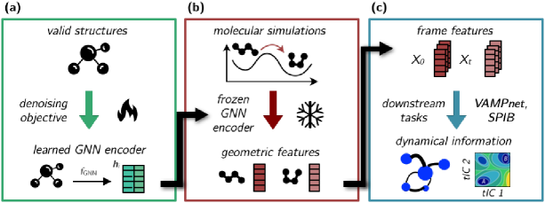
Figure 1: The geom2vec workflow. (a) A GNN encoder is pretrained using a denoising objective on a dataset of structures of diverse molecules. (b) Geometric representations for configurations from molecular simulations are obtained by performing inference with the pretrained GNN encoder. (c) The representations are used as inputs to a downstream task head (here, a VAMPnet or SPIB), which is trained separately.

II.1 Network architecture

As noted above, our goal is learn a mapping from Cartesian coordinates to embedding vectors via a GNN. There are many existing GNN architectures from which to choose [24]. Here, we use the ViSNet [52] architecture, which is built on TorchMD-ET[53]. These are both equivariant geometric graph transformers with modified attention mechanisms that suppress interactions between distant atoms; ViSNet goes beyond TorchMD-ET in using (standard and improper) dihedral angle information in its internal representations. Both architectures output three-dimensional vector features, which change appropriately with molecular translation and rotation, as well as one-dimensional scalar features, which are invariant to molecular translation and rotation. That is,

$$f_{\text{GNN}}:\mathbb{R}^{3N}\rightarrow\mathbb{R}^{(1+3)dN},$$ (1)

where $N$ is the number of atoms, and $d$ is the number of features associated with each atom (equal to the dimension of the last update layer). We represent the features for atom $i$ by $\mathbf{h}_{i}\in\mathbb{R}^{(1+3)d}$. We choose ViSNet because it was previously shown to give accurate molecular property predictions and accurate conformational distributions when used to learn a potential for molecular dynamics simulations. [52] We briefly introduce the TorchMD-ET and ViSNet architectures in Appendices A.2 and A.3, and we refer interested readers to the original publications for further details.

II.2 Pretraining by denoising

For the pretraining, we draw random displacements from a multivariate Gaussian distribution and add them to the Cartesian coordinates of the molecules in the training set; we then train the GNN to predict the displacements. This process is designed to encourage the network to learn representations that capture the geometry of the molecular conformations, and it can be viewed as learning a force field with energy minima close to the training set geometries [40]. We choose this objective because structural data are more readily available than energetic data, especially for large molecules such as proteins.

Here, we use the OrbNet Denali dataset, which consists of 215,000 molecules and complexes (with an average of 45 atoms) with 2.3 million conformations sampled from molecular trajectories [43]. We randomly select 10,000 conformations for validation and use the remainder for training.

Following Zaidi et al. [40], we pretrain the model by passing the $(1+3)d$ features for each atom (graph node) from the ViSNet architecture through a gated equivariant block (Algorithm 1) that combines the $d$ scalar and vector features to obtain a three-dimensional vector that represents the predictions for the displacement of that atom. We train for a fixed number of epochs and save the parameters resulting in the lowest mean squared error (MSE) between the predicted and normalized added atom displacements with a unit variance for the validation set. Further details, including hyperparameters, are given in Appendix D. Depending on the network architecture, configuration and graphics card available, the one-time pre-training can take from several hours to a few days.

II.3 Use of the representations

In this section, we discuss the operational details of using the pretrained GNN for downstream tasks in general (summarized in Figure 1). The specific downstream tasks that we use for our numerical demonstrations are described in Section III.

II.3.1 Atom selection

We first select the atoms of interest. For example, when analyzing simulations with explicit solvent, we may select only the solute coordinates. Given the molecular coordinates, the pretrained GNN yields a learned representation $\mathbf{h}_{i}$ for each selected atom $i$. One can choose to base the calculations for the downstream tasks on the atomic embedding vectors and/or the sums over their $d$ scalar and vector elements, but in most cases we reduce the size of the graph by coarse-graining the system, as we now describe.

II.3.2 Coarse-graining

Let $\mathcal{S}=\{S_{1},\dots,S_{M}\}$ be a partition of the atoms into $M$ disjoint subsets, where each subset $S_{m}$ contains atoms belonging to a structural unit, such as a functional group or monomer in a polymer, depending on the system. We pool the atomic representations for each $S_{m}$:

$$\bar{\mathbf{h}}_{S_{m}}=\sum_{i\in S_{m}}\mathbf{h}_{i}.$$ (2)

Each resulting coarse-grained embedding vector $\bar{\mathbf{h}}_{S_{m}}$ represents the geometric information of the atoms within its structural unit in an average sense. Following the NLP literature, we refer to the coarse-grained representations as structural “tokens.” The advantage of coarse-graining is that it typically reduces the number of nodes in the graph by an order of magnitude.

II.3.3 Feature combination

To use the coarse-grained tokens in a learning task, we must combine their information in a useful fashion. How best to do so depends on the structural properties of interest, but we can generally lump approaches into two categories:

• Pooling: We sum (or average) the coarse-grained tokens to obtain a single, global representation of the molecular system $\bar{\mathbf{h}}\in\mathbb{R}^{(1+3)d}$. Note that this approach is equivalent to pooling the atomic embedding vectors $\mathbf{h}_{i}$.

• Token mixing: This approach applies a learnable mixing operation to the coarse-grained tokens to capture their interactions and dependencies [54]. In this work, we employ three kinds of token mixers: (1) a standard transformer architecture [35], which we refer to as “SubFormer;” (2) an MLP-mixer architecture[55], which we refer to as “SubMixer;”[56] (3) the geometric vector perceptron (GVP) architecture, an equivariant GNN introduced for biomolecular modeling [57]. SubFormer and SubMixer can be combined with GVP and/or augmented with a special token that encodes global information [58] such as pairwise distances (see Algorithms 2 and 3 in Appendix B).

Pooling has the advantage that it does not require training. On the other hand, token mixers allow for greater expressivity and can capture complex interactions between structural units.

II.4 Output layers

Ultimately, we combine the features from the different graph nodes and any graph-wide information (e.g., the CLS token of the transformer) and use an MLP to output quantities specific to a downstream task. Here, we consider downstream tasks that require only scalar quantities, so we input only the scalar features to the MLP, but generally scalar (invariant) and vector (equivariant) quantities can be input and output. We summarize the overall scheme in Algorithm 3.

III Downstream tasks

To assess whether the geom2vec representations are useful for learning protein dynamics, we apply them to learning slowly decorrelating modes with VAMP [8] and identifying metastable states with the state predictive information bottleneck (SPIB) framework [44]. As described previously, we apply the pretrained GNN to the coordinates from molecular dynamics trajectories and then use the resulting features as inputs to the desired task without further fine-tuning the GNN parameters. In this section, we briefly describe the two downstream tasks mathematically.

III.1 VAMPnets

Let $\mathbf{X}_{t}$ be a Markov process and define the correlation functions

$$C_{00} =\operatorname{\mathbf{E}}_{\mathbf{X}_{0}\sim\mu}[\chi_{0}(\tilde{\mathbf{h}}(\mathbf{X}_{0}))\chi_{0}^{\mathsf{T}}(\tilde{\mathbf{h}}(\mathbf{X}_{0}))]$$ (3)

$$C_{01} =\operatorname{\mathbf{E}}_{\mathbf{X}_{0}\sim\mu}[\chi_{0}(\tilde{\mathbf{h}}(\mathbf{X}_{0}))\chi_{1}^{\mathsf{T}}(\tilde{\mathbf{h}}(\mathbf{X}_{\tau}))]$$ (4)

$$C_{11} =\operatorname{\mathbf{E}}_{\mathbf{X}_{0}\sim\mu}[\chi_{1}(\tilde{\mathbf{h}}(\mathbf{X}_{\tau}))\chi_{1}^{\mathsf{T}}(\tilde{\mathbf{h}}(\mathbf{X}_{\tau}))],$$ (5)

where $\chi_{0}$ and $\chi_{1}$ are vectors of functions and the expectation is over trajectories initialized from an arbitrary distribution $\mu$. In our case, $\mathbf{X}_{t}$ represents the molecular coordinates at time $t$, $\chi_{0}$ and $\chi_{1}$ represent vectors of features, and $\tilde{\mathbf{h}}(\mathbf{X})$ is the output of a geom2vec block. In the limit that $\chi_{0}$ and $\chi_{1}$ are infinite-dimensional, the dynamics can be encoded through the action of a linear transformation[8, 59]:

$$\operatorname{\mathbf{E}}[\chi_{1}(\tilde{\mathbf{h}}(\mathbf{X}_{\tau}))]=T^{\mathsf{T}}\operatorname{\mathbf{E}}[\chi_{0}(\tilde{\mathbf{h}}(\mathbf{X}_{0}))].$$ (6)

For finite-dimensional $\chi_{0}$ and $\chi_{1}$, the relation is approximate. The variational approach for Markov processes (VAMP)[9, 60, 8, 61] represents $\chi_{0}$ and $\chi_{1}$ by the dominant $k$ left and right singular vectors of $T$, respectively. In this case, $T=C_{00}^{-1}C_{01}$ satisfies (6) in a least-squares sense (i.e., minimizes $\operatorname{\mathbf{E}}[\|\chi_{1}(\tilde{\mathbf{h}}(\mathbf{X}_{\tau}))-T^{\mathsf{T}}\chi_{0}(\tilde{\mathbf{h}}(\mathbf{X}_{0}))\|^{2}]$) and $\chi_{0}$ and $\chi_{1}$ maximize the VAMP-2 score:

$$\text{VAMP-2}=\left\lVert C_{00}^{-1/2}C_{01}C_{11}^{-1/2}\right\rVert_{F}^{2},$$ (7)

where the subscript $F$ denotes the Frobenius norm.

Operationally, the components of $\chi_{0}$ and $\chi_{1}$ are learned from data by representing them by parameterized functions (e.g., neural networks in VAMPnets [8]) and maximizing (7). VAMPnets require one to specify the output dimension ($k$ above) a priori. For the benchmark systems that we consider, we choose $k$ based on previous results in the literature.

As discussed below (Section IV.4) we split each dataset into training and validation sets, evaluating the validation score every 10 training steps. Each training step or validation step, we randomly draw a batch of trajectory-frame pairs spaced by $\tau$ to compute (7). Because the loss function (7) requires estimating correlation matrices and their inverses, we found that a large batch size (at least 5000 for the examples here) was required to minimize the variance during training. To prevent overfitting, we apply an early stopping criterion[11]: we stop training when the training VAMP score does not increase for 1000 batches or the validation VAMP score does not increase for 10 batches. Further training details are given in Table S2.

III.2 State Predictive Information Bottleneck (SPIB)

In the information bottleneck (IB) framework, an encoder-decoder setup is used to learn a low-dimensional (latent) representation $\mathbf{z}$ that minimizes the information from a high-dimensional input $\mathbf{x}$ while maximizing the information about a target $\mathbf{y}$. The associated loss function is

$$\mathcal{L}_{\mathrm{IB}}=I(\mathbf{z},\mathbf{y})-\beta I(\mathbf{x},\mathbf{z}),$$ (8)

where $I$ refers to the mutual information between two random variables:

$$I(A,B)=\int\int p(A,B)\ln\frac{p(A,B)}{p(A)p(B)}\,dA\,dB,$$ (9)

and the parameter $\beta$ controls the tradeoff between prediction accuracy and the complexity of the latent representation.

In the state predictive information bottleneck (SPIB) extension of IB [62], the inputs are parameterized molecular features at time $t$, $\tilde{\mathbf{h}}(\mathbf{X}_{t})$, and the targets are one-hot vectors $y^{s}_{t}$ that indicate the state of the system (i.e., $y^{s}_{t}=1$ when the system is in state $s$ at time $t$). The latent representation and state indicators are learned simultaneously by predicting the state indicators at time $t+\tau$ given the molecular features at time $t$.

To learn the latent representation $z$, SPIB maximizes the loss function

$$\mathcal{L}_{\text{SPIB}}=\operatorname{\mathbf{E}}_{\mathbf{X}_{0}\sim\mu,\mathbf{z}\sim p_{\theta}(\mathbf{z}|\tilde{\mathbf{h}}(\mathbf{X}_{0}))}\Biggl{[}\ln q_{\theta}(\mathbf{y}_{\tau}|\mathbf{z})\\ -\beta\ln\frac{p_{\theta}(\mathbf{z}|\tilde{\mathbf{h}}(\mathbf{X}_{0}))}{r_{\theta}(\mathbf{z})}\Biggr{]}.$$ (10)

The encoder generates the latent representation $z$ from the input with probability $p_{\theta}(\mathbf{z}|\tilde{\mathbf{h}}(\mathbf{X}))=\mathcal{N}(z;\mu_{\theta}(\tilde{\mathbf{h}}(\mathbf{X})),\Sigma_{\theta}(\tilde{\mathbf{h}}(\mathbf{X})))$, which is a multivariate normal distribution with learned mean $\mu_{\theta}(\tilde{\mathbf{h}}(\mathbf{X}))$ and learned covariance $\Sigma_{\theta}(\tilde{\mathbf{h}}(\mathbf{X}))$. The decoder takes the latent representation $\mathbf{z}$ and returns the probability $q_{\theta}(y^{s}|\mathbf{z})$ of each state indicator $y^{s}$; $q_{\theta}(y^{s}|\mathbf{z})$ is represented by a neural network with output dimension $k$. The quantity $r_{\theta}(\mathbf{z})$ is a prior. The state indicators are updated during training as follows:

$$y_{\tau}^{s}=\begin{cases}1&\text{if }s=\operatorname{arg\,max}_{y}q_{\theta}(y|\mu_{\theta}(\tilde{\mathbf{h}}(\mathbf{X}_{\tau}))),\\ 0&\text{otherwise}.\end{cases}$$ (11)

We follow Wang and Tiwary [44] and use a variational mixture of posteriors for the prior [63]:

$$r_{\theta}(\mathbf{z})=\left.\sum_{i}\omega_{i}p_{\theta}(\mathbf{z}|u_{i})\right/\sum_{i}\omega_{i},$$ (12)

where $\omega$ and $u$ are learned parameters. In this work, we prepared the initial state labels by performing k-means clustering on the collective variables (CVs) learned from VAMPnets based on distances between C_α atoms with $k=100$ clusters. Further training details are given in Table S3.

IV Systems studied

We examine the performance of geom2vec for analyzing data from long molecular dynamics simulations of three well-characterized fast-folding proteins (chignolin, trp-cage, and villin) [64]. The data for each system is a single, unbiased simulation, which we assume approximately samples the equilibrium distribution. In this section, we introduce each system and briefly describe its structure and dynamics.

IV.1 Chignolin

Chignolin is a 10-residue fast-folding protein with sequence YYDPETGTWY. The folded state consists of three $\beta$-hairpin structures that are distinguished by hydrogen bonding between the threonine side chains and their dihedral angles, which interconvert on the nanosecond timescale [50]. The trajectory that we analyze is 106 $\mu$s long at 340 K and saved every 0.2 ns [64]. For VAMPnet fitting, we choose $k=3$.

IV.2 Trp-cage

Trp-cage is a 20-residue fast-folding protein; here we study the K8A mutant with sequence DAYAQWLADGGPSSGRPPPS. Its secondary structure consists of an $\alpha$-helix (residues 2–9), a short $3_{10}$-helix (residues 11–14), and a polyproline II helix (residues 17–19); the protein takes its name from Trp6, which is in the core of the folded state. The trajectory is 208 $\mu$s long at 290 K and saved every 0.2 ns. Previous studies of this trajectory generally identified the folded and unfolded states, with varying numbers of intermediates and misfolded states [65, 45]. For VAMPnet fitting, we choose $k=4$.

IV.3 Villin

The 35-residue villin headpiece subdomain (HP35) [66] is a fast-folding protein with sequence LSDEDFKAVFGMTRSAFANLPLWnLQQHLnLKEKGLF where nL refers to the unnatural amino acid norleucine. The K65nL/N68H/K70nL mutant was engineered to fold more rapidly [67]. The secondary structure of villin consists of three $\alpha$-helices at residues 3–10, 14–19, and 22–32. Villin has a hydrophobic core centered on residues Phe6, Phe10, and Phe17. The trajectory that we study is 125 $\mu$s long at 360 K and saved every 0.2 ns [64]. Previous studies typically identified three states: a folded state, an unfolded state, and a misfolded state [11]. Wang et al. [68] proposed two primary folding pathways, where either the C-terminus or the N-terminus folds first, ultimately leading to the native state. Additionally, a cooperative hydrophobic interaction may facilitate a third folding pathway. For VAMPnet fitting, we choose $k=3$.

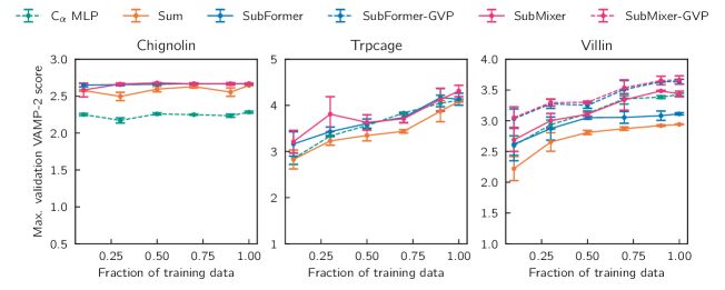
Figure 2: VAMPnets with varying geom2vec architectures. The amount of training data was varied by dividing the training data into 20 trajectory segments of equal length and then randomly selecting the indicated fraction for training. The validation set is held fixed as the second half of each trajectory. Error bars show standard errors over three independent runs.

IV.4 Training-validation split

Although previous studies used a random split[8, 32, 69], we observe that, due to the strong correlation between successive structures sampled by molecular dynamics simulations, a random split allows networks to achieve high validation scores even when they have memorized the training data rather than learned useful abstractions from it; the models then perform poorly on independent data. Consequently, for all our numerical experiments, we split the data into training and validation sets by time. That is, we select the first 50% of the long trajectory for training and the remainder for validation. If we had access to multiple independent trajectories, randomly choosing trajectories for training and validation would also be appropriate. Some studies split the trajectory into equal segments and draw random segments for training and validation [65, 45] (k-fold cross validation). When there are only two segments, this approach is identical to ours. When every structure is its own segment, one recovers the random split. Intermediate numbers of segments result in intermediate amounts of correlation between the training and validation sets. In cases where we vary the amount of training data, we first split the trajectory and then divide only the training dataset into segments that we draw randomly; this is fundamentally different from the approach in Refs. 45 and 65 and minimizes the correlation between the training and validation datasets.

V Results

V.1 VAMPNets

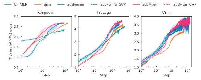
Figure S1: Training curves for VAMPnets on all three systems and all three mixers studied. Each curve represents the mean of three training runs. Shaded regions indicate standard error over three runs.

For each system and mixer architecture pair that we consider, we independently train three VAMPnets using different random number generator seeds (and the training-validation split described in Section IV.4). We report the training and validation VAMP-2 scores for the different mixer architectures for each of the three systems in Figures S1 and S2. For chignolin, GNNs with pooling (summing), SubMixer, and SubFormer reach approximately the same maximum validation score. GNNs with SubMixer and SubFormer require fewer epochs to reach the convergence criteria, but they require more computational time per epoch, as we discuss in Section VI. For both villin and trp-cage, the mixers generally outperform pooling.

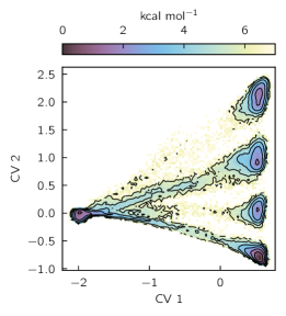
Figure 3: Potential of mean force (PMF) of chignolin as a function of the first two CVs learned by a VAMPnet trained with SubMixer. Contours are drawn every 1 kcal/mol. See Figure S3, S4, and S5 for corresponding plots for other architectures and proteins.

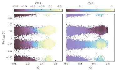
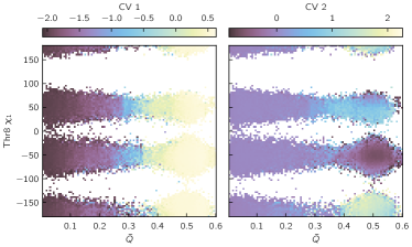
Figure 4: Chignolin VAMPnet (with SubMixer) CVs as a function of two physical coordinates: the fraction of native contacts and the $\chi_{1}$ side chain dihedral angle of Thr6 (left) and Thr8 (right). $\bar{Q}$ is the fraction of native contacts smoothed with a 1-ns moving window. We define native contacts as two residues that are at least three positions apart in sequence and have at least one distance between non-hydrogen atoms that is less than 4.5 Å in the crystal structure (5AWL[70]). See Figures S6 and S7 for analogous plots for trp-cage and villin.

Figure 2 displays the learning curves for VAMPNets with different training data sizes, varying from 5% to 50% of the available data. For chignolin, the GNNs clearly outperform a multilayer perceptron (MLP) that takes distances between pairs of C_α atoms as inputs; there is not a significant difference between pooling and the mixers considered. For trp-cage and villin, the GNN with pooling consistently achieves the lowest scores. The distance-based MLP and GNN with Submixer perform comparably, presumably because the distances between pairs of C_α atoms are sufficient to describe the folding (in contrast to chignolin, as we discuss below). For villin, we combined SubMixer and SubFormer with GVP and augmented them with a global token; this enables the GNNs to outperform the distance-based MLP. The improvement is particularly striking for SubFormer. The models with GVP are more expressive because they use the equivariant features at the token mixing stage and directly mix with global features after message-passing. We note that the VAMP scores that we achieve are lower than published ones owing to our choice of the training-validation split (Section IV.4) and output dimension $k$. While the amount of data does not significantly impact the performance for chignolin, the trp-cage and villin results suggest that additional data would permit achieving higher scores.

To visualize the results, we build histograms of learned CV-value pairs, which we convert to potentials of mean force (PMFs) by taking the logarithm and multiplying by the inverse temperature (Figures 3, S3, S4, and S5). We also show average values of CVs as functions of physically-motivated coordinates (Figure 4, S6, and S7).

The advantages of the GNN architecture are well illustrated by the results for chignolin. Previous machine-learning studies of chignolin identified two slow CVs, one for the folding-unfolding transition and one distinguishing competing folded states[50, 71]. Our VAMPnets appear to recover these two CVs (Figures 3 and S3; results shown are with SubMixer), distinguishing folded and unfolded states with CV 1 and four folded states with CV 2. To understand the physical differences between the folded states, we plot CVs 1 and 2 as functions of the fraction of native contacts and the $\chi_{1}$ side chain dihedral of Thr6 or Thr8 (Figure 4). The fraction of native contacts clearly correlates with CV 1, consistent with earlier studies. CV 2 distinguishes the folded states by the configurations of Thr6 and Thr8 side chains, which can each occupy two rotamers, yielding four possible folded states. These side chain dynamics could not be detected by VAMPnets that take backbone internal coordinates as inputs, as is common, or even GNNs limited to backbone atoms (the authors of Ref. 50 included distances to side chain atoms and then manually curated the inputs). This makes clear the usefulness of the pre-training approach that we take here, which enables treating all the atoms with an architecture that supports both scalar and vector features.

V.2 SPIB

V.2.1 Trp-cage

Figure 5 shows a Markov state model based on the states learned for trp-cage with a lag time of 20 ns. There are 13 long-lived states. State $S_{11}$ represents the folded ensemble with a well-defined structure. In states $S_{1}$ and $S_{2}$ the $\alpha$-helix is folded, and the $3_{10}$-helix and polyproline II helix are unfolded. In contrast, in state $S_{8}$ the $3_{10}$-helix is folded, and the $\alpha$-helix and polyproline II helix are unfolded. State $S_{5}$ represents a fully unfolded state, which acts as a hub that connects all intermediate states and the folded state, $S_{11}$. States $S_{3}$, $S_{4}$, $S_{6}$, $S_{7}$, $S_{9}$, $S_{10}$, and $S_{12}$ are also largely unfolded and differ with regard to the specific conformations of the helices.

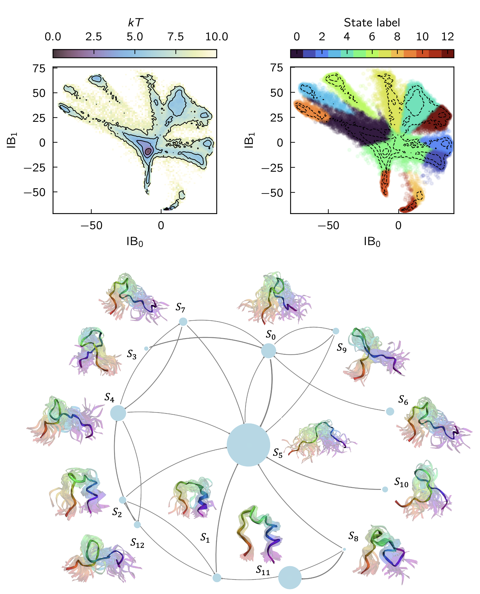
Figure 5: SPIB for trp-cage. All results are obtained from a GNN with SubFormer-GVP mixer. (top left) PMF as a function of the first two information bottleneck coordinates (IBs). Contours are drawn every 2 $kT$. (top right) Same contours colored by SPIB assigned labels. (bottom) Learned Markov State Model. The highlighted structures are chosen randomly from the trajectory. The N-terminus is violet and the C-terminus is red.

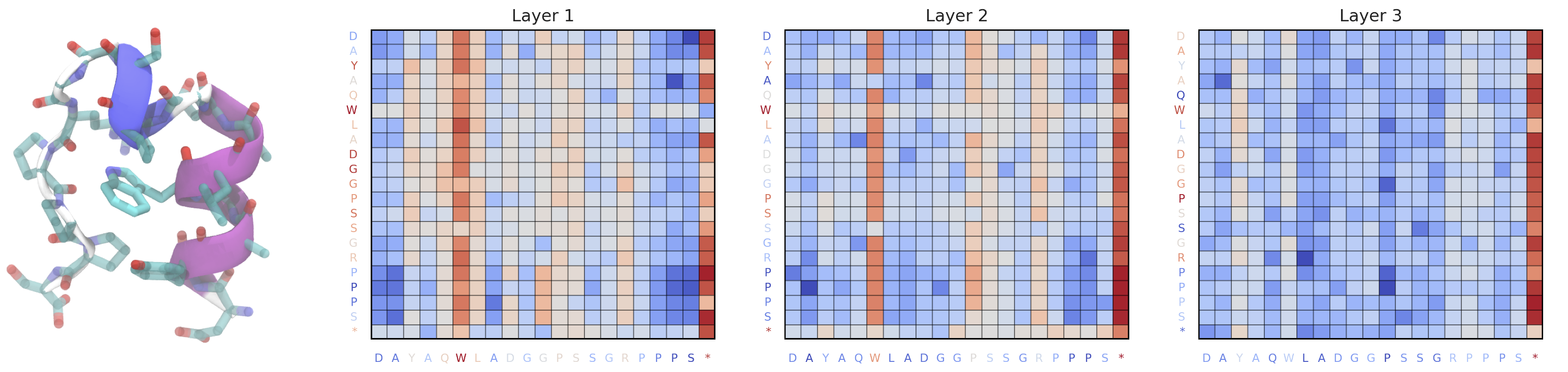
Figure 6: SPIB SubFormer-GVP attention. (left) A typical fully folded (classified as $S_{1}1$) trp-cage structure with the central tryptophan residue (Trp6/W6) highlighted. (right three plots) Log-scaled averaged attention maps from three layers of the Subformer block in the Subformer-GVP architecture. The sequence is indicated by one-letter amino acid codes, and $*$ represents a global token that encodes pairwise distances between the C_α atoms. Tokens from query and key projections are colored according to the row-wise and column-wise sum of layer-wise attention weights. Results shown are for all structures from the trajectory. Results for individual states are in Figures S8, S9, and S10.

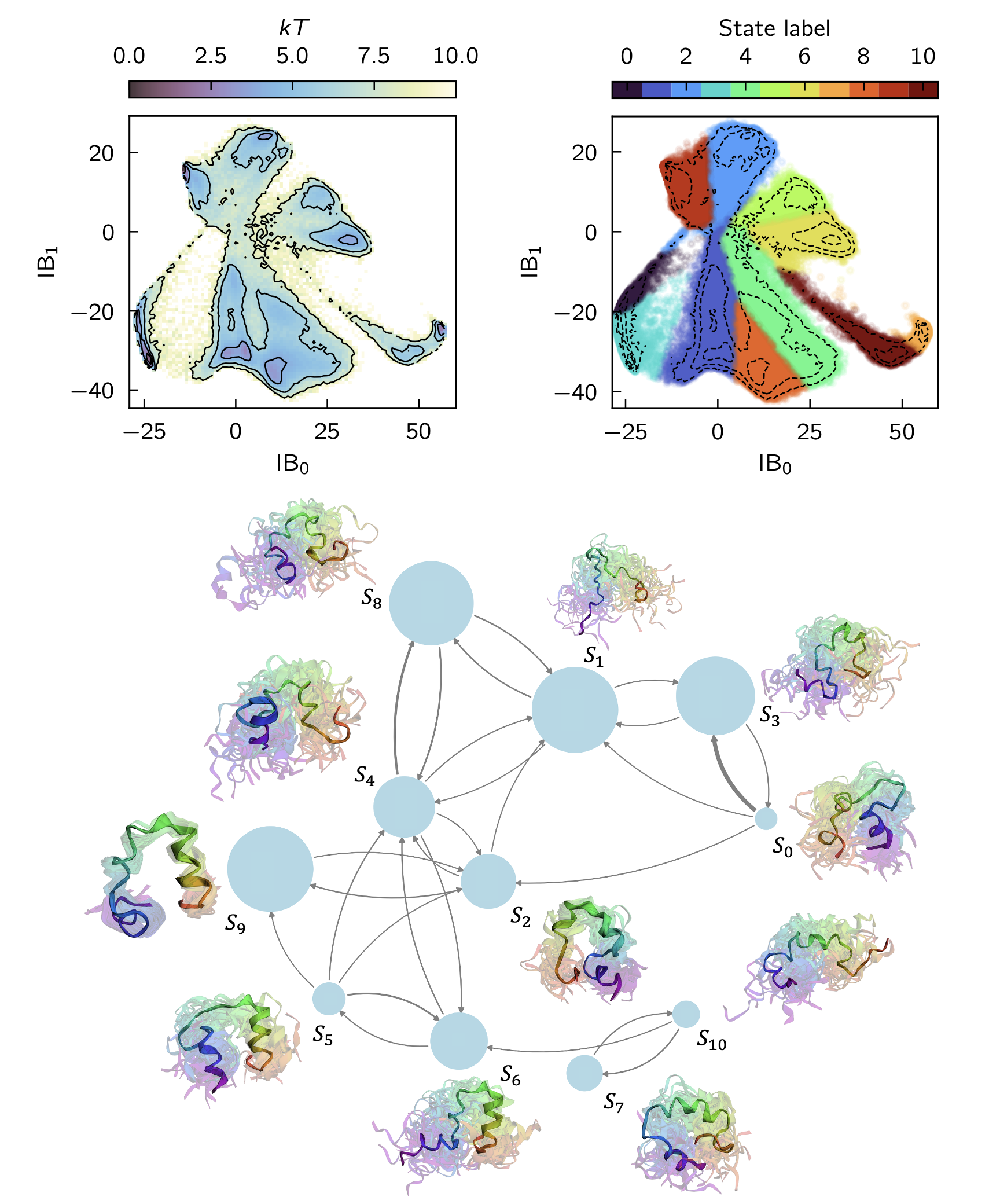
Figure 7: SPIB for villin. All results are obtained from a GNN with SubFormer-GVP mixer. (top left) PMF as a function of the first two information bottleneck coordinates (IBs). Contours are drawn every 1 $kT$. (top right) Same contours colored by SPIB assigned labels. (bottom) Learned Markov State Model. The highlighted structures are chosen randomly from the trajectory. The N-terminus is violet and the C-terminus is red.

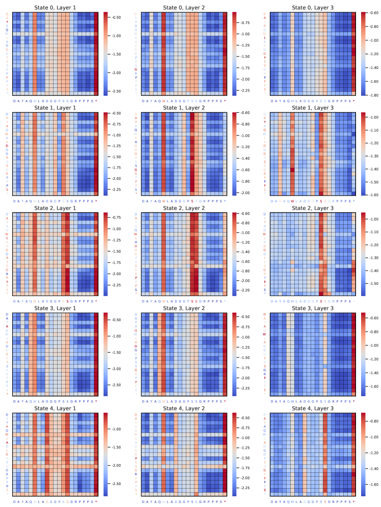
Figure S8: Log-scaled attention weight heatmaps for trp-cage SPIB states 0 to 4 from three layers of Subformer-GVP. Each subplot displays attention weights with color-coded tick labels based on normalized sums. Colorbars indicate log-scaled attention values.

We show attention maps of the SubFormer blocks averaged over all structures in Figure 6 and over the structures in each state in Figures S8, S9, and S10. The attention maps are $(N+1)\times(N+1)$ matrices, where for trp-cage $N=20$ represents the sequence positions, and the additional row and column correspond to a global token that encodes pairwise distances between the C_α atoms [56, 58]. The learned attention maps can be interpreted in terms of the structure. The residues that are most consistently activated across states and layers are Trp6 (W6) and Asp9-Ser14 (D9-S14), which roughly correspond to the 3₁₀-helix. Tyr3 (Y3), Gln5 (Q5), Gly15 (G15), and Arg16 (R16) are activated in selected states. The attention thus appears to track the packing of residues around Trp6. Across all three layers, the global token remains highly active, consistent with the fact that the long-lived states of trp-cage are reasonably well-characterized by the distances between the C_α atoms [65, 13]. The fact that tokens other than the global token participate in the attention mechanism again underscores the ability of GNNs to go beyond distances between C_α atoms.

V.2.2 Villin

Figure 7 shows a Markov state model based on the states learned for villin HP35 with a lag time of 10 ns. There are 11 long-lived states. State $S_{9}$ represents the fully folded structure, in which all three $\alpha$-helices are folded and packed compactly. States $S_{1}$ and $S_{3}$ correspond to fully unfolded states. In states $S_{0}$ and $S_{2}$ helix 1 is folded, suggesting a pathway in which folding initiates at the N-terminus, while in states $S_{5}$ and $S_{6}$ helix 3 is folded, suggesting a pathway in which folding initiates at the C-terminus. Both of these pathways are discussed in the literature (see Ref. 68 and references therein).

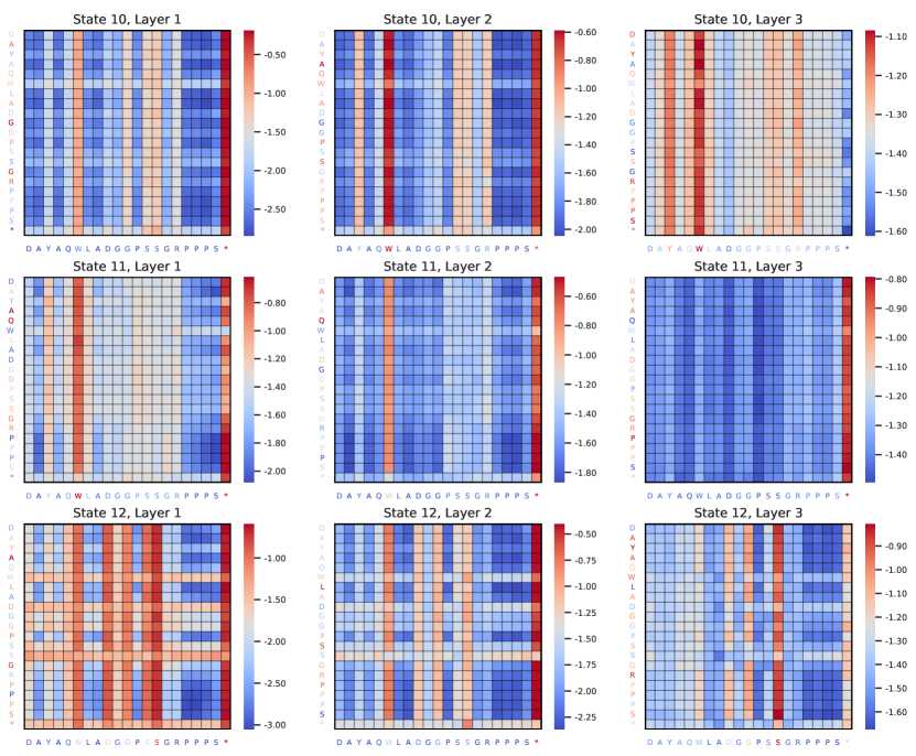
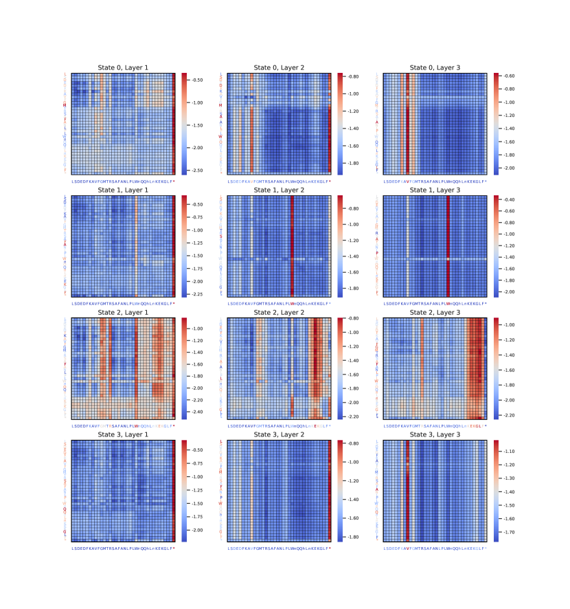
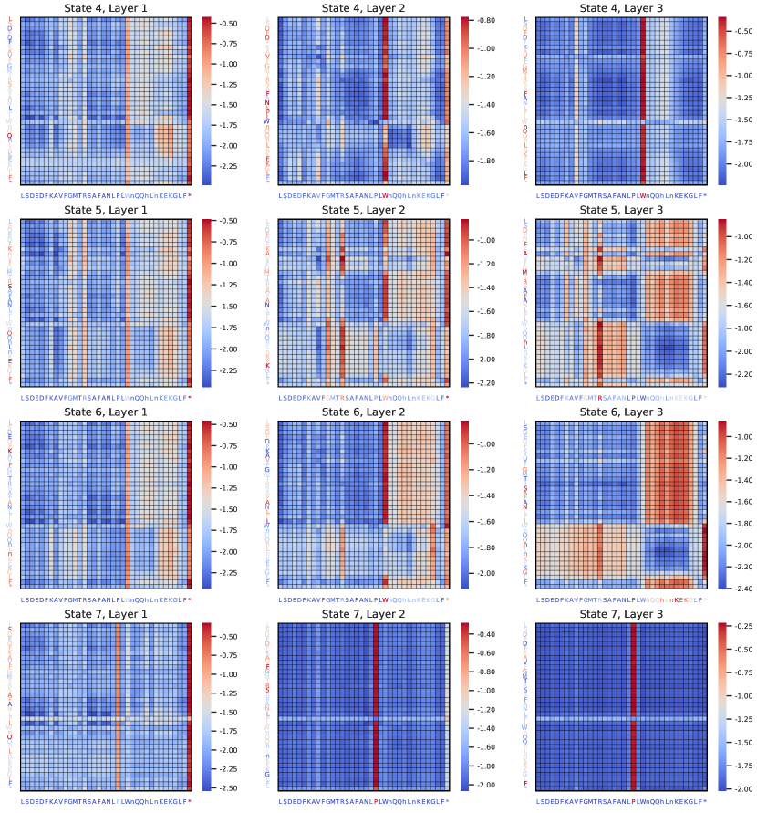
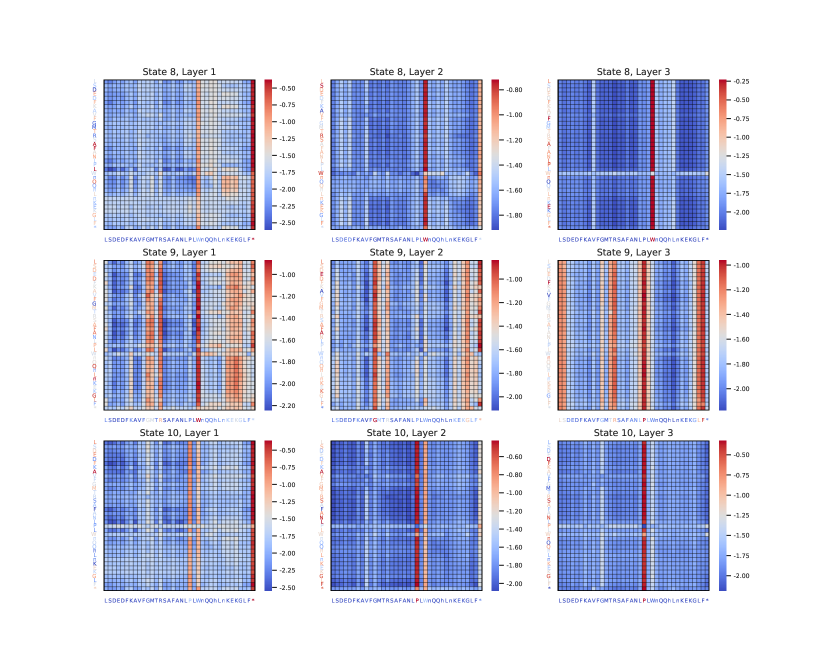
Figure S10: Log-scaled attention weight heatmaps for trp-cage SPIB states 10 to 12 from three layers of Subformer-GVP. Each subplot displays attention weights with color-coded tick labels based on normalized sums. Colorbars indicate log-scaled attention values.

Figure S11: Log-scaled attention weight heatmaps for villin SPIB states 0 to 3 from three layers of Subformer-GVP. Each subplot displays attention weights with color-coded tick labels based on normalized sums. Colorbars indicate log-scaled attention values.

The attention maps (Figure S11, S12, and S13) exhibit patterns that correspond to features of the folded structure. Notably, the attention consistently focuses on the tokens representing Val9 (V9), Gly11 (G11), Met12 (M12), Arg14 (R14), Pro21 (P21), and Trp23 (W23). These residues correspond roughly to the turns between helices. In the attention maps for states 0, 2, 5, and 6, the tokens corresponding to helix 3 feature prominently; the tokens corresponding to helix 1 are also activated in state 0. The attention maps thus suggest that the network tracks the folding and packing of the helices.

VI Computational requirements

Equivariant geometric GNNs use both invariant and equivariant features to capture the three-dimensional structure of molecules. For typical numbers of features, the memory and time requirements are expensive even for small graphs. To illustrate, we show the memory and time requirements for inference using a TorchMD-ET GNN with a small batch size with varying numbers of hidden channels (numbers of features) for trp-cage (144 non-hydrogen atoms) and villin (272 non-hydrogen atoms) in Figure S14. Even this already requires tens of gigabytes of memory and several seconds; a more complex architecture like ViSNet is expected to increase the memory and time requirements by roughly 50%. The memory and time scale linearly with both the number of atoms in the graph and the batch size. We use a batch size of 5000 for VAMP (except for GVP variants, for which we use 1000) and 1000 for SPIB, making training a GNN on the fly prohibitive, as we discuss in further detail below.

Geom2vec decouples training the GNNs and the networks for the downstream tasks. This allows us to use a small batch size for pretraining the GNNs (which need be done only once), and the networks for the downstream tasks take as inputs the tokens, which are fewer in number than the number of graph nodes. For example, here, the number of graph nodes is the number of non-hydrogen atoms, while the number of tokens is the number of amino acids, which is an order of magnitude smaller.

The computational costs training VAMPnets with different token mixers are shown in Figure 8. The simplest GNN using pooling is not much more computationally costly than an MLP that takes distances between C_α atoms as inputs. The GNNs with token mixers are about an order of magnitude more computationally costly but still manageable (hundreds of seconds) even without advanced acceleration techniques such as flash-attention or compilation. We expect the memory and computational time to scale with token number quadratically for SubFormer and subquadratically for SubMixer (depending on the expansion dimension in the token-mixing blocks).

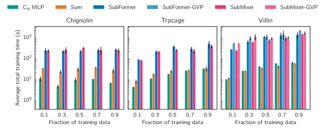
Figure 8: Computational time for training a single VAMPNet. We employ early stopping and stop training when the training VAMP score does not increase for 1000 batches or the validation VAMP score does not increase for 10 batches. Times reported are averages over three training runs, with validation performed at each step using the second half of each trajectory, as depicted in Figure S2. All times are for training on a single NVIDIA A40 GPU.

To estimate the memory usage and training time for a VAMPnet based on a GNN without pretraining, we consider a TorchMD-ET model with specific settings: a batch size of 1000, a hidden dimension of 64, and 6 layers; we assume 50 epochs are required to converge. For trp-cage, a batch size of 100 required 10.64 GB of memory. Since memory usage and training time should scale linearly with batch size, we infer that increasing the batch size to 1000 would raise the memory usage to approximately $10.64~{}\text{GB}\times 10=106.4~{}\text{GB}$. Similarly, we estimate the training time at this larger batch size to be around 1.8 hours (excluding validation). The corresponding numbers for villin, which is about twice the size, are proportionally larger (219.0 GB and 4.0 hours for training). As noted above, employing a more complex architecture like ViSNet would further increase both time and memory requirements by roughly 50%. In the present study, we actually employ a batch size of 5000 for VAMP (except for GVP variants, as noted above); we employ a batch size of 1000 for SPIB, but it generally requires more iterations to converge. While rough, these estimates show that without pretraining equivariant GNNs for analyzing molecular dynamics are beyond most researchers. By contrast, with pretraining, they are well within reach (Figures 8).

VII Conclusions

In this paper, we use pretrained GNNs to convert molecular conformations to rich vector representations that can then be used for diverse downstream tasks. Decoupling the training of the GNNs and the networks for the downstream tasks dramatically decreases the memory and computational time requirements. Here, we focused on downstream tasks concerned with analyzing dynamics in molecular simulations, specifically VAMP and SPIB. For these tasks, we were able to use equivariant GNNs that take all atoms of small proteins as inputs for the first time. The results for folding and unfolding of small proteins show that the GNNs use information beyond distances between C_α atoms, which are commonly used as input features.

For pretraining, we used a simple denoising task with a dataset of structures of diverse molecules. It would be interesting to investigate whether more complex pretraining strategies together with protein structural [72, 73] or dynamical[46] datasets can improve performance. We also explored a variety of token mixers and observed that more complex architectures were able to yield better results, which suggests there is scope for further engineering in this regard.

In our tests, we took care to split the dataset in a way that minimized the correlation between the training and validation datasets, and we believe that this should be standard practice. Because the data consisted of long, unbiased trajectories [64], there were relatively few events of interest (here, folding and unfolding). Adapting our approach to methods that take short trajectories [47, 48], which allow for greater control of sampling [47, 74], is an important area of study for the future.

Code availability

Our implementation is available at https://github.com/zpengmei/geom2vec.

References

Appendix A GNN architectures

A.1 Equivariant GNNs

Assuming $\mathbf{R}=(\mathbf{r}_{1},\mathbf{r}_{2},\ldots,\mathbf{r}_{N})\in\mathbb{R}^{3N}$ defines the molecular conformation, where $\mathbf{r}_{i}\in\mathbb{R}^{3}$ represents the 3D coordinates of the $i$-th atom, two of the most important symmetries for the GNNs to obey are translation and rigid body rotation invariance. Translation invariance and rotation invariance require that the output of the GNN, $f(\mathbf{R})$, remain unchanged when the molecule is translated by a vector $\mathbf{t}\in\mathbb{R}^{3}$, i.e., $f(\mathbf{R})=f(\mathbf{R}+\mathbf{t})$, or when the molecule undergoes a rigid body rotation represented by a rotation matrix $P\in SO(3)$, i.e., $f(\mathbf{R})=f(P\mathbf{R})$. Translation invariance can be easily realized by using the relative displacements or internal coordinates of atoms. On the other hand, rotational invariance and equivariance can be realize through either

1. a collection of scalar internal coordinates (e.g., bond distances, bond angles, and dihedral angles) to represent the atomic coordinates as in conventional classical force fields (“scalar-based network”).[75, 76, 53, 52]

2. group representation theory and spherical harmonic embedding to exploit the symmetries of the 3D rotation group $\mathrm{SO}(3)$ (“group-equivariant network”). This requires directly encoding the relative displacement vectors with spherical harmonics, which are then propagated with tensor products.[18, 19, 20]

The two approaches are theoretically and practically equivalent[77, 53, 52], but group-equivariant networks need to store the features for each irreducible representation and propagate spherical harmonic information with tensor products, making scaling in space and time to large-scale pretraining impractical. On the other hand, scalar-based networks provide a computationally efficient way to represent the conformational information of molecules while preserving the necessary invariance and equivariance properties. Therefore, we chose to employ scalar-based GNNs as a general featurizer for molecular and protein systems.

A.2 TorchMD-ET architecture

The TorchMD-ET architecture is structured around three components that process and encode molecular geometric information effectively.

1. Embedding layer: encodes atomic types and interatomic distances using exponential radial basis functions (eRBFs). Each distance $d_{ij}$ within a cutoff $r_{\text{cut}}$ is transformed by

   $$\text{eRBF}_{k}(d_{ij})=\phi(d_{ij})\exp\left(-\beta_{k}(\exp(-d_{ij})-\mu_{k})^{2}\right)$$ (S1)

   where $\phi(d_{ij})$ is a cosine cutoff function ensuring smooth transitions to zero beyond $r_{\text{cut}}$.

2. Modified attention mechanism: incorporates edge information through an extended dot-product attention that integrates interatomic distances with distance kernels $DK$ derived from eRBFs and transformed by a learned projection to influence the attention weights directly ($\odot$ denotes element-wise multiplication):

   $$A=\text{SiLU}\left(\sum_{k=1}^{F}Q_{k}\odot K_{k}\odot DK_{k}\right)\cdot\phi(d_{ij})$$ (S2)

3. Update layer: updates both scalar ($\Delta x_{i}$) and vector ($\Delta v_{i}$) features by leveraging outputs from the attention mechanism:

   $$\Delta x_{i} =q_{1i}+q_{2i}\odot(U_{1}\mathbf{v}_{i}\cdot U_{2}\mathbf{v}_{i})$$ (S3)

   $$\Delta\mathbf{v}_{i} =q_{3i}\cdot U_{3}\mathbf{v}_{i}+\sum_{j}\left(s_{1ij}\odot\mathbf{v}_{j}+s_{2ij}\odot\frac{\mathbf{r}_{i}-\mathbf{r}_{j}}{\|\mathbf{r}_{i}-\mathbf{r}_{j}\|}\right).$$ (S4)

   The $q_{\alpha i},s_{\alpha ij}\in\mathbb{R}^{F}$ are scalar features and filters obtained from the attention weights. This combines scalar and directional vector information to produce a comprehensive feature update across the molecular structure.

A.3 ViSNet

Building upon TorchMD-ET, ViSNet enhances the utilization of geometric information beyond just interatomic distances by incorporating additional scalar features such as angles and dihedrals into its architecture. ViSNet includes not only interatomic distances but also angles, dihedral angles, and improper dihedral angles. For instance, the vector rejection method helps in calculating dihedral angles:

$$\mathbf{w}_{ij}=\mathbf{v}_{i}-(\mathbf{v}_{i}\cdot\mathbf{u}_{ij})\mathbf{u}_{ij}$$ (S5)

where $\mathbf{v}_{i}$ is a vector representation of the atom $i$, and $\mathbf{u}_{ij}$ is the unit vector from atom $i$ to atom $j$. The inner product $\mathbf{w}_{ij}\cdot\mathbf{w}_{ji}$ then represents the dihedral angle information around these atoms (i.e., dihedral angles with $i$ and $j$ as the inner atoms).

ViSNet also introduced a Vector-Scalar Interactive Message Passing (ViS-MP) to fully utilize the calculated geometric features by facilitating interaction between vector and scalar representations in the network. An interaction may be described by

$$\Delta x_{i}=(W_{t}\mathbf{v}_{i}\cdot W_{s}\mathbf{v}_{i})\odot m_{i}$$ (S6)

where the scalar node embedding $x_{i}$ is updated by combining scalar messages $m_{i}$ and geometric information derived from the vectors $\mathbf{v}_{i}$.

In principle, ViSNet should be more expressive than TorchMD-ET, but we have not noticed much difference between two architectures except that TorchMD-ET is much more efficient in training/inferencing time and memory given similar model sizes.

A.4 Gated equivariant block

The output layer of the networks consists of gated equivariant blocks[78, 79], each of which combines the scalar ($x_{i}$) and vector ($\mathbf{v}_{i}$) features from graph node $i$ of the previous layer (Algorithm 1).

Algorithm 1 Gated equivariant block (GEB)

1:$x_{i}\in\mathbb{R}^{d_{i}}$, $\mathbf{v}_{i}\in\mathbb{R}^{3\times d_{i}}$

2:$v_{i}^{1},\mathbf{v}_{i}^{2}\leftarrow\|W\mathbf{v}_{i}\|,W\mathbf{v}_{i}$ $\triangleright$ $v_{i}^{1}\in\mathbb{R}^{d_{i}}$, $\mathbf{v}_{i}^{2}\in\mathbb{R}^{3\times d_{o}}$

3:$x_{i}\leftarrow[x_{i},v_{i}^{1}]$ $\triangleright$ concatenation, $x_{i}\in\mathbb{R}^{2d_{i}}$

4:$x_{i}\leftarrow W(\text{SiLU}((Wx_{i}+b)))+b$ $\triangleright$ $x_{i}\in\mathbb{R}^{2d_{o}}$

5:$[x_{i},g_{i}]\leftarrow x_{i}$ $\triangleright$ $x_{i},g_{i}\in\mathbb{R}^{d_{o}}$

6:$x_{i}\leftarrow\text{SiLU}(x_{i})$

7:$\mathbf{v}_{i}\leftarrow g_{i}\odot\mathbf{v}_{i}^{2}$ $\triangleright$ scales vector features, maintains equivariance

8:return $x_{i}$, $\mathbf{v}_{i}$ $\triangleright$ $x_{i}\in\mathbb{R}^{d_{o}}$, $\mathbf{v}_{i}\in\mathbb{R}^{3\times d_{o}}$

Appendix B Geometric vector perceptron

Geometric vector perceptron (GVP) is an equivariant GNN architecture [57] that has been used to model 3D bio-molecular structures, such as proteins. As one of the first architectures that directly incorporated vector features, GVP achieves results on difficult protein modeling tasks such as protein design that predicts amino acid sequences that fold into a given structure, and model quality assessment that evaluates the quality of predicted protein models by comparing to known structures. In the geom2vec context, we used the same architecture as an equivariant token mixer to learn how to combine both scalar and vector features (Algorithm 2).

Algorithm 2 Geometric vector perceptron (GVP)

1:$x_{i}\in\mathbb{R}^{d_{i}}$, $\mathbf{v}_{i}\in\mathbb{R}^{3\times d_{i}}$

2:$\mathbf{v}_{h}\leftarrow W_{h}\mathbf{v}_{i}$ $\triangleright$ project vector features, $\mathbf{v}_{i}\in\mathbb{R}^{3\times d_{h}}$

3:$x_{h}\leftarrow\|\mathbf{v}_{h}\|_{2}$ $\triangleright$ compute the (row-wise) scalar norm of projected vectors, $x_{h}\in\mathbb{R}^{d_{h}}$

4:$x_{h+d_{i}}\leftarrow\text{Concat}(x_{h},x_{i})$ $\triangleright$ $x_{h+d_{i}}\in\mathbb{R}^{d_{h}+d_{i}}$

5:$x_{m}\leftarrow W_{m}x_{h+d_{i}}+b_{m}$ $\triangleright$ $x_{m}\in\mathbb{R}^{d_{o}}$

6:$x^{\prime}_{i}\leftarrow\sigma(x_{m})$ $\triangleright$ $x^{\prime}_{i}\in\mathbb{R}^{d_{o}}$

7:$\mathbf{v}_{o}\leftarrow W_{o}\mathbf{v}_{h}$ $\triangleright$ project vector features to $\mathbb{R}^{3\times d_{o}}$

8:$v^{\prime}_{i}\leftarrow\sigma^{+}(\|\mathbf{v}_{o}\|_{2})$ $\triangleright$ compute the (row-wise) norm of projected vectors, $v^{\prime}_{i}\in\mathbb{R}^{d_{o}}$

9:$\mathbf{v}^{\prime}_{i}\leftarrow v^{\prime}_{i}\odot\mathbf{v}_{o}$ $\triangleright$ element-wise multiplication with norm, $\mathbf{v}^{\prime}_{i}\in\mathbb{R}^{3\times d_{o}}$

10:return $x^{\prime}_{i},\mathbf{v}^{\prime}_{i}$

Appendix C Pseudo-code of overall architecture

Algorithm 3 geom2vec

1:Atomic numbers $z_{i}$, positions $\mathbf{r}_{i}\in\mathbb{R}^{3}$ ($i=1,\dots,N$), coarse-grained mapping $\mathcal{S}=\{S_{1},\dots,S_{M}\}$, mixer method {none, subformer, submixer, subgvp}, global features $\mathbf{G}\in\mathbb{R}^{g}$

2:$x_{i}^{\text{MP}},\mathbf{v}_{i}^{\text{MP}}\leftarrow\text{MPNN}(z_{i},\mathbf{r}_{i})$ $\triangleright$ atomistic featurization, $x_{i}^{\text{MP}}\in\mathbb{R}^{d_{k}}$, $\mathbf{v}_{i}^{\text{MP}}\in\mathbb{R}^{3\times d_{k}}$

3:$x_{m}^{\text{MP}},\mathbf{v}_{m}^{\text{MP}}\leftarrow\sum_{i\in S_{m}}x_{i}^{\text{MP}},\sum_{i\in S_{m}}\mathbf{v}_{i}^{\text{MP}}$ $\triangleright$ coarse-graining with mapping $\mathcal{S}$, $x_{m}^{\text{MP}}\in\mathbb{R}^{d_{k}}$,$\mathbf{v}_{m}^{\text{MP}}\in\mathbb{R}^{3\times d_{k}}$

4:if none then

5:     $x,\mathbf{\leftarrow}\sum_{m}x_{m}^{\text{MP}},\sum_{m}\mathbf{v}_{m}^{\text{MP}}$ $\triangleright$ sum over indices $m$ for direct pooling, $x^{\text{MP}}\in\mathbb{R}^{d_{k}}$,$\mathbf{v}^{\text{MP}}\in\mathbb{R}^{3\times d_{k}}$

6:     $x,\mathbf{v}\leftarrow\text{GEB}(x^{\text{MP}})$ $\triangleright$ Algorithm 1

7:else if subformer then

8:     $x_{m},\mathbf{v}_{m}\leftarrow\text{GEB}(x_{m}^{\text{MP}},\mathbf{v}_{m}^{\text{MP}})$

9:     if global token then

10:         $g\leftarrow\text{MLP}(\mathbf{G})$ $\triangleright$ project global features $\mathbf{G}$ to $\mathbb{R}^{d_{k}}$

11:         $x^{g}_{m}\leftarrow\text{Concat}(x_{m},g)$ $\triangleright$ concatenate the global token with the regular tokens

12:         $x\leftarrow\text{TransformerEncoder}(x^{g}_{m})$ $\triangleright$ pass concatenated tokens through the Transformer encoder

13:     else

14:         $x\leftarrow\text{TransformerEncoder}(x_{m})$ $\triangleright$ pass only the regular tokens through the Transformer encoder

15:     end if

16:else if submixer then

17:     $x_{m},\mathbf{v}_{m}\leftarrow\text{GEB}(x_{m}^{\text{MP}},\mathbf{v}_{m}^{\text{MP}})$ $\triangleright$ apply GEB to input features

18:     if global token then

19:         $g\leftarrow\text{MLP}(\mathbf{G})$ $\triangleright$ project global features $\mathbf{G}$ to $\mathbb{R}^{d_{k}}$

20:         $x^{g}_{m}\leftarrow\text{Concat}(x_{m},g)$ $\triangleright$ concatenate the global token with the regular tokens

21:         $x\leftarrow\text{MLPMixer}(x^{g}_{m})$ $\triangleright$ pass concatenated tokens through the MLP-Mixer

22:     else

23:         $x\leftarrow\text{MLPMixer}(x_{m})$ $\triangleright$ pass only the regular tokens through the MLP-Mixer

24:     end if

25:else if subgvp then

26:     $x_{m}^{\text{GVP}},\mathbf{v}_{m}^{\text{GVP}}\leftarrow\text{GVP}(x_{m}^{\text{MP}},\mathbf{v}_{m}^{\text{MP}})$ $\triangleright$ Algorithm 2

27:     if post mixing then

28:         $x\leftarrow\text{subformer or submixer}(x_{m}^{\text{GVP}})$ $\triangleright$ apply subformer or submixer block to transform GVP features

29:     end if

30:end if

31:$x\leftarrow\text{MLP}(x)$

32:return $x$ $\triangleright$ $x\in\mathbb{R}^{d_{o}}$

Appendix D Training details and hyperparameters

We uses the Denali dataset from ref. 43, which consists of 2.3 million 3-D conformations of small to medium size molecules. These conformations are obtained with semi-empirical methods and contain non-equilibrium geometries, alternative tautomers, and non-bonded interactions. For pretraining, we randomly take 10,000 configurations as validation set and the remaining as training set.

Table S1: Hyperparameters for pretrained networks (TorchMD-ET and ViSNet)

Hyperparameter	TorchMD-ET and ViSNet
Hidden dimension ($d$)	64, 128, 256, 384
# of MP layers	6
# of attention heads	8
Batch size	100
Epochs	10
# of RBFs	64
$r_{\mathrm{cut}}$ (Å)	5, 7.5
Learning rate	0.0005
Optimizer	AdamW (AMSGrad)
Noise level	0.2

Table S2: Hyperparameters for VAMPnets with pretrained GNN

Hyperparameter	Chignolin	Villin	Trp-cage
Batch size	5000	5000/1000	5000/1000
Learning rate	0.0002	0.0002	0.0002
Optimizer	AdamAtan2	AdamAtan2	AdamAtan2
Maximum epochs	20	20	20
Training patience	10	10	10
Validation patience	2	2	2
Validation interval	5	5/20	5
MLP hidden dimension	256	128	128
MLP activation function	SiLU	SiLU	SiLU
Trajectory stride	1	2	4
Training lag time (ns)	4	20	10
$d$	256	128/64	128/64
Dropout	0.2	0.2	0.2
BatchNorm	False	False	False
Output dimension ($k$)	2	3	4

Table S3: Hyperparameters for SPIB with pretrained GNN

Hyperparameter	Villin	Trp-cage
Batch size	1000	1000
Learning rate	0.0002	0.0002
Optimizer	AdamAtan2	AdamAtan2
Training patience	5	5
Label refinement	5	5
MLP hidden dimension	64	64
MLP activation function	SiLU	SiLU
Trajectory stride	2	4
Training lag time (ns)	20	10
$d$	64	64
Dropout	0.2	0.2
BatchNorm	False	False

Appendix E Supplementary Figures

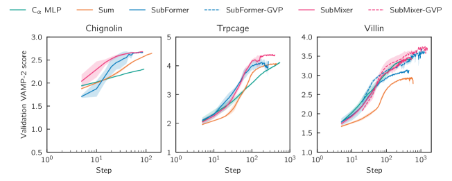
Figure S2: Validation curves for VAMPnets on all three systems and all three mixers studied. Each curve represents the mean of three training runs. Shaded regions indicate standard error over three runs.

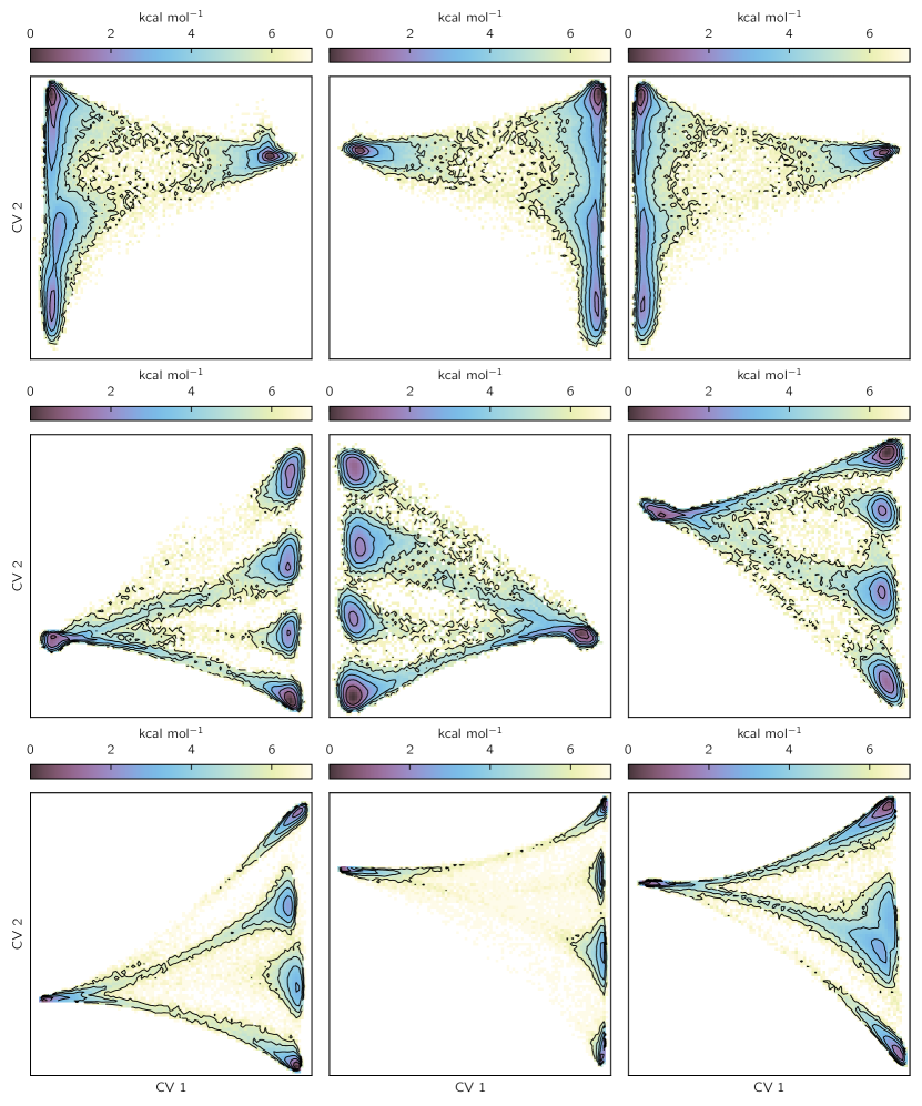
Figure S3: PMFs as a function of VAMP CVs for chignolin. From top to bottom, VAMPnets were trained with no mixer (C_α MLP), SubMixer, or SubFormer. Each column shows the result from a single training run. Contours are drawn every 1 kcal/mol.

Figure S4: PMFs as a function of VAMP CVs for trp-cage. From top to bottom, VAMPnets were trained with no mixer (C_α MLP), SubMixer, or SubFormer. Each column shows the result from a single training run. Contours are drawn every 1 kcal/mol.

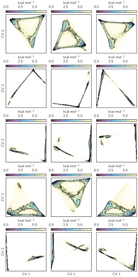
Figure S5: PMFs as a function of VAMP CVs for villin. From top to bottom, VAMPnets were trained with no mixer (C_α MLP), SubMixer, SubMixer-GVP, SubFormer, or SubFormer-GVP. Each column shows the result from a single training run. Contours are drawn every 1 kcal/mol.

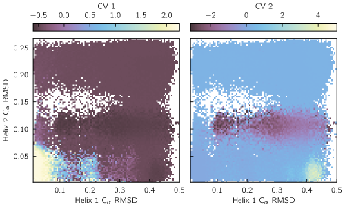
Figure S6: Trp-cage VAMPnet (with SubMixer) CVs as a function of two physical coordinates: C_α RMSD of helix 1 and C_α RMSD of helix 2.

Figure S7: Villin VAMPnet (with SubFormer) CVs as a function of two physical coordinates: C_α RMSD of helices 1 and 2, and C_α RMSD of helices 2 and 3.

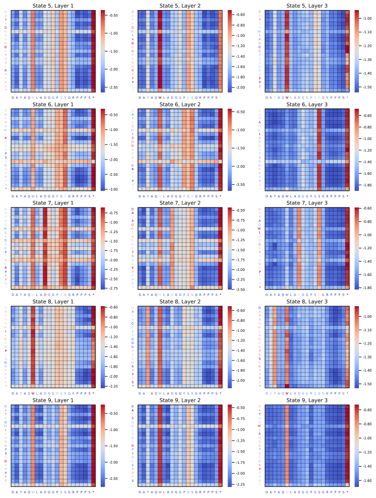
Figure S9: Log-scaled attention weight heatmaps for trp-cage SPIB states 5 to 9 from three layers of Subformer-GVP. Each subplot displays attention weights with color-coded tick labels based on normalized sums. Colorbars indicate log-scaled attention values.

Figure S12: Log-scaled attention weight heatmaps for villin SPIB states 4 to 7 from three layers of Subformer-GVP. Each subplot displays attention weights with color-coded tick labels based on normalized sums. Colorbars indicate log-scaled attention values.

Figure S13: Log-scaled attention weight heatmaps for villin SPIB states 8 to 10 from three layers of Subformer-GVP. Each subplot displays attention weights with color-coded tick labels based on normalized sums. Colorbars indicate log-scaled attention values.

Figure S14: Comparison of time and GPU memory usage of TorchMD-ET in training and inference modes on the trp-cage (left) and villin (right) subsets, each consisting of 2000 frames with 100 frames per batch. The measurements are done without specific objective functions for usage benchmarking purpose. The model’s performance is evaluated across varying numbers of hidden channels (64, 128, 256, 384) and layers (1–6). The heatmaps on the left show GPU memory allocated in gigabytes (GB), while the heatmaps on the right depict time usage in seconds. The time represents one forward pass for inference mode and one forward plus one backward pass for training mode. Measurements were performed on an NVIDIA A100 40G GPU. Missing values are due to out-of-memory errors for certain configurations.

References

- Husic et al. [2016] B. E. Husic, R. T. McGibbon, M. M. Sultan, and V. S. Pande, “Optimized parameter selection reveals trends in Markov state models for protein folding,” The Journal of Chemical Physics 145, 194103 (2016).
- Scherer et al. [2019] M. K. Scherer, B. E. Husic, M. Hoffmann, F. Paul, H. Wu, and F. Noé, “Variational selection of features for molecular kinetics,” The Journal of Chemical Physics 150, 194108 (2019).
- Nagel, Sartore, and Stock [2023] D. Nagel, S. Sartore, and G. Stock, “Selecting Features for Markov Modeling: A Case Study on HP35,” Journal of Chemical Theory and Computation (2023), 10.1021/acs.jctc.3c00240.
- Arbon, Zhu, and Mey [2024] R. E. Arbon, Y. Zhu, and A. S. J. S. Mey, “Markov State Models: To Optimize or Not to Optimize,” Journal of Chemical Theory and Computation 20, 977–988 (2024).
- Tribello, Ceriotti, and Parrinello [2012] G. A. Tribello, M. Ceriotti, and M. Parrinello, “Using sketch-map coordinates to analyze and bias molecular dynamics simulations,” Proceedings of the National Academy of Sciences 109, 5196–5201 (2012).
- Rohrdanz et al. [2011] M. A. Rohrdanz, W. Zheng, M. Maggioni, and C. Clementi, “Determination of reaction coordinates via locally scaled diffusion map,” The Journal of Chemical Physics 134, 124116 (2011).
- Boninsegna et al. [2015] L. Boninsegna, G. Gobbo, F. Noé, and C. Clementi, “Investigating Molecular Kinetics by Variationally Optimized Diffusion Maps,” Journal of Chemical Theory and Computation 11, 5947–5960 (2015).
- Mardt et al. [2018] A. Mardt, L. Pasquali, H. Wu, and F. Noé, “VAMPnets for deep learning of molecular kinetics,” Nature Communications 9, 5 (2018).
- Noé and Nüske [2013] F. Noé and F. Nüske, “A Variational Approach to Modeling Slow Processes in Stochastic Dynamical Systems,” Multiscale Modeling & Simulation 11, 635–655 (2013).
- Wu and Noé [2020] H. Wu and F. Noé, “Variational Approach for Learning Markov Processes from Time Series Data,” Journal of Nonlinear Science 30, 23–66 (2020).
- Lorpaiboon et al. [2020] C. Lorpaiboon, E. H. Thiede, R. J. Webber, J. Weare, and A. R. Dinner, “Integrated Variational Approach to Conformational Dynamics: A Robust Strategy for Identifying Eigenfunctions of Dynamical Operators,” The Journal of Physical Chemistry B 124, 9354–9364 (2020).
- Trstanova, Leimkuhler, and Lelièvre [2020] Z. Trstanova, B. Leimkuhler, and T. Lelièvre, “Local and global perspectives on diffusion maps in the analysis of molecular systems,” Proceedings of the Royal Society A 476, 20190036 (2020).
- Strahan et al. [2021] J. Strahan, A. Antoszewski, C. Lorpaiboon, B. P. Vani, J. Weare, and A. R. Dinner, “Long-Time-Scale Predictions from Short-Trajectory Data: A Benchmark Analysis of the Trp-Cage Miniprotein,” Journal of Chemical Theory and Computation 17, 2948–2963 (2021).
- Thiede et al. [2019] E. H. Thiede, D. Giannakis, A. R. Dinner, and J. Weare, “Galerkin Approximation of Dynamical Quantities using Trajectory Data,” The Journal of Chemical Physics 150, 244111 (2019).
- Ma and Dinner [2005] A. Ma and A. R. Dinner, “Automatic Method for Identifying Reaction Coordinates in Complex Systems,” The Journal of Physical Chemistry B 109, 6769–6779 (2005).
- Guo et al. [2024] S. C. Guo, R. Shen, B. Roux, and A. R. Dinner, “Dynamics of activation in the voltage-sensing domain of Ciona intestinalis phosphatase Ci-VSP,” Nature Communications 15, 1408 (2024).
- Herringer et al. [2023] N. S. Herringer, S. Dasetty, D. Gandhi, J. Lee, and A. L. Ferguson, “Permutationally invariant networks for enhanced sampling (pines): Discovery of multimolecular and solvent-inclusive collective variables,” Journal of Chemical Theory and Computation 20, 178–198 (2023).
- Thomas et al. [2018] N. Thomas, T. Smidt, S. Kearnes, L. Yang, L. Li, K. Kohlhoff, and P. Riley, “Tensor field networks: Rotation-and translation-equivariant neural networks for 3d point clouds,” arXiv preprint arXiv:1802.08219 (2018).
- Anderson, Hy, and Kondor [2019] B. Anderson, T. S. Hy, and R. Kondor, “Cormorant: Covariant molecular neural networks,” Advances in neural information processing systems 32 (2019).
- Batzner et al. [2022] S. Batzner, A. Musaelian, L. Sun, M. Geiger, J. P. Mailoa, M. Kornbluth, N. Molinari, T. E. Smidt, and B. Kozinsky, “E(3)-equivariant graph neural networks for data-efficient and accurate interatomic potentials,” Nature communications 13, 2453 (2022).
- Gilmer et al. [2017] J. Gilmer, S. S. Schoenholz, P. F. Riley, O. Vinyals, and G. E. Dahl, “Neural message passing for quantum chemistry,” in International conference on machine learning (PMLR, 2017) pp. 1263–1272.
- Battaglia et al. [2018] P. W. Battaglia, J. B. Hamrick, V. Bapst, A. Sanchez-Gonzalez, V. Zambaldi, M. Malinowski, A. Tacchetti, D. Raposo, A. Santoro, R. Faulkner, C. Gulcehre, F. Song, A. Ballard, J. Gilmer, G. Dahl, A. Vaswani, K. Allen, C. Nash, V. Langston, C. Dyer, N. Heess, D. Wierstra, P. Kohli, M. Botvinick, O. Vinyals, Y. Li, and R. Pascanu, “Relational inductive biases, deep learning, and graph networks,” (2018), arXiv:1806.01261 [cs, stat].
- Husic et al. [2020] B. E. Husic, N. E. Charron, D. Lemm, J. Wang, A. Pérez, M. Majewski, A. Krämer, Y. Chen, S. Olsson, G. de Fabritiis, et al., “Coarse graining molecular dynamics with graph neural networks,” The Journal of chemical physics 153 (2020).
- Han et al. [2024] J. Han, J. Cen, L. Wu, Z. Li, X. Kong, R. Jiao, Z. Yu, T. Xu, F. Wu, Z. Wang, et al., “A survey of geometric graph neural networks: Data structures, models and applications,” arXiv preprint arXiv:2403.00485 (2024).
- Jamasb et al. [2023] A. R. Jamasb, A. Morehead, Z. Zhang, C. K. Joshi, K. Didi, S. V. Mathis, C. Harris, J. Tang, J. Cheng, P. Lio, and T. L. Blundell, “Evaluating Representation Learning on the Protein Structure Universe,” in The Twelfth International Conference on Learning Representations (2023).
- Hermosilla and Ropinski [2022] P. Hermosilla and T. Ropinski, “Contrastive Representation Learning for 3D Protein Structures,” (2022), arXiv:2205.15675 [cs, q-bio].
- Wang et al. [2023] L. Wang, H. Liu, Y. Liu, J. Kurtin, and S. Ji, “Learning Hierarchical Protein Representations via Complete 3D Graph Networks,” (2023), arXiv:2207.12600 [cs, q-bio].
- Zhang et al. [2023] Z. Zhang, M. Xu, A. Jamasb, V. Chenthamarakshan, A. Lozano, P. Das, and J. Tang, “Protein Representation Learning by Geometric Structure Pretraining,” (2023), arXiv:2203.06125 [cs].
- Baek et al. [2021] M. Baek, F. DiMaio, I. Anishchenko, J. Dauparas, S. Ovchinnikov, G. R. Lee, J. Wang, Q. Cong, L. N. Kinch, R. D. Schaeffer, C. Millán, H. Park, C. Adams, C. R. Glassman, A. DeGiovanni, J. H. Pereira, A. V. Rodrigues, A. A. v. Dijk, A. C. Ebrecht, D. J. Opperman, T. Sagmeister, C. Buhlheller, T. Pavkov-Keller, M. K. Rathinaswamy, U. Dalwadi, C. K. Yip, J. E. Burke, K. C. Garcia, N. V. Grishin, P. D. Adams, R. J. Read, and D. Baker, “Accurate prediction of protein structures and interactions using a three-track neural network,” Science (2021), 10.1126/science.abj8754.
- Xie et al. [2019] T. Xie, A. France-Lanord, Y. Wang, Y. Shao-Horn, and J. C. Grossman, “Graph dynamical networks for unsupervised learning of atomic scale dynamics in materials,” Nature communications 10, 2667 (2019).
- Soltani, Sinclair, and Rottler [2022] S. Soltani, C. W. Sinclair, and J. Rottler, “Exploring glassy dynamics with markov state models from graph dynamical neural networks,” Physical Review E 106, 025308 (2022).
- Ghorbani et al. [2022] M. Ghorbani, S. Prasad, J. B. Klauda, and B. R. Brooks, “Graphvampnet, using graph neural networks and variational approach to markov processes for dynamical modeling of biomolecules,” The Journal of Chemical Physics 156 (2022).
- Liu et al. [2023] B. Liu, M. Xue, Y. Qiu, K. A. Konovalov, M. S. O’Connor, and X. Huang, “Graphvampnets for uncovering slow collective variables of self-assembly dynamics,” The Journal of Chemical Physics 159 (2023).
- Huang et al. [2024] Y. Huang, H. Zhang, Z. Lin, Y. Wei, and W. Xi, “Revgraphvamp: A protein molecular simulation analysis model combining graph convolutional neural networks and physical constraints,” bioRxiv , 2024–03 (2024).
- Vaswani et al. [2017] A. Vaswani, N. Shazeer, N. Parmar, J. Uszkoreit, L. Jones, A. N. Gomez, Ł. Kaiser, and I. Polosukhin, “Attention is all you need,” Advances in neural information processing systems 30 (2017).
- Dosovitskiy et al. [2020] A. Dosovitskiy, L. Beyer, A. Kolesnikov, D. Weissenborn, X. Zhai, T. Unterthiner, M. Dehghani, M. Minderer, G. Heigold, S. Gelly, et al., “An image is worth 16x16 words: Transformers for image recognition at scale,” arXiv preprint arXiv:2010.11929 (2020).
- Mikolov et al. [2013] T. Mikolov, I. Sutskever, K. Chen, G. S. Corrado, and J. Dean, “Distributed representations of words and phrases and their compositionality,” Advances in neural information processing systems 26 (2013).
- Guo et al. [2022] Y. Guo, J. Wu, H. Ma, and J. Huang, “Self-supervised pre-training for protein embeddings using tertiary structures,” in Proceedings of the AAAI conference on artificial intelligence, Vol. 36 (2022) pp. 6801–6809.
- Chen et al. [2023] C. Chen, J. Zhou, F. Wang, X. Liu, and D. Dou, “Structure-aware protein self-supervised learning,” Bioinformatics 39, btad189 (2023).
- Zaidi et al. [2022] S. Zaidi, M. Schaarschmidt, J. Martens, H. Kim, Y. W. Teh, A. Sanchez-Gonzalez, P. Battaglia, R. Pascanu, and J. Godwin, “Pre-training via denoising for molecular property prediction,” arXiv preprint arXiv:2206.00133 (2022).
- Sohl-Dickstein et al. [2015] J. Sohl-Dickstein, E. Weiss, N. Maheswaranathan, and S. Ganguli, “Deep unsupervised learning using nonequilibrium thermodynamics,” in International conference on machine learning (PMLR, 2015) pp. 2256–2265.
- Song, Meng, and Ermon [2020] J. Song, C. Meng, and S. Ermon, “Denoising diffusion implicit models,” arXiv preprint arXiv:2010.02502 (2020).
- Christensen et al. [2021] A. S. Christensen, S. K. Sirumalla, Z. Qiao, M. B. O’Connor, D. G. Smith, F. Ding, P. J. Bygrave, A. Anandkumar, M. Welborn, F. R. Manby, et al., “OrbNet Denali: A machine learning potential for biological and organic chemistry with semi-empirical cost and DFT accuracy,” The Journal of Chemical Physics 155 (2021).
- Wang and Tiwary [2021a] D. Wang and P. Tiwary, “State predictive information bottleneck,” The Journal of Chemical Physics 154 (2021a).
- Wang et al. [2024a] D. Wang, Y. Qiu, E. R. Beyerle, X. Huang, and P. Tiwary, “Information bottleneck approach for markov model construction,” Journal of Chemical Theory and Computation (2024a).
- Vander Meersche et al. [2024] Y. Vander Meersche, G. Cretin, A. Gheeraert, J.-C. Gelly, and T. Galochkina, “ATLAS: protein flexibility description from atomistic molecular dynamics simulations,” Nucleic Acids Research 52, D384–D392 (2024).
- Strahan et al. [2023a] J. Strahan, J. Finkel, A. R. Dinner, and J. Weare, “Predicting rare events using neural networks and short-trajectory data,” Journal of computational physics 488, 112152 (2023a).
- Strahan et al. [2023b] J. Strahan, S. C. Guo, C. Lorpaiboon, A. R. Dinner, and J. Weare, “Inexact iterative numerical linear algebra for neural network-based spectral estimation and rare-event prediction,” The Journal of Chemical Physics 159, 014110 (2023b).
- Jung et al. [2023] H. Jung, R. Covino, A. Arjun, C. Leitold, C. Dellago, P. G. Bolhuis, and G. Hummer, “Machine-guided path sampling to discover mechanisms of molecular self-organization,” Nature Computational Science 3, 334–345 (2023).
- Bonati, Piccini, and Parrinello [2021] L. Bonati, G. Piccini, and M. Parrinello, “Deep learning the slow modes for rare events sampling,” Proceedings of the National Academy of Sciences 118 (2021), 10.1073/pnas.2113533118.
- Hernández et al. [2018] C. X. Hernández, H. K. Wayment-Steele, M. M. Sultan, B. E. Husic, and V. S. Pande, “Variational encoding of complex dynamics,” Physical Review E 97, 062412 (2018).
- Wang et al. [2024b] Y. Wang, T. Wang, S. Li, X. He, M. Li, Z. Wang, N. Zheng, B. Shao, and T.-Y. Liu, “Enhancing geometric representations for molecules with equivariant vector-scalar interactive message passing,” Nature Communications 15, 313 (2024b).
- Thölke and De Fabritiis [2022] P. Thölke and G. De Fabritiis, “Torchmd-net: Equivariant transformers for neural network based molecular potentials,” arXiv preprint arXiv:2202.02541 (2022).
- Carion et al. [2020] N. Carion, F. Massa, G. Synnaeve, N. Usunier, A. Kirillov, and S. Zagoruyko, “End-to-end object detection with transformers,” in European conference on computer vision (Springer, 2020) pp. 213–229.
- Tolstikhin et al. [2021] I. O. Tolstikhin, N. Houlsby, A. Kolesnikov, L. Beyer, X. Zhai, T. Unterthiner, J. Yung, A. Steiner, D. Keysers, J. Uszkoreit, et al., “Mlp-mixer: An all-mlp architecture for vision,” Advances in neural information processing systems 34, 24261–24272 (2021).
- Pengmei et al. [2023] Z. Pengmei, Z. Li, C. chan Tien, R. Kondor, and A. Dinner, “Transformers are efficient hierarchical chemical graph learners,” in NeurIPS 2023 AI for Science Workshop (2023).
- Jing et al. [2020] B. Jing, S. Eismann, P. Suriana, R. J. L. Townshend, and R. Dror, “Learning from protein structure with geometric vector perceptrons,” in International Conference on Learning Representations (2020).
- Pengmei and Li [2024] Z. Pengmei and Z. Li, “Technical report: The graph spectral token – enhancing graph transformers with spectral information,” (2024), arXiv:2404.05604 [cs.LG] .
- Williams, Kevrekidis, and Rowley [2015] M. O. Williams, I. G. Kevrekidis, and C. W. Rowley, “A Data–Driven Approximation of the Koopman Operator: Extending Dynamic Mode Decomposition,” Journal of Nonlinear Science 25, 1307–1346 (2015).
- Nuske et al. [2014] F. Nuske, B. G. Keller, G. Pérez-Hernández, A. S. Mey, and F. Noé, “Variational approach to molecular kinetics,” Journal of chemical theory and computation 10, 1739–1752 (2014).
- Lorpaiboon et al. [2023] C. Lorpaiboon, S. C. Guo, J. Strahan, J. Weare, and A. R. Dinner, “Accurate estimates of dynamical statistics using memory,” (2023).
- Wang and Tiwary [2021b] D. Wang and P. Tiwary, “State predictive information bottleneck,” The Journal of Chemical Physics 154, 134111 (2021b).
- Tomczak and Welling [2018] J. Tomczak and M. Welling, “Vae with a vampprior,” in International conference on artificial intelligence and statistics (PMLR, 2018) pp. 1214–1223.
- Lindorff-Larsen et al. [2011] K. Lindorff-Larsen, S. Piana, R. O. Dror, and D. E. Shaw, “How Fast-Folding Proteins Fold,” Science 334, 517–520 (2011).
- Sidky, Chen, and Ferguson [2019] H. Sidky, W. Chen, and A. L. Ferguson, “High-resolution markov state models for the dynamics of trp-cage miniprotein constructed over slow folding modes identified by state-free reversible vampnets,” The Journal of Physical Chemistry B 123, 7999–8009 (2019).
- McKnight et al. [1996] J. C. McKnight, D. S. Doering, P. T. Matsudaira, and P. S. Kim, “A Thermostable 35-Residue Subdomain within Villin Headpiece,” Journal of Molecular Biology 260, 126–134 (1996).
- Kubelka et al. [2006] J. Kubelka, T. K. Chiu, D. R. Davies, W. A. Eaton, and J. Hofrichter, “Sub-microsecond Protein Folding,” Journal of Molecular Biology 359, 546–553 (2006).
- Wang et al. [2019] E. Wang, P. Tao, J. Wang, and Y. Xiao, “A novel folding pathway of the villin headpiece subdomain HP35,” Physical Chemistry Chemical Physics 21, 18219–18226 (2019).
- Chen, Roux, and Chipot [2023] H. Chen, B. Roux, and C. Chipot, “Discovering Reaction Pathways, Slow Variables, and Committor Probabilities with Machine Learning,” Journal of Chemical Theory and Computation 19, 4414–4426 (2023).
- Honda et al. [2008] S. Honda, T. Akiba, Y. S. Kato, Y. Sawada, M. Sekijima, M. Ishimura, A. Ooishi, H. Watanabe, T. Odahara, and K. Harata, “Crystal structure of a ten-amino acid protein,” Journal of the American Chemical Society 130, 15327–15331 (2008).
- Chennakesavalu, Toomer, and Rotskoff [2023] S. Chennakesavalu, D. J. Toomer, and G. M. Rotskoff, “Ensuring thermodynamic consistency with invertible coarse-graining,” The Journal of Chemical Physics 158, 124126 (2023).
- Sillitoe et al. [2021] I. Sillitoe, N. Bordin, N. Dawson, V. P. Waman, P. Ashford, H. M. Scholes, C. S. M. Pang, L. Woodridge, C. Rauer, N. Sen, M. Abbasian, S. Le Cornu, S. D. Lam, K. Berka, I. Varekova, R. Svobodova, J. Lees, and C. A. Orengo, “CATH: increased structural coverage of functional space,” Nucleic Acids Research 49, D266–D273 (2021).
- Barrio-Hernandez et al. [2023] I. Barrio-Hernandez, J. Yeo, J. Jänes, M. Mirdita, C. L. M. Gilchrist, T. Wein, M. Varadi, S. Velankar, P. Beltrao, and M. Steinegger, “Clustering predicted structures at the scale of the known protein universe,” Nature 622, 637–645 (2023).
- Strahan et al. [2024] J. Strahan, C. Lorpaiboon, J. Weare, and A. R. Dinner, “Bad-neus: Rapidly converging trajectory stratification,” The Journal of Chemical Physics 161 (2024).
- Schütt et al. [2018] K. T. Schütt, H. E. Sauceda, P.-J. Kindermans, A. Tkatchenko, and K.-R. Müller, “Schnet–a deep learning architecture for molecules and materials,” The Journal of Chemical Physics 148 (2018).
- Gasteiger, Groß, and Günnemann [2020] J. Gasteiger, J. Groß, and S. Günnemann, “Directional message passing for molecular graphs,” arXiv preprint arXiv:2003.03123 (2020).
- Villar et al. [2021] S. Villar, D. W. Hogg, K. Storey-Fisher, W. Yao, and B. Blum-Smith, “Scalars are universal: Equivariant machine learning, structured like classical physics,” Advances in Neural Information Processing Systems 34, 28848–28863 (2021).
- Weiler et al. [2018] M. Weiler, M. Geiger, M. Welling, W. Boomsma, and T. S. Cohen, “3D Steerable CNNs: Learning Rotationally Equivariant Features in Volumetric Data,” in Advances in Neural Information Processing Systems, Vol. 31 (Curran Associates, Inc., 2018).
- Schütt, Unke, and Gastegger [2021] K. T. Schütt, O. T. Unke, and M. Gastegger, “Equivariant message passing for the prediction of tensorial properties and molecular spectra,” (2021), arXiv:2102.03150 [physics].