Pickleball Flight Dynamics
Abstract
This paper considers the flight dynamics of the ball in the sport of pickleball. Various simplifications are introduced according to the features of the game. These simplifications and some approximations enable straightforward coding to study aspects of the game such as the trajectory of the ball and its velocity. In turn, strategic questions may be addressed that have not been previously considered. In particular, our primary research question involves the preference between playing with the wind versus against the wind. It is demonstrated that playing against the wind is often preferable than playing with the wind.
Keywords: pickleball, projectile motion, strategy.
1 INTRODUCTION
Pickleball is a relatively new sport. It was invented in 1985, and in recent years its popularity has taken off. Pickleball was the fastest growing sport from 2022 to 2023 in the United States with over 8.9 million participants [1]. According to a 2023 report from the Association of Pickleball Players (APP), nearly 50 million Americans have played pickleball at least once in the previous year (https://www.theapp.global). The game is popular across wide age cohorts at the recreational level. Pickleball also has various professional leagues and tours including Major League Pickleball (MLP).
Despite the popularity of the sport, there has been little quantitative research on pickleball. [5] consider the impact of strong and weak links on success in doubles pickleball. It is the intention of this paper to add to the sparse literature with a specific aim of gaining a better understanding of pickleball flight dynamics. [2] consider problems in sports analytics across major sports.
The topic of projectile motion has a long and well-studied history [6]. The details are complex, especially when considerations are given to the impact of air resistance and wind. Projectile motion models typically involve special functions and differential equations. Such work is important to serious investigations such as ballistics. In sport, [3] considers issues of approximate projectile motion in the sports of golf, tennis and badminton. However, there does not seem to be any literature on pickleball flight dynamics; this paper attempts to provide some initial insights on this topic.
In the problem considered here, we take features of the sport of pickleball into account. This, together with additional assumptions simplifies our projectile motion model. The final model is straightforward to code so that various investigations involving pickleball may be undertaken. In particular, we look at the impact of the wind in pickleball. Pickleball is often played outdoors where the choice of ends, and understanding how to play in the wind become issues of strategy. Our primary research question involves the preference between playing with the wind versus playing against the wind where it is demonstrated that playing against the wind is preferable in many contexts. This problem in pickleball strategy does not seem to have been previously addressed.
In Section 2, we provide a description of the relevant details of the pickleball court, and features of interest. We also define the relevant input variables to the projectile motion model. In Section 3, the basics of the pickleball motion model are described. In particular, we explain how features and strategies in the sport allow us to calculate input variables that are not immediately available. In Section 4, we look at various pickleball applications. In particular, we investigate pickleball trajectory and pickleball velocity under various conditions. We then discuss a question of strategy in terms of whether it is better to play against the wind or with the wind. The work indicates that a strategic advantage is often conferred when playing against the wind. We conclude with a short discussion in Section 5. Details regarding modelling and simulations are left to the Appendix.
2 PROBLEM FORMULATION
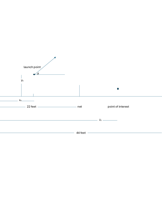
Figure 1 provides the relevant details of the pickleball court and features of interest. The pickleball court is 44 feet long which is divided into two equal halves by a net. The net is 3 feet tall at the ends although this detail is not important for our motion model.
In Figure 1, a launch point is depicted on the left side of the court. This is the location from which the player of interest strikes the pickleball. The location is marked feet from the left endline and serves as an input variable for our investigation. We have the constraint feet where we note that the 15 foot mark denotes the beginning of the non-volley zone (i.e. the closest point to the net that the player should approach). The player strikes the ball at height . We consider feet as a range for the height at which the pickleball is struck. Although the pickleball can be struck from higher heights, this range corresponds to the situation where the ball is hit in an upwards trajectory. Further, the ball is struck at launch angle . For our purposes, we consider . An angle larger than either represents a lob shot or a mishit, two shots that are not relevant to this investigation.
In Figure 1, we also depict the opponent (i.e. the point of interest) on the right side of the court whose horizontal position is given by feet from the left endline. Later, we are interested in the opponent’s ability to hit the struck ball. Since the opponent is not advised to stand in his non-volley zone, we have the constraint .
There are two quantities that are relevant to our investigation that are not depicted in Figure 1. First, the wind is a characteristic of interest. We make the assumption that the wind blows in a strictly horizontal direction. Our personal experiences in pickleball suggest that playing in winds which are less than 10 mph is largely inconsequential. On the other hand, playing in wind speeds exceeding 20 mph is extreme and is a situation that many players avoid. Therefore, we are interested in wind velocities (i.e. speed and direction) in the intermediate intervals mph and mph.
Second, we require the initial velocity which is velocity that the pickleball is struck at the launch point. In the related sport of tennis, the average serve in men’s professional tennis (e.g. the ATP tour) is estimated at 120 mph. Unlike tennis, the pickleball paddle is rigid (without strings), and the ball is hard and compresses only negligibly. Therefore, the fastest pickleball shots reach instantaneous speeds of roughly 60 mph.
Therefore, to summarize, the input variables that are relevant to pickleball flight dynamics are .
3 PICKLEBALL MOTION MODEL
This section describes the basics of the pickleball motion model. More details including the associated physics of the model are provided in the Appendix.
For this investigation, it is convenient to express the location and the speed of the pickleball in both the and coordinates. We denote the location and speed of the pickleball by and in the horizontal direction, and by and in the vertical direction.
Referring back to the discussion and the notation in Section 1, the coordinate speeds are expressed more fully as
| (1) |
The arguments of the speeds in (1) have common terms, namely the time from launch , the launch angle , the wind velocity and the initial velocity . Of course, and as described in the Appendix, the functions in (1) also depend on the features of the pickleball (e.g. weight, size and surface) which determine the impact of air resistance. Also, the force of gravity comes into play in the vertical speed but not in the horizontal speed. In our model, we ignore the impact of spin.
In (1) we note that the speed functions depend on the launch angle and the initial velocity . Since the initial coordinate speeds only depend on and through the initial coordinate speeds, using trigonometry in (1), we may replace and in by , and we may replace and in by . However, we retain the excessive notation in (1) which is helpful in future considerations.
For the coordinate locations, these are expressed more fully as
| (2) |
The functions in (2) have the same arguments as in (1) except that the initial locations and also influence location at time .
It may be noted that the relationship between location and velocity allows us to express the locations functions as and . However, these expressions do not assist our development since the integrands are intractable functions.
3.1 A Pickleball Simplification
A primary interest in our research concerns the issue of playing in the wind; should you prefer to play with the wind or play against the wind?
Of course, in pickleball, there are various types of shots and these include lobs, dink shots, smashes, drops, drives, etc. For the time being, we are going to restrict our attention to drive shots.
With respect to drive shots, we simplify aspects of the motion model by considering some standard pickleball strategy. Referring to Figure 1, we assume that the player on the left hand side of the court (i.e. the launch point) hits the ball as hard as possible such that the ball would remain in bounds if left untouched. This assumption is sensible for drive shots in pickleball. Players hit the ball hard because high speed shots pose difficulty for the opponent; in particular, the opponent has less time to react. Hitting the ball as described, means that the ball, if left untouched, would land on the endline on the right hand side of the court. Therefore, hitting the ball in this manner may be considered optimal for drive shots in pickleball.
We denote as the hypothetical time that it would take the hard hit ball to bounce on the right endline. Because the length of the court is 44 feet, we can express this constraint as
| (3) |
With equations (3), we are going to investigate various cases involving the input settings , and . In other words, , and are values that are determined in advance. Therefore, (3) represents two equations in two unknowns, and . Using the model described in the Appendix and the associated numerical methods, we are able to solve for and . This is particularly helpful since these are two quantities for which little is known apriori.
Having solved for , we can then consider the equation
| (4) |
for an unknown time . Equation (4) addresses the time that it takes the ball from when it is struck to reach the opponent (i.e. the location of interest in Figure 1 which is feet from the left endline).
From (4), we are able to solve for . When is small, this means that there is little time for the opponent to react with their return shot. Therefore, the shot would be a very good shot. Consequently, for wind speeds and , we can assess whether it is better to play with or against the wind in the context of a drive. This problem is studied in Section 4.3.
4 APPLICATIONS
4.1 Pickleball Trajectory
Using the motion model described in the Appendix for drive shots and the associated numerical methods, we are able to compute both the horizontal location and the vertical location given the input variables. The resulting coordinates taken over a sequence of times allow us to produce trajectory plots. Note that our code allows us to do this over any set of input variables.
In Figure 2, we provide plots for input values feet (which corresponds to the middle of the left court), feet (which is a typical height from where the ball is hit) and degrees (which is a typical launch angle). Four plots are provided; for wind speeds mph, mph (no wind), mph and mph. The initial velocity input is evaluated according to the optimality conditions (3) described in Section 3.1.
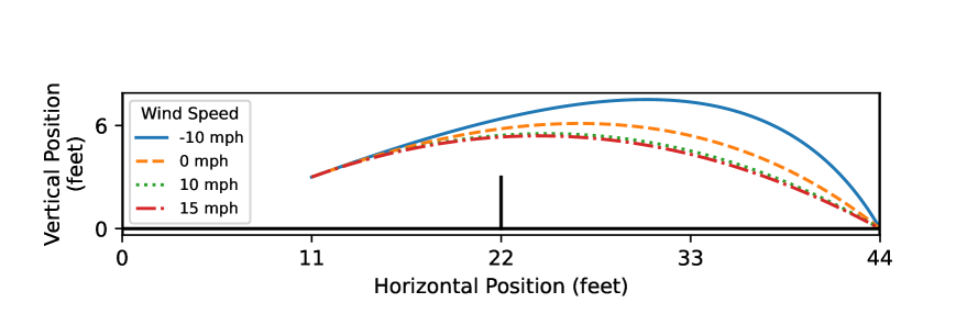
In Figure 2, we observe that the trajectories for wind speeds mph do not differ greatly. However, when playing against the wind (i.e. mph), the pickleball flight has greater curvature with a higher arc. It appears that the pickleball (which is light) gets held up by the wind. Towards the end of the path when playing against the wind, the pickleball is moving more in a downward vertical direction than horizontally.
4.2 Pickleball Velocity
We now consider an exercise with the same input values as given in Section 4.1. However, this time we calculate the velocity functions and . We evaluate the coordinate velocities and for increasing times . Then, the overall speed is calculated via . In Figure 3, we plot versus the horizontal location under the wind conditions mph, mph, mph and mph.
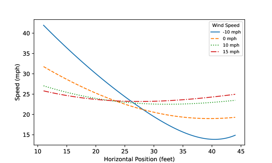
In Figure 3, we again observe that the condition of playing against wind (i.e. mph) is significantly different from the other three cases. For example, the initial velocity is greatest when playing against the wind. This is necessary in order for the shot to reach the right endline. When playing against the wind, we also observe greater initial deceleration (i.e. the slope of the velocity curve is steeper). On the other hand, when playing with the wind, the ball maintains a similar velocity throughout its path. Under all four wind conditions, we see that the pickleball speed is similar (approximately 24 mph) at the horizontal position 27 feet. The 27-foot position is close to the boundary of the non-volley zone (NVZ) on the right hand side of the court. From a playing perspective, this is interesting since the NVZ boundary is widely regarded as being the most strategic position.
4.3 Strategy - Playing in the Wind
Here we return to the primary strategic question: is it better to play with the wind or against the wind?
As mentioned at the beginning of Section 3.1, there are various shots in pickleball. Some shots are infrequent (e.g. lob shots). Smash shots are also less common than other shots, although it is apparent that a trailing wind makes smash shots even faster (i.e. more difficult to handle). Alternatively, some shots are not greatly affected by the wind. For example, dink shots are soft shots taken close to the net; consequently, they are not in the air for long periods of time. A case could be made that it is preferable to play against the wind when hitting the common drop shot. Against the wind, a player needs to worry less about “popping up” their drop shot and having it smashed back. The drop shot will be pushed down by the wind. Therefore, before endorsing playing against the wind over playing with the wind, we need to look at the common drive shot.
We now consider the merits of playing against the wind versus playing with the wind in the context of drive shots. For drive shots, we assume that the player of interest has played optimally in the sense that the ball is hit hard enough to bounce on the right endline should it be left untouched.
We use the general approach described in Section 3.1 to evaluate the time that it takes the ball to reach the opponent (i.e. point of interest in Figure 1). If it takes less time to reach the opponent playing with the wind, then playing with the wind is preferred. If it takes less time to reach the opponent playing against the wind, then playing against the wind is preferred. We calculate time differences under the following conditions: feet (corresponding to endline, mid-court and non-volley zone) for the player executing the shot, feet (corresponding to non-volley zone, mid-court and endline) for the opponent, launch angle degrees and launch height feet.
Letting denote the time in seconds that it takes the ball to reach the opponent with an assisting wind , we consider the excess time difference that it takes for the ball to reach the opponent when playing with the wind compared to when playing against the wind. This is evaluated for the wind conditions mph, mph and mph. Table 1 provides the results. We note that the time difference results in Table 1 are not greatly sensitive to minor modifications in the values of and .
| 0 | 29 | 0.097 | 0.200 | 0.346 |
|---|---|---|---|---|
| 0 | 33 | 0.056 | 0.166 | 0.348 |
| 0 | 44 | -0.302 | -0.490 | 0.089 |
| 11 | 29 | 0.082 | 0.150 | 0.242 |
| 11 | 33 | 0.058 | 0.133 | 0.255 |
| 11 | 44 | -0.230 | -0.375 | -0.568 |
| 15 | 29 | 0.075 | 0.131 | 0.203 |
| 15 | 33 | 0.059 | 0.124 | 0.223 |
| 15 | 44 | -0.203 | -0.332 | -0.505 |
From Table 1, we observe that most of the entries are positive. This suggests that there is a competitive advantage to playing against the wind when hitting the common drive shot. The ball reaches the opponent faster and there is less time for the opponent to react when playing against the wind. The only situations where is negative correspond to the setting feet (i.e. the opponent is located on the right endline). This is noteworthy since it is generally accepted pickleball strategy to approach the non-volley zone, and not sit back at the right endline.
It is also interesting to look at the row with input settings feet and feet. This corresponds to the common situation where both players have approached the non-volley zone and are as close as possible. Here, we see that as the wind increases, increases. That is, the advantage of playing against the wind becomes greater as the wind blows harder. In fact, this same phenomenon is observed in all situations in Table 1 whenever feet.
5 DISCUSSION
This paper appears to be the first serious investigation of flight dynamics in the sport of pickleball. Our main contribution is one of strategy; we argue that playing against wind is generally preferable to playing with the wind. Previously, there appeared to be no consensus opinion on the preference. The work is based on a detailed physical model that takes into account relevant inputs including air resistance and wind. Python code is provided in a github page (see the Appendix) that allows researchers to graph pickleball trajectories and velocities under various conditions.
Although the results provided in this paper correspond to our intuition and were derived from existing knowledge of projectile motion, it would be good to verify some of the results against video taken from pickleball matches. In future research, it may also be useful to consider additional wind environments such as crosswinds.
6 REFERENCES
- [1
-
] “2023 Sports, Fitness, and Leisure Activities Topline Participation Report”. Sports & Fitness Industry Association, 2024.
- [2
-
] Jim Albert, Mark E Glickman, Tim B Swartz, and Ruud Koning. “Handbook of statistical methods and analyses in sports”. CRc Press, 2017.
- [3
-
] Peter Chudinov. “Projectile motion in a medium with quadratic drag at constant horizontal wind”. 2022. arXiv: 2206.02397.
- [4
-
] John R Dormand and Peter J Prince. “A family of embedded Runge-Kutta formulae”. Journal of Computational and Applied Mathematics 6.1 (1980), pp. 19-26.
- [5
-
] Paramjit S Gill and Tim B Swartz. “A characterization of the degree of weak and strong links in doubles sports”. Journal of Quantitative Analysis in Sports 15.2 (2019), pp. 155-162.
- [6
-
] Marko V Lubarda and Vlado A Lubarda. “A review of the analysis of wind-influenced projectile motion in the presence of linear and nonlinear drag force”. Archive of Applied Mechanics (2022), pp. 1997-2017.
- [7
-
] Bruce R Munson, Donald F Young, and Theodore H Okiishi. “Fundamentals of Fluid Mechanics”. John Wiley & Sons Inc, 1997.
- [8
-
] Jenn Rossmann and Andrew Rau. “An experimental study of wiffle ball aerodynamics”. American Journal of Physics - AMER J PHYS (Dec. 2007). DOI: 10.1119/1.2787013.
- [9
-
] Pauli Virtanen et al. “SciPy 1.0: Fundamental Algorithms for Scientific Computing in Python”. Nature Methods 17 (2020), pp. 261-272. DOI: 10.1038/s41592-019-0686-2.
7 APPENDIX
This section provides details regarding the pickleball motion model. It is a projectile equation which takes into account the air resistance and wind speed. A similar model has been used in [3] to study the projectile motion in three other sports: badminton, tennis and golf. Before presenting the full mathematical equation, we introduce and recall previous notation related to the pickleball and its motion:
-
•
: mass
-
•
: flight time
-
•
: coordinates
-
•
: velocity
-
•
: speed
-
•
: initial speed
-
•
: initial launch angle
-
•
: horizontal constant wind speed.
The equation for projectile motion follows from Newton’s second law, where we only take into account the gravity and air resistance acting on the pickleball. The air resistance or the drag force is given by
| (5) |
where
-
•
is the density of the air,
-
•
is the cross-sectional area of the pickleball,
-
•
is the relative velocity of the pickleball with respect to the wind,
-
•
is the drag coefficient.
The drag coefficient varies with the Reynolds number
| (6) |
where is the pickleball speed relative to the air, is the diameter of the ball, is the air density, and is the dynamic viscosity of the atmosphere. The relation between and is in general a complicated nonlinear function that depends on the object shape, the object orientation, and characteristics of the air flow. Examples of for a smooth cylinder and a smooth sphere are shown in Figure 4, which was taken from Munson et al. [7].
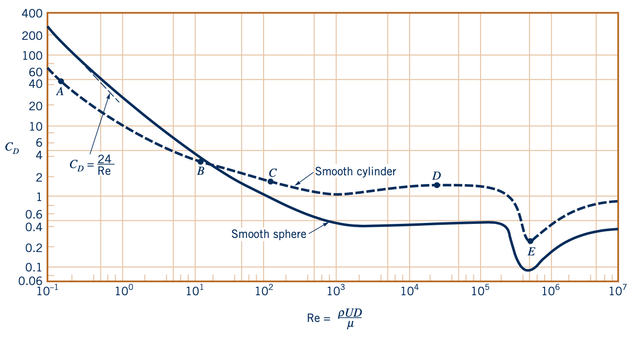
Though the functional form of can vary depending on the situation, it is roughly proportional to for low Reynolds numbers while turbulence, or irregular air motion, is minimal. At larger Reynolds numbers, when there is significant turbulence, evens out to stay roughly constant. As we can see from Fig. 4, the value for a smooth sphere stays on the same order of magnitude from a Reynolds number of about onward, though with a dip around before returning to its constant behaviour. Rougher surfaces tend to lower this threshold Reynolds number by increasing the turbulence around the sphere. Thus, we expect the holes in a pickleball to reduce the Reynolds number required to produce a roughly constant to a value even lower than .
The parameters in our problem correspond to , which is well above the threshhold of . Thus we conclude that should stay roughly constant. In terms of the exact value of this constant, since we could not find any experimental measurements of for pickleballs, we approximated the value by treating the pickleball as a forward-facing wiffleball and using the experimental results found by Rossmann et al. [8]. This gave us a constant of approximately 0.6 to use in Equation (5). The constant drag coefficient leads to a quadratic dependence of the drag force on the the relative velocity instead of a linear one as often used in projectile equations. The full system then has the form
| (7) | ||||
where is 0.6 as stated before, is the gravitational constant , is a standard atmospheric density of , is a standard cross-sectional area for a pickleball of , is a standard pickleball mass of g, denote the first order time derivatives which give the velocity and denote the second order time derivatives which give the acceleration of the ball.
System (7) is solved numerically using the explicit Runge-Kutta method of order 5(4) provided by default in Scipy’s [9] solve_ivp function [4]. The initial speed given implicitly by conditions in (3) are determined by using Scipy’s fsolve function to numerically solve for the roots of , using the functions we found. The Python code used to accomplish this is hosted at https://github.com/0Strategist0/Pickleball.
It should be noted that though our choice of is reasonable given the data we had and seems to produce pickleball trajectories and velocities similar to what is often measured, the true for a pickleball could in principle vary by roughly in certain conditions. We did test several such alternate values, and the exact numerical values for the time differences we obtained could be significantly different than the ones shown in this paper. However, the signs of all these time differences were preserved after varying , meaning that our main conclusions about whether to play with or against the wind seem to hold regardless of the specific value of . It would be interesting for future work to obtain experimental data measuring at a variety of Reynolds numbers, allowing for comparison with our model and the computation of more accurate numerical results.