z5261811@ad.unsw.edu.au, haowei.lou@student.unsw.edu.au, lina.yao@data61.csiro.au, yuzi20@lehigh.edu
-
August 2024
Brain Network Diffusion-Driven fMRI Connectivity Augmentation for Enhanced Autism Spectrum Disorder Diagnosis
Abstract
Functional magnetic resonance imaging (fMRI) is an emerging neuroimaging modality that is commonly modeled as networks of Regions of Interest (ROIs) and their connections, named functional connectivity, for understanding the brain functions and mental disorders. However, due to the high cost of fMRI data acquisition and labeling, the amount of fMRI data is usually small, which largely limits the performance of recognition models. With the rise of generative models, especially diffusion models, the ability to generate realistic samples close to the real data distribution has been widely used for data augmentations. In this work, we present a transformer-based latent diffusion model for functional connectivity generation and demonstrate the effectiveness of the diffusion model as an augmentation tool for fMRI functional connectivity. Furthermore, extended experiments are conducted to provide detailed analysis of the generation quality and interpretations for the learned feature pattern. Our code will be made public upon acceptance.
Keywords: fMRI, Latent Diffusion Models, Transformers, Autism Spectral Disorder, Data Augmentation, Generative Models
1 Introduction
Autism Spectrum Disorder (ASD) is a neurodevelopmental deficits that impacts how individuals communicate and interact with others (Lord et al., 2018). Common diagnostic practices include medical and neurological examinations, assessments of an individual’s cognitive and language abilities, and observation of behavior (Vahia, 2013, Lord et al., 2018). Among neurological examinations, Functional Magnetic Resonance Imaging (fMRI) has been widely adopted due to its ability to detect changes in blood flow within the brain, providing insights into the neural mechanisms underlying ASD (Ecker et al., 2015, Müller and Fishman, 2018). In practice, fMRI data is used to construct functional connectivity by analyzing blood-oxygen-level-dependent (BOLD) signals. These signals help examine functional correlations between Regions of Interest (ROIs) as defined by a brain atlas (Keown et al., 2013, Assaf et al., 2010, Hull et al., 2017, Han et al., 2024).
The advent of Machine Learning (ML) brings many ML-based diagnostic frameworks that can automatically diagnose a patient’s ASD status by analyzing functional connectivity (Haghighat et al., 2022, Wang et al., 2019, Sadeghian et al., 2021, Yan et al., 2019, Li, Zhou, Dvornek, Zhang, Gao, Zhuang, Scheinost, Staib, Ventola and Duncan, 2021, Kan et al., 2022). ML-based framework require lots of data to achieve good performance. However, collecting high-quality fMRI data necessitates professional operators, specialized equipment, and dedicated lab environments. This process is both expensive and resource-intensive. The problem of data scarcity limits the performance and generalizability of ML models for ASD diagnosis.
To address the problem of data scarcity, many researchers have tried data augmentation techniques to artificially expand the training dataset. For example, (Pei et al., 2022) proposed to add random Gaussian noise on functional connectivity and multiple functional connectivity construction with sliding window along ROI signals as data augmentation to improve the identification of Attention Deficit/Hyperactivity Disorder (ADHD) in fMRI studies. (Wang et al., 2022) used sliding windows of ROI signals as data augmentation technique to construct contrastive pairs for contrastive representation learning.
Building on these traditional methods, deep learning based approaches have pushed the frontier of data augmentation techniques. (Qiang et al., 2021) introduced RNN based Variational AutoEncoder (VAE) for ROI signals generation and augmentations to improve ADHD diagnosis. (Li, Wei, Chen and Schönlieb, 2021) used a GAN-based generator to generate functional connectivity for data augmentation of Alzheimer’s disease diagnosis. (Zhuang et al., 2019) proposed GAN and VAE combined framework that utilize 3-dimensional convolutions to generate high-dimensional brain image tensors for augmenting cognitive and behavioural prediction task. (Xia et al., 2021) provided an analysis of aging process and demonstrate the potential for data augmentation with conditional GAN. (Fang et al., 2024) developed an open-source software for fMRI data analysis and augmentation, covering BOLD signal augmentation and brain network augmentation. However, VAE & GAN are experiencing the problem of posterior collapse (Lucas et al., 2019) and mode collapse (Metz et al., 2016) respectively that can affect the generation quality.
Diffusion methods (Ho et al., 2020, Rombach et al., 2022), as a strong and competitive alternative generative model, have been applied to augment various types of medical images. These include micro-array images (Ye et al., 2023), skin images (Akrout et al., 2023), lung ultrasound images (Zhang et al., 2023), 3D brain MRI images (Pinaya et al., 2022), and chest X-Ray images exhibiting various abnormalities (Chambon et al., 2022, Packhäuser et al., 2023).
Despite these advancements, there is currently no diffusion-based data augmentation method specifically tailored for brain networks in the form of functional connectivity. Adapting diffusion models to generate functional connectivity faces several challenges. First, the non-Euclidean nature of functional connectivity does not meet the prerequisites of convolutional neural networks (CNNs), making standard diffusion models, which are typically designed for image generation, unsuitable. Second, the numeric distribution of functional connectivity does not conform to the standard Gaussian distribution. As such, the mismatch between the signal and noise distributions, where classic diffusion models use standard Gaussian noise, challenges the assumption that input signals and noise follow the same distribution (Ho et al., 2020). Finally, the small data size and complexity of functional connectivity patterns make it difficult for the diffusion model to effectively learn condition-specific features, rendering conditioning mechanisms like adaptive layer normalization ineffective.
In this work, we proposed Brain-Net-Diffusion, a pure transformer-based latent diffusion model for fMRI data generation and augmentation in the form of functional connectivity. Developed based on Diffusion Transformer (Peebles and Xie, 2023), our Brain-Net-Diffusion has three key designs which make it more suitable for functional connectivity generation. Firstly, Brain-Net-Diffusion uses transformers for both latent ROI feature encoding and diffusion denoising. The attention mechanism allows modeling interactions between ROIs all at once. Furthermore, to resolve the problem of distribution gap between encoded latent space and scheduled noise in diffusion process, Brain-Net-Diffusion uses distribution normalization module to ensure the generated connectivity follows the same numerical distribution with the real connectivity. Finally, to tackle the problem of ineffective conditioning during diffusion process, Brain-Net-Diffusion uses an extra constraint on conditional embedding to ensure the effectiveness of conditioning.
Our contributions can be summarized as following:
-
•
We proposed Brain-Net-Diffusion, a transformer-based latent diffusion model specifically designed for functional connectivity modeling and generation.
-
•
We introduced an distribution normalization module to tackle the problems of distribution gap between encoded latent space and scheduled noise.
-
•
We introduced conditional contrastive loss to address the problem of ineffective conditioning mechanism for adapting diffusion transformer to resting state fMRI functional connectivity.
-
•
We conduct extensive experiments to assess the quality of the generated data and demonstrate that our data augmentation method can effectively improve ML model performance, outperforming 3% of existing state-of-the-art methods.
2 Brain Network Diffusion Model
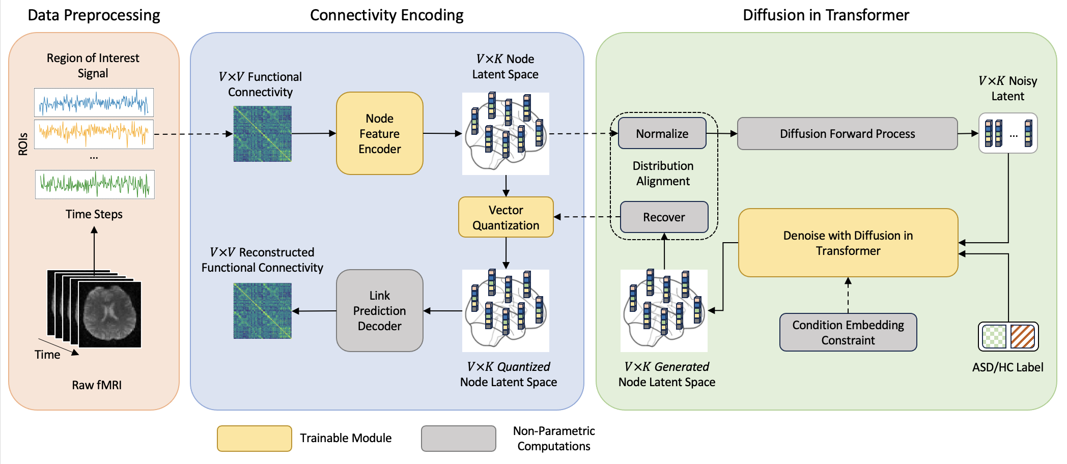
Brain-Net-Diffusion is a diffusion-based generative model designed to generate in-distribution and diverse functional connectivity matrices. These generated matrices are intended to address the issue of data scarcity and enhance the performance of downstream ASD classification models. Figure 1 provides an overview of the Brain-Net-Diffusion model. The model is composed of the following three main modules.
Latent Connectivity Auto-Encoder, which encodes functional connectivity into a latent space that contains representations for each ROI. Conditional Diffusion Transformer which generates new latent representations using diffusion model. Functional Connectivity Generator which integrates the Latent ROI Auto-Encoder and Conditional Diffusion Transformer to generate new functional connectivity matrices.
Latent Connectivity Auto-Encoder and Conditional Diffusion Transformer are trained separately, each with distinct loss functions. Further details on these modules and training objectives will be provided in the following sections.
2.1 Latent Connectivity Auto-Encoder
We deployed a Vector Quantized-Variational Autoencoder (VQ-VAE) as the Latent Connectivity Auto-Encoder to efficiently encode and discretize functional connectivity matrices into a structured latent space.
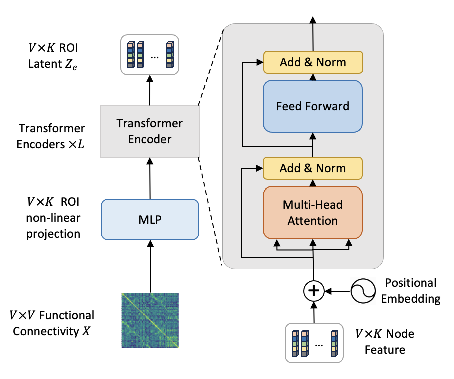
Figure 2 illustrates the architecture of the VQ-VAE, which consists of three key components: (1) Encoder that maps the functional connectivity matrix to a latent representation , where is the number of ROIs and is the latent feature dimension for each ROI; (2) Vector Quantization (VQ, (Van Den Oord et al., 2017)), which converts into a quantized latent representation ; and a (3) Decoder, that reconstructs the functional connectivity matrix from .
2.1.1 Latent Encoder
Given a functional connectivity matrix , where each row of represents the correlation of each ROI with all other ROIs, we projected to a -dimensional feature space using a linear transformation followed by a ReLU activation function. This process produced transformed ROI features , where each row represents the transformed feature of an ROI. We then passed through layers of a Transformer encoder (Vaswani et al., 2017), where each ROI’s transformed feature served as a token. We leveraged the capability of multi-head self-attention to dynamically weigh the importance of each ROI during the encoding process, producing latent features . More details on the encoding process can be found in Figure 2(a).
2.1.2 Vector Quantization
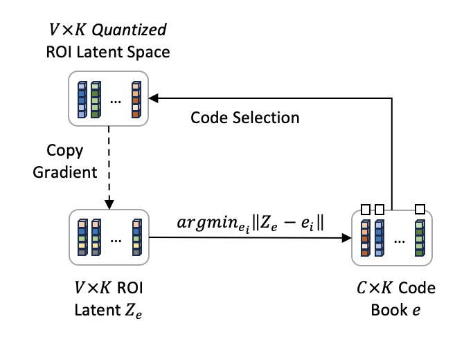
Following the approach of the latent diffusion model (Rombach et al., 2022), we used VQ to discretize the latent features and address issues such as ”posterior collapse” (Van Den Oord et al., 2017).
A codebook is initialized with a set of learnable representation vectors, where is the size of the codebook, and is the dimensionality of the codebook vectors. For each latent feature vector in the latent space , the corresponding quantized latent feature is determined by finding the nearest neighbor in the codebook, as shown in Equation 1.
| (1) |
During training, the codebook vectors are iteratively updated to minimize the reconstruction loss. This is achieved by adjusting the codebook vectors to be closer to the input vectors assigned to them, typically using the loss to measure the difference. The VQ operation is illustrated in Figure 2(b).
2.1.3 Functional Connectivity Decoder
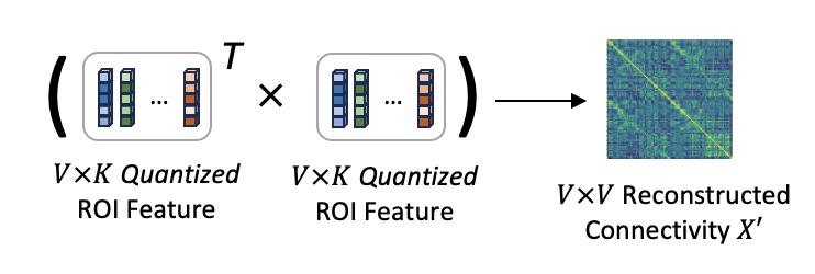
To reconstruct the functional connectivity from the quantized latent features , we adapted the matrix multiplication decoding approach used in link prediction tasks (Kipf and Welling, 2016, Salha et al., 2019) as our decoder. The output functional connectivity matrix is reconstructed by computing the dot product () of the quantized latent features, i.e., , .
2.1.4 Training Objective
Followed (Van Den Oord et al., 2017), we combined VQ, reconstruction and commitment loss to train our Latent Connectivity Auto-Encoder, as shown in Equation 2:
| (2) |
where denotes the latent features produced by the encoder, refers to the codebook containing learnable vectors, is the original functional connectivity matrix, and represents the quantized latent features derived from the codebook, and the operator is the stop-gradient operator, which prevents gradients from flowing through its argument during backpropagation.
The VQ loss adjust the codebook vectors towards the encoder outputs , the reconstruction loss is used to optimize the encoder, ensuring that the reconstructed matrix closely resembles the original functional connectivity matrix , and the commitment loss is employed to encourage the encoder outputs to map to the nearest feature in the codebook.
2.2 Conditional Diffusion Transformer
Once the latent Connectivity Auto-Encoder is trained, it allows us to encode functional connectivity into latent representations . We transformed it into a Gaussian distribution by applying z-score normalization to . We then train a diffusion model over , with the model conditioned on the subject’s status (such as ASD or HC).
2.2.1 Forward Diffusion Process
The forward diffusion process gradually adds noise to at each timestep . This process is mathematically described by the following transition distribution:
| (3) |
where represents a normal distribution, is a time-dependent scaling factor, and is identity matrix. The parameters control the amount of added noise in the process.
To facilitate the generation of at a specific timestep , we reparameterize the process as:
| (4) |
where is sampled from a standard normal distribution .
2.2.2 Reverse Diffusion Process
The reverse diffusion process is designed to systematically denoise and recover the original , which corresponds to the normalized latent feature . This process is modelled as a series of conditional distributions, where the transition from to at each timestep is given by:
| (5) |
where denotes a normal distribution, with the mean and covariance predicted by a transformer-based noise prediction network, which is parameterized by the learnable parameters .
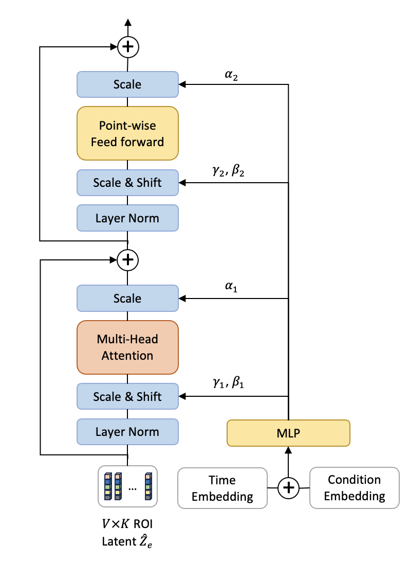
We used the same architecture as the Diffusion Transformer (Peebles and Xie, 2023) for our noise prediction network in the reverse diffusion process, as shown in Figure 4. It consists of a series of transformer blocks that predict the noise present in . To effectively incorporate conditioning information, we use adaptive layer normalization (adaLN), where the normalization parameters are dynamically adjusted based on the conditioning input:
| (6) |
Here, and are learned functions that depend on the conditioning variables (time step) and (class label).
2.2.3 Training Objective
The original diffusion transformer noise predictor is trained by minimizing the L2 loss between the predicted noise and the true noise :
| (7) |
where (which equals ) is the initial normalized latent feature, is the noisy latent feature at timestep , is the Gaussian noise, and is the noise prediction network predicted noise at timestep .
To enhance the distinctiveness of class embedding and ensure the effectiveness of both time and condition embedding, we introduced condition contrastive loss, which contains two additional loss terms:
Maximizing the distances between each label embedding: We start with an embedding table , where is the number of classes, and is the dimension of each embedding. The pairwise distance matrix captures the distances between every pair of embedding and using the Euclidean distance:
| (8) |
To ensure that each class has a distinct embedding, the first loss term focuses on maximizing the distances between different class embedding (excluding the distance of an embedding to itself):
| (9) |
Balancing time and condition embedding: To make sure both time and condition embedding are equally effective, we introduce a second loss term. This term minimizes the difference in mean of element-wise absolute value between the time embedding and the condition embedding:
| (10) |
where is the time embedding, is the condition embedding and is the dimension for both embedding.
The overall loss for the noise prediction network combines the original noise prediction loss with these additional terms:
| (11) |
where minimize the sampled and predicted loss, maximizes the pairwise distances between class embedding, and balances the numerical scales of the embedding.
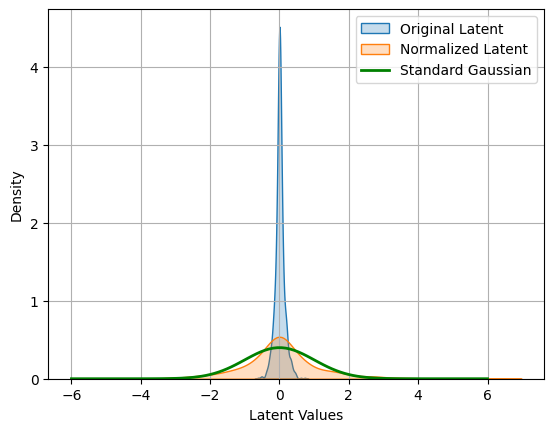
2.2.4 Distribution Normalization
We introduced the distribution normalization module to address the numerical distribution gap between the scheduled noise in the diffusion process and the encoded ROI latent features. The distribution normalization module normalizes the ROI features to a standard Gaussian distribution with Z-score normalization before the diffusion training and generation processes. The encoded latent representation is first normalized to , which is then used during the diffusion process.
After the reverse diffusion process generates the new ROI latent representation , it is de-normalized to the original latent space, transforming it into . This ensures that matches the distribution of the original encoded latent feature .
Specifically, for each data batch that was inputed into the forward diffusion process, we applied z-score normalization to the latent distribution:
| (12) |
where is the batch mean and is the batch standard deviation. The diffusion transformer was trained on and generated within the normalized latent space . During the generation process, we compute the batch mean and standard deviation of the original latent features, then de-normalize the generated latent features back to the original latent space using the reverse of Equation 12. The distribution comparison of the original and normalized latent spaces is shown in Figure 3.
2.3 Functional Connectivity Generator
The trained VQ-VAE (Sec. 2.1) and the Conditional Diffusion Transformer (Sec. 2.2) are deployed together for new connectivity generation. The generation process begins with an initial noise sample and a dsired condition for the generated sample. This noisy representation is then processed by the reverse diffusion process with the trained noise predition network . At each step, the model predicts and removes the noise:
| (13) |
iteratively refining over steps until the noise is fully removed. It produces a latent feature that accurately reflects the desired condition.
Next, is de-normalized using the reverse Z-score function to ensure it matches the distribution of the latent feature produced by the VQ-VAE encoder. Finally, the de-normalized latent feature is discretized using the VQ (Sec.2.1.2) and passed through the decoder (Sec.2.1.3) to produce the final functional connectivity matrix tasks for downstream ASD classification tasks.
2.3.1 Real Sample Guidance
While the standard reverse diffusion process typically starts from pure Gaussian noise, this approach can sometimes result in out-of-distribution samples. To mitigate this and improve the generation quality, we incorporated ROI features encoded from real connectivity as guidance during the generation process. Inspired by prior work on data augmentation for images (Trabucco et al., 2023, Meng et al., 2021), we spliced an encoded ROI feature from a real connectivity matrix into the diffusion process.
Given a reverse diffusion process with steps, we inserted an encoded latent from the real connectivity matrix with added noise at a specific timestep , where guidance level is a hyperparameter controlling the insertion position:
| (14) | ||||
| (15) |
The reverse diffusion process then continues from this spliced latent at timestep until the final sample is generated. As , the generated connectivity are more closely resemble the guidiance connectivity.
2.3.2 Condition Contrastive Augmentation
For the generation condition in the reverse diffusion process, with guidance from real samples, can either match or oppose the condition of the guide real connectivity. We performed generation with both conditions for each guidance real connectivity, to improve the diversity of the generated dataset.
Specifically, we constructed the generated dataset from the original dataset
| (16) |
where is the real functional connectivity for one subject, and is the condition (ASD or HC) of the subject.
The generated dataset for augmentation is the union of guidance identical condition set and guidance opposite condition set . The connectivity in is generated with condition identical to the guidance real connectivity:
| (17) |
where stands for the trained Brain-Net-Diffusion connectivity generator, denotes the guidance level and denotes the condition (ASD or HC) of the guidance real connectivity . Conversely, consists of connectivity generated under conditions that are opposite to those used in the guidance real connectivity:
| (18) |
The motivation for condition contrastive augmentation with the union of identical and opposite condition-generated data is to maximize the knowledge learned from the conditional latent diffusion and improve the diversity of the generated dataset.
2.4 Overall Pipeline
Algorithm 1 provides the pseudo code for Brain-Net-Diffusion training process. It includes training for Latent Connectivity Auto-Encoder and Conditional Diffusion Transformer.
Algorithm 2 describes the connectivity generation module for Brain-Net-Diffusion. It integrates the trained connectivity auto-encoder and conditional diffusion transformer to generate new connectivity.
Algorithm 3 describes how the augmentation dataset is generated with real sample guidance and condition contrastive augmentation.
3 Experiment Settings
3.1 Dataset and Preprocessing
We collected rs-fMRI data from 505 ASD and 530 healthy control (HC) subjects from the Autism Brain Imaging Data Exchange I (ABIDE-I) dataset (Di Martino et al., 2014), which includes data from 17 international sites. This dataset was used to evaluate the performance of our method. Given a series of fMRI readings in with length , we used the Configurable Pipeline for the Analysis of Connectomes (Li, Esper, Ai, Giavasis, Jin, Feczko, Xu, Clucas, Franco, Heinsfeld et al., 2021) to preprocess the fMRI data. The CC200 atlas (Craddock et al., 2012) was used to segment the fMRI data into ROI signals , where is the number of ROIs.
The functional connectivity for each subject was constructed by computing the Pearson correlation between all pairs of ROI signals along the time dimension. Formally,
| (19) |
where is the functional connectivity matrix, and and are the signals of the th and th ROI, respectively.
We performed a stratified 5-fold cross-validation based on testing site and diagnosis labels to evaluate the performance of our method. In each fold, 60% of data was used for training, 20% for validation, and 20% for testing.
3.2 Implementation Details
Brain-Net-Diffusion was implemented using PyTorch and trained on a Linux system equipped with an NVIDIA RTX A5000 GPU (24GB VRAM) and 256GB of RAM.
The Latent Connectivity Auto-Encoder consists of a linear projection layer followed by four transformer blocks. We set code book size and codebook vector dimension . We trained for a maximum of 800 epochs with a batch size of 64, with an average training time of 50 minutes per fold.
The Conditional Diffusion Transformer has 14 DiT blocks and generates a latent vector with a dimension of 128. We set the number of diffusion steps to 100 and the dimension of time embedding, condition embedding and latent features are all set to 64. We trained for a maximum of 600 epochs with a batch size of 64, with an average training time of 2 hours per fold.
3.3 Augmentation Settings
We used the Brain-Net-Diffusion with real sample guidance to augment the training set. We combined dataset generated with Condition Contrastive Augmentation (Sec. 2.3.2), at guidance level (Sec. 2.3.1), to construct the generated dataset for augmentation.
We adopt a balanced data sampling strategy similar to the approach in (Trabucco et al., 2023) to train the downstream ASD classification model. This strategy ensures each training batch consists of an equal split, with half of the connectivity matrices drawn from the real connectivity set and the other half from the generated connectivity set
We employed a simple MLP classifier with 100-dimensional hidden layer followed by a ReLU activation function and a readout layer to perform downstream ASD classification. The classifier input is the flattened lower triangular portion of the functional connectivity matrix, sized at . The MLP was trained with a batch size of 256 and a dropout rate of 0.2.
We compared the downstream ASD versus HC classification performance of our methods with two classical augmentation and two generative approaches:
1) Gaussian Noise (Pei et al., 2022): This approach generates new samples by adding Gaussian noise to the original connectivity matrix. It aims to reduce the learning of useless high-frequency features and improve the model robustness. For each connectivity matrix, we sampled Gaussian noises with and and added the noise matrix to the original connectivty matrix separately to generate new samples.
2) Sliding Windows (Pei et al., 2022): The sliding window correlation method studies dynamic functional connectivity by continuously sliding and computing pairwise ROI correlations within a window. We adapted the non-overlapping sliding methods, where each ROI signal is equally split into non-overlap segments along time series and pairwise correlation is computed for each segments.
3) DRVAE (Qiang et al., 2021): DRVAE combines a VAE with a recurrent neural network to perform data augmentation for time-series data. While the original work is a generative model for ROI signal, we use its generated signal to compute functional connectivity for downstream classification models.
4) VAE-GAN (Qiang et al., 2023): This method combines VAE and GAN to leverage the strengths and mitigate the weaknesses of both models. VAE-GAN collapses the decoder and the generator into one model. We used the generated fMRI time-series data to compute functional connectivity for downstream models.
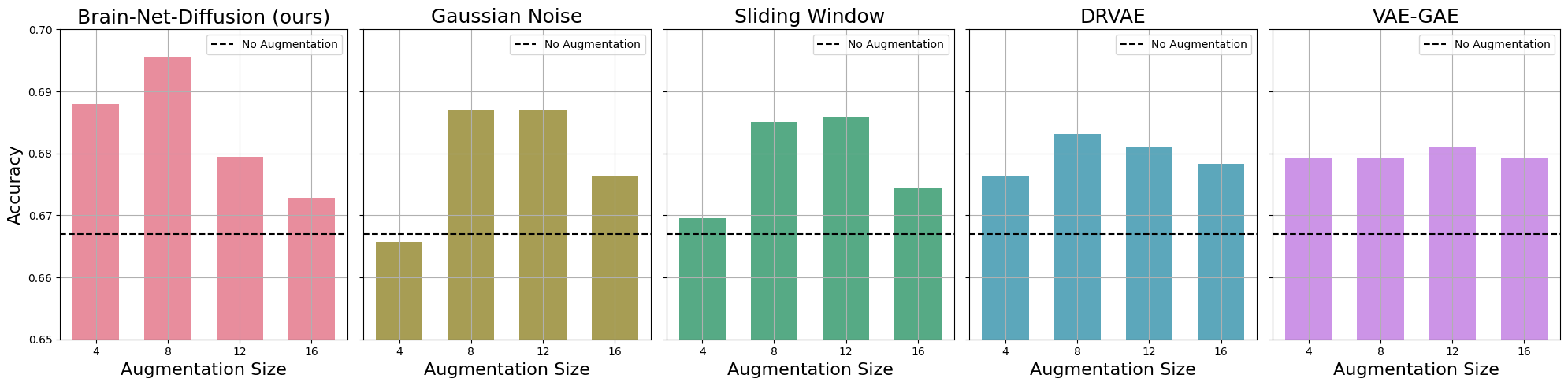
To ensure a fair and comprehensive comparison, we took account for different augmentation size for each methods. For each original sample, we tested different generated data sizes of 4, 8, 12, 16 for each augmentation method.
4 Results and Discussion
4.1 Overall Performance
Figure 5 illustrates the classification accuracy comparison across different augmentation methods, varying by the number of augmented samples. Our Brain-Net-Diffusion achieved the highest accuracy at 0.696 with an augmentation size of eight. We observed that both excessively large and very small augmentation sizes did not lead to optimal performance. One possible explanation is that too many generated samples can reduce the overall quality of the dataset, and too few samples do not add enough variety to enhance the augmentation effectively.
Table 1 reports the ASD classification performance on the test set, comparing performance with and without various augmentation methods. Augmentation using Brain-Net-Diffusion increased accuracy by 4.3% compared to no augmentation. It also outperformed other augmentation methods by margins ranging from 1.3% to 2.2% in accuracy.
| Augmentation | AUROC | Accuracy | Sensitivity | Specificity |
|---|---|---|---|---|
| No Augmentation | 0.738 0.030 | 0.667 0.029 | 0.660 0.104 | 0.674 0.067 |
| DRVAE | 0.754 0.012 | 0.683 0.006 | 0.697 0.044 | 0.670 0.048 |
| Gaussian Noise | 0.753 0.012 | 0.687 0.014 | 0.713 0.024 | 0.659 0.035 |
| Sliding Window | 0.763 0.026 | 0.686 0.027 | 0.714 0.042 | 0.658 0.056 |
| VAE-GAN | 0.755 0.012 | 0.681 0.012 | 0.698 0.060 | 0.664 0.048 |
| BrainNetDiffusion (ours) | 0.765 0.021 | 0.696 0.012 | 0.730 0.042 | 0.660 0.039 |
4.2 Impact of Distribution Normalization and Condition Contrastive Loss
To validate the effectiveness of our designed modification based on diffusion transformer - distribution normalization and condition contrastive loss, we tested the downstream ASD classification performance with the generated sample from the Brain-Net-Diffusion without each components, respectively. For each real connectivity with guidance level , we generate two ASD and two HC connectivity matrices, resulting in a total of eight generated samples per real sample.
Table 2 reports the ASD classification performance on the test set following the removal of Distribution Normalization and Condition Contrastive Loss from our Brain-Net-Diffusion model. The removal of Condition Contrastive Loss alone led to a 2.8% decrease in accuracy, while the removal of Distribution Normalization resulted in a 3.8% decrease. When both components were removed simultaneously, accuracy decreased substantially by 9.7%. This underscores the significant impact of both modules on the augmentation performance of Brain-Net-Diffusion.
4.3 Impact of Real Sample Guidance
To validate the necessity of Real Sample Guidance during the generation process (2.3.1), we tested the downstream ASD classification performance with the augmented dataset generated by Brain-Net-Diffusion without any guidance and with different guidance rates. We constructed three augmentation set: (1) 4 ASD and 4 HC connectivity with guidance level (no guidance), (2) 2 ASD and 2 HC connectivity with guidance level and (3) 2 ASD and 2 HC connectivity with guidance level .
Table 3 illustrates ASD classification performance on the test set with augmented connectivity generated at various guidance levels. Optimal results were achieved with smaller guidance levels of . This is expected as generation without guidance may produce low-quality connectivity, and generation with excessive guidance may reduce diversity, rendering the guidance less effective.
| DN | CCL | AUROC | Accuracy | Sensitivity | Specificity |
|---|---|---|---|---|---|
| 0.711 0.014 | 0.628 0.082 | 0.524 0.297 | 0.739 0.154 | ||
| ✓ | 0.736 0.015 | 0.669 0.024 | 0.714 0.075 | 0.622 0.056 | |
| ✓ | 0.755 0.028 | 0.676 0.025 | 0.687 0.048 | 0.665 0.061 | |
| ✓ | ✓ | 0.765 0.021 | 0.696 0.012 | 0.730 0.042 | 0.660 0.039 |
| Guidance Level | AUROC | Accuracy | Sensitivity | Specificity |
|---|---|---|---|---|
| No Guidance | 0.752 0.020 | 0.678 0.021 | 0.698 0.047 | 0.658 0.030 |
| 0.765 0.021 | 0.696 0.012 | 0.730 0.042 | 0.660 0.039 | |
| 0.742 0.023 | 0.673 0.031 | 0.694 0.010 | 0.652 0.056 |
| Condition Set | AUROC | Accuracy | Sensitivity | Specificity |
|---|---|---|---|---|
| (identical) | 0.752 0.016 | 0.683 0.017 | 0.719 0.039 | 0.646 0.051 |
| (opposite) | 0.725 0.037 | 0.664 0.038 | 0.707 0.062 | 0.618 0.030 |
| 0.765 0.021 | 0.696 0.012 | 0.730 0.042 | 0.660 0.039 |
4.4 Impact of Condition Contrastive Augmentation
To validate the necessity of Condition Contrastive Augmentation (2.3.2), we compared the downstream ASD classification performance with (1) the identical condition generated set only, (2) the opposite condition generated set only and (3) the union of (1) and (2). For this experiment, we fixed . For the identical and opposite generated set, we generated four connectivity for each corresponding real guidance. For the union, we generated two connectivity for each condition for each corresponding real guidance. Thus, augmentation size for each real connectivity is fixed at eight for all generated set in this experiment.
Table 4 shows the ASD classification performance on the test set with augmentation consisting of identical, opposite, and union conditional generations. In terms of AUROC and accuracy, augmentation using identical conditions proved less effective than the other two approaches. The union of identical and opposite condition augmentation achieved optimal performance, demonstrating the benefit of diversified training conditions in enhancing model robustness and generalization.
4.5 Evaluation for Generated Connectivity
We used qualitative and quantitative evaluation methods to interpret the generated functional connectivity matrices and evaluate their impacts on improving the performance of the downstream ASD classification model.
4.5.1 Quantitative Evaluation
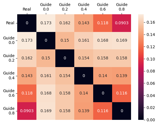
We computed the average pairwise MAE to quantify the differences between the real and generated functional connectivity matrices. Specifically, each entry in the average pairwise MAE is defined by
| (20) |
where is the dataset of all subjects’ connectivity, is real connectivity and is the corresponding generated connectivity matrix, guided by at different guidance levels. We generate one connectivity for each real connectivity at each guidance level of 0.0, 0.2, 0.4, 0.6 and 0.8.
Figure 6 illustrates the pairwise Mean Absolute Error (MAE) between real and generated connectivity. The results reveal three key observations. First, the pairwise MAE for train and test generation results are similar, indicating that Brain-Net-Diffusion demonstrates strong generalization capabilities. Second, the MAE between real and generated connectivity decreases as the guidance level increases, aligning with the expectation that higher guidance levels produce connectivity that more closely resembles the real data. Lastly, the MAE between generated connectivity and connectivity generated at different guidance levels is inversely proportional to the target connectivity guidance level. Specifically, connectivity generated with a lower guidance level exhibits a larger MAE when compared to connectivity generated with a higher guidance level.

4.5.2 Qualitative Evaluation
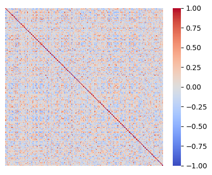
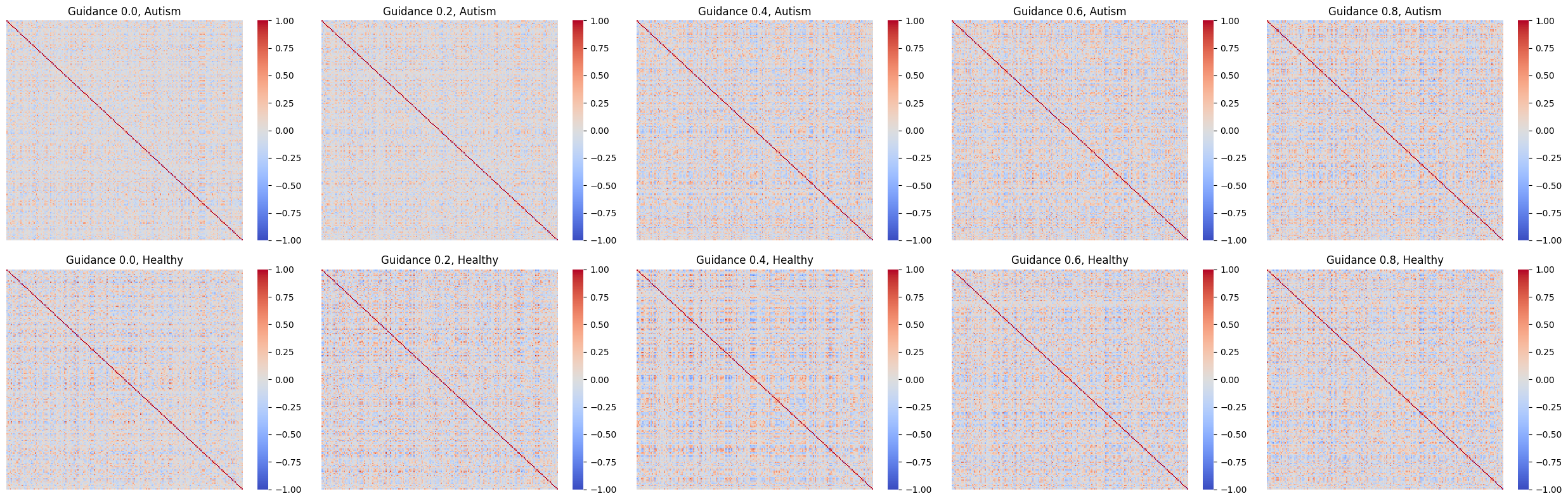
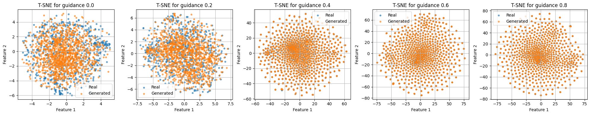
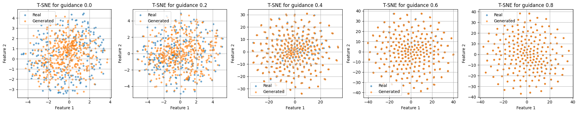
We visualized the real and generated functional connectivity matrices to qualitatively evaluate the structure and realism of the generated matrices. First, we draw the adjacency matrix of both real and generated connectivity to visually compare their structures. Next, we flattened the adjacency matrices and applied T-SNE dimensionality reduction (Van der Maaten and Hinton, 2008) to project the high-dimensional connectivity into a lower-dimensional space. It allowed us to observe clustering patterns and assess how well the generated matrices align with the real connectivity. We generated one ASD and one HC functional connectivity with guidance level 0.2, 0.4, 0.6 and 0.8 for samples in both train and test set.
Figure 7 presents a real functional connectivity alongside its generated counterparts produced by Brain-Net-Diffusion at varying guidance levels and conditions. The results show that the generated connectivity networks are visually similar to the real ones. This visual similarity provides a preliminary indication that Brain-Net-Diffusion is capable of generating functional connectivity that closely resembles real data.
Figure 8 presents the T-SNE visualization of real and generated functional connectivity, of training and testing set, respectively. The results show that the generated connectivity follows a similar distribution with the real connectivity, and the similarity increases as the guidance level increases.
4.6 Biomarker Interpretations
We designed and validated a sampling and distance computation algorithm to identify the important ROIs for ASD classification, based on our trained Brain-Net-Diffusion. Furthermore, by mapping the ROIs to the Yeo 7 Networks (Yeo et al., 2011), we provided a function module-level analysis for ASD brain dysfunction.
4.6.1 ROI importance computation
To analysis the importance of each ROI for ASD classifications, we leveraged the trained noise predictor within the Conditional Diffusion Transformer (Sec. 2.2.2). Starting from the same initial Gaussian noise, the noise predictor generates different predicted noise for each ROI under different conditions (ASD and HC). This variation arises due to adaptive layer normalization (Equation 6), which scales and shifts the features of each ROI according to the given condition. By measuring the differences in predicted noise between the two conditions for each ROI, we assess the sensitivity of each ROI to the condition change. The greater the difference, the more sensitive the ROI is, indicating its potential importance in classification.
Algoithm 4 presents the ROI importance score calculation method. It first samples Gaussian noise and generates predicted noise for both conditions (ASD and HC) using the noise predictor . For each ROI, we calculated the Euclidean distance between the predicted noise under the two conditions. These distances are averaged over multiple noise samples to produce a final importance score for each ROI, where higher scores indicate greater sensitivity and thus higher importance for classification.
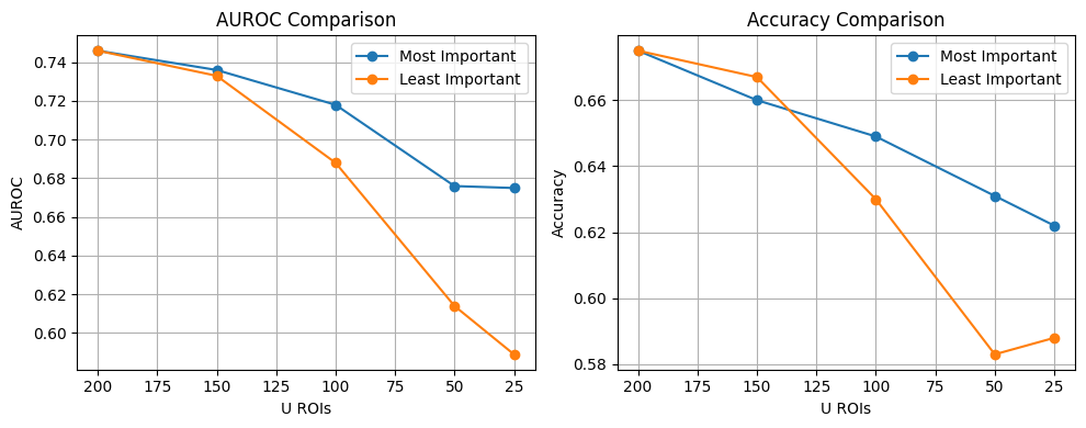
4.6.2 Importance Score Validation
To validate the importance of ROIs interpreted from the Brain-Net-Diffusion, we compared the ASD classification performance on the functional connectivity of the most important ROIs versus the least important ROIs. The hypothesis is that if ROIs are correctly ranked by their importance, as defined by Brain-Net-Diffusion, then the most important ROIs should capture more ASD-relevant features, leading to better classification performance compared to the least important ROIs.
We started with the original functional connectivity matrix and constructed a new connectivity matrix of shape using the rows and columns corresponding to the selected ROIs. An MLP classifier with 100 hidden units was trained using the flattened lower triangular part of this cropped connectivity matrix as input.
Figure 9(a) reports the MLP classification performance on the connectivity of the top- most important and the bottom- least important ROIs, . The results reveal that while classification performance declines for both sets of ROIs as decreases, the ROIs identified as important by the diffusion model consistently outperform those deemed least important. This supports the accuracy of the importance scores assigned to the ROIs by the diffusion model.
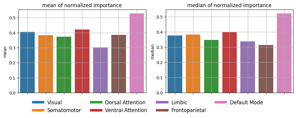
4.6.3 Functional Module Analysis
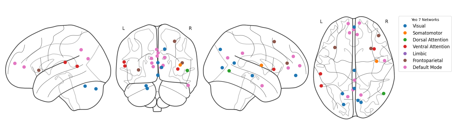
We provided a functional module-level analysis by mapping the ROIs and their importance scores to Yeo 7 networks (Yeo et al., 2011). Yeo 7 networks divide the brain into seven distinct functional networks based on resting-state fMRI, including Visual, Somatomotor, Dorsal Attention, Ventral Attention, Limbic, Frontoparietal and Default Mode.
Figure 9 shows the center of mass of the 25 most important ROIs interpreted by our diffusion transformer, along with their respective networks. These ASD-relevant ROIs are distributed across various brain regions, with 7 ROIs belonging to the Visual network and 10 ROIs to the Default Mode network.
We calculated the average and median importance scores for the ROIs mapped into each network as a measurement to evaluate which network is most important for ASD classification,. Figure 9(b) illustrates these scores for all 7 networks. The Default Mode network shows the highest mean and median importance scores. In contrast, the Limbic network has the lowest mean importance score, and the Frontoparietal network exhibits the lowest median importance score.
These results suggest that the Default Mode network is most strongly related to ASD classification. This aligns with behavioral observations from fMRI studies and supports the prevailing theory that ASD involves alterations in cognitive networks while preserving or altering sensory processing areas(Robertson et al., 2013, Turkeltaub et al., 2004, Iuculano et al., 2014).
5 Conclusion
In conclusion, we propose Brain-Net-Diffusion to address the issue of data scarcity in fMRI-based ASD classification. By augmenting the training data using the Brain-Net-Diffusion model, the downstream ASD classification model can leverage a richer dataset to improve accuracy in identifying ASD. Additionally, we introduce two new modules in the training and generation process: distribution normalization and conditional contrastive loss, which contribute to a more sophisticated training approach. We conducted extensive experiments and analysis. Our results indicate that our proposed data augmentation model can significantly enhance the performance of ASD classification model. Future research could explore the application of Brain-Net-Diffusion to other neurodevelopmental disorders and investigate its potential integration with other advanced machine learning techniques.
References
- (1)
- Akrout et al. (2023) Akrout M, Gyepesi B, Holló P, Poór A, Kincső B, Solis S, Cirone K, Kawahara J, Slade D, Abid L et al. 2023 in ‘International Conference on Medical Image Computing and Computer-Assisted Intervention’ Springer pp. 99–109.
- Assaf et al. (2010) Assaf M, Jagannathan K, Calhoun V D, Miller L, Stevens M C, Sahl R, O’Boyle J G, Schultz R T and Pearlson G D 2010 Neuroimage 53(1), 247–256.
- Chambon et al. (2022) Chambon P, Bluethgen C, Langlotz C P and Chaudhari A 2022 arXiv preprint arXiv:2210.04133 .
- Craddock et al. (2012) Craddock R C, James G A, Holtzheimer III P E, Hu X P and Mayberg H S 2012 Human brain mapping 33(8), 1914–1928.
- Di Martino et al. (2014) Di Martino A, Yan C G, Li Q, Denio E, Castellanos F X, Alaerts K, Anderson J S, Assaf M, Bookheimer S Y, Dapretto M et al. 2014 Molecular psychiatry 19(6), 659–667.
- Ecker et al. (2015) Ecker C, Bookheimer S Y and Murphy D G 2015 The Lancet Neurology 14(11), 1121–1134.
- Fang et al. (2024) Fang Y, Zhang J, Wang L, Wang Q and Liu M 2024 arXiv preprint arXiv:2405.06178 .
- Haghighat et al. (2022) Haghighat H, Mirzarezaee M, Araabi B N and Khadem A 2022 Journal of Neural Engineering 19(5), 056034.
- Han et al. (2024) Han S, Sun Z, Zhao K, Duan F, Caiafa C F, Zhang Y and Solé-Casals J 2024 Journal of Neural Engineering 21(1), 016013.
- Ho et al. (2020) Ho J, Jain A and Abbeel P 2020 Advances in neural information processing systems 33, 6840–6851.
- Hull et al. (2017) Hull J V, Dokovna L B, Jacokes Z J, Torgerson C M, Irimia A and Van Horn J D 2017 Frontiers in psychiatry 7, 205.
- Iuculano et al. (2014) Iuculano T, Rosenberg-Lee M, Supekar K, Lynch C J, Khouzam A, Phillips J, Uddin L Q and Menon V 2014 Biological psychiatry 75(3), 223–230.
- Kan et al. (2022) Kan X, Dai W, Cui H, Zhang Z, Guo Y and Yang C 2022 Advances in Neural Information Processing Systems 35, 25586–25599.
- Keown et al. (2013) Keown C L, Shih P, Nair A, Peterson N, Mulvey M E and Müller R A 2013 Cell reports 5(3), 567–572.
- Kipf and Welling (2016) Kipf T N and Welling M 2016 arXiv preprint arXiv:1611.07308 .
- Li, Wei, Chen and Schönlieb (2021) Li C, Wei Y, Chen X and Schönlieb C B 2021 in ‘Deep Generative Models, and Data Augmentation, Labelling, and Imperfections: First Workshop, DGM4MICCAI 2021, and First Workshop, DALI 2021, Held in Conjunction with MICCAI 2021, Strasbourg, France, October 1, 2021, Proceedings 1’ Springer pp. 103–111.
- Li, Esper, Ai, Giavasis, Jin, Feczko, Xu, Clucas, Franco, Heinsfeld et al. (2021) Li X, Esper N B, Ai L, Giavasis S, Jin H, Feczko E, Xu T, Clucas J, Franco A, Heinsfeld A S et al. 2021 BioRxiv pp. 2021–12.
- Li, Zhou, Dvornek, Zhang, Gao, Zhuang, Scheinost, Staib, Ventola and Duncan (2021) Li X, Zhou Y, Dvornek N, Zhang M, Gao S, Zhuang J, Scheinost D, Staib L H, Ventola P and Duncan J S 2021 Medical Image Analysis 74, 102233.
- Lord et al. (2018) Lord C, Elsabbagh M, Baird G and Veenstra-Vanderweele J 2018 The lancet 392(10146), 508–520.
- Lucas et al. (2019) Lucas J, Tucker G, Grosse R and Norouzi M 2019 ICLR 2019 Workshop .
- Meng et al. (2021) Meng C, He Y, Song Y, Song J, Wu J, Zhu J Y and Ermon S 2021 arXiv preprint arXiv:2108.01073 .
- Metz et al. (2016) Metz L, Poole B, Pfau D and Sohl-Dickstein J 2016 arXiv preprint arXiv:1611.02163 .
- Müller and Fishman (2018) Müller R A and Fishman I 2018 Trends in cognitive sciences 22(12), 1103–1116.
- Packhäuser et al. (2023) Packhäuser K, Folle L, Thamm F and Maier A 2023 in ‘2023 IEEE 20th International Symposium on Biomedical Imaging (ISBI)’ IEEE pp. 1–5.
- Peebles and Xie (2023) Peebles W and Xie S 2023 in ‘Proceedings of the IEEE/CVF International Conference on Computer Vision’ pp. 4195–4205.
- Pei et al. (2022) Pei S, Wang C, Cao S and Lv Z 2022 IEEE Transactions on Instrumentation and Measurement 72, 1–15.
- Pinaya et al. (2022) Pinaya W H, Tudosiu P D, Dafflon J, Da Costa P F, Fernandez V, Nachev P, Ourselin S and Cardoso M J 2022 in ‘MICCAI Workshop on Deep Generative Models’ Springer pp. 117–126.
- Qiang et al. (2021) Qiang N, Dong Q, Liang H, Ge B, Zhang S, Sun Y, Zhang C, Zhang W, Gao J and Liu T 2021 Journal of neural engineering 18(4), 0460b6.
- Qiang et al. (2023) Qiang N, Gao J, Dong Q, Yue H, Liang H, Liu L, Yu J, Hu J, Zhang S, Ge B et al. 2023 Computers in Biology and Medicine 165, 107395.
- Robertson et al. (2013) Robertson C E, Kravitz D J, Freyberg J, Baron-Cohen S and Baker C I 2013 Journal of Neuroscience 33(16), 6776–6781.
- Rombach et al. (2022) Rombach R, Blattmann A, Lorenz D, Esser P and Ommer B 2022 in ‘Proceedings of the IEEE/CVF conference on computer vision and pattern recognition’ pp. 10684–10695.
- Sadeghian et al. (2021) Sadeghian F, Hasani H and Jafari M 2021 Caspian Journal of Neurological Sciences 7(2), 74–83.
- Salha et al. (2019) Salha G, Hennequin R and Vazirgiannis M 2019 arXiv preprint arXiv:1910.00942 .
- Trabucco et al. (2023) Trabucco B, Doherty K, Gurinas M and Salakhutdinov R 2023 arXiv preprint arXiv:2302.07944 .
- Turkeltaub et al. (2004) Turkeltaub P E, Flowers D L, Verbalis A, Miranda M, Gareau L and Eden G F 2004 Neuron 41(1), 11–25.
- Vahia (2013) Vahia V N 2013 Indian journal of psychiatry 55(3), 220–223.
- Van Den Oord et al. (2017) Van Den Oord A, Vinyals O et al. 2017 Advances in neural information processing systems 30.
- Van der Maaten and Hinton (2008) Van der Maaten L and Hinton G 2008 Journal of machine learning research 9(11).
- Vaswani et al. (2017) Vaswani A, Shazeer N, Parmar N, Uszkoreit J, Jones L, Gomez A N, Kaiser Ł and Polosukhin I 2017 Advances in neural information processing systems 30.
- Wang et al. (2019) Wang C, Xiao Z and Wu J 2019 Physica Medica 65, 99–105.
- Wang et al. (2022) Wang X, Yao L, Rekik I and Zhang Y 2022 in ‘International Conference on Medical Image Computing and Computer-Assisted Intervention’ Springer pp. 221–230.
- Xia et al. (2021) Xia T, Chartsias A, Wang C, Tsaftaris S A, Initiative A D N et al. 2021 Medical Image Analysis 73, 102169.
- Yan et al. (2019) Yan Y, Zhu J, Duda M, Solarz E, Sripada C and Koutra D 2019 in ‘Proceedings of the 25th ACM SIGKDD international conference on knowledge discovery & data mining’ pp. 772–782.
- Ye et al. (2023) Ye J, Ni H, Jin P, Huang S X and Xue Y 2023 in ‘International Conference on Medical Image Computing and Computer-Assisted Intervention’ Springer pp. 754–764.
- Yeo et al. (2011) Yeo B T, Krienen F M, Sepulcre J, Sabuncu M R, Lashkari D, Hollinshead M, Roffman J L, Smoller J W, Zöllei L, Polimeni J R et al. 2011 Journal of neurophysiology .
- Zhang et al. (2023) Zhang X, Gangopadhyay A, Chang H M and Soni R 2023 in ‘ML4H@ NeurIPS’ pp. 664–676.
- Zhuang et al. (2019) Zhuang P, Schwing A G and Koyejo O 2019 in ‘2019 IEEE 16th international symposium on biomedical imaging (ISBI 2019)’ IEEE pp. 1783–1787.