Generalized HMC using Nambu mechanics for lattice QCD

Abstract

I describe a generalization of the Hybrid Monte Carlo (HMC) algorithm in which the molecular dynamics (MD) steps utilize Nambu generalized Hamiltonian dynamics. Characterized by multiple Hamiltonian functions, this formalism allows me to include forces from non-local objects in the MD evolution while preserving the target probability distribution. In this way, the changes proposed by the MD at one location can be made using instantaneous knowledge of the long-distance behavior of the gauge field to a degree beyond that usually provided by the fermion determinant. This represents a promising method for reducing critical slowing down in lattice QCD simulations.

I Introduction

Including dynamical fermions in lattice QCD (LQCD) simulations requires evaluating a determinant that depends non-locally on the gauge field. The primary method that facilitates this non-locality is the Hybrid Monte Carlo (HMC) [1], in which all gauge links are updated in parallel via formulating the theory in terms of a classical system. An issue with which LQCD simulations must contend is critical slowing down (CSD) when approaching phase transitions. Despite the non-locality from the fermions, the dominant force that enters the HMC MD is from the local part of the QCD action which only couples nearby links. As such, it takes many classical trajectories for changes to diffuse across large distances on the lattice. This manifests itself in large autocorrelation times for observables which are sensitive to long-distance fluctuations in the gauge field [2, 3].

The strategy I present here relies on a modified MD in which the forces from arbitrary non-local objects can be directly included in the MD evolution. It is hoped that this additional non-locality may provide the mechanism for changes to more rapidly diffuse across the lattice and thus reduce CSD. This extended MD is based on Nambu’s generalized Hamiltonian dynamics, called Nambu mechanics [4]. Nambu mechanics is characterized by $n$ conjugate variables and $n-1$ conserved Hamiltonian functions which dictate motion. Nambu mechanics preserves the volume of phase space and is exactly reversible making it a natural candidate for an extended HMC algorithm. This algorithm uses explicit updates and requires few additional force evaluations so that its computational cost is not expected to greatly exceed that of the usual HMC.

Here, I focus on the simplest generalization of Hamiltonian mechanics. This is the $n=3$ case where objects are described by three real variables $(q,p,r)$ and two Hamiltonian functions $(H,G)$. In principle, this algorithm may be extended to arbitrary $n$. The main idea is that by choosing one of the Hamiltonian functions $H$ to be a simple extension of the standard HMC Hamiltonian to be used in a Metropolis accept/reject step, one recovers samples distributed according to the target distribution with very few conditions imposed on choice of the other Hamiltonian $G$. This auxiliary Hamiltonian $G$ may then be chosen in such a way as to optimize the problem under consideration. I choose $G$ to be a function of some non-local observable, which I select in an attempt to provide the long-distance communication needed to quickly equilibrate fluctuations at distant lattice locations. Other than this modification to the MD steps, the algorithm proceeds in the same way as the HMC. This paper focuses on the correctness of the algorithm rather than a full attempt to use non-locality to reduce CSD. As an example calculation I make a high-precision plaquette calculation in 4D pure $SU(3)$ gauge theory, the results of which are consistent with those produced by the usual HMC. Preliminary tests of autocorrelation times show that the additional long-distance forces do exert an influence on the long-distance behavior of the gauge field and lead to more rapid decorrelation of the plaquette observable. As will become clear, dynamical fermions may be easily added to this algorithm in the same manner as to the usual HMC.

The organization of this paper is as follows: Section II begins by reviewing the HMC algorithm and the necessary conditions on the MD for the algorithm to produce the correct probability distribution. I continue in Section III to describe the structure of Nambu mechanics and show that it satisfies all the conditions necessary for an extended HMC algorithm. The following Section IV discusses the volume-preserving discretization of the Nambu evolution equations for lattice gauge theory. Section V shows numerical results from applying this algorithm to lattice gauge theory which are consistent with a correct algorithm. Finally, discussion and suggestions for future work are presented in the conclusion.

II HMC

In using the HMC algorithm [1], we are attempting to find the expectation value of an observable $A(U)$ where the dynamical field $U$ is governed by the action $S(U)$

$$\langle A\rangle=\frac{1}{Z}\int[dU]A(U)\exp\left(-S(U)\right),$$ (1)

with the partition function

$$Z=\int[dU]\exp(-S(U)).$$ (2)

We would estimate $\langle A\rangle$ with a stochastic process where a set of field configurations $\left\{U_{i}\right\}$ are generated at random with probability $P(U)=Z^{-1}e^{-S(U)}$. The observable of interest can then be calculated as

$$\langle A\rangle=\frac{1}{N}\sum_{i=1}^{N}A(U_{i})+O(1/\sqrt{N}),$$ (3)

where the final $O(1/\sqrt{N})$ term indicates the presence of a statistical error that will vanish as $1/\sqrt{N}$ as the number of samples grows. An efficient way to accomplish this is to construct a Markov chain in which a sample $U_{j}$ is generated from a previous state of the system $U_{i}$ with a probability of transition $P_{T}(U_{i}\rightarrow U_{j})$. If the Markov process is ergodic and satisfies the detailed balance condition

$$P(U_{i})P_{T}(U_{i}\rightarrow U_{j})=P(U_{j})P_{T}(U_{j}\rightarrow U_{i}),$$ (4)

the algorithm will correctly produce samples according to the desired probability distribution $P(U)$.

The HMC accomplishes this in an elegant fashion by evolving the field $U$ in a fictitious “computer” time $\tau$ using Hamiltonian dynamics. The fields $U$ are treated as the coordinates of this classical system and fictitious momenta are generated to complete the classical phase space $(U,\pi)$. The Hamiltonian is chosen as

$$H(U,\pi)=\frac{1}{2}\pi^{2}+S(U).$$ (5)

Hamilton’s equations are used to propose changes to the field $U$ in molecular dynamics steps

$$\dot{U}=\frac{\partial H}{\partial\pi}=-\pi\cdot U,$$ (6)

$$\dot{\pi}=-\frac{\partial H}{\partial U}=-\frac{\partial S}{\partial U}.$$ (7)

The procedure is to generate the momenta $\pi$ at random from a Gaussian distribution $\exp(-\pi^{2}/2)$ and then simulate Hamilton’s equations for a trajectory of total length $t$. Numerical integration of these equations will only approximately conserve $H(U,\pi)$. This can be corrected for by accepting the change with probability $P_{A}=\text{min}(1,e^{-\Delta H})$ where $\Delta H=H(U_{t},\pi_{t})-H(U,\pi)$. This scheme will satisfy detailed balance provided the method used to integrate Hamilton’s equations is reversible and exactly conserves the volume of phase space. These are both properties which can be guaranteed by using symplectic integrators [5]. The simplest symplectic integrator is the leapfrog which consists of steps that hold one variable fixed while evolving the other for a discrete time step $\tau$ with one the Eqs. (6) and (7). For lattice gauge theory the form of these updates is

$$\pi^{n+1/2}=\pi^{n}-\frac{\tau}{2}\left.\frac{\partial S}{\partial U}\right|_{U^{n}},$$ (8)

$$U^{n+1}=\exp(-\tau\pi^{n+1/2})U^{n},$$ (9)

$$\pi^{n+1}=\pi^{n+1/2}-\frac{\tau}{2}\left.\frac{\partial S}{\partial U}\right|_{U^{n+1}}.$$ (10)

Where in Eq. (9) the update is a left application of the exponential map so that the link $U^{n+1}$ remains an element in the gauge group. To complete a trajectory of total length $t$, one performs $N=t/\tau$ iterations of the leapfrog.

More generally, this process works because we can supplement the phase space with the additional fictitious variables $\pi$ that don’t enter the observables without changing the physical content of the theory. This is because the $\pi$ integral for the functional integral

$$\int[d\pi][dU]A(U)\exp\left(-S(U)-\pi^{2}/2\right),$$ (11)

just amounts to introducing a constant factor which cancels in the normalization.

When attempting to construct an extended HMC algorithm, there is no obstruction to adding additional fictitious variables $\rho$ to the functional integral

$$\int[d\rho][d\pi][dU]A(U)\exp\left(-S(U)-\pi^{2}/2-\rho^{2}/2\right),$$ (12)

since the contribution from the integration over $\rho$ is again just a constant factor. The strategy of this paper is to follow the idea of the HMC to use these fictitious variables to pass from the original theory to a classical dynamical system, which in this case is Nambu’s generalized Hamiltonian dynamics. It will be shown that integrators can be constructed for Nambu mechanics that are reversible, preserve the volume of phase space and approximately conserve the function $H(U,\pi,\rho)=S(U)+\pi^{2}/2+\rho^{2}/2$. A Metropolis accept/reject step at the end of a trajectory with probability $P_{A}=\text{min}(1,e^{-\Delta H})$ corrects for the approximate conservation of $H(U,\pi,\rho)$ so that the algorithm satisfies detailed balance. The benefit of this enlarged phase space is that it allows for the forces from non-local functions of the gauge field to enter the classical MD evolution equations.

III Nambu Mechanics

Nambu’s original work was motivated by finding a mechanical theory whose dynamics preserved the volume of an extended phase space [4]. Here, I follow his example and consider the $n=3$ generalized dynamics in which the basic objects are bodies characterized by three real variables $(q,p,r)$, and the dynamics are dictated by two Hamiltonians $H$ and $G$. The $n=2$ case in which bodies are characterized by two real variables $(p,q)$ and a single Hamiltonian $H$ is the familiar Hamiltonian mechanics.

Nambu postulated the evolution equations for a single body

$$\frac{dq}{dt}=\frac{\partial(H,G)}{\partial(p,r)},$$ (13)

$$\frac{dp}{dt}=\frac{\partial(H,G)}{\partial(r,q)},$$ (14)

$$\frac{dr}{dt}=\frac{\partial(H,G)}{\partial(q,p)}.$$ (15)

Where the notation on the right side of the above refers to the Jacobian calculated for a change of variables from those in the numerator to those in the denominator. In vector notation $\vec{x}=(q,p,r)$ these equations are

$$\frac{d\vec{x}}{dt}=\vec{\nabla}H\times\vec{\nabla}G,$$ (16)

with $\vec{\nabla}=(\partial_{q},\partial_{p},\partial_{r})$. This formula is free from divergence $\vec{\nabla}\cdot(\vec{\nabla}H\times\vec{\nabla}G)=0$, which means that Nambu’s evolution equations are incompressible flows in phase space. This constitutes preservation of phase space volume in these variables.

Examination of Eq. (16) suggests that the rate of change of any function $F(q,p,r)$ can be expressed via a Jacobian with respect to the variables $(q,p,r)$

$$\dot{F}=\vec{\nabla}F\cdot(\vec{\nabla}H\times\vec{\nabla}G)=\frac{\partial(F,H,G)}{\partial(q,p,r)}.$$ (17)

From which it is clear that Nambu mechanics admits a generalization of the Poisson bracket called the Nambu bracket

$$\dot{F}=\frac{\partial(F,H,G)}{\partial(q,p,r)}=[F,H,G].$$ (18)

The Nambu bracket is totally antisymmetric so that $[H,H,G]=[G,H,G]=0$ and we find that trajectories in phase space are constrained to the surfaces of constant $H$ and $G$.

Nambu mechanics also posesses the property of exact reversibility under taking any one of the variables $x_{i}\rightarrow-x_{i}$, provided the Hamiltonians $H$ and $G$ are invariant under this change. Consider, for example, the change $p\rightarrow-p$. For Hamiltonians satisfying $H(q,p,r)=H(q,-p,r)$ and $G(q,p,r)=G(q,-p,r)$ Nambu’s equations then assume the following form

$$\frac{dq}{dt}=\frac{\partial(H,G)}{\partial(-p,r)}=-\frac{\partial(H,G)}{\partial(p,r)}$$ (19)

$$\frac{dr}{dt}=\frac{\partial(H,G)}{\partial(q,-p)}=-\frac{\partial(H,G)}{\partial(q,p)}.$$ (20)

$$\frac{d(-p)}{dt}=-\frac{dp}{dt}=\frac{\partial(H,G)}{\partial(r,q)}.$$ (21)

Which, when rearranged, become the equations evolved in a reversed time coordinate $x_{i}(-t)$

$$\frac{dq}{d(-t)}=\frac{\partial(H,G)}{\partial(p,r)},$$ (22)

$$\frac{dp}{d(-t)}=\frac{\partial(H,G)}{\partial(r,q)},$$ (23)

$$\frac{dr}{d(-t)}=\frac{\partial(H,G)}{\partial(q,p)}.$$ (24)

The generalization of Nambu mechanics from a single canonical triplet $(q,p,r)$ with one coordinate $q$ and two conjugate ‘momenta’ $p$ and $r$ to a multi-body theory with $N$ coordinates $q_{i}$ belonging to $N$ canonical triplets $(q_{i},p_{i},r_{i})$ proceeds analogously to Hamiltonian mechanics. The definition of the Nambu bracket in Eq. (18) is extended to include the sum over all canonical triplets $(q_{i},p_{i},r_{i})$ with $1\leq i\leq N$

$$[F,H,G]=\sum_{i=1}^{N}\frac{\partial(F,H,G)}{\partial(q_{i},p_{i},r_{i})}.$$ (25)

This formula remains free of divergence in the expanded phase space $\{q_{i},p_{i},r_{i}\}$, $1\leq i\leq N$ so that volume-preservation is still satisfied. Furthermore, the reverse trajectory exists under taking, for example, the set $\{p_{i}\}\rightarrow\{-p_{i}\}$ $1\leq i\leq N$ provided again that $H(q,p,r)=H(q,-p,r)$ and $G(q,p,r)=G(q,-p,r)$.

Continuum Nambu mechanics thus possesses the properties required for detailed balance and thus a generalized HMC algorithm. The proof of detailed balance appears in Appendix A and proceeds identically to the one for the usual HMC with only the minor modification of the presence of additional $r$ variables. What remains is to identify an appropriate discretization which preserves these properties and a scheme for applying Nambu mechanics to lattice gauge theory.

IV Discretization for field theory

To apply the proposed algorithm to lattice gauge theory requires a formulation in which the coordinates $q_{i}$ parameterize a Lie group element. Also required is a discretization of the Nambu evolution equations for this case which is reversible and preserves the volume of phase space. The main result of this section is a demonstration that this can be accomplished with minimal restrictions on the form of $G$, leaving it free to be chosen.

This paper focuses on applying this algorithm to SU(3) lattice gauge theory on a hypercubic lattice. The dynamical degrees of freedom which enter the functional integral are SU(3) matrices which reside on the links adjoining adjacent lattice sites, labeled by their lattice location $x$ and spacetime direction $\mu$ as $U(x,\mu)$. These variables become the configuration space when passing to the classical theory which may be done for Nambu mechanics as follows.

The group SU(N) is an N-dimensional manifold that may be parameterized in the vicinity of a group element $U$ as

$$U^{\prime}=\exp\left(-\sum_{i=1}^{N}q_{i}T^{i}\right)U,$$ (26)

where $\{q_{i}\}$, $1\leq i\leq N$, are real parameters and $T^{i}$ are the anti-hermitian Lie group generators. Each of these N directions in which the link $U(x,\mu)$ may be changed is then associated with two variables $p(x,\mu,i)$ and $r(x,\mu,i)$, which together make up an N-body Nambu mechanical system residing at each link location with the phase space $\bigl{\{}U(x,\mu),\{p(x,\mu,i),r(x,\mu,i)\}_{1\leq i\leq N}\bigr{\}}$. The collection of each of these phase spaces forms the total classical phase space to be used for the algorithm. The required derivatives of a function $F(U(x,\mu))$ with respect to the N directions in the group manifold is given by

$$\left.\frac{\partial}{\partial q_{i}}F(U^{\prime}(x,\mu))\right|_{q=0},$$ (27)

for $1\leq i\leq N$ and where $U^{\prime}(x,\mu)$ is given by Eq. (26).

For the function to be used in the Metropolis accept/reject step, I consider the simplest extension of the HMC Hamiltonian

$$H=\frac{p^{2}}{2}+\frac{r^{2}}{2}+S(U),$$ (28)

where $S(U)$ is the action which governs the $U$ field dynamics and $p^{2}$ and $r^{2}$ are calculated via

$$z^{2}=\sum_{x,\mu,i}z(x,\mu,i)z(x,\mu,i).$$ (29)

The important point is that one will recover the target probability distribution as long as the function $H$ in Eq. (28) is used in the accept/reject step. The second Hamiltonian $G$ which enters the Nambu evolution equations is arbitrary, provided the choice allows for a volume-preserving and reversible discretization of Nambu’s evolution equations. It is this arbitrariness which allows $G$ to contain non-local functions of the gauge links. The condition that $G$ allows for a volume-preserving discretization is most easily satisfied by choosing $G$ to be the sum of functions, each of which depends on only one of the quantities $U$, $p$ or $r$. The reversibility requirement is most easily satisfied by imposing the condition $G(U,p,r)=G(U,-p,r)$ so that the reverse trajectory required for detailed balance can always be obtained by the substitution $p(x,\mu,i)\rightarrow-p(x,\mu,i)$. Thus, for the remainder of this paper, I consider a function $G$ which is the sum of an arbitrary function of the gauge links, polynomials $r$ and even ordered polynomials in $p$.

A simple way for the discrete integration process to satisfy the reversibility and volume-preservation requirements is to hold two of the variables fixed while evolving the third. Calculating with Eq. (25) the expression for $\dot{p}(x,\mu,i)$, for example, choosing $H$ and $G$ to both be separable means that $\dot{p}(x,\mu,i)$ is independent of $p$ and so corresponds to a continuum Nambu-Hamiltonian flow with Hamiltonians $H^{\prime}(U,r)$ and $G^{\prime}(U,r)$ which are just the $U$ and $r$ dependent terms of $H$ and $G$, respectively. To construct the generalized leapfrog integrator for this Lie group case begin by defining a vector field which generates the Nambu-Hamiltonian flow using the Nambu bracket [6]

$$\dot{F}=\bm{\hat{L}}F=[F,H,G].$$ (30)

The general solution to this equation of motion can be written

$$F(\tau)=\exp\left(\tau\bm{\hat{L}}\right)F(0).$$ (31)

Choosing $F$ to be one of the real-valued phase space variables $p(x,\mu,i)$ and $r(x,\mu,i)$ Eq. (31) is a translation

$$z^{n+1}(x,\mu,i)=z^{n}(x,\mu,i)+\tau\dot{z}(x,\mu,i).$$ (32)

with $\dot{p}(x,\mu,i)$ and $\dot{r}(x,\mu,i)$ calculated via Eq. (25), evaluated at the current position in phase space. As these are continuum Nambu-Hamiltonian flows, they are reversible and conserve the volume of phase space.

To determine the finite-time-step update for the gauge link $U(x,\mu)$ apply the operator $\bm{\hat{L}}$ defined in Eq. (30) to the gauge link to find

$$\dot{U}(x,\mu) =\bm{\hat{L}}U(x,\mu)$$ (33)

$$=\sum_{i=1}^{N}\frac{\partial(H,G)}{\partial(p^{i}_{x,\mu},r^{i}_{x,\mu})}\left.\frac{\partial}{\partial q^{i}}U^{\prime}(x,\mu)\right|_{q=0}$$

$$=\sum_{i=1}^{N}\frac{\partial(H,G)}{\partial(p^{i}_{x,\mu},r^{i}_{x,\mu})}\left(-T^{i}\right)U(x,\mu),$$

where $U^{\prime}(x,\mu)$ is defined in Eq. (26) and the notation $z^{i}_{x,\mu}$ represents $z(x,\mu,i)$. Note, there is no summation over the repeated labels $(x,\mu)$ on the right side of this equation, and the derivatives of the Hamiltonians $H$ and $G$ are evaluated at the current time in phase space. The choice of separable $H$ and $G$ means that $\dot{U}(x,\mu)$ is a constant matrix multiplying $U(x,\mu)$ and is solved by multiplying $U^{n}(x,\mu)$ by a simple factor

$$U^{n+1} (x,\mu)$$ (34)

$$=\exp\left(-\tau\sum_{i=1}^{N}\frac{\partial(H,G)}{\partial(p^{i}_{x,\mu},r^{i}_{x,\mu})}T^{i}\right)U^{n}(x,\mu).$$

This is a left-multiplication of the group element $U(x,\mu)$ under which the Haar measure is invariant so that this update conserves the volume of phase space.

These updates proceed via three sets of Hamiltonians $(H^{\prime},G^{\prime})$ which are constant while evolving the corresponding phase space variables. When applied one after another these updates approximate the continuum Nambu-Hamiltonian flow with the target Hamiltonians $H$ and $G$.

For the algorithm to satisfy detailed balance these updates must be combined into a reversible integration scheme. We can introduce a superscript $n$ to the phase space variables which denotes their location in the discretized computer time whose steps are separated by $\tau$. The phase space variables at a step $n$ are $\bigl{\{}U^{n}(x,\mu),\{p^{n}(x,\mu,i),r^{n}(x,\mu,i)\}_{1\leq i\leq N}\bigr{\}}$. Suppressing the indices $(x,\mu,i)$ an integrator can be described as a mapping $I(\tau)$ from the phase space to itself

$$\{U^{n+1},p^{n+1},r^{n+1}\}=I(\tau)\{U^{n},p^{n},r^{n}\}.$$ (35)

Detailed balance requires that a reverse process exists by which the classical configuration space $\{U^{n+1}(x,\mu)\}$ can return to its previous state $\{U^{n}(x,\mu)\}$ with transition probability equal to the forward step. As shown in Section III, Nambu mechanics is reversible under the operation where all $p(x,\mu,i)\rightarrow-p(x,\mu,i)$. The discussion including Eqs. (19-24) shows that the momenta reversal is equivalent to evolution in a reverse time; therefore, from the point of view of the configuration space $\{U(x,\mu)\}$ and the Hamiltonians $H$ and $G$, it is sufficient to describe the reversibility of integration schemes in negative time instead of inverted momenta. This simplifies the proof of reversibility of integrators and the analysis of finite-time-step errors in the conservation of $H$ and $G$. Thus, reversible integrators are those which satisfy

$$I(-\tau)\circ I(\tau)=1.$$ (36)

Using the exponential representation of the updates given in Eq. (31) and (34) allows the reversibility of an integration scheme can be simply demonstrated. Denoting by $\bm{\hat{P}}$, $\bm{\hat{R}}$ and $\bm{\hat{Q}}$ the vector field which updates $p$, $r$ and $U$, respectively, all symmetric products of the associated exponential maps are reversible. One such example is

$$I(\tau)=e^{\frac{\tau}{2}\bm{\hat{R}}}e^{\frac{\tau}{2}\bm{\hat{P}}}e^{\tau\bm{\hat{Q}}}e^{\frac{\tau}{2}\bm{\hat{P}}}e^{\frac{\tau}{2}\bm{\hat{R}}},$$ (37)

which is easily seen satisfy $I(\tau)^{-1}=I(-\tau)$. A trajectory of total length $t$ then consists of $N=t/\tau$ steps of an integrator such as the one above

$$I_{\text{traj}}(t)=\left[I(\tau)\right]^{N}.$$ (38)

For sufficiently small $\tau$, reversible integrators have the property that the Taylor series expansions representing the simulated trajectories can only differ from those of the continuum trajectories by terms which are odd in the discrete time step [7]. For this system where the equations of motion are constructed from derivatives of the functions $H$ and $G$, this means that errors in the violation of conservation of $H$ and $G$ appear at even powers of the discrete time step $\tau$. Numerical experiments confirm the reversibility of such integration schemes and the expectation that the first error in the conservation of $H$ and $G$ occurs at order $\tau^{2}$.

Since one can choose any function of the gauge field for the action $S(U)$ dynamical fermions may be added to this formalism in the usual way. The forces from functions of the gauge field are constant between adjacent $\bm{\hat{P}}$ and $\bm{\hat{R}}$ updates in Eq. (37) so that they need not be reevaluated between these steps. This means that this algorithm won’t require any additional fermion force evaluations compared to the HMC and as such is not expected to be considerably more computationally expensive. The only additional force evaluations to perform are from the non-local object which enters $G$.

It is interesting to note the compatibility of these updates with the gauge-invariance of the action $S(U)$. For the standard HMC the fictitious momenta and their rates of change transform in the adjoint representation under gauge transformations. In this case, the gauge symmetry manifests itself in an indifference as to whether a gauge transformation is made before or after a MD update [8]. The transformation properties of the Nambu evolution updates can be studied by expanding the Nambu bracket appearing in Eq. (34)

$$\dot{U}(x,\mu)U(x,\mu)^{-1}=\frac{\partial H}{\partial p^{i}_{x,\mu}}\frac{\partial G}{\partial r^{i}_{x,\mu}}-\frac{\partial H}{\partial r^{i}_{x,\mu}}\frac{\partial G}{\partial p^{i}_{x,\mu}}.$$ (39)

Here, there is no summation over the repeated indices on the right side. The presence of two adjoint indices on the right makes it clear that the rates of change of the phase space variables and the phase space variables themselves can’t simultaneously transform in the adjoint representation under gauge transformations and thus, for a generic choice of function $G$, the updates cannot be consistent with gauge symmetry in the same way as the standard HMC. Regardless, the algorithm preserves the Haar measure and has the gauge-invariant statistical weight as a fixed point. As such, it still functions as a correct algorithm for use in lattice QCD. This is confirmed by the numerical experiments which follow.

V Numerical tests

The motivation for this algorithm is the possibility of choosing the function $f(U)$ which enters the auxiliary Hamiltonian $G$ to be some non-local function of the gauge links. This paper focuses on the construction and correctness of the algorithm rather than a full optimization effort intended to reduce CSD, so I choose an auxiliary Hamiltonian $G$ which is a function of Polyakov or Wilson loops as natural long-distance objects with which to test the formalism.

For these preliminary tests I simulate 4D pure $SU(3)$ gauge theory and choose my target action $S(U)$, which enters $H$ in Eq. (28), to be the Wilson gauge action

$$S(U)=\frac{\beta}{3}{\rm Re}\sum_{x,\nu>\mu}\hbox{Tr}(1-P_{\mu\nu}(x)),$$ (40)

where the plaquette $P_{\mu\nu}$(x) is the ordered product of links around the $1\times 1$ square with corner at $x$ and oriented in the $(\mu,\nu)$-plane

$$P_{\mu\nu}(x)=U(x,\mu)U(x+\hat{\mu},\nu)U(x+\hat{\nu},\mu)^{\dagger}U(x,\nu)^{\dagger},$$ (41)

where $\hat{\mu}$ indicates the unit vector in the $\mu$ direction. An $N\times N$ Wilson loop $W_{\mu\nu}(x)$ is likewise defined as the ordered product of links around an $N\times N$ square with corner at $x$ and oriented in the $(\mu,\nu)$-plane

$$W_{\mu\nu}(x)= \left[\prod_{i=0}^{N-1}U(x+i\cdot\hat{\mu},\mu)\right]$$ (42)

$$\left[\prod_{j=0}^{N-1}U(x+(N-1)\cdot\hat{\mu}+j\cdot\hat{\nu},\nu)\right]$$

$$\left[\prod^{N-1}_{k=0}U(x+(N-1)\cdot\hat{\nu}+k\cdot\hat{\mu},\mu)\right]^{\dagger}$$

$$\left[\prod_{l=0}^{N-1}U(x+l\cdot\hat{\nu},\nu)\right]^{\dagger}.$$

The Polyakov loop $L(x,\mu)$ is the ordered product of links wrapping around the lattice of side length $N$ and back to the origin

$$L(x,\mu)=\prod_{i=0}^{N-1}U(x+i\cdot\hat{\mu},\mu).$$ (43)

The function which enters the auxiliary Hamiltonian $G$ is

$$f(U)=\frac{1}{3}{\rm Re}\sum_{x,\nu>\mu}\hbox{Tr}\left(1-W_{\mu\nu}(x)\right),$$ (44)

For Wilson loops and

$$f(U)=-\frac{1}{3}{\rm Re}\sum_{\text{indpt.}(x,\mu)}\hbox{Tr}L(x,\mu)$$ (45)

for Polyakov loops, where the sum is performed over independent Polyakov loops.

This algorithm functions identically to the usual HMC. At the beginning of each trajectory the fictitious variables $p$ and $r$ are generated at random from a Gaussian distribution $P_{G}(p)$ and $P_{G}(r)$ where

$$P_{G}(z)\propto\exp(-\frac{1}{2}z^{2}).$$ (46)

Here $z^{2}$ is again given by Eq. (29). Each MD trajectory is simulated for a total computer time $t$ using $t/\tau$ steps of an integrator such as the one in Eq. (37), where $\tau$ is the discrete time step realized by the integrator. At the end of a trajectory, I perform a Metropolis accept/reject test with acceptance probability min$(1,e^{-\Delta H})$.

NHMC PL Plaquette values $(8^{4})$
$\beta$	plaquette	MD steps	accpt. rate	trajs
1.0	$0.939857(73)$	10	0.70	2k
3.0	$0.794987(32)$	25	0.80	10k
5.6	$0.475512(75)$	45	0.84	100k
7.0	$0.328344(23)$	50	0.79	20k
10.0	$0.216650(17)$	65	0.80	20k

HMC Plaquette values $(8^{4})$
$\beta$	plaquette	MD steps	accpt. rate	trajs
1.0	$0.939913(55)$	25	0.79	2k
3.0	$0.794994(30)$	45	0.80	10k
5.6	$0.475446(72)$	60	0.80	100k
7.0	$0.328291(48)$	80	0.77	20k
10.0	$0.216656(16)$	100	0.77	20k

Table 1: High precision comparison of the Wilson action per plaquette for the HMC and Nambu HMC with Polyakov loops (NHMC PL). Statistical errors are stated in parentheses. Listed along with the measurements are the MD steps per trajectory and acceptance rates.

For the first test, I make a high-precision comparison of the Wilson action per plaquette between the standard HMC and the Nambu HMC with Polyakov loops. I choose the second auxiliary Hamiltonian to be

$$G=\gamma\frac{r^{2}}{2}-\kappa f(U).$$ (47)

The results of this test are displayed in Table 1. Tests are performed on an $8^{4}$ lattice with periodic boundary conditions at several values of $\beta$ with total trajectory length $t=2.0$ for all tests. The HMC tests use a typical PQP leapfrog integrator. The parameters entering Eq. (47) are arbitrarily chosen as $\gamma=\kappa=0.5$. Errors are calculated by performing the jackknife method on binned samples. The number of samples per bin was increased until the statistical error was observed to stop growing; the value at which this occurs is reported as the error. The results agree with the HMC within statistical errors, which confirms that the Nambu HMC is consistent with an exact algorithm. In these tests, the auxiliary Hamiltonian $G$ is found to be conserved to the same order as the Hamiltonian $H$ as expected. It is also observed that the Nambu HMC requires fewer MD steps per trajectory to reach the same acceptance rate as the HMC, demonstrating that MD time has a different meaning for the two algorithms. As such, it is more appropriate to parameterize the length of trajectories by the number of force evaluations rather than a total MD time.

As an example, I choose a second auxiliary Hamiltonian $G$ which is linear in the variable $r$

$$G=\gamma\sum_{x,\mu,i}r(x,\mu,i)-\kappa f(U).$$ (48)

This is an attractive choice as in this case the equation of motion for the gauge link is

$$\dot{U}(x,\mu)U(x,\mu)^{-1}=-\gamma\sum_{i=1}^{N}p(x,\mu,i)T^{i},$$ (49)

so that the quantity $p(x,\mu,i)$ may be interpreted as the directional vector for the rate of change of the gauge link in field space. The $p$ and $r$ updates take the form consistent with Eq. (25)

$$\dot{p}(x,\mu,i)=-\left.\frac{\partial}{\partial q^{i}}\left[\gamma\cdot S(U^{\prime})+\kappa\cdot r(x,\mu,i)f(U^{\prime})\right]\right|_{q=0},$$ (50)

$$\dot{r}(x,\mu,i)=\left.\kappa\cdot p(x,\mu,i)\frac{\partial}{\partial q^{i}}f(U^{\prime})\right|_{q=0},$$ (51)

with $U^{\prime}$ given in Eq. (26).

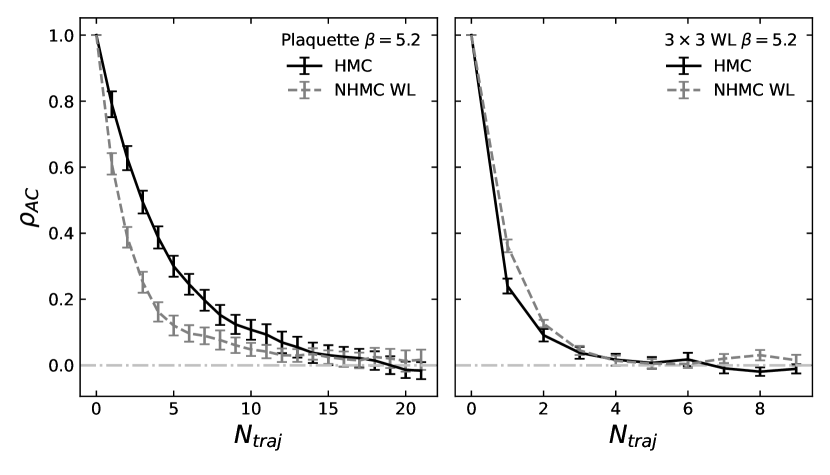
Figure 1: Comparison of the observable autocorrelation $\rho_{\text{AC}}$ plotted as a function of the number of trajectories for the HMC and Nambu HMC with $3\times 3$ Wilson loops (NHMC WL). The left and right plots are the autocorrelation of the plaquette and $3\times 3$ Wilson loop, respectively. This test is performed at $\beta=5.2$ for 315 gauge link updates per trajectory for 5000 trajectories. For the HMC, this corresponds to a total trajectory length of $t=9.9$ with acceptance rate $0.779$ and for the NHMC WL, a total trajectory of length $t=6.75$ with acceptance rate $0.728$.

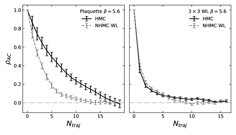
Figure 2: Comparison of the observable autocorrelation $\rho_{\text{AC}}$ plotted as a function of the number of trajectories for the HMC and Nambu HMC with $3\times 3$ Wilson loops (NHMC WL). The left and right plots are the autocorrelation of the plaquette and $3\times 3$ Wilson loop, respectively. This test is performed at $\beta=5.6$ for 315 gauge link updates per trajectory for 5000 trajectories. For the HMC, this corresponds to a total trajectory length of $t=9.0$ with acceptance rate $0.785$ and for the NHMC WL, a trajectory length of $t=5.85$ with acceptance rate $0.787$.

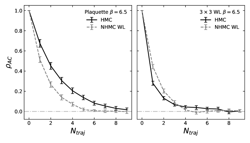
Figure 3: Comparison of the observable autocorrelation $\rho_{\text{AC}}$ plotted as a function of the number of trajectories for the HMC and Nambu HMC with $3\times 3$ Wilson loops (NHMC WL). The left and right plots are the autocorrelation of the plaquette and $3\times 3$ Wilson loop, respectively. This test is performed at $\beta=6.5$ for 360 gauge link updates per trajectory for 5000 trajectories. For the HMC, this corresponds to a total trajectory length of $t=7.2$ with acceptance rate $0.868$ and for the NHMC WL, a trajectory of length $t=5.4$ with acceptance rate $0.818$.

In this test I choose the second auxiliary Hamiltonian to contain the function of $3\times 3$ Wilson loops in Eq. (44) with parameters $\gamma=1.0$ and $\kappa=3.0$. Here, I have not made a careful tuning to optimize the algorithm and the parameters entering the tests have been chosen to obtain a high acceptance rate for long trajectories. To compare the algorithms the discrete time step $\tau$ is adjusted until the algorithms have similar acceptance rates; trajectories are completed using an equivalent number of gauge link updates. The lattices are all initialized from a cold start in which all links are set to identity. Tests measuring the autocorrelations of the plaquette and $3\times 3$ Wilson loops are performed at $\beta=5.2$ , $5.6$ and $6.5$ for a variety of trajectory lengths. For this lattice size $\beta=5.2$ is just below the confining phase transition occurring around $\beta=5.6$, while $\beta=6.5$ is in the deconfined phase. The results for these tests can be found in Figs 1-3. For all tests the results for the plaquette and $3\times 3$ Wilson loop values agree between the algorithms within statistical error. In all tests I find that the Nambu HMC with Wilson loops produces more rapid plaquette decorrelation than the HMC. Futhermore, the algorithm does exert a noticeable effect on the autocorrelation of the long-distance observable while giving the correct plaquette and observable value, as desired.

VI Conclusion

I have presented a novel generalization of the HMC algorithm which uses Nambu mechanics for its MD trajectories, along with a suitable discretization for lattice gauge theory. This formalism allows me to introduce an arbitrary amount of non-locality into the MD while still recovering a target probability distribution, a feature which may be useful for reducing CSD in lattice QCD simulations. In comparison with the standard HMC algorithm in pure $SU(3)$ gauge theory I find that the Nambu HMC produces results consistent with an exact algorithm, while more rapidly decorrelating plaquette values and exerting an influence on the long-distance behavior of the gauge field.

This algorithm can accommodate dynamical fermions in the same manner as the usual HMC and since it requires no additional fermion force evaluations its cost will likely not greatly exceed the usual HMC. This makes the Nambu HMC a particularly economical way to include communication across large lattice distances. Along with adding fermions, the logical next step is to identify a set of non-local observables whose forces may be helpful in reducing critical slowing down in lattice QCD simulations, a direction that is currently under investigation.

Appendix A Proof of detailed balance

This section proves that an extended HMC algorithm using Nambu mechanics for MD steps satisfies the detailed balance condition

$$P(U)P_{T}(U\rightarrow U^{\prime})=P(U^{\prime})P_{T}(U^{\prime}\rightarrow U).$$ (52)

For the purposes of this proof the Hamiltonian $H(U,p,r)$ to be used in the Metropolis accept/reject step is as in Eq. (28)

$$H(U,p,r)=\frac{p^{2}}{2}+\frac{r^{2}}{2}+S(U).$$ (53)

The form of the second auxiliary Hamiltonian $G$ is the same as in the main text. That is, $G(U,p,r)$ is the separable sum of an arbitrary function of the gauge links $f(U)$ and polynomials in $p$ and $r$, subject to the condition that $G(U,p,r)=G(U,-p,r)$. The proof proceeds nearly identically to the one used for the usual HMC [1]. Recall that in accordance with the form of $H(U,p,r)$, at the beginning of each trajectory the fictitious variables $p(x,\mu,i)$ and $r(x,\mu,i)$ are generated at random from a Gaussian distribution $P_{G}(p)$ and $P_{G}(r)$ where

$$P_{G}(z)\propto\exp(-\frac{1}{2}z^{2}).$$ (54)

With $z^{2}$ given by Eq. (29). The MD trajectories are simulated for a total computer time $t$ and at the end of a trajectory one performs a Metropolis accept/reject test with acceptance probability min$(1,e^{-\Delta H})$.

Evolution via Nambu’s evolution equations for time $t$ is a map in phase space $(U(0),p(0),r(0))\rightarrow(U(t),p(t),r(t))$. The probability for choosing a particular point in phase space $(U^{\prime},p^{\prime},r^{\prime})$ is

$$P_{H}\left[(U,p,r)\rightarrow(U^{\prime},p^{\prime},r^{\prime})\right]=\delta\left[(U^{\prime},p^{\prime},r^{\prime})-(U(t),p(t),r(t))\right].$$ (55)

The probability of accepting this change is given by

$$P_{A}\left[(U,p,r)\rightarrow(U^{\prime},p^{\prime},r^{\prime})\right]=\text{min}(1,e^{-\Delta H}),$$ (56)

where $\Delta H=H(U^{\prime},p^{\prime},r^{\prime})-H(U,p,r)$. Together, Eqs. (54-56) yield a probability of transition for the gauge field of

$$P_{T}(U\rightarrow U^{\prime})=\int[dp][dp^{\prime}][dr][dr^{\prime}]P_{G}(p)P_{G}(r)P_{H}\left[(U,p,r)\rightarrow(U^{\prime},p^{\prime},r^{\prime})\right]P_{A}\left[(U,p,r)\rightarrow(U^{\prime},p^{\prime},r^{\prime})\right].$$ (57)

A necessary condition for detailed balance is that the evolution be reversible. As explained in Section III, with the choice of Nambu’s evolution equations with $H(U,p,r)$ given in Eq. (53) and $G(U,p,r)$ of the form stated above, the reverse trajectory is obtained by taking $p(x,\mu,i)\rightarrow-p(x,\mu,i)$ so that

$$P_{H}\left[(U,p,r)\rightarrow(U^{\prime},p^{\prime},r^{\prime})\right]=P_{H}\left[(U^{\prime},-p^{\prime},r^{\prime})\rightarrow(U,-p,r)\right].$$ (58)

Given the properties

$$\exp(-H(U,p,r))\text{min}(1,e^{-\Delta H})=\exp(-H(U^{\prime},p^{\prime},r^{\prime}))\text{min}(e^{\Delta H},1),$$ (59)

and

$$P_{G}(p)P_{G}(r)P(U)\propto\exp(-H(U,p,r)),$$ (60)

the following is true

$$P_{G}(p)P_{G}(r)P(U)P_{A}\left[(U,p,r)\rightarrow(U^{\prime},p^{\prime},r^{\prime})\right] =P_{G}(p^{\prime})P_{G}(r^{\prime})P(U^{\prime})P_{A}\left[(U^{\prime},p^{\prime},r^{\prime})\rightarrow(U,p,r)\right]$$ (61)

$$=P_{G}(-p^{\prime})P_{G}(r^{\prime})P(U^{\prime})P_{A}\left[(U^{\prime},-p^{\prime},r^{\prime})\rightarrow(U,-p,r)\right].$$

Multiplying by $P_{H}$ and integrating over the fictitious momenta one finds

$$\int[dp][dp^{\prime}][dr][dr^{\prime}] P(U)P_{G}(p)P_{G}(r)P_{H}\left[(U,p,r)\rightarrow(U^{\prime},p^{\prime},r^{\prime}))\right]P_{A}\left[(U,p,r)\rightarrow(U^{\prime},p^{\prime},r^{\prime})\right]$$ (62)

$$=\int[d(-p)][d(-p^{\prime})][dr][dr^{\prime}]P(U^{\prime})P_{G}(-p^{\prime})P_{G}(r^{\prime})P_{H}\left[(U^{\prime},-p^{\prime},r^{\prime})\rightarrow(U,-p,r)\right]P_{A}\left[(U^{\prime},-p^{\prime},r^{\prime})\rightarrow(U,-p,r)\right].$$

Considering the invariance of the measure $[dp][dp^{\prime}]=[d(-p)][d(-p^{\prime})]$, this is the detailed balance condition in Eq. (52).

References

- Duane et al. [1987] S. Duane, A. Kennedy, B. J. Pendleton, and D. Roweth, Hybrid monte carlo, Physics Letters B 195, 216 (1987).
- Davies et al. [1990] C. T. H. Davies, G. G. Batrouni, G. R. Katz, A. S. Kronfeld, G. P. Lepage, P. Rossi, B. Svetitsky, and K. G. Wilson, Fourier acceleration in lattice gauge theories. iii. updating field configurations, Phys. Rev. D 41, 1953 (1990).
- Schaefer et al. [2011] S. Schaefer, R. Sommer, and F. Virotta, Critical slowing down and error analysis in lattice qcd simulations, Nuclear Physics B 845, 93–119 (2011).
- Nambu [1973] Y. Nambu, Generalized hamiltonian dynamics, Phys. Rev. D 7, 2405 (1973).
- Kennedy et al. [2013] A. D. Kennedy, P. J. Silva, and M. A. Clark, Shadow hamiltonians, poisson brackets, and gauge theories, Physical Review D 87, 10.1103/physrevd.87.034511 (2013).
- Takhtajan [1994] L. Takhtajan, On foundation of the generalized nambu mechanics, Communications in Mathematical Physics 160, 295 (1994).
- Leimkuhler and Reich [2005] B. Leimkuhler and S. Reich, Simulating Hamiltonian Dynamics, Cambridge Monographs on Applied and Computational Mathematics (Cambridge University Press, 2005).
- Duane et al. [1986] S. Duane, R. Kenway, B. J. Pendleton, and D. Roweth, Acceleration of gauge field dynamics, Physics Letters B 176, 143 (1986).
- Lüscher [2010] M. Lüscher, Computational strategies in lattice qcd (2010), arXiv:1002.4232 [hep-lat] .