Fluctuation-Dissipation Theorem and Information Geometry in Open Quantum Systems

Abstract

We propose a fluctuation-dissipation theorem in open quantum systems from an information-theoretic perspective. We define the fidelity susceptibility that measures the sensitivity of the systems under perturbation and relate it to the fidelity correlator that characterizes the correlation behaviors for mixed quantum states. In particular, we determine the scaling behavior of the fidelity susceptibility in the strong-to-weak spontaneous symmetry breaking (SW-SSB) phase, strongly symmetric short-range correlated phase, and the quantum critical point between them. We then provide a geometric perspective of our construction using distance measures of density matrices. We find that the metric of the quantum information geometry generated by perturbative distance between density matrices before and after perturbation is generally non-analytic. Finally, we design a polynomial proxy that can in principle be used as an experimental probe for detecting the SW-SSB and phase transition through quantum metrology. In particular, we show that each term of the polynomial proxy is related to the Rényi versions of the fidelity correlators.

Introduction – The concept of spontaneous symmetry breaking (SSB) is one of the organizing principles in modern condensed matter physics [1, 2]. SSB in pure state and thermal states are well-understood. Meanwhile, a mixed quantum state $\rho$ admits two classes of global symmetries [3, 4, 5, 6, 7, 8, 9, 10, 11, 12, 13, 14, 15, 16, 17, 18, 19, 20, 21, 22, 23, 24, 25]: one is the strong symmetry defined as $U\rho=e^{i\theta}\rho$ where $U$ is the global symmetry transformation, i.e. every eigenstate of the density matrix carries the same charge under the symmetry; the other is the weak symmetry, defined as $U\rho U^{\dagger}=\rho$, which means that different eigenstates of the density matrix are still the eigenstates of the global symmetry charge, but they may carry different eigenvalues of the symmetry charge. Recently, a new type of SSB pattern, dubbed strong-to-weak SSB (SW-SSB), has been found in mixed states [9, 26, 27, 28, 20, 29, 30, 31, 32, 33, 34, 35], where a strong global symmetry is spontaneously broken down to a weak one. It was proposed that the most proper definition of the SW-SSB state [27] is through the fidelity correlator, namely

$$F\left(\rho,O_{i}O_{j}^{\dagger}\rho O_{j}O_{i}^{\dagger}\right)\sim O(1),$$ (1)

where $F(\rho,\sigma)=(\operatorname{tr}\sqrt{\sqrt{\rho}\sigma\sqrt{\rho}})^{2}$ is the fidelity of two mixed-state density matrices $\rho$ and $\sigma$ and $O_{i}$ is a local operator carrying charges of the strong symmetry. This definition through fidelity correlator ensures that the SW-SSB state is a robust mixed state phase, in the sense that it cannot be “two-way” connected to a symmetric state through symmetric finite or log-depth local quantum channels [27]. Meanwhile, the linear correlator $\operatorname{tr}\left(\rho O_{i}^{\dagger}O_{j}\right)$, broadly used as the diagnosis for SSB in pure and mixed states, is short-ranged for the SW-SSB states.

In quantum many-body physics, symmetry-breaking orders are rigorously studied via the linear response theory [36, 37], where the sensitivity of the order parameter to external perturbation, i.e. the susceptibility, is proportional to the linear correlator of local charged operators. This is colloquially known as the fluctuation-dissipation theorem [38, 39, 40]. However, as the linear correlator for the SW-SSB phase is short-ranged, such an ordered state will not be detected through the conventional linear response theory. This calls for a new formalism to probe mixed quantum states with strong symmetries.

We begin by defining a fidelity-based “magnetization”, whose susceptibility under external perturbation via a quantum channel, is then shown to be related to the fidelity correlator (1). This generalizes the fluctuation-dissipation theorem on the level of fidelity. The fidelity susceptibility diverges linearly with increasing system size in the SW-SSB phase and remains finite in the symmetric short-range correlated phase. At the quantum critical point or intermediate phase between the two phases, the fidelity susceptibility either remains finite or scales sub-linearly with system size.

We then consider the response of the mixed state to external perturbation from the viewpoint of quantum information geometry, where the effect of the perturbation is quantified by the Bures distance between perturbed and unperturbed density matrices. We find that the metric of the information geometry is generally non-analytic, and encodes the correlation behavior of the state. Finally, we provide proxies of the fidelity susceptibility that involve only polynomials of the density matrix $\rho$, which facilitates experimental measurement of the fidelity susceptibility.

Fidelity magnetization and susceptibility – Motivated by the form of the fidelity correlator (1), we define the fidelity magnetization of a mixed-state $\rho$ as

$$M_{F}(\rho):=\frac{1}{N}\sum_{i}F\left(\rho,O_{i}^{\dagger}\rho O_{i}\right),$$ (2)

where $N$ is the total number of sites in the system, and $O^{\dagger}_{i}$ is the charge creation operator. In this work, we will take the U(1) or $\mathbb{Z}_{n}$ symmetry as examples, as the charge creation operator $O^{\dagger}$ of the U(1) and $\mathbb{Z}_{n}$ symmetry can also serve as the order parameter of the symmetry, and they can be made unitary, which ensures that $O^{\dagger}_{i}\rho O_{i}$ is a valid density matrix. If $\rho=\ket{\psi}\bra{\psi}$ is a pure state, the fidelity magnetization reduces to the square of traditional magnetization: $\frac{1}{N}\sum_{i}|\bra{\psi}O_{i}^{\dagger}\ket{\psi}|^{2}$. We subsequently define the fidelity susceptibility as the change of the fidelity magnetization when $\rho$ is perturbed by the following local charge-dephasing quantum channel:

$$\mathcal{E}=\circ_{j}\mathcal{E}_{j},~{}\mathcal{E}_{j}[\rho]=(1-p)\rho+pO_{j}\rho O_{j}^{\dagger},$$ (3)

which reads

$$\chi_{F} =\lim_{p\rightarrow 0}\frac{M_{F}(\mathcal{E}(\rho))-M_{F}(\rho)}{p}$$

$$=\frac{1}{N}\sum_{i}\lim_{p\rightarrow 0}\frac{F\left(\mathcal{E}[\rho],O_{i}^{\dagger}\mathcal{E}[\rho]O_{i}\right)-F\left(\rho,O_{i}^{\dagger}\rho O_{i}\right)}{p}.$$ (4)

The unitarity of $O_{i}$ ensures that $O^{\dagger}_{i}\rho O_{i}$ is a valid density matrix, and Eq. (3) is a valid quantum channel.

For a density matrix with strong global symmetry, the fidelity magnetization $M_{F}(\rho)$ vanishes, and the fidelity susceptibility can be computed as

$$\chi_{F} =\lim_{p\to 0}\frac{1}{Np}\sum_{i}\left[F\left((1-p)^{N}\rho+p(1-p)^{N-1}\sum\limits_{j}O_{j}\rho O_{j}^{\dagger},\ \ (1-p)^{N}O_{i}^{\dagger}\rho O_{i}+p(1-p)^{N-1}\sum_{j}O_{i}^{\dagger}O_{j}\rho O_{j}^{\dagger}O_{i}\right)+O(p^{2})\right]$$ (5)

$$=\lim_{p\to 0}(1-p)^{2N-1}\sum_{i}\left[\sqrt{F}\left(\rho,\frac{1}{N}\sum_{j}O_{i}^{\dagger}O_{j}\rho O_{j}^{\dagger}O_{i}\right)+\sqrt{F}\left(\frac{1}{N}\sum_{j}O_{j}\rho O_{j}^{\dagger},O_{i}^{\dagger}\rho O_{i}\right)\right]^{2}=\eta\sum_{i}F\left(\rho,\frac{1}{N}\sum_{j}O_{i}^{\dagger}O_{j}\rho O_{j}^{\dagger}O_{i}\right),$$

where we use the additivity of fidelity between density matrices with strong symmetries, and take square of Eq.S1 in the supplementary material (SM) [51]. We note here that we have assumed $p\ll 1/N$ in the derivation. The factor $\eta=4$ when $O$ is a $\mathbb{Z}_{2}$ order parameter (i.e., $O^{\dagger}=O$), for instance when $O$ is the charge-$n$ creation operator of a $Z_{2n}$ symmetry, otherwise $\eta=1$; for more details please refer to the SM [51].

Eq. (5) draws a clear analogy with the fluctuation-dissipation theorem that holds in a variety of physical scenarios: the susceptibility of the fidelity magnetization is related to the fidelity correlator of the operator $O$ across different positions, which quantifies the fluctuation of the mixed state $\rho$ with respect to external channel perturbation. We also note that another definition of susceptibility was given based on the classical Fisher information of a density matrix $\rho$ with respect to an infinitesimal decoherence channel analogous to Eq. (3), and the connection to the Rényi correlator and correlation in the doubled space was made [9].

Fidelity susceptibility of mixed-state phases – We now examine the behavior of the fidelity susceptibility in various mixed-state quantum phases. To proceed, we point out that the fidelity susceptibility can be both lower and upper bounded by the sum of the (square-root) fidelity correlator over the entire system (from now on, we will always assume that the system is translation invariant, therefore the fidelity in the summation in Eq. (5) is independent of $i$ ):

$$\sum_{j}F\left(\rho,O_{i}^{\dagger}O_{j}\rho O_{j}^{\dagger}O_{i}\right)\leq\chi_{F}\leq\left[\sum_{j}\sqrt{F}\left(\rho,O_{i}^{\dagger}O_{j}\rho O_{j}^{\dagger}O_{i}\right)\right]^{2},$$ (6)

where the lower bound is guaranteed by the concavity of fidelity, and the upper bound is proved in the SM [51].

We first discuss the behavior of the fidelity susceptibility in the SSB phase of a global symmetry, including the SW-SSB phase, an intrinsically mixed-state phase with no pure-state analogue. The SSB order is characterized by the long-ranged fidelity correlator (1). In the SSB phase, the lower bound of $\chi_{F}$ in Eq. (6) scales as $\sim O(N)$ due to the long-range nature of the fidelity correlator (1), and $\chi_{F}$ itself is a sum of fidelity over the whole system, which is upper bounded by $N$. Therefore, the susceptibility diverges in the thermodynamic limit $N\to\infty$ with the scaling behavior $\chi_{F}\sim O(N)$. Physically, the divergent susceptibility implies that a local channel perturbation would induce a global change in fidelity magnetization, a clear indication of the spontaneity of symmetry breaking.

On the other hand, we show that the susceptibility does not scale with the system size $N$ in a symmetric short-range correlated (SRC) phase (i.e. the paramagnetic phase) where the fidelity correlator decays exponentially, namely

$$F\left(\rho,O_{i}^{\dagger}O_{j}\rho O_{j}^{\dagger}O_{i}\right)\sim e^{-|i-j|/\xi},$$ (7)

where $|i-j|$ is the spatial distance between $i$ and $j$ and $\xi$ is defined as the fidelity correlation length. In fact, the lower and upper bounds in Eq. (6) are both finite:

$$\chi_{F}\geq\sum_{j}F\left(\rho,O_{i}^{\dagger}O_{j}\rho O_{j}^{\dagger}O_{i}\right)\sim\int\frac{\mathrm{d}^{d}\bm{x}}{a^{d}}e^{-|\bm{x}|/\xi}\sim\left(\frac{\xi}{a}\right)^{d},$$ (8)

where we take the continuous limit $\sum_{j}\to\int\frac{\mathrm{d}^{d}\bm{x}}{a^{d}}$ and $a$ is a typical lattice constant. Meanwhile,

$$\chi_{F}\leq\left[\sum_{j}\sqrt{F}\left(\rho,O_{i}^{\dagger}O_{j}\rho O_{j}^{\dagger}O_{i}\right)\right]^{2}\sim\left(\int\frac{\mathrm{d}^{d}\bm{x}}{a^{d}}e^{-|\bm{x}|/2\xi}\right)^{2}\sim\left(\frac{2\xi}{a}\right)^{2d}.$$ (9)

Both bounds are finite in the SRC phase, where $\xi/a\sim O(1)$.

In principle, the SW-SSB and SRC phases could be separated by either a critical point or an intermediate phase. Here we assume that, in such situation, the fidelity correlator decays algebraically, namely

$$F\left(\rho,O_{i}^{\dagger}O_{j}\rho O_{j}^{\dagger}O_{i}\right)\sim|i-j|^{-\gamma},$$ (10)

where $\gamma$ is some positive exponent. The lower and upper bounds by Eq. (6) now depend on $\gamma$, namely

$$\chi_{F}\geq\sum_{j}F\left(\rho,O_{i}^{\dagger}O_{j}\rho O_{j}^{\dagger}O_{i}\right)\sim\int\frac{\mathrm{d}^{d}\bm{x}}{a^{d}}|\bm{x}|^{-\gamma}\sim\left\{\begin{array}[]{rrr}O(1),\ \gamma>d,\\ \log N,\ \gamma=d,\\ N^{1-\frac{\gamma}{d}},\ \gamma<d,\end{array}\right.$$ (14)

and

$$\chi_{F} \leq\left[\sum_{j}\sqrt{F}\left(\rho,O_{i}^{\dagger}O_{j}\rho O_{j}^{\dagger}O_{i}\right)\right]^{2}$$

$$\sim\left(\int\frac{\mathrm{d}^{d}\bm{x}}{a^{d}}|\bm{x}|^{-\gamma/2}\right)^{2}\sim\left\{\begin{array}[]{rrr}O(1),\ \gamma>2d,\\ \log^{2}N,\ \gamma=2d,\\ N^{2-\frac{\gamma}{d}},\ \gamma<2d.\end{array}\right.$$ (18)

Hence when $\gamma>2d$, $\chi_{F}\sim O(1)$, and when $\gamma<d$, $\chi_{F}$ scales sub-linearly with the system size $N$ as

$$N^{1-\frac{\gamma}{d}}\leq\chi_{F}\leq N.$$ (19)

When $d\leq\gamma\leq 2d$, the exact scaling behavior of the fidelity susceptibility in the intermediate phase depends on the physical details.

Quantum information geometry and susceptibility – We now discuss an alternative quantification of the mixed state’s response to external channel perturbation from the perspective of quantum information geometry, where the perturbation is quantified by geometric distances between perturbed and unperturbed density matrices. A broadly used distance measure between density matrices is the Bures distance, whose square is defined as [52, 53, 54, 55, 56, 57, 58, 59]

$$D_{b}^{2}(\rho,\sigma)=2-2\sqrt{F}(\rho,\sigma),$$ (20)

where $\rho$ and $\sigma$ are two density matrices and $\sqrt{F}$ is the square root fidelity. The second order expansion of the Bures distance $D_{b}^{2}(\rho,\rho+d\rho)$ between a density matrix $\rho$ and a perturbed density matrix $\rho+d\rho$ is known as the Bures metric, which describes the susceptibility of the Bures distance under perturbation, and is generally linked to the physical susceptibility when $d\rho$ is generated by an external perturbation. Barring a sudden change of the rank of $\rho$ under perturbation, the quantum fisher information metric, the central quantity in quantum metrology, is four times the Bures metric[60, 61, 62].

In our case, we define a general space-varying channel perturbation that generalizes Eq. (3):

$$\mathcal{E}_{\bm{\theta}}\equiv\circ_{j}\mathcal{E}_{j},\ \mathcal{E}_{j}[\rho]=\cos^{2}\theta_{j}\rho+\sin^{2}\theta_{j}O_{j}\rho O_{j}^{\dagger},$$ (21)

where $\bm{\theta}=(\theta_{1},\theta_{2},\dots,\theta_{N})$ is an $N$-dimensional vector that parameterizes the channel perturbation as infinitesimal rotations. For convenience, we always assume $\theta_{i}>0$. To characterize the geometry of the mixed states generated by such a parameterized channel, we first consider the following distance $D_{b}^{2}\left(\mathcal{E}_{\bm{\theta}}[\rho],\rho\right)$. However, a straightforward calculation shows that, upon expanding to the second order of $\theta$, we always have

$$D_{b}^{2}\left(\mathcal{E}_{\bm{\theta}}[\rho],\rho\right)=\sum_{i}\theta_{i}^{2}=|\bm{\theta}|^{2},$$ (22)

regardless of physical details of $\rho$. This is simply because $\rho$ has strong symmetry, hence every charged state at the $\theta^{2}$ order generated by the channel perturbation is always orthogonal to the original one, reminiscent of the “orthogonality catastrophe” [63]. Instead, we consider the following quantity between two perturbed density matrices

$$g_{B}\left(\bm{\theta},\bm{\phi}\right)\equiv\frac{D_{b}^{2}\left(\mathcal{E}_{\bm{\theta}}[\rho],\rho\right)+D_{b}^{2}\left(\rho,\mathcal{E}_{\bm{\phi}}[\rho]\right)-D_{b}^{2}\left(\mathcal{E}_{\bm{\theta}}[\rho],\mathcal{E}_{\bm{\phi}}[\rho]\right)}{2}.$$ (23)

If $\bm{\theta}$ and $\bm{\phi}$ were to parameterize a Riemannian manifold, expanding Eq. (23) to the second order of $\theta$ and $\phi$ would yield the metric that defines the inner product of such a manifold: $g_{B}\left(\bm{\theta},\bm{\phi}\right)\sim\sum_{ij}g_{ij}\theta_{i}\phi_{j}$, where $g_{ij}$ is the Riemannian metric. However, we will show that this is only the case when the system is at the SRC fixed point. In fact, away from the SRC fixed point, the metric will generally be a non-analytic function of $\theta_{i}$ and $\phi_{i}$.

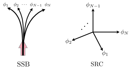
Figure 1: Schematic illustration of quantum information geometry generated by the perturbative channel $\mathcal{E}_{\bm{\phi}}$ in SSB and SRC phases. In the SSB phase, the effective dimension $D_{\text{eff}}$ of the geometry is almost 1-dimensional, since perturbing in any direction $\phi_{i}$ yields the same distance [cf. Eq. (28)], and in the SRC phase different perturbative directions are mostly orthogonal to each other [cf. Eq. (27)].

We investigate the second-order expansion of the Bures metric

$$g_{B}\left(\bm{\theta},\bm{\phi}\right)=\sqrt{F}\left(\sum_{i}\theta_{i}^{2}O_{i}\rho O_{i}^{\dagger},\sum_{j}\phi_{j}^{2}O_{j}\rho O_{j}^{\dagger}\right).$$ (24)

To directly visualize the non-analyticity, we consider the following metric

$$g_{B}\left(\bm{\theta}^{i},\bm{\phi}^{j}+\bm{\phi}^{k}\right)=\sqrt{F}\left(\theta_{i}^{2}O_{i}\rho O_{i}^{\dagger},\phi_{j}^{2}O_{j}\rho O_{j}^{\dagger}+\phi_{k}^{2}O_{k}\rho O_{k}^{\dagger}\right),$$ (25)

where $(\bm{\theta}^{i})_{k}=\theta_{i}\delta_{ik}$ and $(\bm{\phi}^{j})_{k}=\phi_{j}\delta_{jk}$ represent perturbations on one single site. The physical picture of $g_{B}\left(\bm{\theta}^{i},\bm{\phi}^{j}+\bm{\phi}^{k}\right)$ is to turn on two independent perturbations at $j$ and $k$ and measure the system’s response to them at $i$. Using the convexity of Bures distance, we have

$$g_{B}\left(\bm{\theta}^{i},\bm{\phi}^{j}+\bm{\phi}^{k}\right)\leq g_{B}\left(\bm{\theta}^{i},\bm{\phi}^{j}\right)+g_{B}\left(\bm{\theta}^{i},\bm{\phi}^{k}\right).$$ (26)

If $g_{B}$ in Eq. 25 is an analytic function of $\bm{\theta}$ and $\bm{\phi}$, then by definition it can be expanded as a polynomial of $\theta_{i}$ and $\phi_{i}$. However, $g_{B}$ in Eq. 25 is always linear with the amplitude of $\bm{\theta}$ and $\bm{\phi}$, hence this polynomial can only be a linear function of $\phi_{i}$, which would make Eq. 26 an equality rather than inequality. If Eq. 26 is an inequality, it generally implies that $g_{B}$ in Eq. 25 cannot be an analytic function of $\bm{\theta}$ and $\bm{\phi}$. The equality of Eq. 26 holds only when $O_{j}\rho O_{j}^{\dagger}$ is orthogonal to $O_{k}\rho O_{k}^{\dagger}$, i.e. the limit of fixed-point SRC phase. In this case, the Bure metric is

$$g_{B}\left(\bm{\theta},\bm{\phi}\right)\stackrel{{\scriptstyle\text{SRC}}}{{=}}\sum_{i}\theta_{i}\phi_{i}=\bm{\theta}\cdot\bm{\phi},$$ (27)

which is the inner product between two vectors in the $N$-dimensional Euclidean space. Physically, Eq. (26) shows that the response caused by two independent perturbations is not a simple sum of two individual responses, which would be the case in linear response theory.

The non-analyticity of the Bures metric is most drastic in the fixed-point SSB phase, where $O_{i}\rho O_{i}^{\dagger}=O_{j}\rho O_{j}^{\dagger}$ for every $i$ and $j$. The Bures metric becomes

$$g_{B}\left(\bm{\theta},\bm{\phi}\right)\stackrel{{\scriptstyle\text{SSB}}}{{=}}|\bm{\theta}||\bm{\phi}|,$$ (28)

i.e. the entire parameter space collapses into a 1-dimensional flat space. This is because there is only one meaningful perturbation that will be responded by the SSB state: the perturbation that changes the global symmetry charge. We sketch the quantum information geometry of the mixed states generated by the perturbative channel $\mathcal{E}_{\bm{\phi}}$ in Fig. 1.

In general, we can define the effective dimension of the parameter space as

$$D_{\text{eff}}=\frac{N}{\chi_{F}}.$$ (29)

Physically, $D_{\text{eff}}$ counts the number of independent degrees of freedom that are sensitive to the channel perturbation, which can also be roughly estimated as $D_{\text{eff}}\sim V/\xi^{d}$, where $V$ is the system volume and $\xi$ is the fidelity correlation length defined in Eq. (7).

Experimental probe of the fidelity susceptibility – The susceptibility defined in Eq. (5) involves the fidelity between two density matrices, experimental measurement of the fidelity susceptibility calls for the full quantum state tomography (QST) of the density matrix $\rho$. To practically access the fidelity susceptibility, it is more convenient to measure proxies of the fidelity that are polynomials of the density matrix $\rho$. As shown in Ref. [64], the fidelity $F(\rho,\sigma)$ can be lower-bounded by the following inequality:

$$F(\rho,\sigma)\geq\operatorname{tr}(\rho\sigma)+\sqrt{2}\sqrt{\left[\operatorname{tr}(\rho\sigma)\right]^{2}-\operatorname{tr}\left[(\rho\sigma)^{2}\right]}.$$ (30)

Therefore, assuming translation invariance, the fidelity susceptibility can be lower-bounded by

$$\frac{\chi_{F}}{N} =F\left(\rho,\frac{1}{N}\sum_{j}O_{i}^{\dagger}O_{j}\rho O_{j}^{\dagger}O_{i}\right)\geq\frac{1}{N}\sum_{j}\operatorname{tr}\left(\rho O_{i}^{\dagger}O_{j}\rho O_{j}^{\dagger}O_{i}\right)+\sqrt{2}\sqrt{\left[\frac{1}{N}\sum_{j}\operatorname{tr}\left(\rho O_{i}^{\dagger}O_{j}\rho O_{j}^{\dagger}O_{i}\right)\right]^{2}-\operatorname{tr}\left[\left(\frac{1}{N}\sum_{j}\rho O_{i}^{\dagger}O_{j}\rho O_{j}^{\dagger}O_{i}\right)^{2}\right]}.$$ (31)

Such inequality is useful for experimentally tracking a phase transition from an SRC phase to an SSB phase, as the lower bound only contains quantities that are polynomials of $\rho$, which admit more efficient measurement techniques such as classical shadow tomography [65, 66, 67, 68].

Another important consequence of the lower bound in Eq. (30) is that, the Rényi-2 correlator, which is widely used as a theoretical proxy in diagnosing the SRC to SW-SSB phase transition [9, 26, 27, 29], tends to overestimate the SRC phase, and underestimate the SW-SSB phase. This is because a long-ranged Rényi-2 correlator $\operatorname{tr}\left(\rho O_{i}^{\dagger}O_{j}\rho O_{j}^{\dagger}O_{i}\right)$ is a sufficient condition of having a long-ranged fidelity correlator $F\left(\rho,O_{i}^{\dagger}O_{j}\rho O_{j}^{\dagger}O_{i}\right)$ since the latter is always larger. Here we note that in this paper we focus on the 0-form symmetry.

In Supplementary Materials [51], we show that the lower bound in Eq. (30) can be further improved into an increasing sequence that approximates the fidelity, which allows for more accurate experimental estimation of the fidelity susceptibility. Most crucially, we find that the increasing lower bound involves higher Rényi correlators, which are defined as

$$R^{(2n)}\equiv\operatorname{tr}\left[\left(\frac{1}{N}\sum_{j}\rho O_{i}^{\dagger}O_{j}\rho O_{j}^{\dagger}O_{i}\right)^{n}\right].$$ (32)

It is important to point out that the Rényi-$2n$ correlator is also an $(n+1)$-point correlator between the operator $O$, hence it captures a higher moment of fluctuation. In contrast, for pure states, the susceptibility is a simple average of two-point correlators over the entire space.

Conclusion and discussion – In this work, we formulate a fluctuation-dissipation theorem in open quantum system, where fluctuations are quantified by information-theoretic measures. In particular, we find that the susceptibility $\chi_{F}$ of fidelity-based order parameters under external channel perturbation is related to the fidelity correlator, which characterizes the fluctuation in the open quantum system. From the perspective of information geometry, we show that the metric generated by perturbed density matrices encodes correlative behaviors. In particular, it is highly non-analytic when the fidelity susceptibility $\chi_{F}$ diverges. Finally, to facilitate experimental detection of SSB and phase transitions in open quantum systems, we propose polynomial proxies of fidelity susceptibility using Rényi version of the susceptibility, which can be experimentally accessed via classical shadow from randomized measurements. This avoids exponentially hard QST.

We end this work with some open questions. It is well-known that the response of a non-equilibrium quantum many-body system can be studied using the Keldysh formalism. Therefore, it would be meaningful to compare our approach to the response of the quantum sector in the Keldysh formalism to external sources. Another interesting direction is to consider the relation between fidelty susceptibility and our ability to recover the channel perturbation $\mathcal{E}$, which is potentially linked to the spontaneity of SSB states [27]. We leave these studies to future works.

Supplemental Materials for “Fluctuation-Dissipation Theorem and Information Geometry in

Open Quantum Systems”

Appendix S-1 i@. Properties of fidelity and distances

We summarize some useful properties of fidelity, Bures distance and trace distance that are used in the main text and the supplementary material.

1. Additivity: for density matrices $\rho_{i}$, $\sigma_{i}$ and parameters $\lambda_{i},\mu_{i}\in[0,1]$ ($i=1,\cdots,N$),

   $$\begin{gathered}\sqrt{F}\left(\bigoplus_{i=1}^{N}\lambda_{i}\rho_{i},\bigoplus_{i=1}^{N}\mu_{i}\sigma_{i}\right)=\sum_{i=1}^{N}\sqrt{\lambda_{i}\mu_{i}}\sqrt{F}(\rho_{i},\sigma_{i}).\end{gathered}$$ (S2)

   In particular, with the presence of strong global symmetry, the Hilbert space can be decomposed into a direct sum of subspaces with different charges for the global symmetry. Therefore, the additivity applies to summations of density matrices over different global symmetry charges, since the algebraic sum is now equivalent to the direct sum.

2. Concavity: for density matrices $\rho$ and $\sigma_{i}$ ($i=1,\cdots,N$),

   $$\begin{gathered}F\left(\rho,\sum_{i}p_{i}\sigma_{i}\right)\geq\sum_{i}p_{i}F(\rho,\sigma_{i})\end{gathered},$$ (S4)

   where $\{p_{i}\}$ is a probability distribution such that $\sum_{i}p_{i}=1$.

3. Joint concavity: for density matrices $\rho_{i}$ and $\sigma_{i}$ ($i=1,\cdots,N$) with the probability distribution $\{p_{i}\}$,

   $$\begin{gathered}\sqrt{F}\left(\sum_{i}p_{i}\rho_{i},\sum_{i}p_{i}\sigma_{i}\right)\geq\sum_{i}p_{i}\sqrt{F}(\rho_{i},\sigma_{i})\end{gathered}.$$ (S6)

4. Multiplicativity: for density matrices $\rho_{i}$ and $\sigma_{i}$ ($i=1,2$),

   $$\begin{gathered}F(\rho_{1}\otimes\rho_{2},\sigma_{1}\otimes\sigma_{2})=F(\rho_{1},\sigma_{1})F(\rho_{2},\sigma_{2})\end{gathered}.$$ (S8)

5. Data processing inequality: for a completely positive trace-preserving map $\mathcal{E}$ (i.e., quantum channel),

   $$\begin{gathered}F\left(\mathcal{E}[\rho],\mathcal{E}[\sigma]\right)\geq F(\rho,\sigma)\end{gathered}.$$ (S10)

Appendix S-2 ii@. Upper bound of the fidelity susceptibility in Eq. (6)

In this section, we prove that the upper bound in Eq. (6). To this end, we first note that, for positive definite matrices $A$ and $B$ of the same dimension, the following inequality holds:

$$\operatorname{tr}\sqrt{A+B}\leq\operatorname{tr}\sqrt{A}+\operatorname{tr}\sqrt{B}.$$ (S11)

This is known as Ando’s inequality in the context of operator monotone functions [69, 70].

Applying Eq. (S11) recursively, we arrive at the following inequality: for positive semi-definite matrices $M_{i}$ of the same dimension, $i=1,2,\dots,N$, we have

$$\operatorname{tr}\left(\sqrt{\sum_{i=1}^{N}M_{i}}\right)\leq\sum_{i=1}^{N}\operatorname{tr}\sqrt{M_{i}}.$$ (S12)

Now consider the fidelity susceptibility. Assuming translation invariance, we have

$$\chi_{F} =N\cdot F\left(\rho,\frac{1}{N}\sum_{j}O_{i}^{\dagger}O_{j}\rho O_{j}^{\dagger}O_{i}\right)=N\left(\operatorname{tr}\sqrt{\frac{1}{N}\sum_{j}\sqrt{\rho}O_{i}^{\dagger}O_{j}\rho O_{j}^{\dagger}O_{i}\sqrt{\rho}}\right)^{2}$$

$$\leq\left(\sum_{j}\operatorname{tr}\sqrt{\sqrt{\rho}O_{i}^{\dagger}O_{j}\rho O_{j}^{\dagger}O_{i}\sqrt{\rho}}\right)^{2}=\left(\sum_{j}\sqrt{F}\left(\rho,O_{i}^{\dagger}O_{j}\rho O_{j}^{\dagger}O_{i}\right)\right)^{2},$$ (S13)

where the inequality holds from Eq. (S12) and the fact that the matrix $\sqrt{\rho}O_{i}^{\dagger}O_{j}\rho O_{j}^{\dagger}O_{i}\sqrt{\rho}$ is positive semi-definite.

Appendix S-3 iii@. Derivation of Eq. (5) for $\mathbb{Z}_{2}$ order parameter

Distinct from other charged local operators, the $\mathbb{Z}_{2}$ order parameter satisfies $O^{\dagger}=O$. So for a $\mathbb{Z}_{2}$ order parameter, the corresponding fidelity susceptibility is slightly different, namely (again, we assume translation invariance)

$$\chi_{F}= \lim_{p\rightarrow 0}\frac{1}{p}F\left((1-p)^{N}\rho+p(1-p)^{N-1}\sum_{j}O_{j}\rho O_{j}+p^{2}(1-p)^{N-2}\sum_{j,k}O_{j}O_{k}\rho O_{k}O_{j},(1-p)^{N}O_{i}\rho O_{i}+p(1-p)^{N-1}\sum_{j}O_{i}O_{j}\rho O_{j}O_{i}\right)+\mathcal{O}(p)$$

$$= \lim_{p\rightarrow 0}\frac{1}{p}F\left((1-p)^{N}\rho+p^{2}(1-p)^{N-2}\sum_{j,k}O_{j}O_{k}\rho O_{k}O_{j},\ \ p(1-p)^{N-1}\sum_{j}O_{i}O_{j}\rho O_{j}O_{i}\right)$$

$$+\lim_{p\rightarrow 0}\frac{1}{p}F\left(p(1-p)^{N-1}\sum_{j}O_{j}\rho O_{j},\ \ (1-p)^{N}O_{i}\rho O_{i}\right)$$

$$+\lim_{p\rightarrow 0}\frac{2}{p}\sqrt{F}\left((1-p)^{N}\rho+p^{2}(1-p)^{N-2}\sum_{j,k}O_{j}O_{k}\rho O_{k}O_{j},p(1-p)^{N-1}\sum_{j}O_{i}O_{j}\rho O_{j}O_{i}\right)\sqrt{F}\left(p(1-p)^{N-1}\sum_{j}O_{j}\rho O_{j},(1-p)^{N}O_{i}\rho O_{i}\right)$$

$$= \lim_{p\rightarrow 0}(1-p)^{2N-1}F\left(\rho+\left(\frac{p}{1-p}\right)^{2}\sum_{j,k}O_{j}O_{k}\rho O_{k}O_{j},\sum_{j}O_{i}O_{j}\rho O_{j}O_{i}\right)+\lim_{p\rightarrow 0}(1-p)^{2N-1}F\left(\sum_{j}O_{j}\rho O_{j},O_{i}\rho O_{i}\right)$$

$$+\lim_{p\rightarrow 0}2(1-p)^{2N-1}\sqrt{F}\left(\rho+\left(\frac{p}{1-p}\right)^{2}\sum_{j,k}O_{j}O_{k}\rho O_{k}O_{j},\sum_{j}O_{i}O_{j}\rho O_{j}O_{i}\right)\sqrt{F}\left(\sum_{j}O_{j}\rho O_{j},O_{i}\rho O_{i}\right).$$ (S14)

In particular, we note that the first term of the above equation can be both upper and lower bounded simultaneously, namely

$$F \left(\rho+\left(\frac{p}{1-p}\right)^{2}\sum_{j,k}O_{j}O_{k}\rho O_{k}O_{j},\sum_{j}O_{i}O_{j}\rho O_{j}O_{i}\right)$$

$$\geq F\left(\rho,\sum_{j}O_{i}O_{j}\rho O_{j}O_{i}\right)+\left(\frac{p}{1-p}\right)^{2}F\left(\sum_{j,k}O_{j}O_{k}\rho O_{k}O_{j},\sum_{j}O_{i}O_{j}\rho O_{j}O_{i}\right),$$ (S15)

and

$$F \left(\rho+\left(\frac{p}{1-p}\right)^{2}\sum_{j,k}O_{j}O_{k}\rho O_{k}O_{j},\sum_{j}O_{i}O_{j}\rho O_{j}O_{i}\right)$$

$$\leq\left[\sqrt{F}\left(\rho,\sum_{j}O_{i}O_{j}\rho O_{j}O_{i}\right)+\frac{p}{1-p}\sqrt{F}\left(\sum_{j,k}O_{j}O_{k}\rho O_{k}O_{j},\sum_{j}O_{i}O_{j}\rho O_{j}O_{i}\right)\right]^{2},$$ (S16)

where we have applied Eq. (S12). We notice that both upper and lower bounds converge to the fidelity $F\left(\rho,\sum_{j}O_{i}O_{j}\rho O_{j}O_{i}\right)$ in the limit $p\to 0$. Therefore, for $\mathbb{Z}_{2}$ order parameter, the fidelity susceptibility will have a prefactor 4, namely

$$\chi_{F}^{\mathbb{Z}_{2}}=4N\cdot F\left(\rho,\frac{1}{N}\sum_{j}O_{i}O_{j}\rho O_{j}O_{i}\right).$$ (S17)

Appendix S-4 iv@. Converging lower bounds for fidelity

In this section, we provide the construction of a converging series of lower bounds, each consisting of polynomials of the density matrices, that approximates the fidelity between two density matrices. This improves the lower bound provided by Ref. [64].

We begin by expanding the fidelity as following:

$$F(\rho,\sigma)=\left[\operatorname{tr}\left(\sqrt{\sqrt{\rho}\sigma\sqrt{\rho}}\right)\right]^{2}=\left(\sum_{i}\sqrt{\lambda_{i}}\right)^{2},$$ (S18)

where $\lambda_{i}$ is the $i$-th eigenvalue of the matrix $\sqrt{\rho}\sigma\sqrt{\rho}$. We note that, since $\sqrt{\rho}\sigma\sqrt{\rho}$ is similar to $\rho\sigma$ [64, 71], $\{\lambda_{i}\}$ is also the set of eigenvalues of $\rho\sigma$. Expanding the square, we have

$$F(\rho,\sigma) =\sum_{i,j}\sqrt{\lambda_{i}}\sqrt{\lambda_{j}}=\sum_{i}\lambda_{i}+\sum_{i\neq j}\sqrt{\lambda_{i}}\sqrt{\lambda_{j}}$$ (S19)

An increasing lower bound can be achieved as follows. Denoting $F\equiv F(\rho,\sigma)$ and $F_{1}\equiv\sum_{i}\lambda_{i}=\operatorname{tr}(\sqrt{\rho}\sigma\sqrt{\rho})=\operatorname{tr}(\rho\sigma)$, the first lower bound is simply

$$F\geq F_{1}.$$ (S20)

To improve the lower bound, we calculate their difference:

$$\delta F_{1}\equiv(F-F_{1})^{2}=\sum_{i\neq j,k\neq l}\sqrt{\lambda_{i}}\sqrt{\lambda_{j}}\sqrt{\lambda_{k}}\sqrt{\lambda_{l}}=2\sum_{i\neq j}\lambda_{i}\lambda_{j}+\sum_{\langle ij,kl\rangle}\sqrt{\lambda_{i}}\sqrt{\lambda_{j}}\sqrt{\lambda_{k}}\sqrt{\lambda_{l}},$$ (S21)

where $\langle ij,kl\rangle$ denotes the range of the indices to be $i\neq j,k\neq l/\{i=k,j=l\text{ or }i=l,j=k\}$. To proceed, we define

$$F_{2}\equiv\sum_{i\neq j}\lambda_{i}\lambda_{j}=\left(\sum_{i}\lambda_{i}\right)^{2}-\sum_{i}\lambda_{i}^{2}=\left[\operatorname{tr}(\rho\sigma)\right]^{2}-\operatorname{tr}\left[(\rho\sigma)^{2}\right].$$ (S22)

Then Eq. (S21) gives a better lower bound of the fidelity, $\delta F_{1}\geq 2F_{2}$, which is obtained in Ref. [64]. Moving further, we have

$$\delta F_{2}\equiv\left(\delta F_{1}-2F_{2}\right)^{2}=\sum_{\langle ij,kl\rangle,\langle mn,pq\rangle}\sqrt{\lambda_{i}}\sqrt{\lambda_{j}}\sqrt{\lambda_{k}}\sqrt{\lambda_{l}}\sqrt{\lambda_{m}}\sqrt{\lambda_{n}}\sqrt{\lambda_{p}}\sqrt{\lambda_{q}}=8\sum_{\langle ij,kl\rangle}\lambda_{i}\lambda_{j}\lambda_{k}\lambda_{l}+\cdots,$$ (S23)

where the ellipsis indicates the remaining terms that involve square roots. We similarly define

$$F_{3} =\sum_{\langle ij,kl\rangle}\lambda_{i}\lambda_{j}\lambda_{k}\lambda_{l}=F_{2}^{2}-2\left[\left(\sum_{i}\lambda_{i}^{2}\right)^{2}-\sum_{i}\lambda_{i}^{4}\right]$$ (S24)

$$=\left[\operatorname{tr}(\rho\sigma)\right]^{4}-2\left[\operatorname{tr}(\rho\sigma)\right]^{2}\operatorname{tr}\left[(\rho\sigma)^{2}\right]-\operatorname{tr}\left[(\rho\sigma)^{2}\right]^{2}+2\operatorname{tr}\left[(\rho\sigma)^{4}\right],$$

so that $\delta F_{2}\geq 8F_{3}.$

It is clear from the above derivations that the inequality can be iterated to provide even closer lower bounds of fidelity. In general, for every $n>1$, we have the following recursion

$$\delta F_{n}\equiv\left[\delta F_{n-1}-2^{\frac{n(n-1)}{2}}F_{n}\right]^{2}\geq 2^{\frac{n(n+1)}{2}}F_{n+1},$$ (S25)

where

$$F_{n+1}=F_{n}^{2}-2^{\frac{n(n-1)}{2}}\left[\left(\sum_{i}\lambda_{i}^{2^{n-1}}\right)^{2}-\sum_{i}\lambda_{i}^{2^{n}}\right].$$ (S26)

Using these relations, the fidelity can be represented by the following exact form:

$$F=F_{1}+\sqrt{2F_{2}+\sqrt{8F_{3}+\sqrt{\cdots\sqrt{2^{\frac{n(n-1)}{2}}F_{n}+\sqrt{\cdots}}}}}.$$ (S27)

In our case, the fidelity is between the system’s density matrix $\rho$ and $\sigma=\frac{1}{N}\sum_{j}O_{i}^{\dagger}O_{j}\rho O_{j}^{\dagger}O_{i}$. Therefore, the fidelity proxy $F_{n}$ involves the Rényi-$2^{n}$ correlator

$$R^{(2n)}(i,j)=\operatorname{tr}\left[\left(\frac{1}{N}\sum_{j}\rho O_{i}^{\dagger}O_{j}\rho O_{j}^{\dagger}O_{i}\right)^{2^{n-1}}\right].$$ (S28)