soft open fences
Two-dimensional Stoner transitions beyond mean-field
Abstract
We have previously shown that the Stoner instability 2D has unconventional behavior: it is strongly first order but features a susceptibility which diverges at the transition point. Here, we analyze the Stoner transition for two-dimensional systems with spin and valley degrees of freedom, beyond mean field. At low density, we show that in one-valley and isotropic two-valley systems the leading effect beyond mean-field theory is suppression of the Stoner instability. In anisotropic two-valley systems, we show that, for larger anisotropy, the transition remains mean-field-like and retains its unconventional properties. We discuss applications to AlAs quantum wells.
I Introduction
For nearly the two decades since the experimental fabrication of graphene, there has been broad experimental interest in quasi- two-dimensional (2D) semiconductors whose low-energy theory hosts spin and valley degrees of freedom. In this time there have been many proposals for how the valley iso-spin allows for new phenomena and applications, a field given the moniker “valleytronics” [1, 2] in analogy with the spintronic applications of older semiconductors [3].
Interest in systems with such valley and spin degrees of freedom only intensified when superconductivity was discovered in twisted bilayer graphene (TBG) [4, 5, 6] in close proximity to correlated phases, which may possess an isospin order [7].
Since then, several experiments have observed the formation of spontaneously iso-spin polarized states in other quasi-two-dimensional systems with spin and valley degrees of freedom, including non-twisted Bernal-stacked bilayer graphene (BBG), rhombohedral tri-layer graphene (RTG) in displacement field [8, 9, 10, 11, 12, 13, 14, 15, 16, *Blinov2023a] and AlAs quantum wells [18, 19, 20, 21]. These experiments triggered an array of theoretical studies of these systems [22, 23, 24, 25, 26, 27, 28, 29, 30, 31, 27, 29, 32, 33].
Measurements near the onset of spin order in BBG, RTG, and AlAs hint at unconventional behavior: approaching the transition from the unpolarized side, soft-bosonic excitations are observed e.g., a growing static iso-spin susceptibility in AlAs [18, 19]; however, the transitions themselves are strongly first order, with some number of iso-spin bands being completely depopulated immediately below the transition [10, 9, 11, 13, 14, 15, 34, 18, 19, 20, 21].
L. Glazman and the two of us (RGC) recently argued [35, 36] that these unconventional features can be qualitatively reproduced by analyzing iso-spin Stoner transitions in 2D within mean-field (Hartree-Fock) theory for a system of fermions with a repulsive interaction and isotropic dispersion. We demonstrated that in a one-valley system with a parabolic dispersion, the Stoner transition at a critical is a first-order transition into a fully polarized ferromagnetic state, yet it is accompanied by the divergence of the magnetic susceptibility at (see Sec. II below). For a two-valley system with SU(4) symmetry and parabolic dispersion, the Stoner instability is a first-order transition into a fully spin and valley polarized quarter-metal state, again accompanied by the divergence of an iso-spin susceptibility. When SU(4) symmetry is broken, there is a cascade of two first-order transitions, the first one into a half-metal and the second one into a quarter-metal. Like in other cases, each transition is accompanied by a divergence of the corresponding iso-spin susceptibility (Sec. III).
In this work, we extend the previous analysis by going beyond mean-field (MF) and also including the anisotropy of the dispersion. It has been argued earlier that at least in a single-valley system the existence of a ferromagnetic transition beyond the MF level is not guaranteed because particle-particle renormalizations suppress and may keep it below the level required for the Stoner instability [37, 38, 39]. On the other hand, E. Lieb has rigorously shown [40] that a ferromagnetic transition does occur at a finite Hubbard for a single-valley fermionic system on the half-filled Lieb lattice[40], and experiments on BBG, RTG, AlAs, and other materials did show a cascade of transitions, identified as instabilities towards an iso-spin order.
From a general point of view, there are three possibilities beyond MF:
-
(I)
A MF-like transition, perhaps at larger ,
-
(II)
A first-order transition to a polarized state, with no divergence of the susceptibility,
-
(III)
No transition.
In this work, we obtain the leading beyond-MF contributions to the 2D Stoner susceptibility and the ground state energy at low electron density and attempt to distinguish between these three possibilities. We show that in both single-valley and isotropic two-valley systems, the dominant effect beyond MF is a downturn renormalization of the interaction that determines the Stoner instability, by logarithmically large contributions from the particle-particle channel. Treating these logarithmic contributions within the ladder approximation, we find that they suppress the iso-spin susceptibilities and make the iso-spin polarized state energetically unfavorable. This clearly indicates that the MF approximation severely overestimates the system’s ability to develop a Stoner instability. Taken at a face value, these results are consistent with the case (III). However, what actually happens at larger remains an open question because the logarithmic approximation neglects subleading, non-logarithmic corrections in the particle-particle channel, which at large enough may invalidate the logarithmic approximation and allow an iso-spin susceptibility to diverge at some critical (this would be case I). 111An example of such behavior is pairing at a quantum-critical point in a metal and in the Yukawa-SYK model, where ladder series of Cooper logarithms in the pairing vertex do not give rise to an instability, but once the coupling exceeds some critical value, subleading terms invalidate ladder summation, and the system becomes unstable towards pairing (see e.g. Refs. [41, 42]). Also, RPA-type particle-hole corrections to the ground state energy may shift the energy balance in favor of an iso-spin polarized state even if a corresponding iso-spin susceptibility remains finite (this would be case II).
For a two-valley system with an anisotropic quadratic dispersion, like the one in AlAs — two bands centered at the and points in the Brillouin zone (centers of the two valleys) with , where and in the two valleys — SU(4) symmetry is broken already in the MF approximation. Yet, within the MF, the degeneracy between valley polarization and intra-valley ferromagnetism remains, and the Stoner transition within MF is again a first-order transition into a fully polarized, spin/valley ordered quarter-metal state, accompanied by the divergence of an iso-spin susceptibility. Beyond MF, we show in Sec. III.2 that the degeneracy between Stoner transitions into a ferromagnetic state and a valley polarized state is broken. For the ferromagnetic interaction logarithmic corrections from the particle-particle channel are the same as in the isotropic case, and as long as logarithmic approximation is valid, there is no Stoner instability. For the interaction that governs the Stoner transition into a valley polarized state, however, the strength of the logarithmic corrections depends on the anisotropy parameter . For large , we find that the critical , at which the valley polarization susceptibility diverges, is comparable to the MF value. In Sec. III.3, we analyze the ground state energy beyond MF and argue that within the same logarithmic approximation, the system undergoes a first-order transition into fully valley-polarized state at exactly the same . This is scenario I: a MF-like Stoner transition.
We emphasize that our result is based on the summation of ladder series of logarithmical renormalizations from the particle-particle channel both for the susceptibility and for the ground state energy. In a somewhat different approach, the authors of [33] summed up the series of RPA-type ring diagrams for the ground state energy. They found first-order valley polarization and ferromagnetic transitions (in this order), not accompanied by the divergence of the corresponding susceptibilities (scenario II). We compare the two calculations in Sec. IV.
In what follows, we will reserve the designation Stoner for instabilities where the iso-spin susceptibility diverges at the transition point. In this language, MF transitions in a single-valley and a two-valley system are Stoner transitions, while beyond MF the three choices are a Stoner transition, a first-order transition not accompanied by the divergence of the corresponding susceptibility, or no transition at all.
In order to highlight the role played by valley physics, we first consider a single-valley system within and beyond MF, and then do the same analysis for a two-valley system.
II A single-valley system
We consider a model of two-dimensional spin-full fermions with repulsive contact interaction
| (1) |
where indexes spin and is the chemical in absence of interactions.
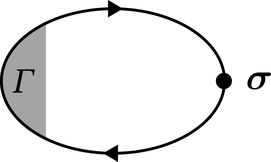
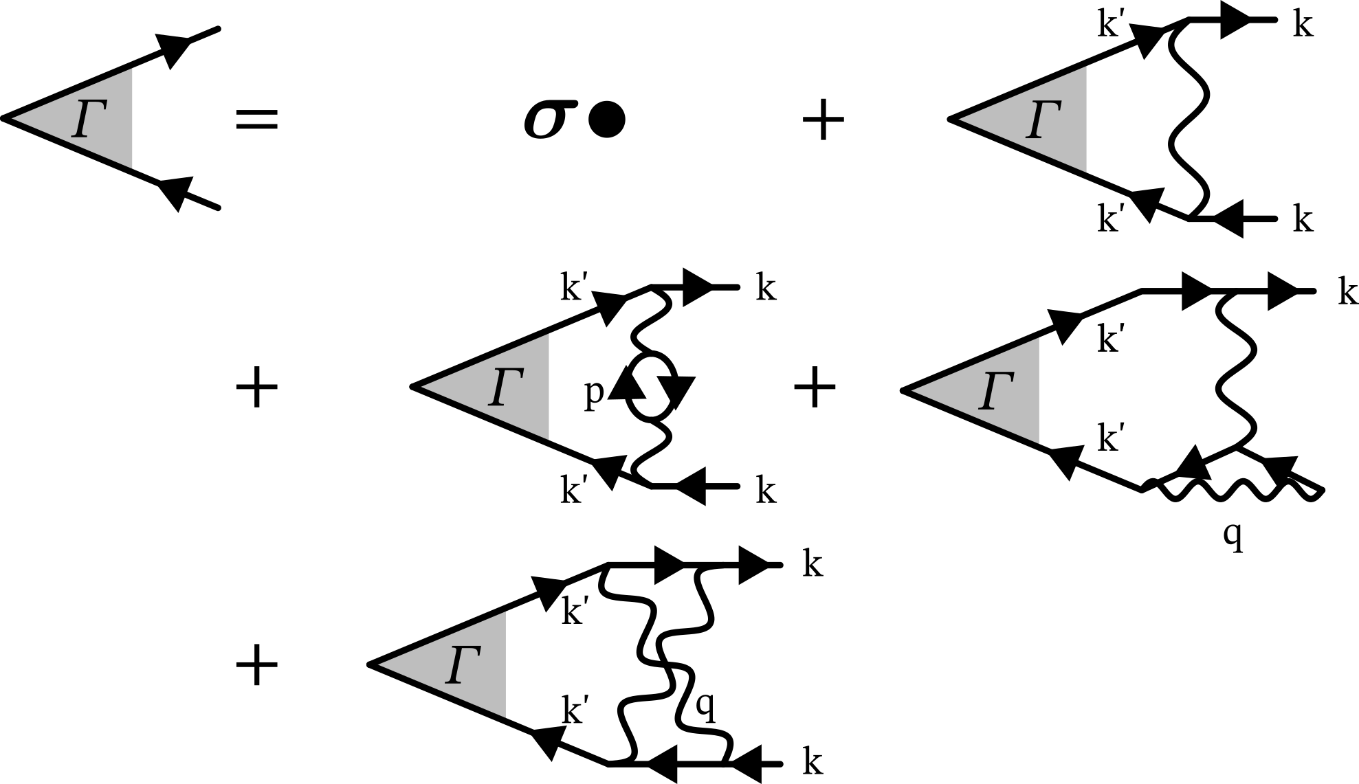
Our goal is to obtain the spin susceptibility in the paramagnetic state and the ground state energy in the presence of a ferromagnetic order. The paramagnetic spin susceptibility is the convolution of wo fermionic propagators and the fully renormalized spin vertex (see Fig. 1)
| (2) |
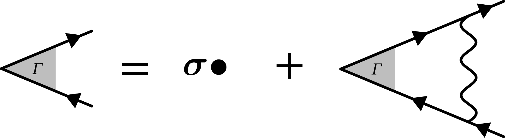
where is the internal momentum and frequency, and is the solution of the Bethe-Salpeter (BS) equation
| (3) |
and where is the fully renormalized irreducible four-point function, which generally has some spin structure.
To calculate the ground state energy one can follow the variational Luttinger-Ward approach [43]. The Luttinger-Ward free energy (ground state energy at )
| (4) |
is a functional of the full Green’s function
and the self-energy is defined by . The Luttinger-Ward functional is obtained by collecting closed-loop diagrams in the loop expansion with the full Green’s functions. Working in terms of the Luttinger-Ward functional has the benefit of automatically producing a self-consistent and conserving approximation [43, 44, 45].
We first review this procedure in the MF approximation and then move beyond MF.
II.1 Spin susceptibility in MF
We start with the normal state susceptibility. The MF approximation uses the bare instead of in (3) and approximates by the bare interaction . This makes independent of . We then have
| (5) |
and
| (6) |
At low temperatures
| (7) |
and the solutions of Eqs. 5 and 6 can then be explicitly written as
| (8) |
The renormalized spin vertex and the spin susceptibility diverge at , signaling the ferromagnetic instability of the normal state.
II.2 Ground state energy in MF
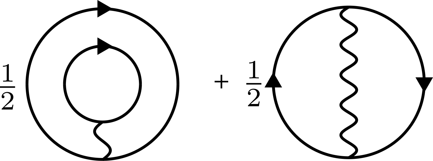
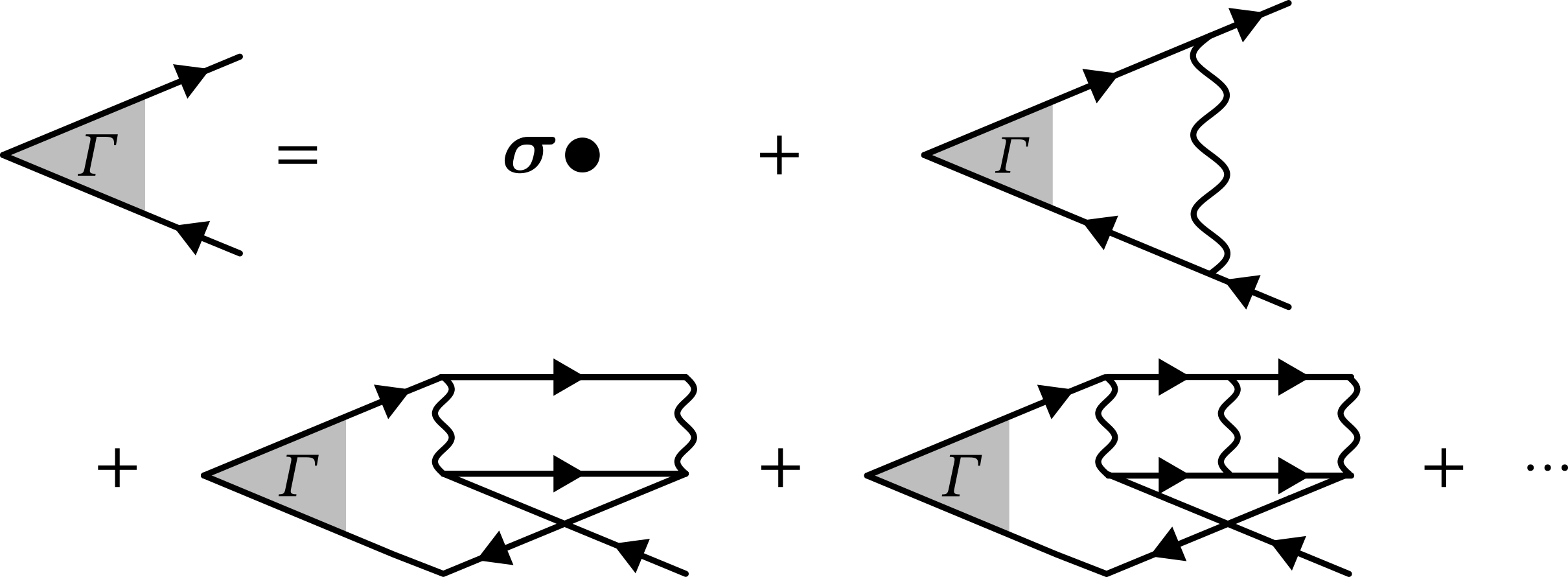
Within the same approximation, one should use only Hartree and Fock diagrams for the Luttinger-Ward functional , see Fig. 3,
| (9) |
Because the corresponding fermionic reduces to a constant, it can be absorbed into the renormalization of the chemical potential from to the actual , related to fermionic density, and a constant shift of the spin-bands relative to each other, related to the spin polarization. One can then easily verify that this approximation is equivalent to evaluating kinetic and potential energies with free-fermion propagators in the presence of spin polarization and keeping only Hartree and Fock diagrams for the potential energy. One can also verify that the MF expression for is obtained by applying a magnetic field and differentiating the ground state energy, obtained this way, twice over the field.
In 2D, the MF ground state energy turns out to be a quadratic function of the dimensionless spin polarization [35, *Raines2024b]
| (10) |
where is the energy of the normal state, is the fixed total density, and . There are no terms of higher order in . This form of indicates that the system undergoes a first order transition to a fully spin-polarized state at , i.e., at exactly the same point where the static spin-susceptibility Eq. 8 diverges. We illustrate this in Fig. 4.
We emphasize that this behavior is a consequence of the fact that the energy is exactly quadratic in the polarization, . 222 For a generic isotropic power-law dispersion , a first order transition of Stoner type develops for both and dispersions ( and ). For intermediate , a first-order transition occurs before the susceptibility diverges, but the difference between the critical where this happens and where the susceptibility would diverge is less than 2% [35, *Raines2024b], i.e., to a truly good approximation, a first-order Stoner transition holds for all power-law dispersions with ..
II.3 Spin susceptibility beyond MF
To go beyond MF, we first ask what the most important contribution is at the next order, i.e., two-loop. In doing so, we will see that for the low-density limit, one of the contributions is universally larger than the other. Concretely, let us look at contributions obtained by keeping irreducible four-point function to two loops. At two-loop order there are three contributions, shown in Fig. 5.
For the Hubbard model, the polarization insertion and vertex correction diagrams (the ones in the second line in Fig. 5) cancel, leaving just the crossed diagram. Even so, let us look at the behavior of each of two-loop diagram. For all diagrams the external fermionic momentum is near the Fermi surface . Additionally, the factor of from the lines adjacent to the vertex means that the dominant contribution comes from . For the polarization insertion and vertex correction diagrams, the restrictions on and are sufficient to restrict other internal fermionic momenta to the vicinity of the Fermi surface. This leads to regular corrections to the vertex, of order , as one can easily verify. The story is qualitatively different for the crossed diagram. Here we have
| (11) |
While the Matsubara sums restrict to be near the Fermi surface, the integration over is unconstrained: because this diagram involves a particle-particle process, all we require is that the intermediate particles both be above or below the Fermi surface. This has strong implications for low-density systems, i.e., those in which can be considered small compared to the upper cutoff of the model, . There is a contribution from leading to a regular term, but there is also a contribution coming from . To evaluate this piece we can, at leading order, neglect the fermionic momenta and the corresponding frequencies compared to and approximate
| (12) |
where we have defined the particle-particle bubble
| (13) |
In the low temperature limit, as noted above, while
| (14) |
This has a familiar form, expected for the particle-particle polarization, but there is a lower cutoff at can no longer be neglected at smaller . The upper cutoff is determined by the UV properties of the model and may take different forms depending on the nature of the underlying lattice model. Since we are considering a Hubbard-like model here, is of order the Brillouin zone size. We now notice that the integral in Eq. 14 is logarithmically singular. This is not a Cooper logarithm as Eq. 14 is only valid at , but rather a 2D-specific logarithm associated with the logarithmic behavior of the scattering amplitude. Evaluating the integral in Eq. 14 to logarithmic accuracy, we find,
| (15) |
For systems with the logarithm is parametrically large.
We can thus approximate the entire two-loop Bethe-Salpeter equation as
| (16) |
where the terms on the right-hand side come from the bare, MF, and crossed contributions respectively. The associated two-loop susceptibility is
| (17) |
We see from Eq. 17 that the leading effect at two-loop order is suppression of the Stoner instability due to particle-particle contributions away from the Fermi surface. Furthermore, from Eq. 17 does not diverge for any value of .
With the insights from two-loop order we can go further. Note that at -loop order, there will be a contribution to the Bethe-Salpeter equation from the maximimally crossed diagram, involving independent particle-particle terms that goes as Any other diagram of the same order in contains at most . Summing only these leading contributions to all orders (see Fig. 6), we find, to logarithmic accuracy,
| (18) |
This is readily solved for
| (19) |
Within the regime , where the logarithmic expansion is controlled we have that and thus the susceptibility does not diverge.
The result may intuitively be understood by noting that in the low density limit each two-particle collision can be considered independent from the other fermions. Thus, the leading effect may be captured by replacing the bare interaction with the two-particle scattering amplitude, which is logarithmically singular in 2D [46, 47, 48].
II.4 Ground state energy beyond MF
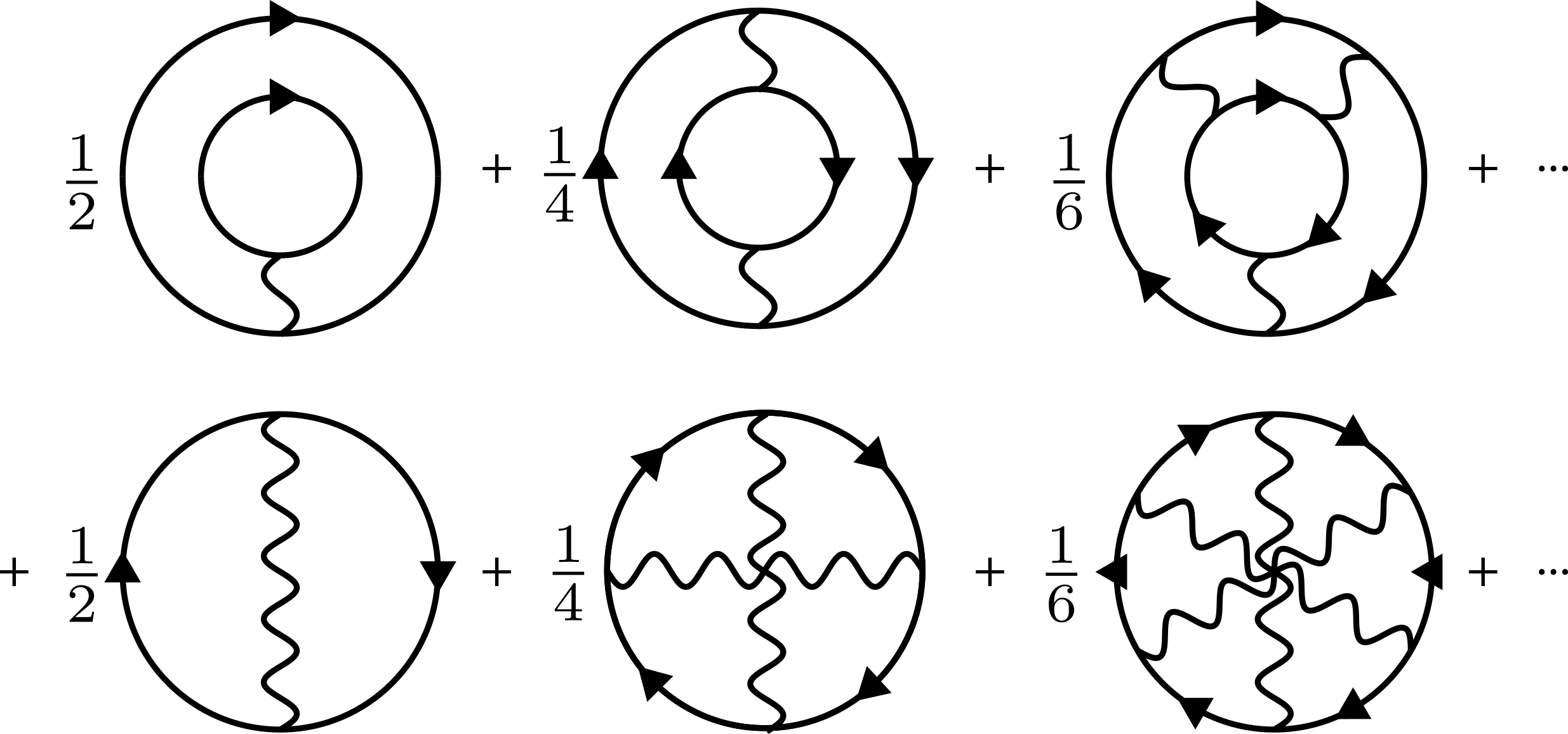
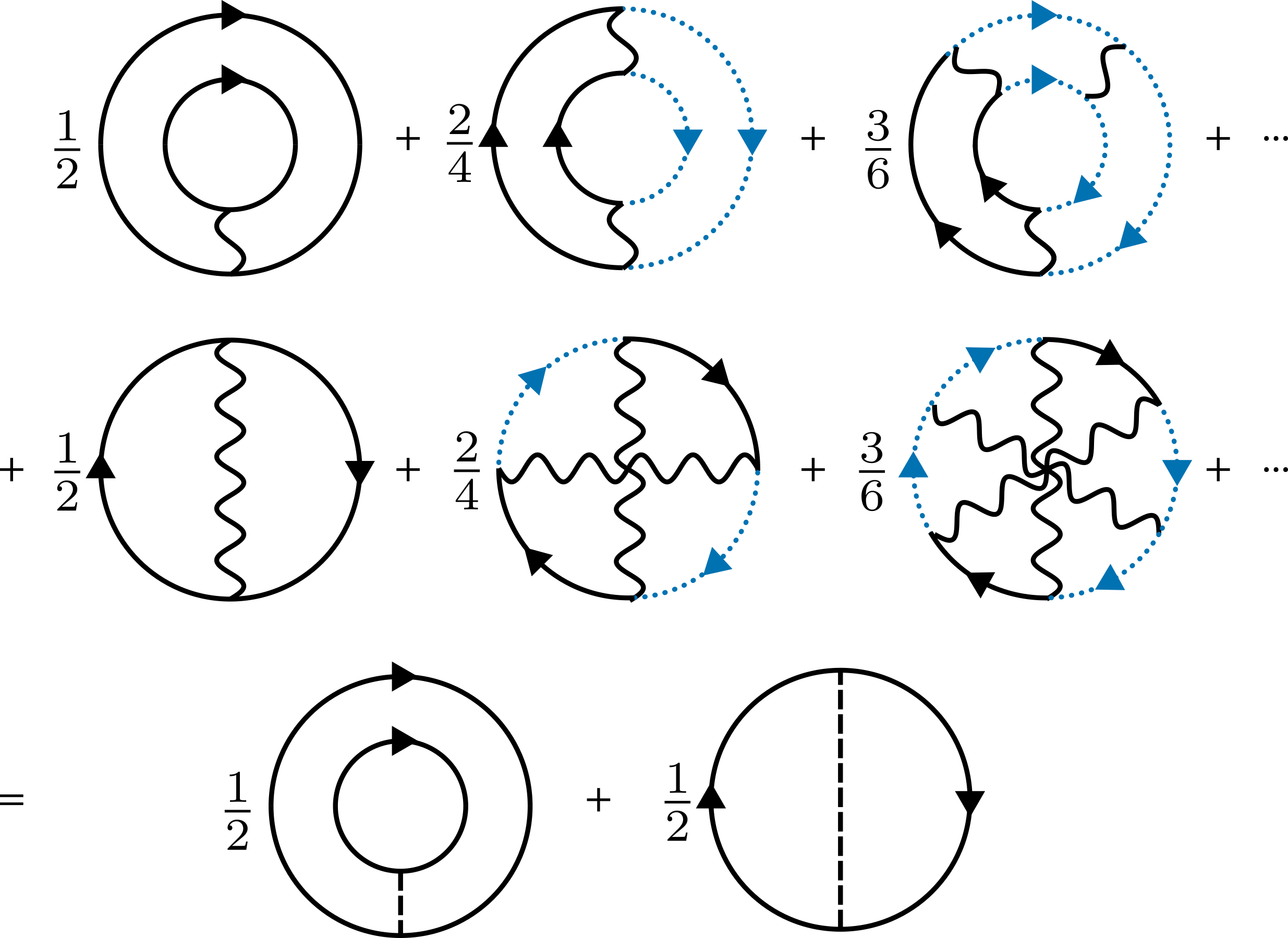
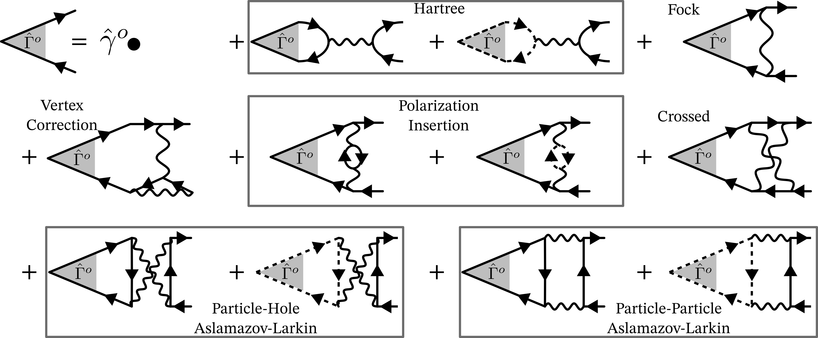
To establish the ground state, we need to obtain the energy as a function of the spin polarization. We will do so by computing the Luttinger-Ward functional within the same logarithmic approximation that we used for the susceptibility. The Luttinger-Ward functional containing the leading logarithmic terms at each order is shown in Fig. 7. Note that as is usual with LW approach, the Green’s function lines represent the full Green’s function , which must be solved for self-consistently 333The form of the variational Luttinger-Ward energy Eq. 4 guarantees that minimizing with respect to produces a self-consistent solution., and not the normal state Green’s function . The MF approximation Fig. 3 corresponds to keeping the first diagram in each of the two lines in Fig. 7.
Given the preceding discussion, the leading contribution to each diagram comes from when all but two pairs of particles are away from the Fermi surface, and the remaining particles are near the Fermi surface (see Fig. 8), as these terms come with the maximum logarithmic enhancement at each loop order. At this level, the combinatoric factors associated with ways of choosing out of lines to be near the Fermi surface in an loop diagram cancel the overall factor of , and the Luttinger-Ward functional retains the same form as in MF, Eq. 9, but with the effective interaction . In explicit form,
| (20) |
where is with respect to spin. However, as noted above, as long as the logarithmic approximation holds so there is no Stoner susceptibility within this regime.
II.5 Discussion
The general suppression of the Stoner susceptibility due to particle-particle ladders was discussed in the ’60s by Kanamori [37]. At a face value, Eq. 19 implies that there is no Stoner transition (using our designation of Stoner transition) in 2D. We caution, however, that it is entirely possible that a Stoner transition actually occurs but is pushed to larger values of where the logarithmic approximation breaks down. Mathematically, this corresponds to the fact that while at each order in , the ladder diagrams are largest, the series as a whole may not be absolutely convergent. Furthermore, there are systems for which it can be rigorously shown that a Stoner transition does occur, e.g., the half-filled Hubbard model on the Lieb lattice[40].
Given the uncertainty, we are left with the following three possibilities, which we already listed in the Introduction:
-
(I)
There is a transition of Stoner type, where the susceptibility diverges, outside the applicability of our resummation scheme,
-
(II)
There is a first-order transition to a polarized state with no divergence of the susceptibility,
-
(III)
There is no transition to a polarized state for any .
While that is all that can be theoretically said about the spin Stoner instability in a single-valley system within our treatment, we will see in the following sections that it is possible to make sharper predictions for a two-valley system.
III Two-valley system
We now consider how the story is modified in the presence of both spin and valley degrees of freedom. This is of particular interest for iso-spin instabilities in quasi-two-dimensional multi-valley systems such as BBG, RTG, and AlAs quantum wells.
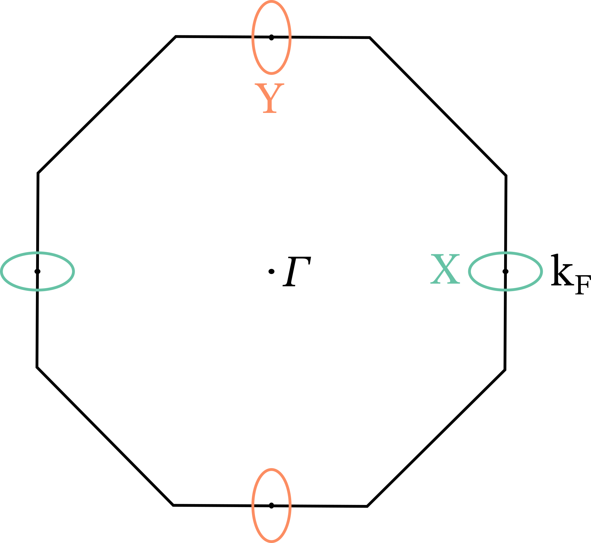
For definiteness, we consider a two-valley model appropriate for AlAs. The low-energy description of this system has all of the necessary components while remaining relatively simple. Bulk AlAs has a low-energy manifold consisting of ellipsoidal pockets near three inequivalent points in the Brillouin zone (three valleys). When confined along one of the periodic axes, e.g., , and placed atop a GaAs substrate, the energy spectrum splits between lower-energy excitations in the two in-plane and valleys (two pockets centered at , and ), and higher-energy excitations in the out-of-plane valley [18]. The 2D dispersion around and can be well approximated as quadratic with anisotropic band mass, leading to elliptical Fermi surfaces, see Fig. 9.
We follow [18, 19, 32, 33] and model the low-energy physics of AlAs by
| (21) |
where and are spin and valley degrees of freedom, respectively, and the valley dependent dispersion is
| (22) |
where the and valleys are centered, respectively, at the and points. The degree of anisotropy is set by the parameter . We will assume, without loss of generality, that , but all results are manifestly invariant with regard to .
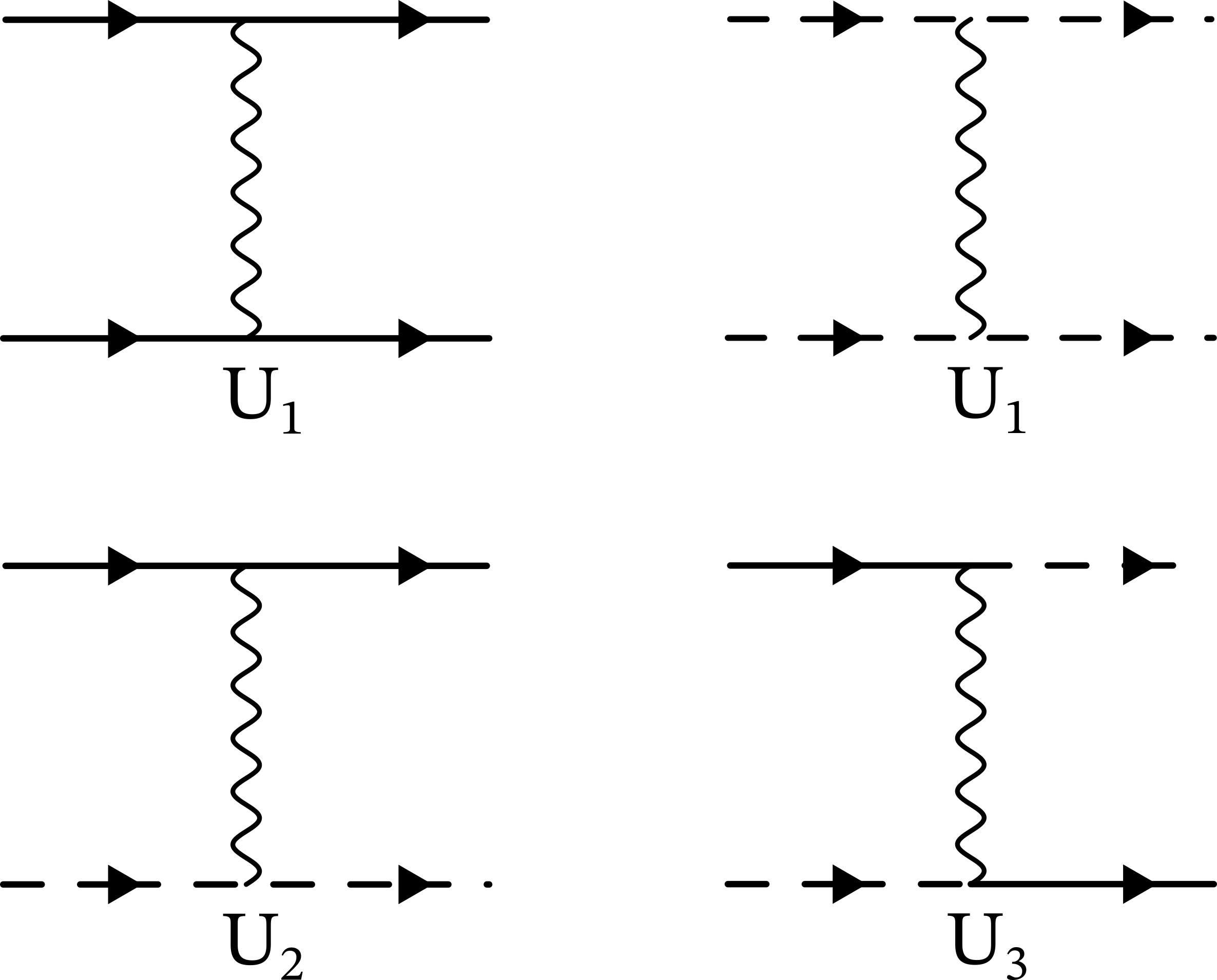
The interaction Hamiltonian consists of three short ranged interactions, depicted in Fig. 10: interaction between densities in the same valley , interaction between densities in different valleys , and scattering from one valley to another . All three interactions arise from the screened Coulomb interaction at the appropriate momentum, for and for . We consider the case where the Fermi momenta are much smaller than the separation between valleys , so that , and neglect 444As we will see later, it is important whether the Coulomb interaction is screened by the system itself our some other component of the setup, e.g., a nearby gate.. The interaction Hamiltonian then takes the form
| (23) |
III.1 Within MF
Five types of spin/valley order can develop in this model within the MF approximation [25, 31]. They are one-component valley-polarization (VP) (), three-component ferromagnetism (FM) (), three-component staggered ferromagnetism (SFM) (), two-component inter-valley coherence (IVC) (), and six-component spin inter-valley coherence (sIVC) (). For and , the model is SU(4) symmetric and the MF susceptibilities for all orders are identical. Analogous to the calculation of Sec. II we find
| (24) |
The MF ground state energy of SU(4)-symmetric model can be compactly written in a form similar to Eq. 10:
| (25) |
with the energy of the normal state. However, the energy is now parametrized by three polarizations as there are four iso-spin bands 555 The polarizations are also subject to additional constraints arising from conservation of the total density. See 35, *Raines2024b for details on the parameterization. . At , the energy is minimized by making the largest possible, hence there is again a strong first-order transition accompanied by the divergence of susceptibility at approaching from below. The resulting state is a highly degenerate quarter-metal state, with 3 spontaneously depopulated bands and one band containing all fermions (see [35, *Raines2024b] for details).
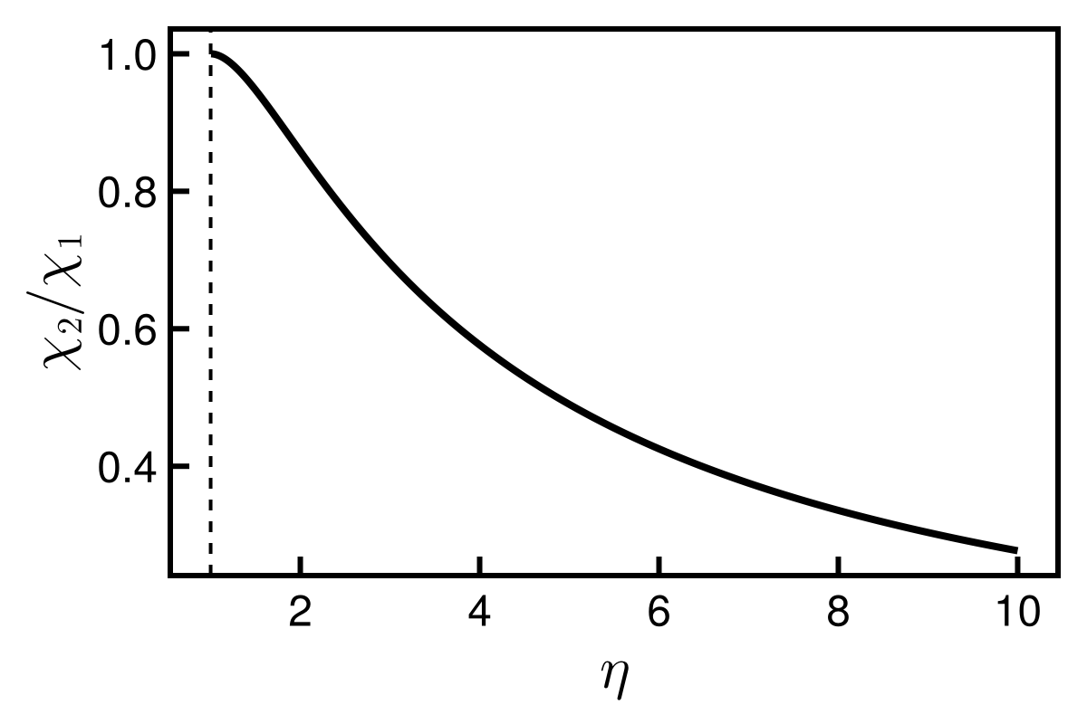
For finite anisotropy () the degeneracy is partly lifted, with IVC and sIVC states becoming energetically disfavored. This can be seen by comparing the bare static susceptibilities in each channel; these now take different values depending on whether the associated order is at small momentum (VP, FM, SFM) or large momentum (IVC, sIVC). Concretely , and with
| (26) |
At these evaluate to
| (27) |
The ratio is a decreasing function of (see Fig. 11) and thus anisotropy favors zero momentum states, i.e., VP, FM, and SFM orders. These three, however, remain degenerate as long as , and there is still a first-order transition to a quarter-metal state (three empty bands and one filled band) at , where VP, FM and SFM susceptibilities diverge. The only difference with the SU(4) case is the number of Goldstone modes in the quarter-metal state.
When , FM and SFM orders are still degenerate, but the degeneracy between VP and FM/SFM is lost. To obtain dressed VP and FM/SFM susceptibilities we can again calculate the renormalized vertices
| (28) |
where VP, FM/SFM, , and . At the mean-field level the vertices obey a one-loop Bethe-Salpeter equation of the form
| (29) |
where and denote Hartree and Fock contributions, specified in Fig. 12. The matrix structure of the vertices is not changed by renormalization, hence , where
| (30) |
and the susceptibility is related to by
| (31) |
The Fock diagram is identical for the VP and FM/SFM channels:
| (32) |
Here is the normal state matrix Green’s function with spin and valley indices, i.e.,
| (33) |
The two Hartree diagrams, on the other hand, are non-zero only for the VP channel:
| (34) |
while . Plugging these into the right hand side of Eq. 30 we obtain the MF result for the renormalized vertices:
| (35) |
For , FM/SFM order develops first, while for , VP order develops first. In each case, there is sequence of first-order transitions: first into a half-metal state and then into a quarter metal state. Near each transition, the corresponding susceptibility diverges. The mean field approximation to the Luttinger-Ward functional is shown in Fig. 3, where now solid fermionic lines represent the full matrix Green’s functions with both spin and valley indices, and the wavy line represents the bare Hubbard interactions and with appropriate matrix structure in valley space (cf. Eq. 23). In analytical form,
| (36) |
where the trace is now over both spin and valley and are raising (lowering) Pauli matrices in valley space. Minimizing Eq. 4 with respect to one obtains the mean-field Green’s function and the mean-field ground state energy Eq. 25, from .
III.2 Iso-spin susceptibility beyond MF
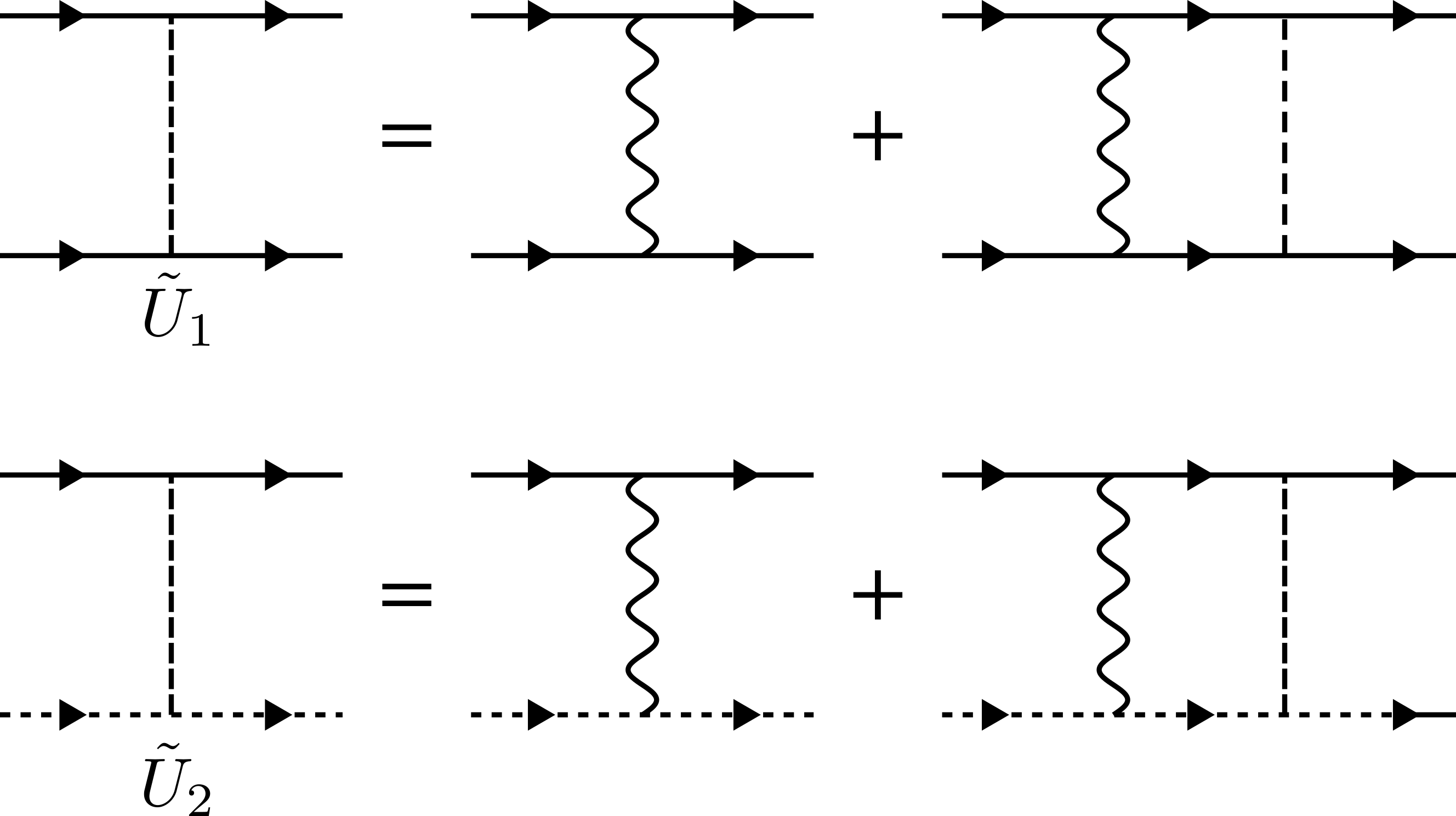
We now turn to the question of how the FM/SFM and VP instabilities are modified beyond the MF approximation. As before, we start by considering the Bethe-Salpeter equation in VP and FM/SFM channels with two-loop diagrams for the irreducible four-point function. We will see that in the low density limit certain diagrams are enhanced by . The two-loop contributions to the Bethe-Salpeter equation are shown in the second and third lines of Fig. 12. They include the corrections to the side vertices in the one-loop Fock diagram, the term with inserted particle-hole polarization, the diagram with crossed interaction lines, and two types of Aslamazov-Larkin (AL) diagrams with parallel and crossed interaction lines. We verified that logarithmic renormalizations come from the diagrams with crossed interaction lines, which contain particle-particle polarization bubble with unconstrained momentum integration. For definiteness, we call the last diagram in the second line in Fig. 12 the crossed diagram and the last two in the third line AL particle-particle diagrams. In other diagrams, all intermediate fermions are constrained to be near the Fermi surface. As a consequence, to logarithmic accuracy, we need only keep the crossed diagram and the particle-particle AL diagrams. The calculation of the crossed diagram proceeds as for the spin-only case, Eq. 12, with the only difference being a factor of due to the extra degrees of freedom in the spin and valley model. This diagram does not distinguish between VP and FM/SFM vertices and gives
| (37) |
where is the external momentum/frequency, and . There is no summation over and the result is the same for and . One can easily verify that integration over is constrained to the Fermi surface, but integration over is not constrained, and that the logarithmic contribution comes from . For these , can be approximated by
| (38) |
where we used . Notice that the anisotropy does not enter as it does not affect the density of states in each valley. In contrast, the AL particle-particle diagrams distinguish between VP and FM/SFM vertices. For the latter, these diagrams vanish due to the spin summation, i.e., Eq. 38 is the only contribution at the two-loop order. Solving the BS equation in the FM/SFM channels we obtain, at the two-loop level,
| (39) |
Clearly, the two-loop crossed diagram suppresses the tendency towards a Stoner instability in the FM and SFM channels.
For the VP vertex, the particle-particle AL term does not vanish and is given by
| (40) |
where we have performed a rotation in the second term to simplify the expression. The logarithmic contribution again comes from internal momenta , when the integration in Eq. 40 factorizes to
| (41) |
where we have defined
| (42) |
For the former, we have, similar to the crossed diagram,
| (43) |
On the other hand, involves particles at both valleys and thus depends on the anisotropy. Evaluating this contribution we find (see Appendix B)
| (44) |
Putting together crossed and AL contributions, we obtain
| (45) |
Adding the one-loop term we obtain the two-loop expression for the VP vertex
| (46) |
Comparing Eqs. 39 and 46, we see that the two-loop renormalizations of the VP and FM/SFM vertices are different even if we set . In this last case,
| (47) |
Notice that for , the logarithmic suppression is weaker in the VP channel than in the FM/SFM channels. Furthermore, for , the two-loop renormalization of actually increases the tendency towards the Stoner instability.
As we did for the spin-only case, we next go beyond two-loop order. To simplify the presentation, we set . As before, note that at -loop order, maximally crossed irreducible diagrams come with a factor of due to factors of , while any other diagrams have lower powers of . Evaluating the irreducible vertices with logarithmic accuracy by keeping the diagrams with the largest power of at each loop order, and solving then Bethe-Salpeter equations for , we obtain
| (48) |
which formally look the same as in MF approximation, but with the effective interactions
| (49) |
The corresponding susceptibilities are
| (50) |
In Ref. [33] the same and have been obtained by summing ladder series of particle-particle diagrams for the renormalized interactions (see Fig. 13).
III.3 Ground state energy beyond MF
To obtain the ground state, we employ the Luttinger-Ward functional as we did for the spin-only case, Sec. II.4. Specifically we sum the logarithmically enhanced terms in Fig. 7, where solid fermionic lines now represent matrix Green’s functions with both spin and valley indices, and the interaction lines include both intra- and inter-valley interactions and . Recall that the MF approximation Fig. 3 corresponds to keeping the first diagram in each of the two lines in Fig. 7.
Again, the leading contribution to each diagram comes from when all but two pairs of particles are away from the Fermi surface, and the remaining particles are near the Fermi surface, Fig. 8, so the combinatoric factors associated with ways of choosing out of lines to be near the Fermi surface in an loop diagram cancel the overall factor of . Therefore, like in the spin-only case, the Luttinger-Ward functional retains the same form as in MF, Eq. 36, but with the effective interactions and . In explicit form,
| (51) |
The outcome of this analysis is the following:
-
1.
The MF-like description of the Stoner transition in a two-valley system remains valid once we include leading logarithmic renormalizations beyond MF, but with the original interactions and renormalized to effective interactions and .
-
2.
For a circular Fermi surface, both and are strongly reduced compared to the original interactions such that as long as the theory remains under control, the condition for a Stoner instability in any channel is not satisfied. Whether the instability develops at even larger is beyond the scope of this paper.
-
3.
For an elliptical Fermi surface in each valley, governed by , is still strongly reduced, but is reduced less. In the limit of strong anisotropy, .
-
4.
As a consequence, Stoner transitions into FM and SFM states do not occur within the logarithmic approximation, but a Stoner transition into the VP state does occur if the anisotropy is strong enough.
-
5.
For , the Stoner instability towards VP occurs at smaller than at the mean field level ().
-
6.
The VP susceptibility diverges upon approaching the Stoner instability from below, and is zero on the other side of the transition where the VP order parameter jumps to its maximum value. The same happens near a FM/SFM transition if we treat as a parameter which can reach
This last item is the most remarkable outcome of the current treatment: the unconventional nature of Stoner transitions in 2D is preserved in the logarithmic approximation beyond MF. Namely, the transitions are strongly first order into maximally ordered states, yet the corresponding susceptibility diverges as the system approaches an instability from the disordered side.
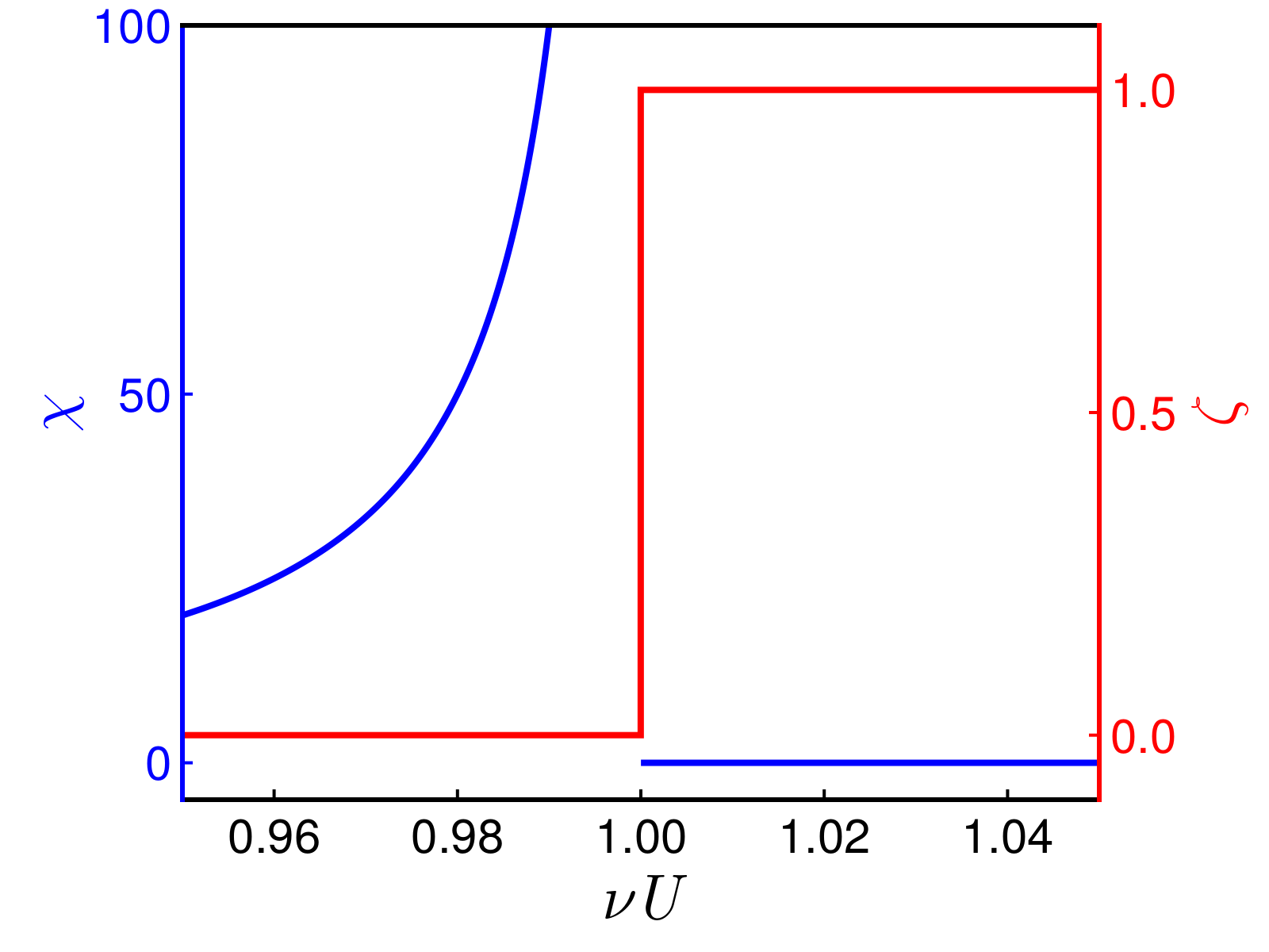
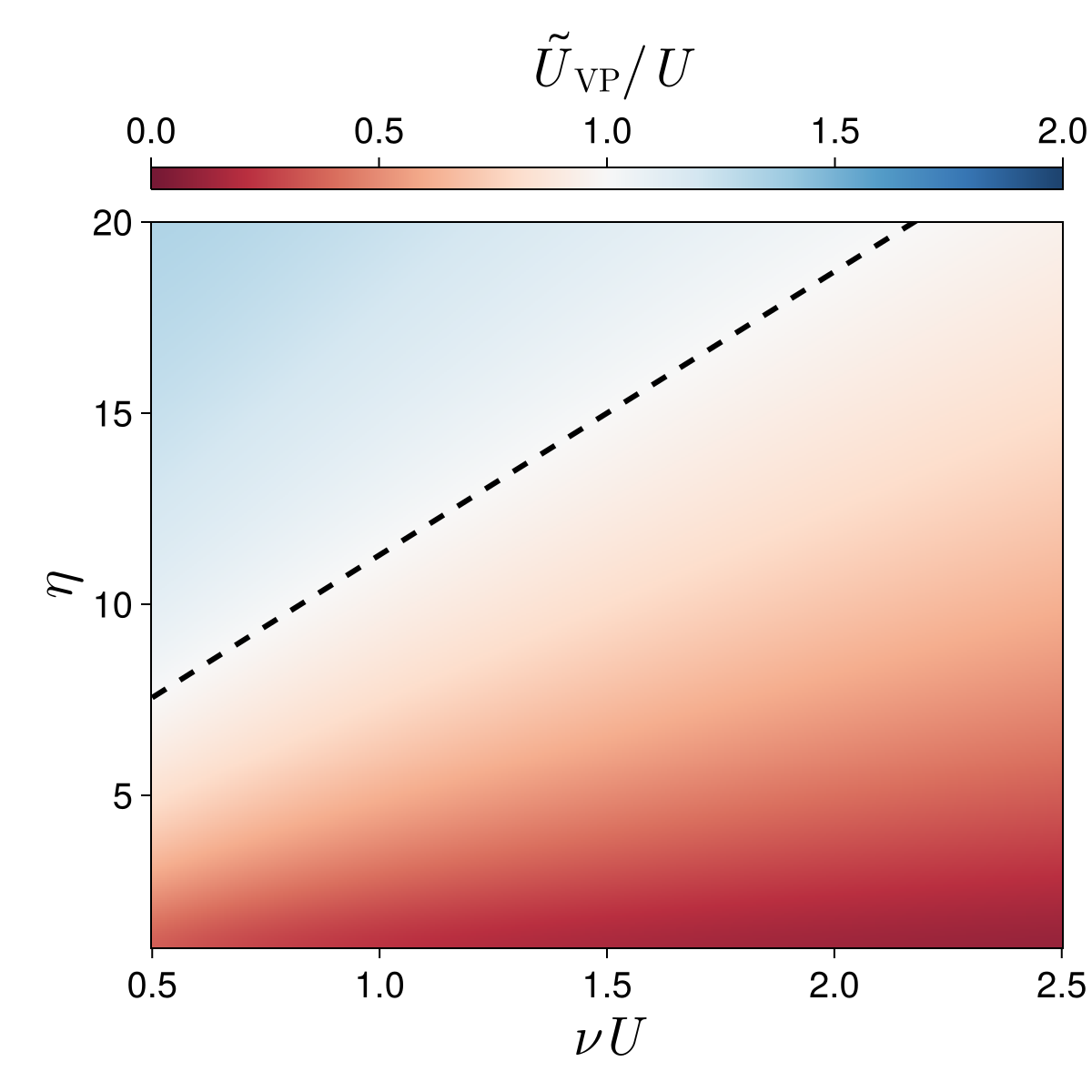
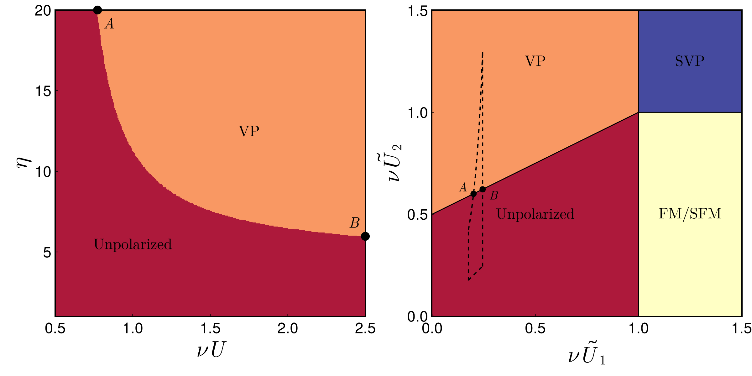
In Fig. 14 we plot the effective vs the bare interaction in the VP channel, , which is when . At large , the condition is reached at smaller than the condition , i.e., the Stoner transition into the VP state occurs at smaller than in MF. In Fig. 15 we present the phase diagrams. The left panel is the phase diagram obtained within our logarithmic approximation. A FM/SFM order does not develop, but VP order develops and the critical get reduced as increases. The right panel is the formal phase diagram obtained by treating and as variables. The region inside the dashed lines is the one in the left panel.
IV Comparison with RPA
It is worth comparing our conclusions with those obtained in Ref. [33] for the Coulomb interaction treated within the RPA. The RPA approximation to the energy employed therein amounts to summing all ring diagrams of particle-hole bubbles. We, on the contrary, estimated the Luttinger-Ward functional as a series of particle-particle bubbles in the full Green’s function, corresponding to keeping only the largest contribution at each loop-order. There are some differences in these approaches due to directly using the diagrammatic expansion of the energy vs. the Luttinger-Ward formalism, which we cover in Sec. IV.1, but we first discuss the primary differences which arise due to the summation of particle-particle vs. particle-hole bubbles and the implications for experiments in AlAs.
Minimizing the RPA ground state energy, the authors of [33] obtained the phase diagram as function of and . By increasing at large enough , they found a first-order transition into the VP state and then another first-order transition into spin and valley-polarized state (SVP). The critical for the VP decreases as increases. These results are in line with earlier variational Quantum Monte Carlo calculation by the same group [32].
The sequence of ordered states and the reduction of the critical interaction for VP for larger are consistent with our results. However, the VP and FM/SFM susceptibilities obtained in [33] do not display a Stoner-like divergence. The difference comes from the fact that the RPA is an infinite series in particle-hole bubbles, while in our calculation we included an infinite series in particle-particle bubbles. At second order, both approaches include the second diagram in Fig. 7, which introduces a difference between VP and FM/SFM order, and hence we all found that the tendency towards VP is stronger. But higher-loop diagrams are different in their and our approaches. Unlike our case, there is no cancellation of the diagrammatic combinatoric factors in the RPA, and hence there is no particular relationship between the condition for the first-order transition and the behavior of the susceptibility at the transition point.
That the susceptibilities do not diverge within RPA can be qualitatively understood by noticing that the RPA screened Coulomb interaction is
| (52) |
where and the factor of comes from the spin and valley sums. The screened Coulomb interaction never approaches the point , where the susceptibility would diverge.
On physical grounds, it is crucial to our considerations that the cutoff scale of the interaction be large compared to the Fermi momentum. For the Hubbard-like model we consider is of order the Brillouin zone size. In this situation, if is far smaller than , our treatment involves keeping only the largest terms at each order, while the terms included in the RPA are of order , i.e., are smaller. However, for systems where the interaction is more long-ranged, the cutoff scale could be instead related to a property of the interaction itself. In particular, the authors of [33] argued that if is related to the screening gate separation, it may be comparable to , and is no longer a large parameter. In this situation, particle-hole diagrams can no longer be neglected, but contributions from the particle-particle channel cannot be neglected either.
IV.1 Self-consistency: Conserving vs. Non-conserving
One other difference between the approach employed in [33] and this work relates to self-consistent nature of the Luttinger-Ward calculation, and correspondingly the lack of self-consistency in the RPA calculation. Note, that in general including the particle-hole ring diagrams in the Luttinger-Ward functional is different from evaluating the diagrams of the same type in the RPA approach (Ref. [33]). Within the Luttinger-Ward formalism the Green’s function is to be calculated fully self-consistently. The RPA summation on the other hand uses a free-fermion-like ansatz for the Green’s function with an iso-spin dependent chemical potential.
As noted in Sec. II.2, for the Hubbard model the distinction does not matter for either the MF or logarithmic approximations, as the self-energy obtained from the Luttinger-Ward functional is constant. Thus, the Green’s function is of free-fermion-like form and it does not matter where we use the Luttinger-Ward functional or calculate the energy directly from the variational Green’s function.
On the other hand, if one considers the Luttinger-Ward functional obtained from summing ring diagrams, sometimes called the self-consistent GW approximation, the self-energy is in general a function of frequency and momentum. The RPA summation scheme thus differs in that the self-energy equation is not evaluated self-consistently (this is sometimes called the approximation). For this reason, the RPA is in principle not a fully self-consistent conserving approximation as opposed to calculations within the Luttinger-Ward functional. Of course, self-consistency does not guarantee the best approximation.
IV.2 Application to AlAs
The phase diagram of AlAs quantum wells as a function of electron density has been thoroughly investigated in recent years [34, 18, 19, 20, 21]. As mentioned in Sec. III bulk AlAs has ellipsoidal Fermi pockets near the three inequivalent points in the Brillouin zone. When confined along one of the periodic axes, e.g. , and placed atop a GaAs substrate, the energy spectrum splits between lower-energy excitations in the two in-plane and valleys and higher-energy excitations in the out-of-plane valley [18]. When the Fermi level is placed in valleys, the low-energy excitations are located in the and valleys, near elliptical Fermi pockets centered at , and and related by a rotation which exchanges the and points.
Resistivity measurements in the presence of an external strain and magnetic field reveal two ordered states that appear upon decreasing electron density, i.e., upon increasing . At the first critical , the system undergoes a strong first-order transition into a VP state, at which one of the valleys moves above the Fermi level (a half-metal state). Then, at , there is another first-order transition into SVP state, when the spins in the remaining valley order ferromagnetically and the band with one spin projection moves above the Fermi level (a quarter-metal state). The experimentally observed sequence of transitions into VP and then SVP states has been reproduced in variational Monte Carlo calculations for a two-valley system with elliptical Fermi surfaces and Coulomb interaction [32], although at smaller than in the experiments. These studies also found that the critical for the VP transition gets smaller with increasing ellipticity of the Fermi surfaces, i.e., with increasing . A similar phase diagram holds also for the Hubbard interaction [49]
The sequence of first-order transitions, the disappearance of some of Fermi surfaces immediately above the transition, and the reduction of the threshold for VP with increasing is consistent with our results and with the RPA calculations in Ref. [33]. The distinguishing feature of our theory is the prediction that the transitions remain Stoner-like, i.e., that the VP and spin susceptibilities diverge upon approaching the corresponding transitions from a disordered side. We emphasize that this holds in the logarithmic approximation that we used. Beyond this approximation, when RPA-type corrections to the Luttinger-Ward functional (ring diagrams) are included, the susceptibility saturates at a finite value at each transition. However, if is sizable, our theory predicts that the susceptibilities should still be substantially enhanced near the VP and FM transitions.
In Refs. [34, 18, 20], the authors where able to measure the valley susceptibility in AlAs with high precision. The experiments measured the valley occupation as a function of strain, which acted as a valley dependent potential, using two complementary methods. One method relies on the anisotropic nature of the and Fermi pockets, allowing the resistivities , along the and directions, respectively, act as a direct proxy for the densities in the corresponding valleys. The other obtained the valley densities from the characteristic frequencies of Shubnikov-de Haas oscillations In either case, the VP susceptibility can then be obtained as, . Both methods found, with good agreement, that the valley susceptibility grows as the density decreases, corresponding to larger , but the susceptibility in the immediate vicinity of critical was not measured.
Additionally, the authors of [19] extracted the spin susceptibility from their experimental measurements of magnetoresistance near the subsequent spin transition and argued that it strongly (by more than an order of magnitude) increases as the transition is approached. While this regime is inaccessible within our approach, this behavior is in line with the prediction that within logarithmic approximation both transitions remain Stoner-like with the same behavior as in MF.
V Discussion and Conclusion
In this paper, we analyzed the iso-spin instabilities of a low-density 2D Fermi gas beyond MF theory. We showed that particle-particle ladder renormalization of the interactions are parametrically the largest contribution in the large parameter . For an isotropic system this leads to a suppression of the interaction strength such that and Stoner instabilities cannot occur within the regime of applicability of this approximation. It should, however, be emphasized that this does not preclude the occurrence of itinerant ferromagnet — indeed it has been proven that such states occur on e.g., the Lieb lattice [40] — but rather that the instability must occur outside the regime of applicability of the logarithmic approximation.
When anisotropy is introduced in the form of a valley-dependent Fermi surface distortion, we showed that the renormalizations uniquely favor a valley polarization order, which for large enough anisotropy can develop within the logarithmic approximation. Interestingly, the unconventional features of the MF instability persist — namely, the VP transition is first-order into a half-metal state, with one valley completely depopulated, and the valley iso-spin susceptibility diverges as the transition point is approached from the unpolarized state. Thus, a first-order Stoner transition is not an artifact of MF theory and, at least in some parameter regimes, remains when beyond MF corrections are included. A first order transition into a VP state with a growing VP susceptibility has been observed experimentally in AlAs [20].
Acknowledgements.
We thank A.A. Allocca, C. Batista, E. Berg, L. Glazman, S. Huber, S. Kivelson, L. Levitov, D. Maslov, J.H. Wilson and particularly M. Randeria for fruitful discussions and feedback. The work was supported by the U.S. Department of Energy, Office of Science, Basic Energy Sciences, under Award No. DE-SC0014402 and by the Fine Theoretical Physics Institute at the University of Minnesota.References
- Bistritzer and MacDonald [2010] R. Bistritzer and A. H. MacDonald, Transport between twisted graphene layers, Physical Review B 81, 245412 (2010).
- Schaibley et al. [2016] J. R. Schaibley, H. Yu, G. Clark, P. Rivera, J. S. Ross, K. L. Seyler, W. Yao, and X. Xu, Valleytronics in 2D materials, Nature Reviews Materials 1, 10.1038/natrevmats.2016.55 (2016).
- Žutić et al. [2004] I. Žutić, J. Fabian, and S. Das Sarma, Spintronics: Fundamentals and applications, Reviews of modern physics 76, 323 (2004).
- Cao et al. [2018a] Y. Cao, V. Fatemi, A. Demir, S. Fang, S. L. Tomarken, J. Y. Luo, J. D. Sanchez-Yamagishi, K. Watanabe, T. Taniguchi, E. Kaxiras, R. C. Ashoori, and P. Jarillo-Herrero, Correlated insulator behaviour at half-filling in magic-angle graphene superlattices, Nature 556, 80 (2018a).
- Cao et al. [2018b] Y. Cao, V. Fatemi, S. Fang, K. Watanabe, T. Taniguchi, E. Kaxiras, and P. Jarillo-Herrero, Unconventional superconductivity in magic-angle graphene superlattices, Nature 556, 43 (2018b).
- Andrei and MacDonald [2020] E. Y. Andrei and A. H. MacDonald, Graphene bilayers with a twist, Nature Materials 19, 1265 (2020).
- Hu et al. [2023] H. Hu, B. A. Bernevig, and A. M. Tsvelik, Kondo lattice model of magic-angle twisted-bilayer graphene: Hund’s rule, local-moment fluctuations, and low-energy effective theory, Physical Review Letters 131, 026502 (2023).
- Seiler et al. [2022] A. M. Seiler, F. R. Geisenhof, F. Winterer, K. Watanabe, T. Taniguchi, T. Xu, F. Zhang, and R. T. Weitz, Quantum cascade of correlated phases in trigonally warped bilayer graphene, Nature 608, 298 (2022).
- Zhou et al. [2022] H. Zhou, L. Holleis, Y. Saito, L. Cohen, W. Huynh, C. L. Patterson, F. Yang, T. Taniguchi, K. Watanabe, and A. F. Young, Isospin magnetism and spin-polarized superconductivity in Bernal bilayer graphene, Science 375, 774 (2022).
- Zhou et al. [2021] H. Zhou, T. Xie, A. Ghazaryan, T. Holder, J. R. Ehrets, E. M. Spanton, T. Taniguchi, K. Watanabe, E. Berg, M. Serbyn, et al., Half-and quarter-metals in rhombohedral trilayer graphene, Nature 598, 429 (2021).
- de la Barrera et al. [2022] S. C. de la Barrera, S. Aronson, Z. Zheng, K. Watanabe, T. Taniguchi, Q. Ma, P. Jarillo-Herrero, and R. Ashoori, Cascade of isospin phase transitions in Bernal bilayer graphene at zero magnetic field, Nature Physics 18, 771 (2022), arXiv:2110.13907 [cond-mat] .
- Seiler et al. [2024] A. M. Seiler, M. Statz, I. Weimer, N. Jacobsen, K. Watanabe, T. Taniguchi, Z. Dong, L. S. Levitov, and R. T. Weitz, Interaction-Driven Quasi-Insulating Ground States of Gapped Electron-Doped Bilayer Graphene, Physical Review Letters 133, 066301 (2024), arXiv:2308.00827 [cond-mat.str-el] .
- Arp et al. [2024] T. Arp, O. Sheekey, H. Zhou, C. L. Tschirhart, C. L. Patterson, H. M. Yoo, L. Holleis, E. Redekop, G. Babikyan, T. Xie, J. Xiao, Y. Vituri, T. Holder, T. Taniguchi, K. Watanabe, M. E. Huber, E. Berg, and A. F. Young, Intervalley coherence and intrinsic spin–orbit coupling in rhombohedral trilayer graphene, Nature Physics 10.1038/s41567-024-02560-7 (2024), arXiv:2310.03781 [cond-mat.mes-hall] .
- Holleis et al. [2023] L. Holleis, C. L. Patterson, Y. Zhang, H. M. Yoo, H. Zhou, T. Taniguchi, K. Watanabe, S. Nadj-Perge, and A. F. Young, Ising Superconductivity and Nematicity in Bernal Bilayer Graphene with Strong Spin Orbit Coupling (2023), arXiv:2303.00742 [cond-mat.supr-con] .
- Zhang et al. [2023] Y. Zhang, R. Polski, A. Thomson, É. Lantagne-Hurtubise, C. Lewandowski, H. Zhou, K. Watanabe, T. Taniguchi, J. Alicea, and S. Nadj-Perge, Enhanced superconductivity in spin–orbit proximitized bilayer graphene, Nature 613, 268 (2023).
- Huang et al. [2023] C. Huang, T. M. R. Wolf, W. Qin, N. Wei, I. V. Blinov, and A. H. MacDonald, Spin and orbital metallic magnetism in rhombohedral trilayer graphene, Physical Review B 107, L121405 (2023).
- Blinov et al. [2023] I. V. Blinov, C. Huang, N. Wei, Q. Wei, T. Wolf, and A. H. MacDonald, Partial condensation of mobile excitons in graphene multilayers (2023), arXiv:2303.17350 [cond-mat.mes-hall] .
- Shayegan et al. [2006] M. Shayegan, E. P. De Poortere, O. Gunawan, Y. P. Shkolnikov, E. Tutuc, and K. Vakili, Two-dimensional electrons occupying multiple valleys in AlAs, physica status solidi (b) 243, 3629 (2006).
- Hossain et al. [2020] M. S. Hossain, M. K. Ma, K. A. V. Rosales, Y. J. Chung, L. N. Pfeiffer, K. W. West, K. W. Baldwin, and M. Shayegan, Observation of spontaneous ferromagnetism in a two-dimensional electron system, Proceedings of the National Academy of Sciences 117, 32244 (2020).
- Hossain et al. [2021] Md. S. Hossain, M. K. Ma, K. A. Villegas-Rosales, Y. J. Chung, L. N. Pfeiffer, K. W. West, K. W. Baldwin, and M. Shayegan, Spontaneous valley polarization of itinerant electrons, Physical Review Letters 127, 116601 (2021).
- Hossain et al. [2022] Md. S. Hossain, M. K. Ma, K. A. Villegas-Rosales, Y. J. Chung, L. N. Pfeiffer, K. W. West, K. W. Baldwin, and M. Shayegan, Anisotropic two-dimensional disordered wigner solid, Physical Review Letters 129, 036601 (2022).
- Ghazaryan et al. [2021] A. Ghazaryan, T. Holder, M. Serbyn, and E. Berg, Unconventional superconductivity in systems with annular fermi surfaces: Application to rhombohedral trilayer graphene, Physical Review Letters 127, 247001 (2021).
- Chatterjee et al. [2022] S. Chatterjee, T. Wang, E. Berg, and M. P. Zaletel, Inter-valley coherent order and isospin fluctuation mediated superconductivity in rhombohedral trilayer graphene, Nature Communications 13, 6013 (2022).
- Chichinadze et al. [2022a] D. V. Chichinadze, L. Classen, Y. Wang, and A. V. Chubukov, Cascade of transitions in twisted and non-twisted graphene layers within the van Hove scenario, npj Quantum Materials 7, 114 (2022a).
- Chichinadze et al. [2022b] D. V. Chichinadze, L. Classen, Y. Wang, and A. V. Chubukov, SU(4) Symmetry in Twisted Bilayer Graphene: An Itinerant Perspective, Physical Review Letters 128, 227601 (2022b).
- You and Vishwanath [2022] Y.-Z. You and A. Vishwanath, Kohn-Luttinger superconductivity and intervalley coherence in rhombohedral trilayer graphene, Physical Review B 105, 134524 (2022).
- Szabó and Roy [2022] A. L. Szabó and B. Roy, Competing orders and cascade of degeneracy lifting in doped Bernal bilayer graphene, Physical Review B 105, L201107 (2022).
- Zang et al. [2022] J. Zang, J. Wang, J. Cano, A. Georges, and A. J. Millis, Dynamical Mean-Field Theory of Moiré Bilayer Transition Metal Dichalcogenides: Phase Diagram, Resistivity, and Quantum Criticality, Physical Review X 12, 021064 (2022).
- Xie and Das Sarma [2023] M. Xie and S. Das Sarma, Flavor symmetry breaking in spin-orbit coupled bilayer graphene, Physical Review B 107, L201119 (2023).
- Dong et al. [2023a] Z. Dong, M. Davydova, O. Ogunnaike, and L. Levitov, Isospin- and momentum-polarized orders in bilayer graphene, Physical Review B 107, 075108 (2023a).
- Dong et al. [2023b] Z. Dong, O. Ogunnaike, and L. Levitov, Collective Excitations in Chiral Stoner Magnets, Physical Review Letters 130, 206701 (2023b).
- Valenti et al. [2024] A. Valenti, V. Calvera, S. A. Kivelson, E. Berg, and S. D. Huber, Nematic Metal in a Multivalley Electron Gas: Variational Monte Carlo Analysis and Application to AlAs, Physical Review Letters 132, 266501 (2024), arXiv:2307.15119 [cond-mat.str-el] .
- Calvera et al. [2024] V. Calvera, A. Valenti, S. D. Huber, E. Berg, and S. A. Kivelson, Theory of Coulomb driven nematicity in a multi-valley two-dimensional electron gas (2024), arXiv:2406.12825 [cond-mat] .
- Gunawan et al. [2006] O. Gunawan, Y. P. Shkolnikov, K. Vakili, T. Gokmen, E. P. De Poortere, and M. Shayegan, Valley Susceptibility of an Interacting Two-Dimensional Electron System, Physical Review Letters 97, 186404 (2006).
- Raines et al. [2024a] Z. M. Raines, L. I. Glazman, and A. V. Chubukov, Unconventional discontinuous transitions in a 2D system with spin and valley degrees of freedom (2024a), arXiv:2406.04416 [cond-mat] .
- Raines et al. [2024b] Z. M. Raines, L. I. Glazman, and A. V. Chubukov, Unconventional discontinuous transitions in isospin systems (2024b), arXiv:2406.04415 [cond-mat] .
- Kanamori [1963] J. Kanamori, Electron Correlation and Ferromagnetism of Transition Metals, Progress of Theoretical Physics 30, 275 (1963).
- Irkhin et al. [2001] V. Yu. Irkhin, A. A. Katanin, and M. I. Katsnelson, Effects of van Hove singularities on magnetism and superconductivity in the t - t Hubbard model: A parquet approach, Physical Review B 64, 165107 (2001).
- Ojajärvi et al. [2024] R. Ojajärvi, A. V. Chubukov, Y.-C. Lee, M. Garst, and J. Schmalian, Pairing at a single Van Hove point (2024), arXiv:2408.05572 [cond-mat] .
- Lieb [1989] E. H. Lieb, Two theorems on the Hubbard model, Physical Review Letters 62, 1201 (1989).
- Abanov and Chubukov [2020] A. Abanov and A. V. Chubukov, Interplay between superconductivity and non-Fermi liquid at a quantum critical point in a metal. I. The model and its phase diagram at T = 0 : The case 0 1, Physical Review B 102, 024524 (2020).
- Hauck et al. [2020] D. Hauck, M. J. Klug, I. Esterlis, and J. Schmalian, Eliashberg equations for an electron–phonon version of the Sachdev–Ye–Kitaev model: Pair breaking in non-Fermi liquid superconductors, Annals of Physics , 168120 (2020).
- Luttinger and Ward [1960] J. M. Luttinger and J. C. Ward, Ground-State Energy of a Many-Fermion System. II, Physical Review 118, 1417 (1960).
- Baym and Kadanoff [1961] G. Baym and L. P. Kadanoff, Conservation Laws and Correlation Functions, Physical Review 124, 287 (1961).
- Baym [1962] G. Baym, Self-Consistent Approximations in Many-Body Systems, Physical Review 127, 1391 (1962).
- Lifšic et al. [2006] E. M. Lifšic, L. P. Pitaevskij, L. D. Landau, and E. M. Lifshitz, Statistical Physics. Part 2. Theory of the Condensed State, reprinted ed., Course of Theoretical Physics, Vol. 9 (Elsevier, Oxford, 2006).
- Galitskii [1958] VM. Galitskii, The energy spectrum of a non-ideal Fermi gas, Soviet Physics–JETP [translation of Zhurnal Eksperimentalnoi i Teoreticheskoi Fiziki] 7, 104 (1958).
- Fetter and Walecka [2012] A. L. Fetter and J. D. Walecka, Quantum Theory of Many-Particle Systems (Courier Corporation, 2012).
- Berg [2024] E. Berg, Private Communication (2024).
Appendix A Intra- and Inter-band susceptibilities
In this section, we present the details of the calculation of the susceptibilities in Eq. 27 at .
For the intra-band susceptibility we have
| (53) |
The inter-band case requires more work. First taking the limit we have
| (54) |
Defining and , and dividing the angular integration into identical regions we can write
| (55) |
Taking the derivative of the integral with respect to
| (56) |
where in the last line we made the change of variables in the second term. The integration is now elementary
| (57) |
Appendix B Intra- and Inter-valley particle-particle bubbles
The evaluation of the particle-particle bubbles for the two valley case is qualitatively similar to the spin-only case. We wish to evaluate the intra-valley bubble and inter-valley bubble :
| (58) |
For the former, we have, similar to the crossed diagram,
| (59) |
where the extra factor of comes from the spin degree of a freedom. Notice that the anisotropy does not enter as it does not affect the density of states. On the other hand, involves particles at both valleys and thus depends on the anisotropy. Defining
| (60) |
We can neglect the factor of in the denominator since the energy of the relevant electrons is much larger, and we obtain
| (61) |
Appendix C Leading log contribution from dual gate screened Coulomb
The dual gate screened Coulomb potential has the form
| (62) |
where is the separation between the plates. Working with such an interaction instead of a constant interaction the relevant particle-particle bubble is e.g.,
| (63) |
Comparing to the interaction at small momenta we extract the effective interaction strength and cutoff
| (64) |