ReviveDiff: A Universal Diffusion Model for Restoring Images in Adverse Weather Conditions

Abstract

Images captured in challenging environments–such as nighttime, foggy, rainy weather, and underwater–often suffer from significant degradation, resulting in a substantial loss of visual quality. Effective restoration of these degraded images is critical for the subsequent vision tasks. While many existing approaches have successfully incorporated specific priors for individual tasks, these tailored solutions limit their applicability to other degradations. In this work, we propose a universal network architecture, dubbed “ReviveDiff”, which can address a wide range of degradations and bring images back to life by enhancing and restoring their quality. Our approach is inspired by the observation that, unlike degradation caused by movement or electronic issues, quality degradation under adverse conditions primarily stems from natural media (such as fog, water, and low luminance), which generally preserves the original structures of objects. To restore the quality of such images, we leveraged the latest advancements in diffusion models and developed ReviveDiff to restore image quality from both macro and micro levels across some key factors determining image quality, such as sharpness, distortion, noise level, dynamic range, and color accuracy. We rigorously evaluated ReviveDiff on seven benchmark datasets covering five types of degrading conditions: Rainy, Underwater, Low-light, Smoke, and Nighttime Hazy. Our experimental results demonstrate that ReviveDiff outperforms the state-of-the-art methods both quantitatively and visually.

I Introduction

Images captured in adverse environments, such as rain, fog, underwater conditions, and low-light scenarios, frequently endure significant degradation in quality. These natural factors disrupt light propagation, leading to substantial losses in visual clarity, color fidelity, and overall image visibility and usability. Furthermore, as these challenging conditions often coincide with low illumination, the need for effective enhancement and restoration of image quality is paramount to ensuring that the subsequent vision tasks can be performed accurately and reliably.

Over the years, substantial progress has been made in addressing various image degradation challenges, including deblurring [1], denoising [2], inpainting [3], dehazing [4], dedarkening [5], and deraining [6]. These methods typically rely on specific priors tailored to individual tasks. For instance, Retinex theory [7] has been successfully employed in many low-light enhancement techniques [5], while the atmospheric scattering model [8] has been commonly applied to guide the dehazing efforts. Fourier [9] and Wavelet [10] transformations have been extensively employed to address issues such as low resolution, blurring, and noise. However, these existing approaches are largely specialized, focusing on singular tasks with highly tailored solutions. This specialization, while effective within narrow scopes, limits their applicability across different types of degradation.

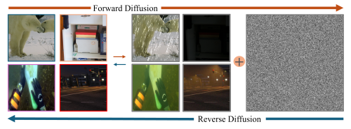
Figure 1: Our ReviveDiff can address a wide range of adverse degradations (such as rain, low light, underwater, and nighttime dehazing) and bring images back to life by enhancing and restoring their quality.

As research has progressed, more complex challenges such as nighttime image defogging [8, 11, 12] and underwater image enhancement [13, 14, 15, 16] have come to the forefront. Although these solutions have shown impressive achievements by employing techniques like Atmospheric Point Spread Function-guided Glow Rendering and posterior distribution processes for underwater color restoration, they remain constrained by their focus on specific degradation scenarios. Their tailored design potentially limits their applicability to other degradations.

Recognizing the limitations of task-specific models, recent efforts such as NAFNet [17], IRSDE [18], and Restormer [19], have aimed to address common degradations with a single neural network architecture, dealing with issues such as blurring, noise, and low resolution. However, these methods often fall short in handling images from particularly challenging environments, such as those captured at night or underwater, which underscores the need for a universal framework capable of concurrently addressing diverse adverse weather conditions.

The root causes of image degradation vary significantly; for example, blurring is typically caused by motion, while noise and low resolution often stem from limitations in imaging equipment. In contrast, quality degradation under adverse conditions is predominantly due to natural phenomena such as fog, water, and low light. This type of degradation generally maintains the structural integrity of objects in the image, leading to less distortion and information loss than other degradation types. These characteristics have inspired us to leverage general image attributes, such as edges, noise levels, and color distortions to guide the distortion process across a wide range of adverse weather conditions, rather than relying on priors specific to an individual task.

To address this need for a more versatile and robust solution, we propose ReviveDiff, a groundbreaking universal diffusion model designed to restore image quality across a wide range of adverse environments. Our approach builds on the strengths of diffusion models, particularly their use of Stochastic Differential Equations (SDE) and Gaussian noise-based features, to create a model capable of handling an expansive feature space with exceptional learning capabilities. Unlike existing models, ReviveDiff is not confined to a single type of degradation but is equipped to tackle a wide range of adverse conditions and restore image qualities.

Specifically, what sets our ReviveDiff apart is its ability to address key factors that determine image quality, such as sharpness, contrast, noise, color accuracy, and distortion, from both a coarse-level overview and a detailed, fine-level perspective. Our model incorporates a novel multi-stage Multi-Attentional Feature Complementation module, which integrates spatial, channel, and point-wise attention mechanisms with dynamic weighting to balance macro and micro information. This design significantly enhances information integration, ensuring that the restored images are not only visually appealing but also retain the structural and color integrity necessary for subsequent tasks. Our comprehensive experiments, conducted across seven benchmark datasets and five types of adverse conditions—Rainy, Underwater, Low-light, Foggy, and Nighttime hazy—demonstrate that ReviveDiff consistently outperforms state-of-the-art methods in both quantitative measures and visual quality. This highlights the model’s broad applicability and its potential to set new standards in image restoration under challenging conditions.

The main contributions of our work are listed as follows:

1. We develop ReviveDiff, a universal framework that can restore image quality across a wide range of adverse weather conditions, representing a significant advancement over the existing task-specific models.

2. We propose a novel Coarse-to-Fine Learning Block (C2FBlock), which not only expands the receptive field through two distinct scale branches but also minimizes information loss. This design enables the network to capture complex and challenging degradations effectively.

3. We design a novel Multi-Attentional Feature Complementation (MAFC) module that integrates spatial, channel, and point-wise attention mechanisms with dynamic weighting. This enhances the model and helps it complement information between macro and micro levels effectively.

4. We introduce a unique prior-guided loss function that ensures optimal pixel restoration by leveraging edge information to refine object shapes and structures while utilizing histogram information to guide accurate color correction under adverse conditions.

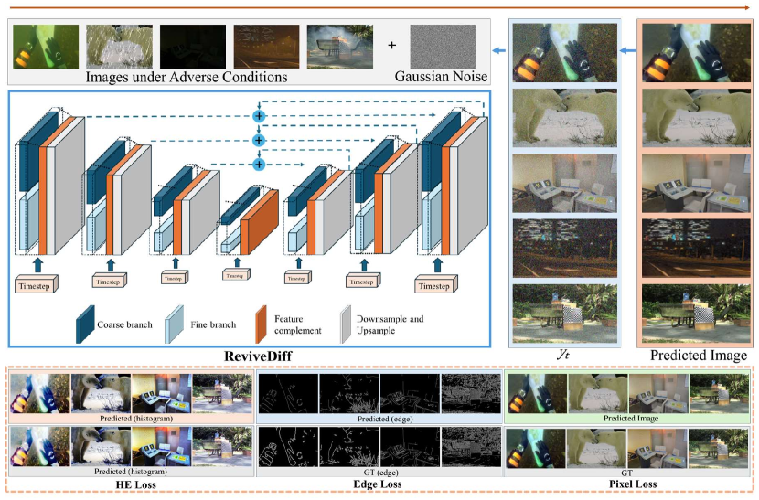
Figure 2: The basic framework of our proposed ReviveDiff, which is a U-shaped based latent diffusion model, with stacked Coarse-to-Fine Learning Blocks (C2FBlock) to tackle diverse real-world image restoration tasks.

II Related Work

In this section, we briefly review recent advancements in image restoration, particularly in challenging environments, and discuss the role of diffusion models in vision tasks.

II-A Image Restoration

Image restoration is a broad field encompassing various tasks aimed at recovering high-quality images from degraded inputs. Classic image restoration tasks include deblurring, denoising, deraining, and super-resolution. Notable contributions in this area include MDARNet by Hao et al. [20], which features a dual-attention architecture specially designed for image deraining, and PREnet by Ren et al., a progressive network designed for rain removal. Additionally, Cui et al. [21] proposed SFNet, which utilizes a multi-branch module with frequency information for image restoration. Uformer [22] employs a U-shaped transformer architecture for this purpose. Zamir et al. [19] introduced Restormer, focusing on high-resolution image restoration, while Tu et al. [23] presented MAXIM, incorporating a multi-axis MLP design.

Additionally, several methods have been designed to address the challenges posed by images captured in adverse conditions. For instance, Zhang et al. [24] developed ReLLIE, a method employing a Markov decision process to enhance low-light images; Li et al. [25] introduced LLFormer, a method integrating Fourier Transform for low-light image restoration. For underwater image restoration, Zhang et al. proposed MLLE [26], which utilizes a novel locally adaptive contrast approach. Peng et al. [13] further enhanced underwater image restoration with a U-shaped transformer that incorporates multi-scale feature fusion. In the domain of nighttime image enhancement, Jin et al. [8] proposed a technique utilizing gradient adaptive convolution, and Yan et al. [12] applied high-low frequency decomposition to recover images affected by nighttime fogging. Although these studies have made significant success, they generally focus on a single task, limiting their applicability across multiple adverse conditions.

II-B Diffusion Models in Vision

The Diffusion models [27, 28] have emerged as powerful tools in the field of image generation and restoration and have achieved significant improvement. These models work by degrading a signal through Gaussian noise and then restoring it through a reverse process. Fei et al. [29] introduced a unified image restoration model that utilizes a diffusion prior, while Lugmayr et al. [3] proposed Repaint, which applies diffusion models, especially to image inpainting. In another significant contribution, Luo et al. proposed IR-SDE [18], which focuses on image restoration through mean-reverting stochastic differential equations.

The application of diffusion models has also extended to enhancing images captured in adverse conditions. For example, Jiang et al. proposed WeatherDiff [10], a wavelet-based diffusion model specially designed for low-light image enhancement. For underwater image enhancement, Du et al. proposed UIEDP [16], which employs a diffusion prior tailored for underwater images, and Tang et al. [30] introduced a transformer-based diffusion model.

The flexibility of diffusion models in accommodating different scenarios in these areas has inspired us to leverage the powerful generalization capabilities of diffusion models to build a universal solution–ReviveDiff– that can effectively address a wide range of adverse degradations. Furthermore, to further enhance its effectiveness in tackling diverse real-world image restoration tasks, we adopted the Mean-Reverting Stochastic Differential Equations (SDEs) based diffusion models [18], which implicitly models the degradation and applies to diverse tasks without changing the architecture.

III Methodology

As illustrated in Fig. 2, our ReviveDiff is a U-shaped based latent diffusion model, with stacked Coarse-to-Fine Blocks (C2FBlocks) and a Multi-Attentional Feature Complementation module to tackle diverse real-world image restoration tasks. Compared with other diffusion models used for image enhancement, our ReviveDiff performs fusion at both low-resolution, macro-level latent space and high-resolution, micro-level latent space from the original input for the decoding process and under the guidance of fine granularity.

Building on the insights from the previous research [18, 31, 17], the C2FBlock introduces a dual-branch structure purposefully designed to capture features at varying levels of granularity. Specifically, as shown in Fig. 3, the Coarse Branch allows the fusion to be performed with a larger receptive field (31 $\times$ 31), enabling it to capture broader contextual information, while the Fine Branch utilizes a focused receptive field of $3\times 3$ to capture finer, more detailed features.

Then, to effectively integrate these coarse and fine features, we developed a Multi-Attentional Feature Complementation module (see Fig. 4), which incorporates three distinct types of attention mechanisms and employs dynamic weighting to adjust the balance between the contributions of Coarse and Fine features. This ensures an optimal balance that enhances the model’s ability to restore image quality across diverse scenarios accurately.

III-A Mean-Reverting Stochastic Differential Processes

In this work, we leverage a probabilistic diffusion approach to enhance visibility in low-light images. Specifically, our approach is based on a score-based generative framework that utilizes Mean-Reverting SDE [18] as the base diffusion framework to model the image-reviving diffusion process. Fig. 2 illustrates this process. The forward SDE gradually transforms the initial data distribution $y_{0}$ into a Gaussian noise representation $y_{T}$ over $T$ steps. The objective of the reverse SDE process is then to reconstruct a high-quality image from this noisy representation $y_{T}$.

Figure 3: The Coarse-to-Fine Learning Block (C2FBlock) at the core of our proposed ReviveDiff network.

Forward SDE: The forward SDE process is defined as the transformation of an input high-quality image into the Gaussian noise. Mathematically, this process is expressed as:

$$dy=\alpha(t)\left(\nu-y\right)dt+\beta(t)dV,$$ (1)

where $\alpha(t)$ regulates the speed of mean reversion, $\beta(t)$ denotes the level of stochastic volatility, and $V$ is the standard Wiener process.

To achieve a solvable form of the forward SDE, we set the condition $\frac{\beta(t)^{2}}{\alpha(t)}=2\kappa^{2}$, with $\kappa^{2}$ symbolizing the stationary variance for any $t\in[0,T]$. Assuming $y(s)$ depicts the noisy image derived from high-quality input at time $s<t$, the solution to Eq. 1 is given by [18]:

$$y(t)=\nu+(y(s)-\nu)e^{-\hat{\alpha}(s:t)}+\int_{s}^{t}\beta(u)e^{-\hat{\alpha}(u:t)}dV(u),$$ (2)

where $\hat{\alpha}(s:t)=\int_{s}^{t}\alpha(u)du$. The distribution of $y_{t}$ is determined as follows:

$$y_{t}\sim p_{t}(y)=\mathcal{N}(y_{t}|\mu_{t}(y),\sigma_{t}^{2}),$$ (3)

where

$$\mu_{t}(y)=\mu+(y(s)-\mu)\mathrm{e}^{-\hat{\alpha}(s:t)},$$ (4)

and

$$\sigma_{t}^{2}=\kappa^{2}\left(1-\mathrm{e}^{-2\hat{\alpha}(s:t)}\right).$$ (5)

Reverse SDE: The goal of the Reverse SDE process is to reconstruct the high-quality image from its degraded representation $y(T)$. As established in earlier research, the reverse SDE is formulated as:

$$dy=\left[\alpha(t)(\nu-y)-\beta(t)^{2}\nabla_{y}\log p_{t}(y)\right]dt+\beta(t)d\tilde{V},$$ (6)

where $\tilde{V}$ signifies another instance of the Wiener process.

The training mechanism utilizes high-quality images to enable the calculation of the gradient score:

$$\nabla_{y}\log p_{t}(y)=-\frac{y(t)-\mu_{t}(y)}{\sigma_{t}^{2}},$$ (7)

facilitating the sampling of $y(t)$ as $y(t)=\mu_{t}(y)+\sigma_{t}\zeta_{t}$, with $\zeta_{t}\sim\mathcal{N}(0,I)$ indicating Gaussian noise.

Thus, the score function is derived as:

$$\nabla_{y}\log p_{t}(y)=-\frac{\zeta_{t}}{\sigma_{t}}.$$ (8)

Figure 4: Coarse and fine features are integrated adaptively and complementarily with our Multi-Attentional Feature Complementation (MAFC) module in our proposed ReviveDiff.

III-B Coarse-to-Fine Learning

Unlike the existing diffusion models used for image enhancement, our ReviveDiff performs feature fusion in the latent space at both macro and micro levels and fuses them under the guidance of fine granularity. This is achieved through a series of stacked C2FBlocks that lie at the core of the U-Net architecture.

As illustrated in Fig. 3, our C2FBlock is specially designed to capture features at two distinct levels of granularity: The Fine Branch is responsible for capturing the image’s detailed, localized features, with a small receptive field, whereas the Coarse Branch operates on a significantly larger receptive field, focusing on the image’s global contextual information in low-resolution space. This dual-branch approach ensures that both macro-level contextual information and detailed, pixel-level details are effectively captured and integrated.

In addition, to improve computational efficiency, we adopt the Simple Gate (SC) activation [17] to replace more complex nonlinear activation functions. The Simple Gate achieves the effect of nonlinear activation using a single multiplication operation, which is especially advantageous in preserving critical information in regions of low pixel values.

Specifically, let $\mathcal{F}_{in}$ represent the input feature. The features extracted by the Fine Branch can be represented as:

$$\mathcal{F^{\prime}}_{fine}=DWConv(LayerNorm(\alpha_{1}\odot\mathcal{F}_{in}+\beta{1})).$$ (9)

The Fine Branch uses a $3\times 3$ receptive field to capture detailed local features, producing $\mathcal{F^{\prime}}_{fine}$. Then, the final output of the Fine Branch $\mathcal{F}_{fine}$ is computed using SimpleGate as $SG$ and a Simplified Channel Attention as $SCA$, as:

$$\mathcal{F}_{fine}=SCA(SG(\mathcal{F^{\prime}}_{fine})).$$ (10)

In contrast to the Fine Branch, the Coarse Branch focuses on global information and operates on a significantly large receptive field of $31\times 31$, as depicted in Fig. 4. However, existing approaches such as the non-local mechanism, vision transformer blocks, and convolutional layers with large kernel sizes, tend to be computationally expensive, consuming significant resources and slowing down processing speeds. To address this issue, we utilize grouped-dilated convolutions to efficiently expand the receptive field size without substantially increasing the computation load.

To mitigate the information loss due to the gridding effect commonly associated with dilated convolutions, we employ a stacking strategy rather than a single convolutional layer. Specifically, we apply increasing dilation rates of 2-4-8 to achieve a large receptive field while minimizing the loss of fine-grained details. Finally, grouped convolutions are used to prevent a substantial increase in parameters, ensuring that the model remains computationally efficient.

Thus, denoting grouped-dilated convolution with a dilation rate of $i$ as $f_{r=i}$, the Coarse Feature, $\mathcal{F}_{coarse,size}$, where $size$ represents its kernel size, can be obtained as:

$$\left.\left\{\begin{array}[]{ll}\mathcal{F}_{coarse,7\times 7}=f_{r=2}(\mathcal{F}_{fine})\\ \mathcal{F}_{coarse,15\times 15}=f_{r=4}(\mathcal{F}_{coarse,7\times 7})\\ \mathcal{F}_{coarse,31\times 31}=f_{r=8}(\mathcal{F}_{coarse,15\times 15})\end{array}\right.\right..$$ (11)

This coarse-to-fine learning process enables our model to capture both broad contextual information and focused local details, ensuring a balanced and thorough restoration of images across different types of degradations. As experimental results show, by fusing coarse and fine features in latent space, our ReviveDiff achieves superior performance in a range of challenging image enhancement tasks.

(a)

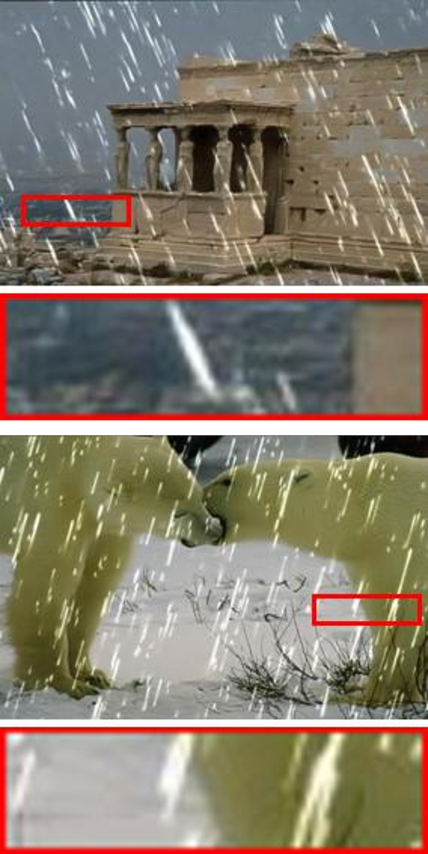
(b)

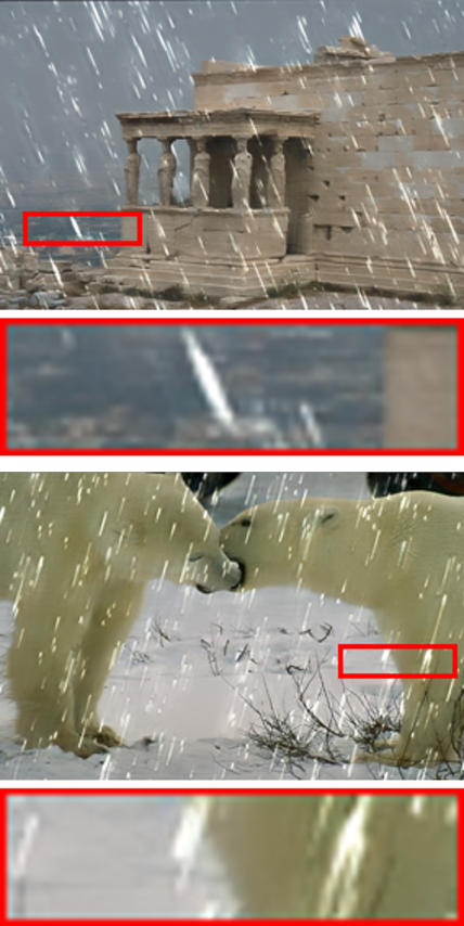
(c)

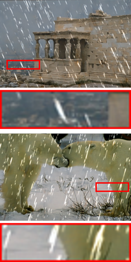
(d)

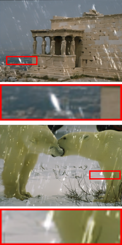
(e)

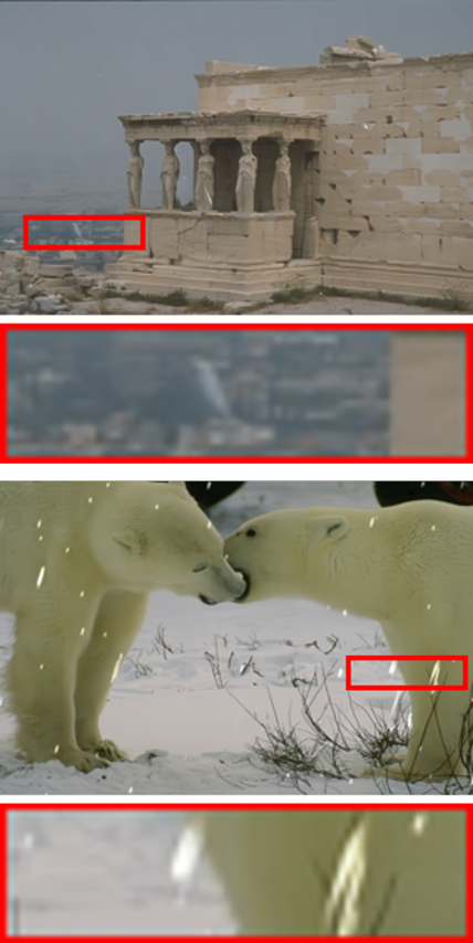
(f)

(g)

(h)

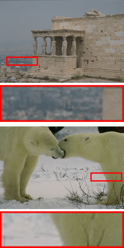
(i)

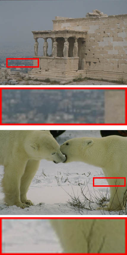
(j)

Figure 5: Visual comparison of the deraining results obtained with our ReviveDiff and SOTA approaches on Rain100L [36]. The small images enclosed in red below each result provide an enlarged view of the areas highlighted by red rectangles.

TABLE I: Comparison of image deraining results with SOTAs on the Rain100L Deraining dataset [36].

Methods	DerainNet [6]	SEMI [33]	UMRL [34]	DIDMDN [32]	Jorder [37]	MSPFN [38]	SPAIR [39]	MPRNET [35]	MAXIM [23]	MDARNet [20]	SFNet [21]	AWRaCLe [40]	FMRNET [41]	ReviveDiff
PSNR $\uparrow$	27.03	25.03	29.18	25.23	36.61	32.4	37.3	36.4	38.06	35.68	38.21	35.71	37.81	39.09
SSIM $\uparrow$	0.884	0.842	0.923	0.741	0.974	0.933	0.978	0.965	0.977	0.961	0.974	0.966	0.974	0.979
LPIPS $\downarrow$	/	/	/	/	0.028	/	/	0.077	0.048	/	/	/	/	0.012

III-C Multi-Attentional Feature Complementation

Given the Fine Features $\mathcal{F}_{fine}$ and the Coarse Features $\mathcal{F}_{coarse}$ obtained from Coarse-to-Fine Learning, the significant granularity gap between them poses a challenge for effective fusion and refinement.

To address this issue, we propose a Multi-Attentional Feature Complementation (MAFC) module, which utilizes attention-based mechanisms [42] to dynamically compute feature weights both spatially [43] and across channels [44]. This allows for realignment and complementary fusion of the Coarse and Fine features, ensuring that the resulting feature map maintains critical information from both levels of granularity adaptively and complementarily.

For spatial dimension alignment, we utilize a spatial attention mechanism to learn the spatial weight map $W_{\text{s}}\in\mathbb{R}^{H\times W}$. This map highlights the importance of different regions within an image. Meanwhile, the channel weight is computed as $W_{\text{c}}\in\mathbb{R}^{C\times 1\times 1}$, indicating the importance of each channel for a given task.

Denote $\mathcal{F}_{C2F}=\mathcal{F}_{coarse}+\mathcal{F}_{fine}$ as the feature map integrating both Coarse and Fine Features, the spatial weight $W_{\text{s}}$ and the channel weight $W_{\text{c}}$ can be calculated as:

$$\left.\left\{\begin{array}[]{ll}W_{s}&={Cov}_{7\times 7}([GAP_{s}(\mathcal{F}_{C2F}),GMP_{s}(\mathcal{F}_{C2F})]),\\ W_{c}&={Conv}_{1\times 1}(ReLU({Conv}_{1\times 1}(GAP_{c}(\mathcal{F}_{C2F}))).\end{array}\right.\right.$$ (12)

Here, $GAP$ refers to Global Average Pooling, $GMP$ denotes Global Max Pooling, and $s$ and $c$ indicate that the GAP/GMP operation is conducted along the spatial or channel dimensions, respectively.

Thus, the combination weight $W_{C2F}$ recalibrating $\mathcal{F}_{coarse}$ and $\mathcal{F}_{fine}$ can be defined as:

$$W_{C2F}=\sigma(W_{s}+W_{c}),$$ (13)

where $\sigma$ denotes the Sigmoid function.

Furthermore, to further refine the fine features $\mathcal{F}_{fine}$, we employ a Pixel Attention [45] scheme to establish attention coefficients at the pixel level, aiming to obtain a more sophisticated feature map $\mathcal{F^{\prime}}_{fine}$:

$$\mathcal{F^{\prime}}_{fine}=\sigma(Conv_{1\times 1}(\mathcal{F}_{fine})\cdot\mathcal{F}_{fine}).$$ (14)

Finally, the feature map $\mathcal{F}_{fused}$ can be generated by weighted recalibration as:

$$\mathcal{F}_{fused}=Conv_{1\times 1}(\mathcal{F^{\prime}}_{fine}\cdot W_{C2F}+\mathcal{F}_{coarse}\cdot(1-W_{C2F})).$$ (15)

Then, the fused feature $\mathcal{F}_{fused}$ is processed with Layer Normalization (LN) and subsequently modified by the scale and shift factors $\alpha_{2}$ and $\beta_{2}$ as:

$$\mathcal{F^{\prime}}_{out}=LM(\alpha_{2}\odot\mathcal{F}_{fused}+\beta_{2}).$$ (16)

Finally, the output feature of the C2FBlock, denoted as $\mathcal{F}_{out}$, is obtained as:

$$\mathcal{F}_{out}=Conv_{1\times 1}(SG(Conv_{1\times 1}(\mathcal{F^{\prime}}_{out}))).$$ (17)

This multi-Attentional feature complementation allows for highly effective integration of Coarse and Fine features, ensuring that both global context and fine details are preserved and enhanced. This results in a feature map that is not only contextually aware but also rich in local details, providing the foundation for superior image restoration performance.

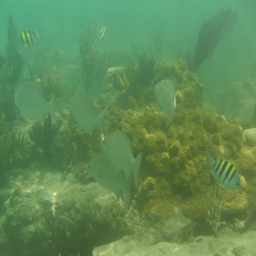
(a)

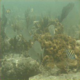
(b)

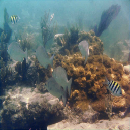
(c)

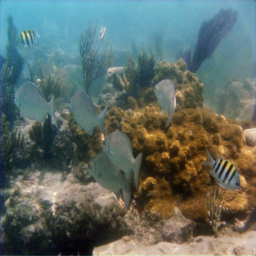
(d)

(e)

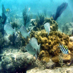
(f)

(a)

(b)

(c)

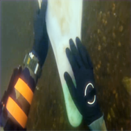
(d)

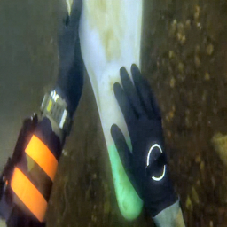
(e)

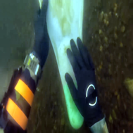
(f)

(a) With-Reference Results

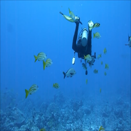
(a)

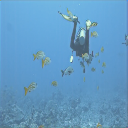
(b)

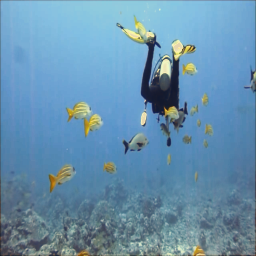
(c)

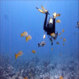
(d)

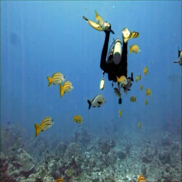
(e)

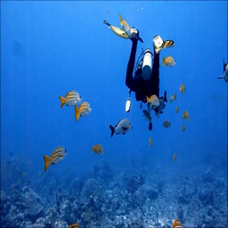
(f)

(a)

(b)

(c)

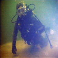
(d)

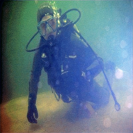
(e)

(f)

(b) Non-Reference Results

Figure 6: Visual comparison of underwater image enhancement results with SOTAs on T90 [48], U45 [49], and C60 [48].

TABLE II: Quantitative comparison results of underwater image enhancement with SOTAs on the T90 [48], U45 [49], and C60 [48] underwater datasets.

Dataset	Methods	GDCP [50]	UGAN [51]	FUnIEGAN [52]	UWCNN [46]	Ucolor [53]	MLLE [26]	UShape [13]	FA+Net [14]	NU2Net [15]	ReviveDiff
T90	PSNR $\uparrow$	13.89	17.42	16.97	19.02	20.86	19.48	20.24	20.98	22.93	25.01
	SSIM $\uparrow$	0.75	0.76	0.73	0.82	0.88	0.84	0.81	0.88	0.90	0.92
	NIQE $\downarrow$	4.93	5.81	4.92	4.72	4.75	4.87	4.67	4.83	4.81	4.45
U45	UCIQE $\uparrow$	0.59	0.57	0.56	0.48	0.58	0.59	0.57	0.58	0.57	0.62
	NIQE $\downarrow$	4.14	5.79	4.45	4.09	4.71	4.83	4.20	4.02	5.7	3.93
C60	UCIQE $\uparrow$	0.57	0.55	0.55	0.51	0.55	0.57	0.56	0.57	0.58	0.59
	NIQE $\downarrow$	6.27	6.90	6.06	5.94	6.14	5.85	5.60	5.70	5.64	5.57

III-D Prior-Guided Loss Functions

In many related research fields, pixel-based loss functions such as L1, MSE, PSNR [54], and SSIM [55] Losses are widely used. These loss functions aim to minimize pixel-wise differences between the generated image $I_{\text{gen}}$ and the ground truth image $I_{\text{gt}}$. The Pixel-based Loss, $L_{\text{pixel}}$, is defined as:

$$L_{\text{pixel}}(I_{\text{gen}},I_{\text{gt}})=\frac{1}{N}\sum_{i=1}^{N}|I_{\text{gen},i}-I_{\text{gt},i}|,$$ (18)

where $N$ denotes the total number of pixels in the image.

However, for low-quality images captured from adverse natural conditions, visibility is predominantly affected by the medium of light propagation, such as fog or underwater environments, rather than by distortion or blur. As a result, objects within these images tend to retain their regular edges, shapes, and structures, even though overall visibility may be compromised. Leveraging this observation, incorporating edge and color information into the loss function can further enhance the training process by ensuring that key structural and color features are preserved during restoration and thus be advantageous.

III-D1 Edge Loss

In our study, to preserve structural information, we introduce an Edge Loss that focuses on maintaining the integrity of edges in the enhanced image. We utilize the Canny edge detector to extract the edge information from both the enhanced image $I_{\text{gen}}$ and the corresponding reference image $I_{\text{gt}}$. The Edge Loss, $L_{\text{edge}}$, is defined as:

$$L_{\text{edge}}(I_{\text{gen}},I_{\text{gt}})=\left\|\mathcal{E}(I_{gen};\sigma,T_{\text{low}},T_{\text{high}})-\mathcal{E}(I_{gt};\sigma,T_{\text{low}},T_{\text{high}})\right\|_{1}.$$ (19)

Here, $\mathcal{E}(\cdot;\sigma,T_{\text{low}},T_{\text{high}})$ denotes the edge map obtained by applying the Canny edge detector with a Gaussian smoothing parameter $\sigma$ and hysteresis thresholding parameters $T_{\text{low}}$ and $T_{\text{high}}$. The Canny edge detection process, $\mathcal{E}$, includes gradient magnitude computation using a Gaussian filter with standard deviation $\sigma$, non-maximum suppression, and edge tracking by hysteresis using thresholds $T_{\text{low}}$ and $T_{\text{high}}$. The $\text{L}_{1}$ norm $\left\|\cdot\right\|_{1}$ calculates the sum of absolute differences between the edge maps of the enhanced and reference images, ensuring the preservation of edge information during image enhancement.

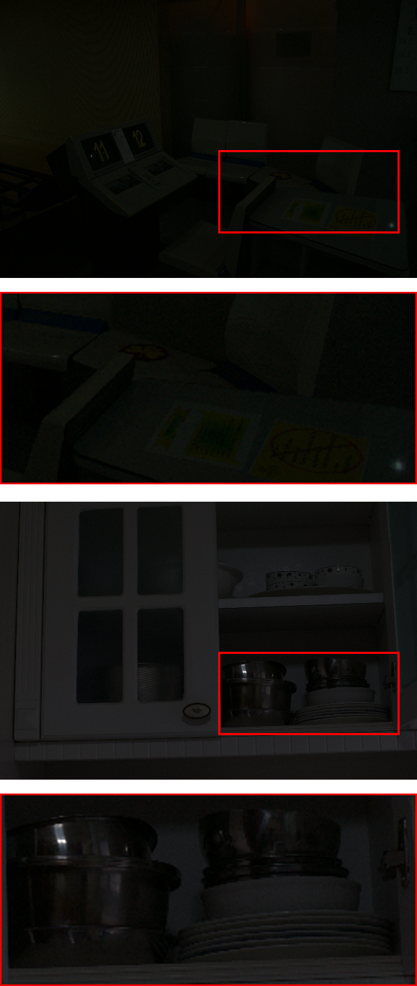
(a)

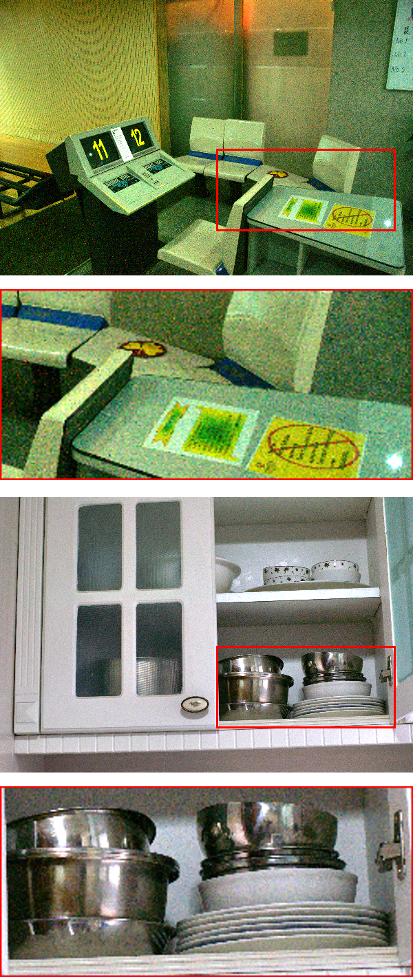
(b)

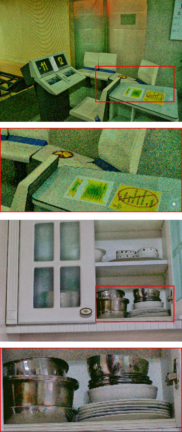
(c)

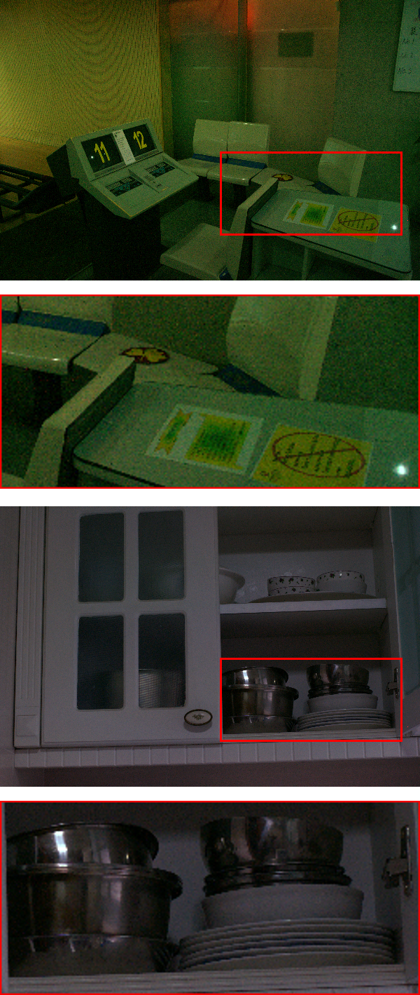
(d)

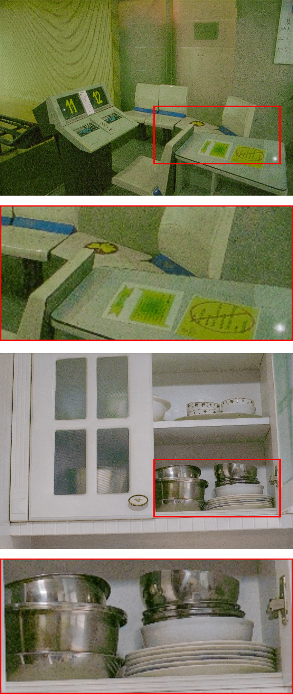
(e)

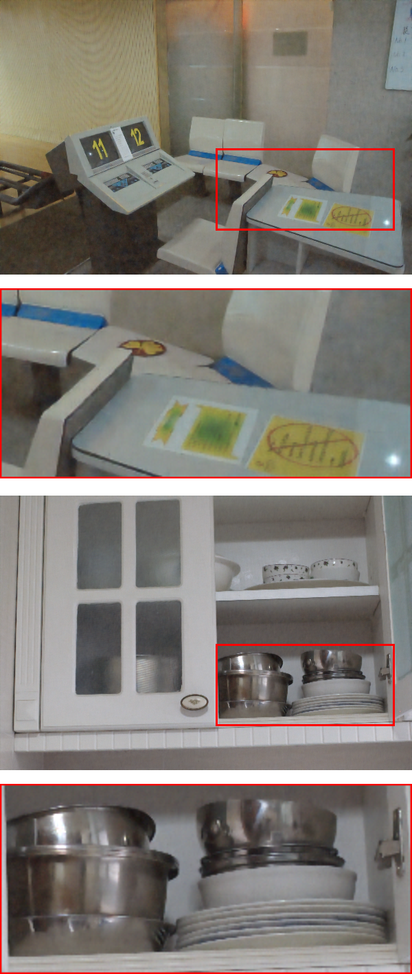
(f)

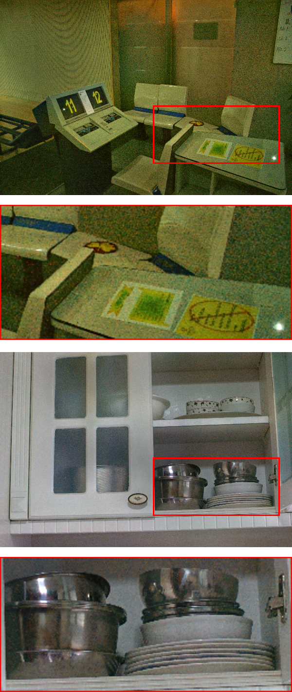
(g)

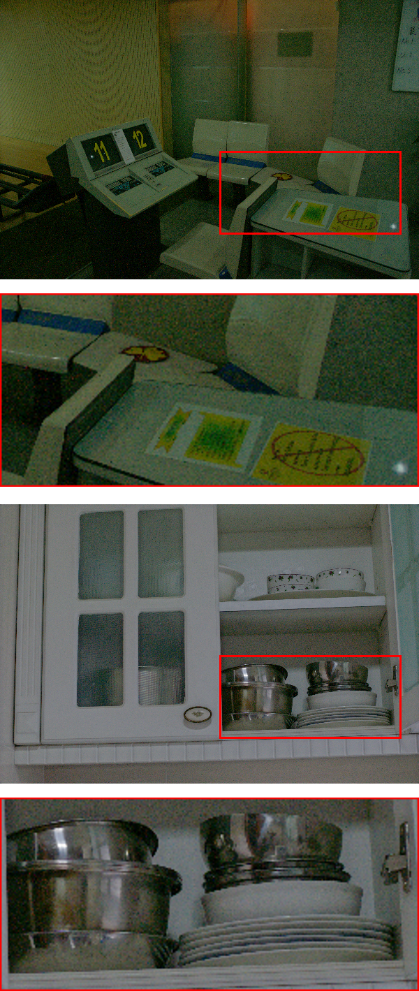
(h)

(i)

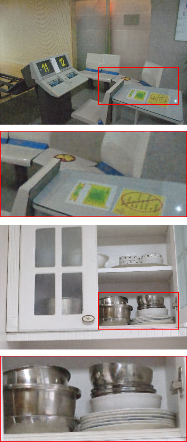
(j)

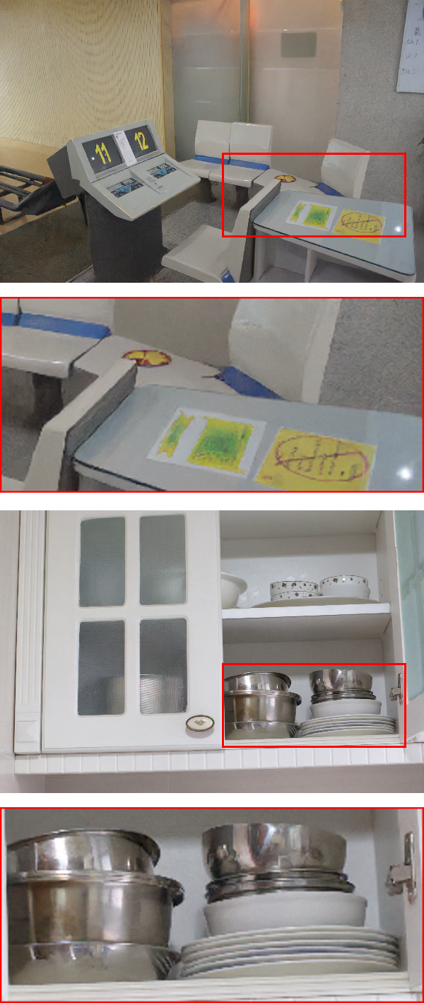
(k)

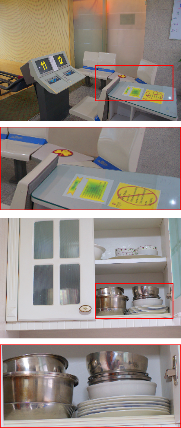
(l)

Figure 7: Visual comparison of low-light image enhancement results with SOTAs on the LOL dataset [63]. The small images enclosed in red below each result provide an enlarged view of the areas highlighted by red rectangles.

III-D2 Histogram Loss

To ensure color consistency, we introduce a Histogram Loss to measure the discrepancy in color distribution between the enhanced image $I_{\text{gen}}$ and the corresponding reference image $I_{\text{gt}}$ in $R$, $G$, and $B$ channels, respectively. The Histogram Loss, $L_{\text{hist}}$, can be defined as:

$$L_{\text{hist}}(I_{\text{gen}},I_{\text{gt}})=\sum_{c=1}^{C}\left\|\frac{H(I_{\text{gen},c},k)}{\sum_{k=1}^{K}H(I_{\text{gen},c},k)}-\frac{H(I_{\text{gt},c},k)}{\sum_{k=1}^{K}H(I_{\text{gt},c},k)}\right\|_{1},$$ (20)

where the $H(I_{\text{gen},c},k)$ and $H(I_{\text{gt},c},k)$ are the histogram counts for the $k$-th bin in the $c$-th channel of the enhanced and reference images, respectively. $K$ denotes the total number of bins. The L1 norm $\left\|\cdot\right\|_{1}$ is used to calculate the sum of absolute differences between the normalized histograms of the enhanced and reference images across all bins and channels. This term ensures that the color distribution in the enhanced image closely matches that of the reference image, which is particularly important in challenging environments where color distortion is common.

TABLE III: Quantitative comparison of low-light image enhancement results on the LOL dataset [63] in terms of PSNR (dB), SSIM, and LPIPS.

Methods	RetinexNet [5]	KIND [64]	DSLR [65]	DRBN [66]	Zero-DCE [61]	MIRNet [67]	EnlightenGAN [60]	ReLLIE [24]	RUAS [62]	KIND++ [68]	DDIM [27]
PSNR $\uparrow$	16.774	20.84	14.816	16.774	14.816	24.138	17.606	11.437	16.405	21.300	16.521
SSIM $\uparrow$	0.462	0.790	0.572	0.462	0.572	0.830	0.653	0.482	0.503	0.820	0.776
LPIPS $\downarrow$	0.417	0.170	0.375	0.417	0.375	0.250	0.372	0.375	0.364	0.160	0.376
Methods	CDEF [69]	SCI [70]	URetinex-Net [5]	Uformer [22]	Restormer [19]	Palette [71]	UHDFour [9]	WeatherDiff [10]	LLformer [25]	LightenDiffusion [72]	ReviveDiff
PSNR $\uparrow$	16.335	14.784	19.842	19.001	20.614	11.771	23.093	17.913	23.650	20.453	24.272
SSIM $\uparrow$	0.585	0.525	0.824	0.741	0.797	0.561	0.821	0.811	0.816	0.803	0.832
LPIPS $\downarrow$	0.407	0.366	0.237	0.354	0.288	0.498	0.259	0.272	0.171	0.192	0.0875

III-D3 Combined Loss

The overall loss function used to guide the training of our model combines the pixel-wise, edge, and histogram losses to ensure that the restored image maintains not only pixel-level accuracy but also structural integrity and accurate color representation.

The combined loss, $L$, is formulated as:

$$L=\lambda_{\text{1}}L_{\text{pixel}}(I_{\text{gen}},I_{\text{gt}})+\lambda_{\text{2}}L_{\text{edge}}(I_{\text{gen}},I_{\text{gt}})+\lambda_{\text{3}}L_{\text{hist}}(I_{\text{gen}},I_{\text{gt}}).$$ (21)

Here, $\lambda_{\text{1}}$, $\lambda_{\text{2}}$, and $\lambda_{\text{3}}$ are the learned weighting coefficients that dynamically balance the contributions of the Pixel-wise loss, Edge loss, and Histogram loss, respectively.

These weights allow the model to focus on different aspects of image quality—pixel-level accuracy, edge preservation, and color consistency—based on the specific degradation present in the input image.

IV Experiments

To demonstrate the superior performance of our proposed ReviveDiff approach in enhancing image visibility under adverse conditions, we designed comprehensive experiments that benchmark our approach with SOTA approaches on five challenging tasks: image deraining, low-light image enhancement, nighttime dehazing, defogging, and underwater image enhancement. Next, we first introduce the datasets and experiment details. Then, we present experimental comparisons with SOTA approaches and ablation studies on the key modules in our approach.

IV-A Datasets

Image Deraining: For the image deraining task, we evaluated our ReviveDiff model using the Rain100L [36] dataset, which includes both clean and synthetic rainy images, with 200 pairs for training and 100 for testing.
Underwater Image Enhancement: For the underwater image enhancement task, we used three datasets: the UIEB dataset [48], the C60 [48] dataset, and the U45 dataset [49]. The UIEB dataset consists of 890 pairs of low-quality and high-quality images, while the C60 and U45 datasets comprise 60 and 45 challenging images, respectively, without reference images. Consistent with previous works, we split the UIEB dataset into 800 pairs for training and 90 images for testing (referred to as “T90”). We tested our ReviveDiff on all these three datasets.
Low-light Image Enhancement: For the low-light image enhancement task, we evaluated our ReviveDiff on the LOw-Light (LOL) [63] dataset, which comprises 500 image pairs of synthetic low-light and normal-light images. The LOL dataset provides 485 pairs for training and 15 pairs for testing.
Nighttime Dehazing: For the nighttime dehazing task, we used the GTA5 [73] dataset, a synthetic dataset created with the GTA5 game engine. The GTA5 dataset includes 864 image pairs, with 787 of them designated for training and the remaining 77 pairs for testing.
Image Defogging: For the image defogging task, we utilized the SMOKE [74] dataset, which consists of 132 paired real-world images captured in natural scenes with fog generated by a fog machine. 120 pairs of these images are used for training and the remaining 12 pairs for testing.

(a)

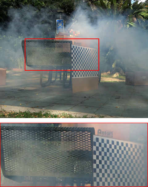
(b)

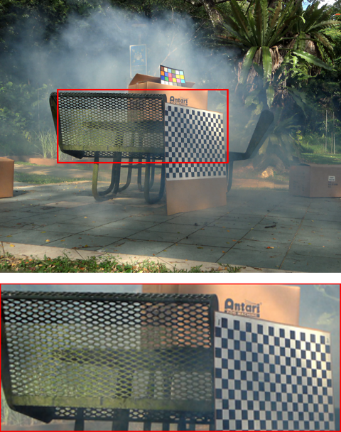
(c)

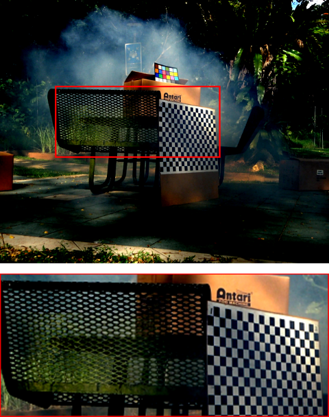
(d)

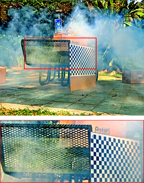
(e)

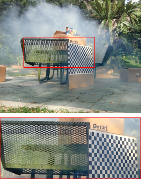
(f)

(g)

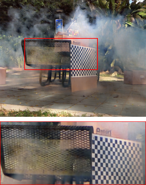
(h)

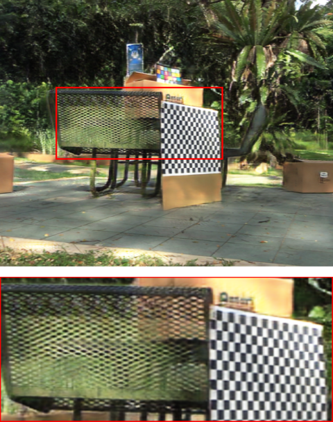
(i)

(j)

Figure 8: Visual comparison of smoke image enhancement results with SOTAs on the SMOKE dataset [74].

IV-B Implementation Details

During model training, we utilized a batch size of 4 and initialized the learning rate to $1\times 10^{-4}$. We used the Adam optimizer [82], with parameters $\beta_{1}$ and $\beta_{2}$ to 0.9 and 0.999, for training optimization. The learning rate was adjusted using the MultiStepLR strategy for decay. The total number of training iterations varied based on the specific degradation being addressed. We employed a noise level of $\sigma=90$ and set the diffusion step to 300 for all tasks. All experiments were conducted on a single NVIDIA RTX 4090 GPU using the PyTorch platform.

IV-C Comparisons with the State of the Arts

IV-C1 Image Deraining

Images captured in rainy conditions often suffer from the detrimental effects of rain streaks. To evaluate our method’s deraining capability, we utilized three widely recognized metrics: PSNR [54], SSIM [55], and LPIPS [83]. We compared our method with several SOTAs from 2016 to 2023.

As demonstrated in Table I, our ReviveDiff model achieves the highest scores across all these metrics. When compared to the second-best method, SFNet [21], our PSNR surpassed it by 0.88, making ReviveDiff the only method to achieve a PSNR over 39. This indicates the superior quantitative performance of our ReviveDiff in deraining. Visually, as depicted in Fig. 5, our results show a significant reduction in rain presence and are most closely aligned with the reference image in terms of quality.

IV-C2 Underwater Image Enhancement

Underwater images often suffer from degradation due to the scattering and absorption effects of water, coupled with low illumination, resulting in poor visual quality. In our study, we evaluated ReviveDiff using both paired (T90) and non-reference datasets (U45 and C60). For the T90 dataset, we employed widely recognized metrics: PSNR and SSIM, to assess image quality. Additionally, we utilized two metrics that do not require reference images for computation: UCIQE [84] (to evaluate brightness) and NIQE [85] (to assess distortion and noise). These metrics were also applied to the U45 and C60 datasets. We compared our ReviveDiff model with SOTAs [47], among which GDCP [50] represents traditional theory-based approaches, while the others are deep learning-based.

For a quantitative comparison, as shown in Table II, our ReviveDiff outperforms all other methods across all three datasets. Specifically, ReviveDiff achieves exceptional performance in PSNR and SSIM metrics. Compared to the second-best method, NU2Net [15], our PSNR is higher by 4.03 (an improvement of 19%), and ReviveDiff is the only method to achieve an SSIM greater than 0.9. Furthermore, on the U45 dataset, the proposed ReviveDiff is the only method to achieve a NIQE score lower than 4, indicating its superior restoration performance of brightness.

For visual quality comparison, as illustrated in Fig. 6, our ReviveDiff generates results that are most similar to the reference images in the T90 dataset. Additionally, for the non-reference datasets U45 and C60, our results also demonstrate better visual quality.

IV-C3 Low-light Image Enhancement

Enhancing the image quality of low-light images is a significant challenge in current research. To assess the performance of our ReviveDiff model, we employed metrics such as PSNR, SSIM, and LPIPS, and compared our results with state-of-the-art (SOTA) methods from 2018 to 2023.

As shown in Table III, our ReviveDiff model outperforms competing approaches across these metrics. Notably, our method is the only one to achieve an LPIPS score lower than 0.1, signifying unparalleled results in terms of human visual perception. Furthermore, as depicted in Fig. 7, our results demonstrate superior visual quality, exhibiting minimal color distortion and optimal brightness, closely matching the ground truth images.

IV-C4 Nighttime Image Dehazing

Nighttime image Dehazing presents a highly complex task, requiring methods that preserve the low-light environment while simultaneously removing haze. As demonstrated in Table V, our ReviveDiff model surpasses SOTAs in both PSNR and LPIPS metrics, experiencing a marginal loss in SSIM by only 0.009 (1%) compared to the method by Jin et al. [8]. However, our ReviveDiff model outperforms that of Jin et al. in PSNR by 2.53 (8%), and a lower LPIPS score indicates better alignment with human perception. This is further supported by visual quality comparisons in Fig. 9, where it is evident that the method by Jin et al. [8] fails to restore light as effectively as ours, resulting in darker images with lower contrast.

TABLE IV: Comparison of image defogging with SOTAs on the SMOKE dataset [74] in terms of PSNR (dB) and SSIM.

Method	PSNR $\uparrow$	SSIM$\uparrow$
DCP [86]	11.26	0.26
GDN [87]	15.19	0.53
MSBDN [80]	13.19	0.34
DeHamer [75]	13.31	0.28
SMOKE [74]	18.83	0.62
Ours	19.97	0.64

IV-C5 Image Defogging

Image defogging is a challenging task that requires methods capable of effectively removing dense fog while preserving the underlying image details and maintaining natural visibility.

Fig. 8 presents a visual comparison of defogging results produced by different methods. The input image, heavily affected by smoke, is processed by a variety of SOTA techniques. As illustrated, our method achieves the most visually appealing result, effectively removing the smoke and recovering scene details with high fidelity. In contrast, other methods either leave residual smoke or introduce noticeable artifacts, leading to less satisfactory results.

Table IV shows a quantitative comparison of defogging performance. As shown in this table, our method achieves the highest PSNR of 19.97 dB and SSIM of 0.64, outperforming other SOTA methods such as SMOKE [74] (PSNR 18.83 dB, SSIM 0.62). This significant improvement highlights the superior capability of our method in restoring clear images while preserving structural information. Both the visual and quantitative comparisons demonstrate that our approach surpasses existing techniques, achieving state-of-the-art performance in the image-defogging task.

IV-D Ablation Studies

We conducted further ablation studies to validate the effectiveness of the proposed key components: Coarse-to-Fine Learning, Multi-Attentional Feature Complementation and Guided Losses of Edge and Histogram Priors. We select the challenging task of nighttime image defogging to conduct ablation studies on our proposed method. Table V presents a detailed comparison.

IV-D1 Effectiveness of Coarse-to-Fine Learning

As shown in Table V, our model, even without Coarse-to-Fine Learning (referred to as $w/o\ C2F$), outperforms the second comparison method by Jin et al. [8]. However, it falls short of ReviveDiff in terms of PSNR, SSIM, and LPIPS metrics. This underscores the importance of Coarse-to-Fine Learning.

IV-D2 Effectiveness of Multi-attentional Feature Complementation

In Table V, the variant labeled $w/o\ MAFC$ employs a simple addition operation instead of multi-attentional feature complementation to combine the features. As shown in this table, the noticeable decline in performance without the MAFC module indicates the model’s inability to effectively balance the weights of Coarse and Fine features, significantly reducing its effectiveness.

IV-D3 Effectiveness of the Prior-Guided Losses

As shown in Fig. 9 and Table V, experiments denoted as $w/o\ Edge\ Prior$ and $w/o\ His\ Prior$ reveal that lacking these two types of guidance, the model struggles to accurately restore the object’s edges and colors. The outcome under the $Only\ L_{1}\ Loss$ condition further confirms that relying solely on a single $L_{1}$ loss function, without prior-guided support, is insufficient for our ReviveDiff to learn and correct the degradation in low-quality images.

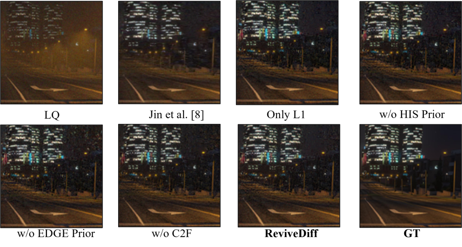
Figure 9: Visual comparison of the nighttime dehazing results with the benchmark approach by Jin et al. [8] and ablation studies on the Prior-Guided Losses on the GTA5 nighttime hazing dataset [73].

TABLE V: Comparison with SOTAs and ablation studies on the GTA5 Nighttime hazing dataset [73].

Method	PSNR $\uparrow$	SSIM $\uparrow$	LPIPS $\downarrow$
Li et al. [11]	21.02	0.639	-
Zhang et al. [88]	20.92	0.646	-
Ancuti et al. [89]	20.59	0.623	-
Yan et al. [12]	27.00	0.850	-
CycleGAN [90]	21.75	0.696	-
Jin et al. [8]	30.38	0.904	0.099
IR-SDE [18]	31.34	0.856	0.098
Only $L_{1}$ Loss	30.82	0.840	0.103
$w/o$ Edge Prior	30.56	0.838	0.107
$w/o$ His Prior	30.49	0.837	0.106
$w/o$ MAFC	23.77	0.722	0.206
$w/o$ C2F	32.52	0.840	0.098
ReviveDiff	32.91	0.895	0.094

V Conclusion

In this paper, we developed a novel diffusion model “ReviveDiff” specifically designed for enhancing images degraded by diverse adverse environmental conditions such as fog, rain, underwater scenarios, and nighttime settings. ReviveDiff features a unique Coarse-to-Fine Learning framework and a Multi-Attention Feature Complementation module, enabling the effective learning and fusion of multi-scale features. Additionally, it incorporates edge and histogram priors for enhanced structure and color restoration. Upon evaluation across seven datasets that cover a range of adverse degradations, ReviveDiff demonstrably outperforms existing SOTAs, offering a robust solution for universal adverse condition image enhancement challenges. To our knowledge, our ReviveDiff represents a breakthrough contribution, utilizing a diffusion-based universal approach to address adverse conditions. This work not only underscores the versatility and efficacy of diffusion models in restoring images affected by adverse conditions but also establishes a new benchmark for future research in the field.

References

- [1] Q. Zhu, M. Zhou, N. Zheng, C. Li, J. Huang, and F. Zhao, “Exploring temporal frequency spectrum in deep video deblurring,” in Proceedings of the IEEE/CVF International Conference on Computer Vision, 2023, pp. 12 428–12 437.
- [2] J. Liu, Q. Wang, H. Fan, Y. Wang, Y. Tang, and L. Qu, “Residual denoising diffusion models,” in Proceedings of the IEEE/CVF Conference on Computer Vision and Pattern Recognition, 2024, pp. 2773–2783.
- [3] A. Lugmayr, M. Danelljan, A. Romero, F. Yu, R. Timofte, and L. Van Gool, “Repaint: Inpainting using denoising diffusion probabilistic models,” in Proceedings of the IEEE/CVF Conference on Computer Vision and Pattern Recognition, 2022, pp. 11 461–11 471.
- [4] H. Zhu, P. Xi, V. Chandrasekhar, L. Li, and J. H. Lim, “Dehazegan: When image dehazing meets differential programming,” in Proceedings of the International Joint Conference on Artificial Intelligence, 2018, pp. 1234–1240.
- [5] C. Wei, W. Wang, W. Yang, and J. Liu, “Deep retinex decomposition for low-light enhancement,” in Proceedings of the British Machine Vision Conference, 2019.
- [6] X. Fu, J. Huang, X. Ding, Y. Liao, and J. W. Paisley, “Clearing the skies: A deep network architecture for single-image rain removal,” IEEE Transactions on Image Processing, vol. 26, pp. 2944–2956, 2016.
- [7] E. H. Land, “The retinex theory of color vision,” Scientific american, vol. 237, no. 6, pp. 108–129, 1977.
- [8] Y. Jin, B. Lin, W. Yan, Y. Yuan, W. Ye, and R. T. Tan, “Enhancing visibility in nighttime haze images using guided apsf and gradient adaptive convolution,” in Proceedings of the ACM International Conference on Multimedia, 2023, pp. 2446–2457.
- [9] C. Li, C.-L. Guo, M. Zhou, Z. Liang, S. Zhou, R. Feng, and C. C. Loy, “Embedding fourier for ultra-high-definition low-light image enhancement,” arXiv preprint arXiv:2302.11831, 2023.
- [10] H. Jiang, A. Luo, H. Fan, S. Han, and S. Liu, “Low-light image enhancement with wavelet-based diffusion models,” ACM Transactions on Graphics (TOG), vol. 42, no. 6, pp. 1–14, 2023.
- [11] Y. Li, R. T. Tan, and M. S. Brown, “Nighttime haze removal with glow and multiple light colors,” in Proceedings of the IEEE International Conference on Computer Vision, 2015, pp. 226–234.
- [12] W. Yan, R. T. Tan, and D. Dai, “Nighttime defogging using high-low frequency decomposition and grayscale-color networks,” in Proceedings of the European Conference on Computer Vision. Springer, 2020, pp. 473–488.
- [13] L. Peng, C. Zhu, and L. Bian, “U-shape transformer for underwater image enhancement,” IEEE Transactions on Image Processing, vol. 32, pp. 3066–3079, 2023.
- [14] J. Jiang, T. Ye, J. Bai, S. Chen, W. Chai, S. Jun, Y. Liu, and E. Chen, “Five a+ network: You only need 9k parameters for underwater image enhancement,” arXiv preprint arXiv:2305.08824, 2023.
- [15] C. Guo, R. Wu, X. Jin, L. Han, W. Zhang, Z. Chai, and C. Li, “Underwater ranker: Learn which is better and how to be better,” in Proceedings of the AAAI Conference on Artificial Intelligence, vol. 37, 2023, pp. 702–709.
- [16] D. Du, E. Li, L. Si, F. Xu, J. Niu, and F. Sun, “Uiedp: Underwater image enhancement with diffusion prior,” arXiv preprint arXiv:2312.06240, 2023.
- [17] L. Chen, X. Chu, X. Zhang, and J. Sun, “Simple baselines for image restoration,” in Proceedings of the European Conference on Computer Vision. Springer, 2022, pp. 17–33.
- [18] Z. Luo, F. K. Gustafsson, Z. Zhao, J. Sjölund, and T. B. Schön, “Image restoration with mean-reverting stochastic differential equations,” in Proceedings of the International Conference on Machine Learning. PMLR, 2023, pp. 23 045–23 066.
- [19] S. W. Zamir, A. Arora, S. Khan, M. Hayat, F. S. Khan, and M.-H. Yang, “Restormer: Efficient transformer for high-resolution image restoration,” in Proceedings of the IEEE/CVF Conference on Computer Vision and Pattern Recognition, 2022, pp. 5728–5739.
- [20] Z. Hao, S. Gai, and P. Li, “Multi-scale self-calibrated dual-attention lightweight residual dense deraining network based on monogenic wavelets,” IEEE Transactions on Circuits and Systems for Video Technology, vol. 33, no. 6, pp. 2642–2655, 2023.
- [21] Y. Cui, Y. Tao, Z. Bing, W. Ren, X. Gao, X. Cao, K. Huang, and A. Knoll, “Selective frequency network for image restoration,” in Proceedings of the International Conference on Learning Representations, 2023.
- [22] Z. Wang, X. Cun, J. Bao, W. Zhou, J. Liu, and H. Li, “Uformer: A general u-shaped transformer for image restoration,” in Proceedings of the IEEE Conference on Computer Vision and Pattern Recognition (CVPR), 2022, pp. 17 683–17 693.
- [23] Z. Tu, H. Talebi, H. Zhang, F. Yang, P. Milanfar, A. Bovik, and Y. Li, “Maxim: Multi-axis mlp for image processing,” in Proceedings of the IEEE/CVF Conference on Computer Vision and Pattern Recognition, 2022, pp. 5769–5780.
- [24] R. Zhang, L. Guo, S. Huang, and B. Wen, “Rellie: Deep reinforcement learning for customized low-light image enhancement,” in Proceedings of the ACM International Conference on Multimedia, 2021, pp. 2429–2437.
- [25] C. Li, C.-L. Guo, M. Zhou, Z. Liang, S. Zhou, R. Feng, and C. C. Loy, “Embedding fourier for ultra-high-definition low-light image enhancement,” arXiv preprint arXiv:2302.11831, 2023.
- [26] W. Zhang, P. Zhuang, H.-H. Sun, G. Li, S. Kwong, and C. Li, “Underwater image enhancement via minimal color loss and locally adaptive contrast enhancement,” IEEE Transactions on Image Processing, vol. 31, pp. 3997–4010, 2022.
- [27] J. Song, C. Meng, and S. Ermon, “Denoising diffusion implicit models,” arXiv preprint arXiv:2010.02502, 2020.
- [28] A. Q. Nichol and P. Dhariwal, “Improved denoising diffusion probabilistic models,” in Proceedings of the International Conference on Machine Learning. PMLR, 2021, pp. 8162–8171.
- [29] B. Fei, Z. Lyu, L. Pan, J. Zhang, W. Yang, T. Luo, B. Zhang, and B. Dai, “Generative diffusion prior for unified image restoration and enhancement,” in Proceedings of the IEEE/CVF Conference on Computer Vision and Pattern Recognition, 2023, pp. 9935–9946.
- [30] Y. Tang, H. Kawasaki, and T. Iwaguchi, “Underwater image enhancement by transformer-based diffusion model with non-uniform sampling for skip strategy,” in Proceedings of the ACM International Conference on Multimedia, 2023, pp. 5419–5427.
- [31] Z. Luo, F. K. Gustafsson, Z. Zhao, J. Sjölund, and T. B. Schön, “Refusion: Enabling large-size realistic image restoration with latent-space diffusion models,” in Proceedings of the IEEE/CVF Conference on Computer Vision and Pattern Recognition Workshops, 2023, pp. 1680–1691.
- [32] H. Zhang and V. M. Patel, “Density-aware single image de-raining using a multi-stream dense network,” Proceedings of the IEEE/CVF Conference on Computer Vision and Pattern Recognition, pp. 695–704, 2018.
- [33] W. Wei, D. Meng, Q. Zhao, and Z. Xu, “Semi-supervised cnn for single image rain removal,” arXiv preprint arXiv:1807.11078, 2018.
- [34] R. Yasarla and V. M. Patel, “Uncertainty guided multi-scale residual learning-using a cycle spinning cnn for single image de-raining,” Proceedings of the IEEE/CVF Conference on Computer Vision and Pattern Recognition (CVPR), pp. 8397–8406, 2019.
- [35] S. W. Zamir, A. Arora, S. Khan, M. Hayat, F. S. Khan, M.-H. Yang, and L. Shao, “Multi-stage progressive image restoration,” in Proceedings of the IEEE/CVF Conference on Computer Vision and Pattern Recognition, 2021, pp. 14 821–14 831.
- [36] W. Yang, R. T. Tan, J. Feng, J. Liu, Z. Guo, and S. Yan, “Deep joint rain detection and removal from a single image,” Proceedings of the IEEE Conference on Computer Vision and Pattern Recognition (CVPR), pp. 1685–1694, 2016.
- [37] W. Yang, R. T. Tan, J. Feng, Z. Guo, S. Yan, and J. Liu, “Joint rain detection and removal from a single image with contextualized deep networks,” IEEE Transactions on Pattern Analysis and Machine Intelligence, vol. 42, no. 6, pp. 1377–1393, 2019.
- [38] K. Jiang, Z. Wang, P. Yi, C. Chen, B. Huang, Y. Luo, J. Ma, and J. Jiang, “Multi-scale progressive fusion network for single image deraining,” in Proceedings of the IEEE/CVF Conference on Computer Vision and Pattern Recognition, 2020, pp. 8346–8355.
- [39] K. Purohit, M. Suin, A. Rajagopalan, and V. N. Boddeti, “Spatially-adaptive image restoration using distortion-guided networks,” in Proceedings of the IEEE/CVF International Conference on Computer Vision, 2021, pp. 2309–2319.
- [40] S. Rajagopalan and V. M. Patel, “Awracle: All-weather image restoration using visual in-context learning,” arXiv preprint arXiv:2409.00263, 2024.
- [41] K. Jiang, J. Jiang, X. Liu, X. Xu, and X. Ma, “Fmrnet: Image deraining via frequency mutual revision,” in Proceedings of the AAAI Conference on Artificial Intelligence, vol. 38, no. 11, 2024, pp. 12 892–12 900.
- [42] Y. Dai, F. Gieseke, S. Oehmcke, Y. Wu, and K. Barnard, “Attentional feature fusion,” in Proceedings of the IEEE/CVF Winter Conference on Applications of Computer Vision, 2021, pp. 3560–3569.
- [43] S. Woo, J. Park, J.-Y. Lee, and I. S. Kweon, “Cbam: Convolutional block attention module,” in Proceedings of the European Conference on Computer Vision (ECCV), 2018, pp. 3–19.
- [44] Q. Wang, B. Wu, P. Zhu, P. Li, W. Zuo, and Q. Hu, “Eca-net: Efficient channel attention for deep convolutional neural networks,” in Proceedings of the IEEE/CVF Conference on Computer Vision and Pattern Recognition, 2020, pp. 11 534–11 542.
- [45] H. Zhao, X. Kong, J. He, Y. Qiao, and C. Dong, “Efficient image super-resolution using pixel attention,” in Proceedings of the European Conference on Computer Vision. Springer, 2020, pp. 56–72.
- [46] C. Li, S. Anwar, and F. Porikli, “Underwater scene prior inspired deep underwater image and video enhancement,” Pattern Recognition, vol. 98, p. 107038, 2020.
- [47] Y. Wang, J. Guo, H. Gao, and H. Yue, “Uiec2-net: Cnn-based underwater image enhancement using two color space,” Signal Processing: Image Communication, vol. 96, p. 116250, 2021.
- [48] C. Li, C. Guo, W. Ren, R. Cong, J. Hou, S. Kwong, and D. Tao, “An underwater image enhancement benchmark dataset and beyond,” IEEE Transactions on Image Processing, vol. 29, pp. 4376–4389, 2019.
- [49] H. Li, J. Li, and W. Wang, “A fusion adversarial underwater image enhancement network with a public test dataset,” arXiv preprint arXiv:1906.06819, 2019.
- [50] Y.-T. Peng, K. Cao, and P. C. Cosman, “Generalization of the dark channel prior for single image restoration,” IEEE Transactions on Image Processing, vol. 27, no. 6, pp. 2856–2868, 2018.
- [51] C. Fabbri, M. J. Islam, and J. Sattar, “Enhancing underwater imagery using generative adversarial networks,” in Proceedings of the IEEE International Conference on Robotics and Automation (ICRA). IEEE, 2018, pp. 7159–7165.
- [52] M. J. Islam, Y. Xia, and J. Sattar, “Fast underwater image enhancement for improved visual perception,” IEEE Robotics and Automation Letters, vol. 5, no. 2, pp. 3227–3234, 2020.
- [53] C. Li, S. Anwar, J. Hou, R. Cong, C. Guo, and W. Ren, “Underwater image enhancement via medium transmission-guided multi-color space embedding,” IEEE Transactions on Image Processing, vol. 30, pp. 4985–5000, 2021.
- [54] A. Hore and D. Ziou, “Image quality metrics: Psnr vs. ssim,” in Proceedings of the International Conference on Pattern Recognition. IEEE, 2010, pp. 2366–2369.
- [55] Z. Wang, A. C. Bovik, H. R. Sheikh, and E. P. Simoncelli, “Image quality assessment: from error visibility to structural similarity,” IEEE Transactions on Image Processing, vol. 13, no. 4, pp. 600–612, 2004.
- [56] X. Guo, Y. Li, and H. Ling, “Lime: Low-light image enhancement via illumination map estimation,” IEEE Transactions on Image Processing, vol. 26, no. 2, pp. 982–993, 2016.
- [57] S. Wang, J. Zheng, H.-M. Hu, and B. Li, “Naturalness preserved enhancement algorithm for non-uniform illumination images,” IEEE Transactions on Image Processing, vol. 22, no. 9, pp. 3538–3548, 2013.
- [58] R. Wang, Q. Zhang, C.-W. Fu, X. Shen, W.-S. Zheng, and J. Jia, “Underexposed photo enhancement using deep illumination estimation,” in Proceedings of the IEEE/CVF Conference on Computer Vision and Pattern Recognition, 2019, pp. 6849–6857.
- [59] W. Wang, C. Wei, W. Yang, and J. Liu, “Gladnet: Low-light enhancement network with global awareness,” in Proceedings of the IEEE International Conference on Automatic Face and Gesture Recognition. IEEE, 2018, pp. 751–755.
- [60] Y. Jiang, X. Gong, D. Liu, Y. Cheng, C. Fang, X. Shen, J. Yang, P. Zhou, and Z. Wang, “Enlightengan: Deep light enhancement without paired supervision,” IEEE Transactions on Image Processing, vol. 30, pp. 2340–2349, 2021.
- [61] C. Guo, C. Li, J. Guo, C. C. Loy, J. Hou, S. Kwong, and R. Cong, “Zero-reference deep curve estimation for low-light image enhancement,” in Proceedings of the IEEE/CVF Conference on Computer Vision and Pattern Recognition, 2020, pp. 1780–1789.
- [62] R. Liu, L. Ma, J. Zhang, X. Fan, and Z. Luo, “Retinex-inspired unrolling with cooperative prior architecture search for low-light image enhancement,” in Proceedings of the IEEE/CVF Conference on Computer Vision and Pattern Recognition, 2021, pp. 10 561–10 570.
- [63] C. Wei, W. Wang, W. Yang, and J. Liu, “Deep retinex decomposition for low-light enhancement,” arXiv preprint arXiv:1808.04560, 2018.
- [64] Y. Zhang, J. Zhang, and X. Guo, “Kindling the darkness: A practical low-light image enhancer,” in Proceedings of the ACM International Conference on Multimedia, 2019, pp. 1632–1640.
- [65] A. Ignatov, N. Kobyshev, R. Timofte, K. Vanhoey, and L. Van Gool, “Dslr-quality photos on mobile devices with deep convolutional networks,” in Proceedings of the IEEE International Conference on Computer Vision, 2017, pp. 3277–3285.
- [66] W. Yang, S. Wang, Y. Fang, Y. Wang, and J. Liu, “From fidelity to perceptual quality: A semi-supervised approach for low-light image enhancement,” in Proceedings of the IEEE/CVF Conference on Computer Vision and Pattern Recognition, 2020, pp. 3063–3072.
- [67] S. W. Zamir, A. Arora, S. Khan, M. Hayat, F. S. Khan, M.-H. Yang, and L. Shao, “Learning enriched features for real image restoration and enhancement,” in Proceedings of the European Conference on Computer Vision. Springer, 2020, pp. 492–511.
- [68] Y. Zhang, X. Guo, J. Ma, W. Liu, and J. Zhang, “Beyond brightening low-light images,” International Journal of Computer Vision, vol. 129, pp. 1013–1037, 2021.
- [69] X. Lei, Z. Fei, W. Zhou, H. Zhou, and M. Fei, “Low-light image enhancement using the cell vibration model,” IEEE Transactions on Multimedia, vol. 25, pp. 4439–4454, 2022.
- [70] L. Ma, T. Ma, R. Liu, X. Fan, and Z. Luo, “Toward fast, flexible, and robust low-light image enhancement,” in Proceedings of the IEEE/CVF Conference on Computer Vision and Pattern Recognition, 2022, pp. 5637–5646.
- [71] C. Saharia, W. Chan, H. Chang, C. Lee, J. Ho, T. Salimans, D. Fleet, and M. Norouzi, “Palette: Image-to-image diffusion models,” in Proceedings of the ACM SIGGRAPH Conference Proceedings, 2022, pp. 1–10.
- [72] H. Jiang, A. Luo, X. Liu, S. Han, and S. Liu, “Lightendiffusion: Unsupervised low-light image enhancement with latent-retinex diffusion models,” in European Conference on Computer Vision, 2024.
- [73] Y. Jin, B. Lin, W. Yan, Y. Yuan, W. Ye, and R. T. Tan, “Enhancing visibility in nighttime haze images using guided apsf and gradient adaptive convolution,” in Proceedings of the ACM International Conference on Multimedia, 2023, pp. 2446–2457.
- [74] Y. Jin, W. Yan, W. Yang, and R. T. Tan, “Structure representation network and uncertainty feedback learning for dense non-uniform fog removal,” in Proceedings of the Asian Conference on Computer Vision. Springer, 2022, pp. 155–172.
- [75] C.-L. Guo, Q. Yan, S. Anwar, R. Cong, W. Ren, and C. Li, “Image dehazing transformer with transmission-aware 3d position embedding,” in Proceedings of the IEEE/CVF Conference on Computer Vision and Pattern Recognition, 2022, pp. 5812–5820.
- [76] Y. Song, Z. He, H. Qian, and X. Du, “Vision transformers for single image dehazing,” IEEE Transactions on Image Processing, vol. 32, pp. 1927–1941, 2023.
- [77] Y. Yang, C. Wang, R. Liu, L. Zhang, X. Guo, and D. Tao, “Self-augmented unpaired image dehazing via density and depth decomposition,” in Proceedings of the IEEE/CVF Conference on Computer Vision and Pattern Recognition, 2022, pp. 2037–2046.
- [78] Z. Chen, Y. Wang, Y. Yang, and D. Liu, “Psd: Principled synthetic-to-real dehazing guided by physical priors,” in Proceedings of the IEEE/CVF Conference on Computer Vision and Pattern Recognition, 2021, pp. 7180–7189.
- [79] Z. Zheng, W. Ren, X. Cao, X. Hu, T. Wang, F. Song, and X. Jia, “Ultra-high-definition image dehazing via multi-guided bilateral learning,” in Proceedings of the IEEE/CVF Conference on Computer Vision and Pattern Recognition (CVPR). IEEE, 2021, pp. 16 180–16 189.
- [80] H. Dong, J. Pan, L. Xiang, Z. Hu, X. Zhang, F. Wang, and M.-H. Yang, “Multi-scale boosted dehazing network with dense feature fusion,” in Proceedings of the IEEE/CVF Conference on Computer Vision and Pattern Recognition, 2020, pp. 2157–2167.
- [81] Y. Shao, L. Li, W. Ren, C. Gao, and N. Sang, “Domain adaptation for image dehazing,” in Proceedings of the IEEE/CVF Conference on Computer Vision and Pattern Recognition, 2020, pp. 2808–2817.
- [82] D. P. Kingma and J. Ba, “Adam: A method for stochastic optimization,” arXiv preprint arXiv:1412.6980, 2014.
- [83] R. Zhang, P. Isola, A. A. Efros, E. Shechtman, and O. Wang, “The unreasonable effectiveness of deep features as a perceptual metric,” in Proceedings of the IEEE Conference on Computer Vision and Pattern Recognition, 2018, pp. 586–595.
- [84] M. Yang and A. Sowmya, “An underwater color image quality evaluation metric,” IEEE Transactions on Image Processing, vol. 24, no. 12, pp. 6062–6071, 2015.
- [85] A. Mittal, R. Soundararajan, and A. C. Bovik, “Making a “completely blind” image quality analyzer,” IEEE Signal processing letters, vol. 20, no. 3, pp. 209–212, 2012.
- [86] K. He, J. Sun, and X. Tang, “Single image haze removal using dark channel prior,” IEEE Transactions on Pattern Analysis and Machine Intelligence, vol. 33, no. 12, pp. 2341–2353, 2010.
- [87] X. Liu, Y. Ma, Z. Shi, and J. Chen, “Griddehazenet: Attention-based multi-scale network for image dehazing,” in Proceedings of the IEEE/CVF International Conference on Computer Vision, 2019, pp. 7314–7323.
- [88] J. Zhang, Y. Cao, S. Fang, Y. Kang, and C. Wen Chen, “Fast haze removal for nighttime image using maximum reflectance prior,” in Proceedings of the IEEE Conference on Computer Vision and Pattern Recognition, 2017, pp. 7418–7426.
- [89] C. Ancuti, C. O. Ancuti, C. De Vleeschouwer, and A. C. Bovik, “Night-time dehazing by fusion,” in Proceedings of the IEEE international conference on image processing (ICIP). IEEE, 2016, pp. 2256–2260.
- [90] J.-Y. Zhu, T. Park, P. Isola, and A. A. Efros, “Unpaired image-to-image translation using cycle-consistent adversarial networks,” in Proceedings of the IEEE International Conference on Computer Vision, 2017, pp. 2223–2232.