A-FedPD: Aligning Dual-Drift is All Federated Primal-Dual Learning Needs

Abstract

As a popular paradigm for juggling data privacy and collaborative training, federated learning (FL) is flourishing to distributively process the large scale of heterogeneous datasets on edged clients. Due to bandwidth limitations and security considerations, it ingeniously splits the original problem into multiple subproblems to be solved in parallel, which empowers primal dual solutions to great application values in FL. In this paper, we review the recent development of classical federated primal dual methods and point out a serious common defect of such methods in non-convex scenarios, which we say is a “dual drift” caused by dual hysteresis of those longstanding inactive clients under partial participation training. To further address this problem, we propose a novel Aligned Federated Primal Dual (A-FedPD) method, which constructs virtual dual updates to align global consensus and local dual variables for those protracted unparticipated local clients. Meanwhile, we provide a comprehensive analysis of the optimization and generalization efficiency for the A-FedPD method on smooth non-convex objectives, which confirms its high efficiency and practicality. Extensive experiments are conducted on several classical FL setups to validate the effectiveness of our proposed method.

1 Introduction

Since McMahan et al. (2017) propose the federated average paradigm, FL has gradually become a promising approach to handle both data privacy and efficient training on the large scale of edged clients, which employs a global server to coordinate local clients jointly train one model. Due to privacy protection, it disables the direct information interaction across clients. All clients must only communicate with an accredited global server. This paradigm creates an unavoidable issue, that is, bandwidth congestion caused by mass communication. Therefore, FL advocates training models on local clients as much as possible within the maximum bandwidth utilization range and only communicates with a part of clients per communication round in a partial participation manner. Under this particular training mechanism, FL needs to effectively split the original problem into several subproblems for local clients to solve in parallel. Because of this harsh limitation, general algorithms are often less efficient in practice. But the primal dual methods just match this training pattern, which empowers it with huge application potential and great values in FL.

Primal dual methods, which are specified as Lagrangian primal dual in this paper, solve the problem by penalizing and relaxing the constraints to the original objective via non-negative Lagrange multipliers, which make great progress in convex optimization. It benefits from the consideration of splitting a large problem into several small simple problems to solve, which has been widely developed and applied in the distributed framework as a global consensus problem. This solution is also well suited to the FL scenarios for its effective split characteristic. Recent studies revealed the application potential of such methods. Since Tran Dinh et al. (2021) propose the Randomized Douglas-Rachford Splitting in FL, which unblocks the study of this important branch. With further exploration of Zhang et al. (2021); Durmus et al. (2021); Zhang and Hong (2021), federated primal dual methods are proven to achieve the fast $\mathcal{O}(1/T)$ convergence rate. Then it is expanded to the more complicated scenarios and incorporated with several novel techniques to achieve state-of-the-art (SOTA) performance in the FL community, which further confirms the great contributions.

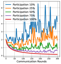
(a) Train loss.

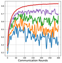
(b) Test accuracy.

​​​

Figure 1: “Dual drift” issue of the federated primal dual method under different participation ratios. When the participation ratio is low, dual drift introduces a very large variance, yielding divergence.

However, as studies go further, a series of problems of federated primal dual methods in the experiments are also exposed. Sensitivity to hyperparameters and fluctuations affected by the large scale makes it extremely unstable in practice, especially in the partial participation manner which is one of the most important concerns in FL. Specifically, primal dual methods successfully solve the problems by alternately updating each primal variable and each dual variable. When it is grafted onto the partial participation training in FL, most clients will remain inactive for a long time, which means most of the dual variables will be stagnant and very outdated in the training. As the training process continues, when one long-term inactive client is reactivated to participate in training, the solving process of its local subproblem will become extremely unstable due to excessive differences between the primal and dual variables, and sometimes even fail. We call this a “dual drift” problem, which is also one of the most formidable challenges in practice in FL. In Fig.1, we clearly show how the “dual drift” deteriorates as the participation ratio decreases. This instability seriously hinders the application of such methods.

To efficiently expand the primal dual methods to partial participation scenarios while enhancing the training stability in practice, and further alleviate the “dual drift” problem, we propose a novel algorithm, named Aligned Federated Primal Dual (A-FedPD), which constructs the virtual dual updates for those unparticipated clients per communication round to align with primal variables. Concretely, after each communication round, we first aggregate the local solutions received from active clients as the unbiased approximation of the local solution of those unparticipated clients. Then we provide a virtual update on the dual variables to align with the primal variable in the training. Updating errors for dual variables will be diminished as global consensus is achieved. The proposed A-FedPD method enables unparticipated clients to keep up-to-date, which approximates the quasi-full-participation training, which can efficiently alleviate the “dual drift” in practice.

Furthermore, we provide a comprehensive analysis of the optimization and generalization efficiency of the proposed A-FedPD method, which also could be easily extended to the whole federated primal dual family. On smooth non-convex objectives, compared with the vanilla FedAvg method, the A-FedPD could achieve a fast $\mathcal{O}(1/T)$ convergence rate which maintains consistent with SOTA federated primal dual methods. Moreover, it could support longer local training without affecting stability. Under the same training costs, the A-FedPD method achieves less generalization error. We conduct extensive experiments to validate its efficiency across several general federated setups. We also test a simple variant to show its good scalability incorporated with other novel techniques in FL.

We summarize our major contributions as follows:

• We review the development of federated primal dual family and point out one of its most formidable challenges in the practical application in FL, which is summarized as the “dual drift” problem in this paper.

• We propose a novel A-FedPD method to alleviate the “dual drift”, which constructs the virtual update for dual variables of those unparticipated clients to align with primal variables.

• We provide a comprehensive analysis of the optimization and generalization efficiency of A-FedPD. It could achieve a fast convergence rate and a lower generalization error bound than the vanilla FedAvg method.

• Extensive experiments are conducted to validate the performance of the A-FedPD method. Furthermore, we test a simple variant of it to show its good scalability.

2 Related Work

Federated primal average. Since McMahan et al. (2017) propose the FedAvg paradigm, a lot of primal average-based methods are learned to enhance its performance. Most of them target strengthening global consistency and alleviating the “client drift” problem (Karimireddy et al., 2020). Li et al. (2020) propose to adopt proxy terms to control local updates. Karimireddy et al. (2020) propose the variance reduction version to handle the biases in the primal average. Similar implementations include (Dieuleveut et al., 2021; Jhunjhunwala et al., 2022). Moreover, momentum-based methods are also popular for correcting local biases. Ozfatura et al. (2021); Xu et al. (2021) propose to adopt the global consistency controller in the local training to force a high consensus. Remedios et al. (2020) expand the local momentum to achieve higher accuracy in the training. Similarly, Wang et al. (2019); Kim et al. (2022) incorporate the global momentum which could further improve its performance. Wang et al. (2020b) tackle the local inconsistency and utilize the weighted primal average to balance different clients with different computing power. Based on this, Horváth et al. (2022) further select the important clients set to balance the training trends under different heterogeneous datasets. Liu et al. (2023) summarize the inertial momentum implementation which could achieve a more stable result. Qu et al. (2022) utilize the Sharpeness Aware Minimization (SAM) (Foret et al., 2020) to make the loss landscape smooth with higher generalization performance. Then Caldarola et al. (2022, 2023) propose to improve its stability via Adaptive SAM and window-based model averaging. In summary, Federated primal average methods focus on alleviating the local inconsistency caused by “client drift” (Malinovskiy et al., 2020; Wang et al., 2020a; Charles and Konečnỳ, 2021). However, as analyzed by Durmus et al. (2021), the federated primal dual methods will regularize the local objective gradually close to global consensus by dynamically adjusting the dual variables. This allows “client drift” to be effectively translated into a dual consistency problem on cross-silo devices.

Convex optimization of federated primal dual. The primal-dual method was originally proposed to solve convex optimization problems and achieved high theoretical performance. In the FL setups, this method has also made significant advancements. Grudzień et al. (2023a) compute inexactly a proximity operator to work as a variant of primal dual methods. Another technique is loopless instead of an inner loop of local steps. Mishchenko et al. (2022) propose the Scaffnew method to achieve the higher optimization efficiency, which is interpreted as a variant of primal dual approach (Condat and Richtárik, 2022). These techniques can also be easily combined with existing efficient communication methods, e.g. compression and quantization (Grudzień et al., 2023b; Condat et al., 2023).

Non-convex optimization of federated primal dual. Since Tran Dinh et al. (2021) adopt the Randomized Douglas-Rachford Splitting, which unblocks the study of the important branch of utilizing primal dual methods in FL (Pathak and Wainwright, 2020). With further exploration of Zhang et al. (2021), federated primal dual methods are proven to achieve the fast convergence rate. Yuan et al. (2021) learn the composite optimization via a primal dual method in FL. Meanwhile, Sarcheshmehpour et al. (2021) empower its potential on the undirected empirical graph. Shen et al. (2021) also study an agnostic approach under class imbalance targets. Then, Gong et al. (2022); Wang et al. (2022) expand its theoretical analysis to the partial participation scenarios with global regularization. Durmus et al. (2021) improve its implementation by introducing the global dual variable. Moreover, Zhou and Li (2023) learn the effect of subproblem precision on training efficiency. Sun et al. (2023b, a) incorporate it with the SAM to achieve a higher generalization efficiency. Niu and Wei (2023) propose hybrid primal dual updates with both first-order and second-order optimization. Wang et al. (2023) propose a variance reduction variant to further improve the training efficiency. Li et al. (2023a) expand it to a decentralized approach, which could achieve comparable performance in the centralized. Tyou et al. (2023) propose a localized primal dual approach for FL training. Li et al. (2023b) further explore its efficiency on the specific non-convex objectives with non-smooth regularization. Current researches reveal the great application value of the primal dual methods in FL. However, most of them still face the serious “dual drift” problem at low participation ratios. Our improvements further alleviate this issue and make the federated primal dual methods perform more stably in the FL community.

3 Methodology

Table 1: Notations adopted in this paper.

Symbol	Notations
$\mathcal{C}$ / $C$	client set / size of client set
$\mathcal{P}$ / $P$	active client set / size of active client set
$\mathcal{S}_{i}$ / $S$	local dataset / size of local dataset
$\theta$ / $\theta_{i}$	global parameters / local parameters
$\lambda$ / $\lambda_{i}$	global dual parameters / local dual parameters
$T$ / $t$	training round / index of training round
$K$ / $k$	local interval / index of local interval
$\rho$	proxy coefficient

We first review the primal dual methods in FL and demonstrate the “dual drift” issue. Then, we demonstrate the A-FedPD approach to eliminate the “dual drift” challenge. Notations are stated in Table 1. Other symbols are defined when they are first introduced. We denote $\mathbb{R}$ as the real set and $\mathbb{E}$ as the expectation in the corresponding probability space. Other notations are defined as first stated.

3.1 Preliminaries

Setups. In the general and classical federated frameworks, we usually consider the general objective as a finite-sum minimization problem $F(\theta):\mathbb{R}^{d}\rightarrow\mathbb{R}$,

$$\small\min_{\theta}F(\theta)=\frac{1}{C}\sum_{i\in\mathcal{C}}F_{i}(\theta),\quad F_{i}(\theta)\triangleq\mathbb{E}_{\xi\sim\mathcal{D}_{i}}f_{i}(\theta,\xi).$$ (1)

In each client, there exists a local private data set $\mathcal{S}_{i}$ which is considered a uniform sampling set of the distribution $\mathcal{D}_{i}$. In FL setups, $\mathcal{D}_{i}$ is unknown to others for the privacy protection mechanism. Therefore, we usually consider the local Empirical Risk Minimization (ERM) as:

$$\small\min_{\theta}f(\theta)=\frac{1}{C}\sum_{i\in\mathcal{C}}f_{i}(\theta),\quad f_{i}(\theta)\triangleq\frac{1}{S}\sum_{\xi\in\mathcal{S}_{i}}f_{i}(\theta,\xi).$$ (2)

Our desired optimal solution is $\theta^{\star}=\arg\min F(\theta)$. However, we can only approximate it on the limited dataset as $\theta_{\mathcal{S}}^{\star}=\arg\min f(\theta)$, which spontaneously introduces the unavoidable biases on its generalization performance. This is one of the main concerns in the field of the current machine learning community. Motivated by this imminent challenge, we conduct a comprehensive study on the performance of primal dual-based algorithms in FL and further propose an improvement to enhance its generalization efficiency and stability performance.

3.2 Primal Dual-family in FL

Primal Dual methods optimize the global objective by decomposing it into several subproblems and iteratively updating local variables incorporated by Lagrangian multipliers (Boyd et al., 2011), which gives it a unique position in solving FL problems. Due to local data privacy, we have to split the global task into several local tasks for optimization on their private dataset. This similarity also provides an adequate foundation for their applications in the FL community. A lot of studies extend it to the general FL framework and achieve considerable success.

We follow studies (Zhang et al., 2021; Durmus et al., 2021; Wang et al., 2022; Gong et al., 2022; Sun et al., 2023b; Zhou and Li, 2023; Sun et al., 2023a; Fan et al., 2023; Zhang et al., 2024) to summarize the original objective Eq.(2) as the global consensus reformulation:

$$\small\min_{\theta,\theta_{i}}\frac{1}{C}\sum_{i\in\mathcal{C}}f_{i}(\theta_{i}),\quad\text{s.t.}\quad\theta_{i}=\theta,\quad\forall i\in\mathcal{C}.$$ (3)

By relaxing equality constraints $\theta_{i}=\theta$, Eq.(3) is separable across different local clients. Wang et al. (2022) demonstrate the difference between the solution on the primal problem and dual problem in detail and confirm the equivalence of these two cases in FL. By penalizing the constraint on the local objective $f_{i}$, we can define the augmented Lagrangian function associated with Eq.(3) as:

$$\small\mathcal{L}(\theta_{i},\theta,\lambda_{i})=\frac{1}{C}\sum_{i\in\mathcal{C}}\left[f_{i}(\theta_{i})\!+\!\langle\lambda_{i},\theta_{i}\!-\!\theta\rangle\!+\!\frac{\rho}{2}\|\theta_{i}\!-\!\theta\|^{2}\right],$$ (4)

where $\rho$ denotes the penalty coefficient. To train the global model, each local client should first minimize the local augmented Lagrangian function and solve for local parameters. Based on updated local parameters, we then update the dual variable to align the Lagrangian function with the consensus constraints. Finally, we minimize the augmented Lagrangian function and solve for the consensus. Objective Eq.(3) could be solved after multiple alternating updates as:

$$\small\begin{cases}\ \theta_{i}^{t+1}&=\quad\arg\min_{\theta_{i}}\ \mathcal{L}(\theta_{i}^{t},\theta^{t},\lambda_{i}^{t})\quad i\in\mathcal{C},\\ \ \lambda_{i}^{t+1}&=\quad\lambda_{i}^{t}+\rho(\theta_{i}^{t+1}-\theta^{t}),\\ \ \theta^{t+1}&=\quad\frac{1}{C}\sum_{i\in\mathcal{C}}(\theta_{i}^{t+1}+\frac{1}{\rho}\lambda_{i}^{t+1}).\\ \end{cases}$$ (5)

We then review the classical federated primal dual methods.

FedPD. Zhang et al. (2021) propose a general federated framework from the primal-dual optimization perspective which can be directly summarized as Eq.(5). As an underlying method in the federated primal dual-family, it requires all local clients to participate in the training per round, which also significantly reduces communication efficiency.

FedADMM. Wang et al. (2022) extend the theory of the primal-dual optimization in FL and prove the equivalence between FedDR (Tran Dinh et al., 2021) and FedADMM. Furthermore, it considers the complete format of composite objective $f(\theta_{i})+g(\theta)$. To optimize the composite objective, after the iterations of Eq.(5), it additionally solves the proximal step on the function $g(\theta)$:

$$\small\begin{cases}\ \theta_{i}^{t+1}&=\quad\arg\min_{\theta_{i}}\ \mathcal{L}(\theta_{i}^{t},\theta^{t},\lambda_{i}^{t})+g(\theta^{t})\quad i\in\mathcal{P}^{t},\\ \ \lambda_{i}^{t+1}&=\quad\lambda_{i}^{t}+\rho(\theta_{i}^{t+1}-\theta^{t}),\\ \ \overline{\theta}^{t+1}&=\quad\frac{1}{P}\sum_{i\in\mathcal{P}^{t}}(\theta_{i}^{t+1}+\frac{1}{\rho}\lambda_{i}^{t+1}),\\ \ \theta^{t+1}&=\quad\arg\min g(\theta^{t})+\frac{1}{2\rho}\|\theta^{t}-\overline{\theta}^{t+1}\|^{2}.\\ \end{cases}$$ (6)

FedADMM introduces a more general update with the regularization term $g(\theta)$ and supports the partial participation training mechanism, which also brings a great application value of primal-dual methods to the FL community. When $g(\cdot)\equiv 0$, it degrades to the partial FedPD by $\theta^{t+1}=\overline{\theta}^{t+1}$. When $\mathcal{P}^{t}\neq\mathcal{C}$, “dual drift” brings great distress for training.

FedDyn. Durmus et al. (2021) utilize the insight of primal-dual optimization to introduce a dynamic regularization term to solve the local augmented Lagrangian function, which is actually the dual variable in FedADMM. Differently, they propose a global dual variable $\lambda^{t}$ to update global parameters $\theta^{t}$ instead of only active local dual variables $\lambda_{i}^{t}$ ($i\in\mathcal{P}^{t}$):

$$\small\begin{cases}\ \theta_{i}^{t+1}&=\quad\arg\min_{\theta_{i}}\ \mathcal{L}(\theta_{i}^{t},\theta^{t},\lambda_{i}^{t})\quad i\in\mathcal{P}^{t},\\ \ \lambda_{i}^{t+1}&=\quad\lambda_{i}^{t}+\rho(\theta_{i}^{t+1}-\theta^{t}),\\ \ \lambda^{t+1}&=\quad\lambda^{t}+\rho\frac{1}{C}\sum_{i\in\mathcal{P}^{t}}(\theta_{i}^{t+1}-\theta^{t}),\\ \ \theta^{t+1}&=\quad\frac{1}{P}\sum_{i\in\mathcal{P}^{t}}\theta_{i}^{t+1}+\frac{1}{\rho}\lambda^{t}.\\ \end{cases}$$ (7)

Compared with FedADMM, although the global dual variable further corrects the primal parameters, it still hinders the training efficiency, which must rely on the anachronistic historical directions of the local dual variables. Moreover, the global dual variable always updates slowly, which results in consensus constraints that are more difficult to satisfy when solving local subproblems.

Dual drift. Kang et al. (2024) have indicated that the update mismatch between primal and dual variables leads to a ”drift”. Here, we provide a detailed analysis of the key differences caused by this mismatch. When adopting partial participation, each client is activated at a very low probability, especially on a large scale of edged devices, which widely leads to very high hysteresis between global parameters $\theta$ and local dual variable $\lambda_{i}$. For instance, at round $t$, we select a subset $\mathcal{P}^{t}$ to participate in current training and then update the global parameters by $\theta^{t+1}=\arg\min_{\theta}\ \mathcal{L}(\theta_{i}^{t+1},\theta^{t},\lambda_{i}^{t})$ for $i\in\mathcal{P}^{t}$. Then at round $t+1$, when a client $i\notin\{\mathcal{P}^{\tau}\}_{\tau=t_{0}+1}^{t}$ $(t_{0}\ll t)$ that has not been involved in training for a long time is activated, its local dual variable $\lambda_{i}^{t_{0}}$ may severely mismatch the current global parameters $\theta^{t}$. This triggers that the local subproblem $\mathcal{L}(\theta_{i}^{t+1},\theta^{t+1},\lambda_{i}^{t_{0}})$ fail to be optimized properly and even become completely distorted in extreme scenarios, yielding a “dual drift” issue.

3.3 A-FedPD Method

As introduced in the last part, “dual drift” problem usually results in the unstable optimization of each local subproblem under partial participation. To further mitigate the negative effects of dual drift problems and improve the training efficiency, we propose a novel A-FedPD method (see Algorithm 1), which aligns the virtual dual variables of unparticipated clients via global average models.

Specifically, we solve dual variables for unified management and distribution. At round $t$, we select an active client set $\mathcal{P}^{t}$ and send the corresponding variables to each active client. Then local client solves the subproblem with $K$ stochastic gradient descent steps and sends the last state $\theta_{i,K}^{t}$ back to the global server. On the global server, it first aggregates the updated parameters as $\overline{\theta}^{t+1}$. Then it performs the updates of the dual variables. For each active client $i\in\mathcal{P}^{t}$, it equally updates the local dual variable as vanilla FedPD. For the unparticipated clients $i\notin\mathcal{P}^{t}$, they update the virtual dual variable with the aggregated parameters $\overline{\theta}^{t+1}$. Finally, we can update the global model with the aggregated parameters and averaged dual variables. Since each client virtually updates, we can directly use the global average as the output. Repeat this training process for a total of $T$ communication rounds to output the final global average model.

Algorithm 1 A-FedPD Algorithm

0:  $\theta^{0}$, $\theta_{i}^{0}$, $T$, $K$, $\lambda_{i}^{0}$, $\rho$

0:  global average model

1:  Initialization : $\theta_{i}^{0}=\theta^{0}$, $\lambda_{i}^{0}=0$.

2:  for $t=0,1,2,\cdots,T-1$ do

3:     randomly select active clients set $\mathcal{P}^{t}$ from $\mathcal{C}$

4:     for client $i\in\mathcal{P}^{t}$ in parallel do

5:        receive $\lambda_{i}^{t},\theta^{t}$ from the global server

6:        $\theta_{i}^{t+1}=\textit{LocalTrain}(\lambda_{i}^{t},\theta^{t},\eta^{t},K)$

7:        send $\theta_{i}^{t+1}$ to the global server

8:     end for

9:     $\overline{\theta}^{t+1}=\frac{1}{P}\sum_{i\in\mathcal{P}^{t}}\theta_{i}^{t+1}$

10:     $\lambda_{i}^{t+1}=\textit{D-Update}(\lambda_{i}^{t},\theta^{t},\theta_{i}^{t+1},\overline{\theta}^{t+1},\mathcal{P}^{t})$

11:     $\overline{\lambda}^{t+1}=\frac{1}{C}\sum_{i\in\mathcal{C}}\lambda_{i}^{t+1}$

12:     $\theta^{t+1}=\overline{\theta}^{t+1}+\frac{1}{\rho}\overline{\lambda}^{t+1}$

13:  end for

14:  return global average model

$\diamondsuit$ LocalTrain: (Optimize Eq.(4))

0:  $\lambda_{i}^{t}$, $\theta^{t}$, $\eta^{t}$, $K$

0:  $\theta_{i,K}^{t}$

1:  for $k=0,1,2,\cdots,K-1$ do

2:     calculate the stochastic gradient $g_{i,k}^{t}$

3:     $\theta_{i,k+1}^{t}=\theta_{i,k}^{t}-\eta^{t}(g_{i,k}^{t}+\lambda_{i}^{t}+\rho(\theta_{i,k}^{t}-\theta^{t}))$

4:  end for

$\diamondsuit$ D-Update: (update dual variables)

0:  $\lambda_{i}^{t},\theta^{t},\theta_{i}^{t+1},\overline{\theta}^{t+1},\mathcal{P}^{t}$

0:  $\lambda_{i}^{t+1}$

1:  if $i\in\mathcal{P}^{t}$ then

2:     $\lambda_{i}^{t+1}=\lambda_{i}^{t}+\rho_{t}(\theta_{i}^{t+1}-\theta^{t})$

3:  else

4:     $\lambda_{i}^{t+1}=\lambda_{i}^{t}+\rho_{t}(\overline{\theta}^{t+1}-\theta^{t})$

5:  end if

Because of the central storage and management of the dual variables on the global server, it significantly reduces storage requirements for lightweight-edged devices, i.e., mobile phones. For the unparticipated clients, we use their unbiased estimations $\mathbb{E}\left[w_{i}^{t+1}|\ w^{t}\right]=\mathbb{E}_{\mathcal{P}^{t}}\left[\frac{1}{P}\sum_{i\in\mathcal{P}^{t}}w_{i}^{t+1}|\ w^{t}\right]$ to construct the virtual dual update, which maintains a continuous update of local dual variables. For the global averaged dual variable $\overline{\lambda}$, we can reformulate its update as $\overline{\lambda}^{t+1}=\overline{\lambda}^{t}+\rho(\overline{\theta}^{t+1}-\theta^{t})$ which also could be approximated as a virtual all participation case. This efficiently alleviates the dual drift between $\theta^{t}$ and $\lambda_{i}^{t}$ and also ensures fast iteration of the global dual variable in the training, which constitutes an efficient federated framework.

4 Theoretical Analysis

In this part, we mainly introduce the theoretical analysis of the optimization and generalization efficiency of our proposed A-FedPD method. We first introduce the assumptions adopted in our proofs. Optimization analysis is stated in Sec.4.1 and generalization analysis is stated in Sec.4.2.

Assumption 1 (Smoothness).

The local function $f_{i}(\cdot)$ satisfies the $L$-smoothness property, i.e., $\|\nabla f_{i}(\theta_{1})-\nabla f_{i}(\theta_{2})\|\leq L\|\theta_{1}-\theta_{2}\|$.

Assumption 2 (Lipschitz continuity).

For $\forall\ \theta_{1},\theta_{2}\in\mathbb{R}^{d}$, the global function $f(\cdot)$ satisfies the Lipschitz-continuity, i.e., $\|f(\theta_{1})-f(\theta_{2})\|\leq G\|\theta_{1}-\theta_{2}\|$.

Optimization analysis only adopts Assumption 1. Generalization analysis adopts both assumptions that were followed from the previous work on analyzing the stability (Hardt et al., 2016; Lei and Ying, 2020; Zhou et al., 2021; Sun et al., 2023e, d, c). Moreover, we consider that the minimization of each local Lagrangian problem achieves the $\epsilon$-inexact solution during each local training process, i.e. $\|\nabla\mathcal{L}_{i}\|^{2}\leq\epsilon$ (Zhang et al., 2021; Li et al., 2023a; Gong et al., 2022; Wang et al., 2022). This consideration is more aligned with the practical scenarios encountered in the empirical studies for non-convex optimization. In fact, it is precisely because the errors from local inexact solutions can be excessively large that the dual drift problem is further exacerbated.

4.1 Optimization

In this part, we introduce the convergence analysis of the proposed A-FedPD method.

Theorem 1.

Let non-convex objective $f$ satisfies Assumption 1, let $\rho$ be selected as a non-zero positive constant, $\{\overline{\theta}^{t}\}_{t=0}^{T}$ sequence generated by algorithm 1 satisfies:

$$\small\frac{1}{T}\sum_{t=1}^{T}\mathbb{E}\|\nabla f(\overline{\theta}^{t})\|^{2}\leq\frac{\rho\left[f(\overline{\theta}^{1})-f^{\star}\right]+R_{0}}{T}+\mathcal{O}\left(\epsilon\right),$$ (8)

where $f^{\star}$ is the optimum and $R_{0}=\frac{1}{C}\sum_{i\in\mathcal{C}}\mathbb{E}_{t}\|\theta_{i}^{1}-\theta^{0}\|^{2}$ is the first local training volumes.

Remark 1.1.

To achieve the $\epsilon$ error, the A-FedPD requires $\mathcal{O}(\epsilon^{-1})$ rounds, yielding $\mathcal{O}(1/T)$ convergence rate. Concretely, the federated primal dual methods can locally train more and communicate less, which empowers it a great potential in the applications. Our analysis is consistent with the previous understandings (Zhang et al., 2021; Durmus et al., 2021; Gong et al., 2022; Li et al., 2023a).

Remark 1.2.

Generally, the federated primal-dual methods require a long local interval. Zhang et al. (2021); Gong et al. (2022); Wang et al. (2022) have summarized the corresponding selections of $K$ for different local optimizers. To complete the analysis, we just list a general selection of the local interval $K$. Specifically, to achieve the $\epsilon$ error, local interval $K$ of A-FedPD can be selected as $\mathcal{O}(\epsilon^{-1})$ with total $\mathcal{O}(\epsilon^{-2})$ sample complexity in the training. Due to the page limitation, we state more discussions in the Appendix B.2.2.

4.2 Generalization

In this part, we explore the efficiency of A-FedPD from the stability and generalization perspective, which could also be extended to the common primal dual-family in the federated learning community. We first introduce the setups and assumptions and then demonstrate the main theorem and discussions.

Setups. To understand the stability and generalization efficiency, we follow Hardt et al. (2016); Lei and Ying (2020); Zhou et al. (2021); Sun et al. (2023e) to adopt the uniform stability analysis to measure its error bound. To learn the generalization gap $\mathbb{E}\left[F(\theta^{T})-f(\theta^{T})\right]$ where $\theta^{T}$ is generated by a stochastic algorithm, we could study its stability gaps. We consider a joint client set $\mathcal{C}$ (union dataset) for training. Each client $i$ has a private dataset $\mathcal{S}_{i}$ with total $S$ samples which are sampled from the unknown distribution $\mathcal{D}_{i}$. To explore the stability gaps, we construct a mirror dataset $\hat{\mathcal{C}}$ that there is at most one different data sample from the raw dataset $\mathcal{C}$. Let $\theta^{T}$ and $\hat{\theta}^{T}$ be two models trained on $\mathcal{C}$ and $\hat{\mathcal{C}}$ respectively. Therefore, the generalization of a uniformly stable method satisfies:

$$\small\mathbb{E}\left[|F(\theta^{T})-f(\theta^{T})|\right]\leq\sup_{\xi}\mathbb{E}\left[|f(\theta^{T},\xi)-f(\hat{\theta}^{T},\xi)|\right]\leq\varepsilon.$$ (9)

Key properties. From the local training, we can first upper bound the local stability. To compare the difference between vanilla SGD updates and primal dual-family updates, we can reformulate them:

$$\small\begin{cases}\theta_{i,k+1}^{t}-\theta^{t}&=(\theta_{i,k}^{t}-\theta^{t})+\eta^{t}g_{i,k}^{t},\\ \theta_{i,k+1}^{t}-\theta^{t}&=(1-\eta^{t}\rho)(\theta_{i,k}^{t}-\theta^{t})+\eta^{t}(g_{i,k}^{t}+\lambda_{i}).\end{cases}$$ (10)

The above update is for vanilla FedAvg and the below update is for primal dual-family. When the dual variables are ignored, local update $\theta_{i,k}^{t}-\theta^{t}$ in primal dual could be considered as a stable decayed sequence with $1-\eta^{t}\rho$ that has a constant upper bound. Based on this, we can provide a tighter generalization error bound for the primal dual-family methods in FL than the vanilla FedAvg method.

Theorem 2.

Let non-convex objective $f$ satisfies Assumption 1 and 2 and $H=\sup_{\theta,\xi}f(\theta,\xi)$, after $T$ communication rounds training with Algorithm 1, the generalization error bound achieves:

$$\small\mathbb{E}\left[F(\theta^{T})-f(\theta^{T})\right]\leq\frac{\kappa_{c}}{CS}\left(HPT\right)^{\frac{\mu L}{1+\mu L}},$$ (11)

where $\mu$ is a constant related to the learning rate and $\kappa_{c}=4\left(G^{2}/L\right)^{\frac{1}{1+\mu L}}$ is a constant.

Remark 2.1.

We assume that the total number of data samples participating in the training is $CS$ and the total iterations of the training are $KT$. Hardt et al. (2016) prove that on non-convex objectives, vanilla SGD method achieves $\mathcal{O}((TK)^{\frac{\mu L}{1+\mu L}}/CS)$ error bound. Compared with SGD, FL adopts the cyclical local training and partial participation mechanism which further increases the stability error. Sun et al. (2023d) learn a fast rate on sample size as $\mathcal{O}((PKT)^{\frac{\mu L}{1+\mu L}}/CS)$ under the Lipschitz assumption only. However, primal dual-family can achieve faster rate $\mathcal{O}((PT)^{\frac{\mu L}{1+\mu L}}/CS)$ in FL, which is due to the stable iterations in Eq.(10). It guarantees that the local training could be bounded in a constant order even under the fixed learning rate. From the local training perspective, primal dual-family in FL can support a very long local interval $K$ without losing stability. This property is also proven in its optimization progress, that the primal dual-family could adopt a larger local interval to accelerate the training and reduce the communication rounds. In general training, especially in situations where communication bandwidth is limited and frequent communication is not possible, the primal dual-family in FL could achieve a more stable result than the general methods. Our analysis further confirms its good adaptivity in FL. Due to page limitation, we summarize some recent results of the generalization error bound in Appendix B.3.2.

5 Experiments

Table 2: Test accuracy on the CIFAR-10 / 100 dataset. We fix the total client $C=100$ and $P=10$ under training local 50 iterations. We test 3 setups of IID, Dir-1.0, and Dir-0.1 on each dataset. Each group is tested on LeNet (upper portion) and ResNet-18 (lower portion) models. Each results are tested with 4 different random seeds. “$-$” means can not stably converge. “Family” distinguishes whether the algorithm is a primal method (P) or a primal dual method (PD) and “Local Opt” distinguishes whether the algorithm adopts SGD-based or SAM-based local optimizer.

			CIFAR-10			CIFAR-100
	Family	Local Opt	IID	Dir-1.0	Dir-0.1	IID	Dir-1.0	Dir-0.1
FedAvg	P	SGD	$\text{81.87}_{\pm.12}$	$\text{80.58}_{\pm.15}$	$\text{75.57}_{\pm.27}$	$\text{40.11}_{\pm.17}$	$\text{39.65}_{\pm.07}$	$\text{38.37}_{\pm.14}$
FedCM	P	SGD	$\text{80.34}_{\pm.14}$	$\text{79.31}_{\pm.33}$	$\text{72.89}_{\pm.37}$	$\text{43.33}_{\pm.13}$	$\text{42.35}_{\pm.25}$	$\text{37.11}_{\pm.51}$
SCAFFOLD	P	SGD	$\text{84.25}_{\pm.16}$	$\text{83.61}_{\pm.14}$	$\text{78.66}_{\pm.29}$	$\text{49.65}_{\pm.06}$	$\text{49.11}_{\pm.14}$	$\text{46.36}_{\pm.30}$
FedSAM	P	SAM	$\text{83.22}_{\pm.09}$	$\text{81.94}_{\pm.13}$	$\text{77.41}_{\pm.36}$	$\text{43.02}_{\pm.09}$	$\text{42.83}_{\pm.29}$	$\text{42.29}_{\pm.23}$
FedDyn	PD	SGD	$\text{84.49}_{\pm.22}$	$\text{84.20}_{\pm.14}$	$\text{79.51}_{\pm.13}$	$\text{50.27}_{\pm.11}$	$\text{49.64}_{\pm.21}$	$\text{46.30}_{\pm.26}$
FedSpeed	PD	SAM	$\text{86.01}_{\pm.18}$	$\text{85.11}_{\pm.21}$	$\text{80.86}_{\pm.18}$	$\text{54.01}_{\pm.15}$	$\text{53.45}_{\pm.23}$	$\text{51.28}_{\pm.18}$
A-FedPD	PD	SGD	$\text{85.31}_{\pm.14}$	$\text{84.94}_{\pm.13}$	$\text{80.28}_{\pm.20}$	$\text{51.41}_{\pm.15}$	$\text{51.17}_{\pm.17}$	$\text{48.15}_{\pm.28}$
A-FedPDSAM	PD	SAM	$\textbf{86.47}_{\pm.18}$	$\textbf{85.90}_{\pm.29}$	$\textbf{81.96}_{\pm.19}$	$\textbf{55.56}_{\pm.27}$	$\textbf{54.62}_{\pm.16}$	$\textbf{53.15}_{\pm.19}$
FedAvg	P	SGD	$\text{81.67}_{\pm.21}$	$\text{80.94}_{\pm.17}$	$\text{76.24}_{\pm.35}$	$\text{44.68}_{\pm.21}$	$\text{44.27}_{\pm.25}$	$\text{41.64}_{\pm.27}$
FedCM	P	SGD	$\text{84.22}_{\pm.17}$	$\text{82.85}_{\pm.21}$	$\text{76.93}_{\pm.32}$	$\text{50.04}_{\pm.16}$	$\text{48.66}_{\pm.28}$	$\text{44.07}_{\pm.30}$
SCAFFOLD	P	SGD	$\text{84.31}_{\pm.14}$	$\text{83.70}_{\pm.11}$	$\text{78.70}_{\pm.21}$	$\text{50.69}_{\pm.21}$	$\text{50.28}_{\pm.21}$	$\text{47.12}_{\pm.34}$
FedSAM	P	SAM	$\text{83.79}_{\pm.28}$	$\text{82.58}_{\pm.19}$	$\text{77.83}_{\pm.27}$	$\text{48.66}_{\pm.29}$	$\text{48.42}_{\pm.19}$	$\text{45.03}_{\pm.22}$
FedDyn	PD	SGD	$\text{83.71}_{\pm.26}$	$\text{82.66}_{\pm.15}$	$\text{79.44}_{\pm.25}$	$-$	$-$	$-$
FedSpeed	PD	SAM	$\text{86.90}_{\pm.18}$	$\text{85.92}_{\pm.24}$	$\text{81.47}_{\pm.19}$	$\text{53.22}_{\pm.28}$	$\text{52.75}_{\pm.16}$	$\text{49.66}_{\pm.13}$
A-FedPD	PD	SGD	$\text{85.11}_{\pm.12}$	$\text{84.33}_{\pm.16}$	$\text{81.05}_{\pm.28}$	$\text{48.15}_{\pm.22}$	$\text{48.02}_{\pm.29}$	$\text{46.24}_{\pm.26}$
A-FedPDSAM	PD	SAM	$\textbf{87.44}_{\pm.13}$	$\textbf{86.46}_{\pm.25}$	$\textbf{82.48}_{\pm.21}$	$\textbf{55.30}_{\pm.23}$	$\textbf{53.49}_{\pm.17}$	$\textbf{50.31}_{\pm.23}$

In this section, we introduce the experiments conducted to validate the efficiency of our proposed A-FedPD and a variant A-FedPDSAM (see details in Appendix A.1). We first introduce experimental setups and benchmarks, and then we show the empirical studies.

Backbones and Datasets. In our experiments, we adopt LeNet LeCun et al. (1998) and ResNet He et al. (2016) as backbones. We follow previous work to test the performance of benchmarks on the CIFAR-10 / 100 dataset Krizhevsky et al. (2009). We introduce the heterogeneity to split the raw dataset to local clients with independent Dirichlet distribution Hsu et al. (2019) controlled by a concentration parameter. In our setups, we mainly test the performance of the IID, Dir-1.0, and Dir-0.1 splitting. The Dir-1.0 represents the low heterogeneity and Dir-0.1 represents the high heterogeneity. We also adopt the sampling with replacement to further enhance the heterogeneity.

Setups. We test the accuracy experiments on $C=100$ and $P/C=10\%$, which is also the most popular setup in the FL community. In the comparison experiments, we test the participated ratio $P/C=\left[5\%,10\%,20\%,50\%,80\%,100\%\right]$ and local interval $K=\left[10,20,50,100,200\right]$ respectively. In each setup, for a fair comparison, we freeze the most of hyperparameters for all methods. We fix total communication rounds $T=800$ except for the ablation studies.

Baselines. FedAvg (McMahan et al., 2017) is the fundamental paradigm in FL scenarios. FedCM (Xu et al., 2021), SCAFFOLD (Karimireddy et al., 2020) and FedSAM (Qu et al., 2022) are three classical SOTA methods in the federated primal average family. FedDyn (Durmus et al., 2021) and FedSpeed Sun et al. (2023b) are relatively stable federated primal dual methods. A more detailed introduction of these methods is presented in Table 2, including the family-basis and local optimizer.

5.1 Experiments

In this part, we introduce the phenomena observed in our empirical studies. We primarily investigated performance comparisons, including settings with different participation rates, various local intervals, and different numbers of communication rounds. Then we report the comparison of wall-clock time.

Performance Comparison. Table 2 shows the test accuracy on CIFAR-10 / 100 dataset. The vanilla FedAvg provides the standard bars as the baseline. In the federated primal average methods, The FedCM is not stable enough and is largely affected by different backbones, which is caused by the forced consistency momentum and may introduce very large biases. SCAFFOLD and FedSAM performs well. However, both are less than the primal dual-based methods. In summary, SCAFFOLD is on average 3.2% lower than FedSpeed. As heterogeneity increases, SCAFFOLD drops on average about 5.6% on CIFAR-10 and 3.43% on CIFAR-100. In the federated primal dual methods, we can clearly see that FedDyn is not stable in the training. It performs well on the LeNet, which could achieve at least 1% improvements than SCAFFOLD. However, when the task becomes difficult, i.e., ResNet-18 on CIFAR-100, its accuracy is affected by the “dual drift” and drops quickly. To maintain stability, we have to select some weak coefficients to stabilize it and finally get a lower accuracy. Our proposed A-FedPD could efficiently alleviate the negative impacts of the “dual drift”. It performs about on average 0.8% higher than FedDyn on the CIFAR-10 dataset. When FedDyn has to compromise the hyperparameters and becomes extremely unstable on ResNet-18 on the CIFAR-100 dataset, A-FedPD still performs stably. It’s also very scalable. When we introduce the SAM optimizer to replace the vanilla SGD, it could achieve higher performance.

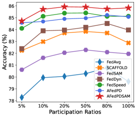
(a) Different Participation Ratios.

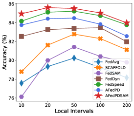
(b) Different Local Intervals.

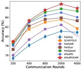
(c) Different Rounds.

​​​ ​​​

Figure 2: Test of the proposed A-FedPD method on setups of different participation ratios, different local intervals, and different rounds. In these experiments, we fix the total training data samples and total training iterations and then learn their variation trends.

Different Participation Ratios. In this part we compare the sensitivity to the participation ratios. In each setup, we fix the scale as 100 and the local interval as 50 iterations. Active ratio is selected from $\left[5\%,10\%,20\%,50\%,80\%,100\%\right]$ as shown in Figure 2 (a). Under frozen hyperparameters, all methods perform well on each selection. The best performance is approximately located in the range of $[20\%,80\%]$. Our proposed methods achieve high efficiency in handling large-scale training, which performs more steadily than other benchmarks across all selections.

Different Local Intervals. In this part we compare the sensitivity to the local intervals. In each setup, we fix the scale as 100 and the participation as 10%. Local interval $K$ is selected from $\left[10,20,50,100,200\right]$ as shown in Figure 2 (b). More local training iterations usually mean more overfitting on the local dataset, which leads to a serious “client drift” issue. All methods will be affected by this and drop accuracy. It is a trade-off in selecting the local interval $K$ to balance both optimization efficiency and generalization stability. Our proposed methods still could achieve the best performance even on the very long local training iterations.

Different Communication Rounds. In this part, we compare the sensitivity to the communication rounds. In each setup, we fix total iterations $TK=40,000$. Communication round $T$ is selected from $\left[200,400,800,2000,4000\right]$ as shown in Figure 2 (c). We always expect the local clients can handle more and communicate less, which will significantly reduce the communication costs. In the experiments, our proposed methods could achieve higher efficiency than the benchmarks. A-FedPD saves about half the communication overhead compared to SCAFFOLD, and about one-third of FedDyn. Under favorable communication bandwidths, they can achieve SOTA performance.

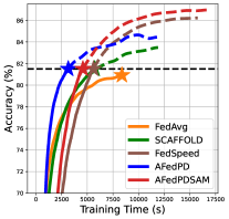
(a) ResNet-18.

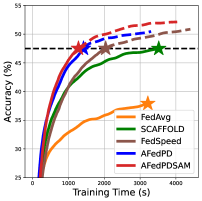
(b) LeNet.

​​​

Figure 3: Wall-clock time test of training process after total of 600 communication rounds.

Wall-clock Time Efficiency. In this part we test the practical wall-clock time comparisons as shown in Figure 3. Though some methods are communication-efficiency, complicated calculations hinder the real efficiency in wall-clock training time. Though FedSpeed and AFedPDSAM perform well at the end, additional calculations per single round make their early-stage competitiveness lower. AFedPD and SCAFFOLD consume fewer time costs, hence achieving better results at the early stage. Without considering training time costs, AFedPDSAM achieves the SOTA results at the end. Detailed comparisons are stated in Sec.A.4.4.

6 Conclusion

In this paper, we first review the development of the federated primal dual methods. Under the exploration of the experiments, we point out a serious challenge that hinders the efficiency of such methods, which is summarized as the “dual drift” problem due to the mismatched primal and dual variables in the partial participation manners. Furthermore, we propose a novel A-FedPD method to alleviate this issue via constructing virtual dual updates for those unparticipated clients. We also theoretically learn its convergence rate and generalization error bound to demonstrate its efficiency. Extensive experiments are conducted to validate its significant performance.

In this part, we introduce the appendix. We introduce the additional experiments in Sec.A including backgrounds, setups, hyperparameters selections, and some figures of experiments. We introduce the theoretical proofs in Sec.B.

Appendix A Additional Experiments

A.1 Benchmarks

We select 6 classical state-of-the-art (SOTA) benchmarks as baselines in our paper, including (a) primal: FedAvg McMahan et al. (2017), SCAFFOLD Karimireddy et al. (2020), FedCM Xu et al. (2021), FedSAM Qu et al. (2022); (b) primal dual: FedADMM Wang et al. (2022), FedDyn Wang et al. (2022), FedSpeed Sun et al. (2023b). We mainly focus on infrastructure improvements instead of combinations of techniques. In the primal group, SCAFFOLD and FedCM alleviate “client drift” via variance reduction and client-level momentum correction respectively. FedSAM introduce the Sharpeness Aware Minimization (SAM) Foret et al. (2020) in vanilla FedAvg to smoothen the loss landscape. In the primal dual group, we select the FedDyn as the stable basis under partial participation. We also show the instability of the vanilla FedADMM to show the negative impacts of the “dual drift”. FedSpeed introduces the SAM in vanilla FedADMM / FedDyn. We also test the variant of SAM version of our proposed A-FedPD method, which is named A-FedPDSAM.

Algorithm 2 A-FedPDSAM Algorithm

0:  $\theta^{0}$, $\theta_{i}^{0}$, $T$, $K$, $\lambda_{i}^{0}$, $\rho$

0:  global average model

1:  Initialization : $\theta_{i}^{0}=\theta^{0}$, $\lambda_{i}^{0}=0$.

2:  for $t=0,1,2,\cdots,T-1$ do

3:     randomly select active clients set $\mathcal{P}^{t}$ from $\mathcal{C}$

4:     for client $i\in\mathcal{P}^{t}$ in parallel do

5:        receive $\lambda_{i}^{t},\theta^{t}$ from the global server

6:        $\theta_{i}^{t+1}=\textit{LocalTrain}(\lambda_{i}^{t},\theta^{t},\eta^{t},K)$

7:        send $\theta_{i}^{t+1}$ to the global server

8:     end for

9:     $\overline{\theta}^{t+1}=\frac{1}{P}\sum_{i\in\mathcal{P}^{t}}\theta_{i}^{t+1}$

10:     $\lambda_{i}^{t+1}=\textit{D-Update}(\lambda_{i}^{t},\theta^{t},\theta_{i}^{t+1},\overline{\theta}^{t+1},\mathcal{P}^{t})$

11:     $\overline{\lambda}^{t+1}=\frac{1}{C}\sum_{i\in\mathcal{C}}\lambda_{i}^{t+1}$

12:     $\theta^{t+1}=\overline{\theta}^{t+1}+\frac{1}{\rho}\overline{\lambda}^{t+1}$

13:  end for

14:  return global average model

$\diamondsuit$ LocalTrain: (Optimize Eq.(4))

0:  $\lambda_{i}^{t}$, $\theta^{t}$, $\eta^{t}$, $K$

0:  $\theta_{i,K}^{t}$

1:  for $k=0,1,2,\cdots,K-1$ do

2:     select a minibatch $\mathcal{B}$

3:     $g_{i,k}^{t}=\nabla f_{i}(\theta_{i,k,t}+\rho\frac{\nabla f_{i}(\theta_{i,k,t},\mathcal{B})}{\|\nabla f_{i}(\theta_{i,k,t},\mathcal{B})\|},\mathcal{B})$

4:     $\theta_{i,k+1}^{t}=\theta_{i,k}^{t}-\eta^{t}(g_{i,k}^{t}+\lambda_{i}^{t}+\rho(\theta_{i,k}^{t}-\theta^{t}))$

5:  end for

$\diamondsuit$ D-Update: (update dual variables)

0:  $\lambda_{i}^{t},\theta^{t},\theta_{i}^{t+1},\overline{\theta}^{t+1},\mathcal{P}^{t}$

0:  $\lambda_{i}^{t+1}$

1:  if $i\in\mathcal{P}^{t}$ then

2:     $\lambda_{i}^{t+1}=\lambda_{i}^{t}+\rho_{t}(\theta_{i}^{t+1}-\theta^{t})$

3:  else

4:     $\lambda_{i}^{t+1}=\lambda_{i}^{t}+\rho_{t}(\overline{\theta}^{t+1}-\theta^{t})$

5:  end if

A.2 Hyperparameters Selection

We first introduce the hyperparameter selections. To fairly compare the efficiency of the benchmarks, we fix the most of hyperparameters, including the initial global learning rate, the initial learning rate, the weight decay coefficient, and the local batchsize. The other hyperparameters are selected properly on a grid search within the valid range. The specific hyperparameters of specific methods are defined in the experiments. We report the corresponding selections of their best performance, which is summarized in the following Table 3.

Table 3: Hyperparameters selections of benchmarks.

	Grid Search	FedAvg	FedCM	SCAFFOLD	FedSAM	FedDyn	FedSpeed
global learning rate	[0.1, 1.0]	1.0
local learning rate	[0.01, 0.1, 1.0]	0.1
weight decay	[0.0001, 0.001, 0.01]	0.001
learning rate decay	[0.995, 0.998, 0.9998, 1]	0.998	0.998	0.998	0.998	0.998 / 1	0.998 / 1
batchsize	[10, 20, 50, 100]	50	50	50	50	20 / 50	50
client-level momentum	[0.05, 0.1, 0.2, 0.5]		0.1
proxy coefficient	[0.001, 0.01, 0.1, 1.0]					0.1 / 0.001	0.1
SAM perturbation	[0.01, 0.05, 0.1, 0.5]				0.05		0.1
SAM eps	[1e-2, 1e-5, 1e-8]				1e-2		all

The global learning rate is fixed in our experiments. Though Asad et al. (2020) propose to adopt the double learning rate decay both on the global server and local client can make training more efficient, we find some methods will easily over-fit under a global learning rate decay. For the weight decay coefficient, we recommend to adopt $0.001$. Actually, we find that adjusting it still can improve the performance of some specific methods. One of the most important hyperparameters is learning rate decay. Generally, we use $d^{T}=1\ /\ 0.8\ /\ 0.1\ /\ 0.005$ to select the proper $d$ as a decayed coefficient, which means the level of the initial learning rate will be decayed after $T$ communication rounds. We follow previous studies to fix the learning rate within the communication round. Another important hyperparameter is the batchsize. In our experiments, we fixed the local interval which means the fixed local iterations. Due to the sample size being fixed, different batchsizes mean different training epochs. Generally speaking, training epochs always decide the optimization level on the local optimum. A too-long interval always leads to overfitting to the local dataset and falling into the serious “client drift” problem (Karimireddy et al., 2020). In our experiments, we control it to stop when the local client is optimized well enough, i.e., a proper loss or accuracy. For the specific hyperparameters for each method, we directly grid search from the selections. For A-FedPDSAM method, the selections are consistent with the FedDyn and FedSpeed methods except for the learning rate decay is fixed as 0.998. To alleviate the “dual drift”, we properly reduce the proxy coefficient for the FedDyn on those difficult tasks to maintain stable training.

A.3 Dataset and Splitting

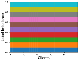
(a) IID splitting.

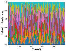
(b) Dir-1.0 splitting.

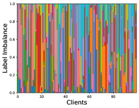
(c) Dir-0.1 splitting.

​​​​ ​​​​

Figure 4: Label ratios under different splitting manners. Different color means the samples are in different labels. We show the different splitting distributions on a total of 100 clients.

We use the CIFAR-10 / 100 datasets to validate the efficiency, which is widely used to verify the federated efficiency (McMahan et al., 2017; Karimireddy et al., 2020; Li et al., 2020; Xu et al., 2021; Durmus et al., 2021; Gong et al., 2022; Wang et al., 2022; Fan et al., 2022; Caldarola et al., 2022; Sun et al., 2023b, a; Li et al., 2023a; Fan et al., 2024a, b). The total dataset of both contain 50,000 training samples and 10,000 test samples of 10 / 100 classes. Each is a colorful image in the size of 32$\times$32. We follow the training as the vanilla SGD to add data augmentation without additional operations.

Label Heterogeneity. For the dataset splitting, we adopt the label imbalanced splitting under the Dirichlet manners. We first generate a distribution matrix and then generate a random number to sample each data. To further enhance the local heterogeneity, we also adopt the sampling with replacement, which means one data sample may exist on several clients simultaneously. This is more related to real-world scenarios because of the local unknown dataset distribution. We generate the matrices in Fig. 4 to show their distribution differences. We can clearly see that Dir-0.1 introduces a very large heterogeneity in that there is almost one dominant class in a client. Dir-1.0 handles approximately 3 classes in one client. Actually, in practical scenarios, label imbalance may be the most popular heterogeneity because we often expect both the local task and local dataset to be still unknown to others. For instance, client $i$ may be an expert on task $A$, and client $j$ may be an expert on another task $B$. To combine the tasks $A$ and $B$, if we can directly merge them with a training policy without beforehand knowing the tasks, then it must further enhance local privacy.

Brightness Heterogeneity. To further simulate the real-world manners, we allow different clients to change the brightness and ratios of different color channels. This corresponds to different sources of data collected by different local clients. We show some samples in Fig. 5 to show how different they are on different clients. Specifically, after splitting the local dataset, we will calculate the average brightness of each local dataset. Then we generate a noise from Gaussian to randomly change the brightness and one of the color channels, which means that even similar samples have large color differences on different clients.

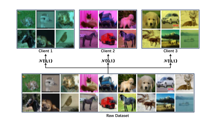
Figure 5: Introducing the brightness biases to different clients. We calculate the average brightness to control each sample to a proper state. Each client will randomly sample a Gaussian noise to perturb the local samples.

A.4 Additional Experiments

A.4.1 Some Training Curves

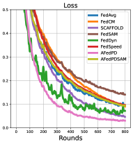
(a) Loss IID.

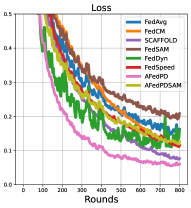
(b) Loss Dir-1.0.

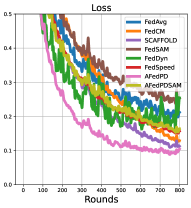
(c) Loss Dir-0.6.

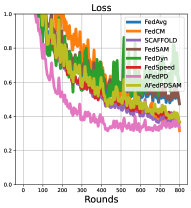
(d) Loss Dir-0.1.

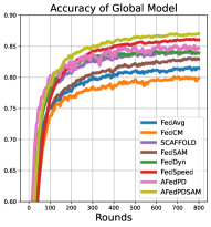
(e) Acc IID.

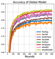
(f) Acc Dir-1.0.

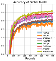
(g) Acc Dir-0.6.

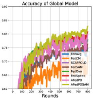
(h) Acc Dir-0.1.

Figure 6: Loss and accuracy curves in the experiments.

In Figure 6 we can see some experiment curves. From the (a), (b), (c), and (d), we can clearly see that the A-FedPD method achieves the fastest convergence rate on each setup. Due to the virtual update on the dual variables, we can treat those unparticipated clients as virtually trained ones. This empowers the A-FedPD method with a great convergence speed. Especially on the IID dataset, due to the local datasets being similar (drawn from a global distribution), the expectation of the updated averaged models is the same as that of the updated local model with lower variance. Then we could approximate the local dual update as the global one. This greatly speeds up the training time. We also can see the fast rate of the FedDyn method. However, due to its lagging dual update, it will be slower than the A-FedPD method. As for the SAM variant, it introduces an additional perturbation step that could avoid overfitting. Therefore, its loss does not drop quickly because of the additional ascent step.

From the (e), (f), (g), and (h), we can clearly see the improvements of A-FedPD and A-FedPDSAM methods. From the basic version, A-FedPD could achieve higher performance due to the virtual dual updates. After incorporating SAM, local clients could efficiently alleviate overfitting. The global model becomes more stable and could achieve the SOTA results. We will learn the consistency performance in the next part.

A.4.2 Primal Residual and Dual Residual

In the primal dual methods, due to the joint solution on both the primal and dual problems, it leads to an issue that both residuals should maintain a proper ratio. Therefore, the quantity of global updates in the training could be considered as a residual for the dual feasibility condition. The same, the constraint itself could be considered as the primal residual. Then we consider Eq.(3) objectives. The constraint is the global consensus level $\theta-\theta_{i}$ and the global update is $\theta^{t+1}-\theta^{t}$. To generally express them, we define the primal residual $p_{r}^{t}=\frac{1}{C}\sum_{i}\|\theta^{t}-\theta_{i}^{t}\|$ and the dual residual $d_{r}^{t}=\rho\|\theta^{t}-\theta^{t-1}\|$. Actually, the primal residual could be considered as the consistency, and the dual residual could be considered as the update. In the training, if we focus more on the dual residual, it leads to a fast convergence on an extremely biased objective that is far away from the true optimal. If we focus more on the primal residual, the local training cannot perform normally for its strong regularizations. Therefore, we must maintain stable trends on both $p_{r}$ and $d_{r}$ to implement stable training. In this part, we study the relationships between primal and dual residuals.

(a) Residuals on the CIFAR-10 test.

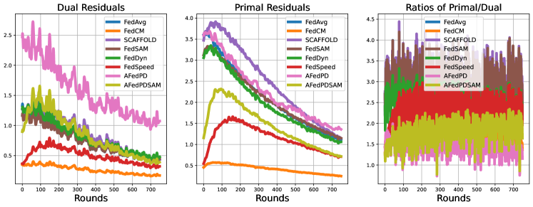
(b) Residuals on the CIFAR-100 test.

Figure 7: Loss and accuracy curves in the experiments.

As shown in Figure 7, we can clearly see the lower stable ratio between the primal and dual residuals on the A-FedPD and A-FedPDSAM methods, which indicates that both the primal training and dual training are performed well simultaneously. However, the federated primal average-based methods, i.e., FedAvg and SCAFFOLD, focus more on the primal training which leads to the dual residuals are too small (dual residuals measure the global update; primal residuals measure the global consistency).

A.4.3 Communication Efficiency

In this part, we learn the general communication efficiency. We fix all local intervals, clients, participation ratios, and hyperparameters for fairness. We select the different targets as the objective to calculate the communication efficiency.

Table 4: Communication rounds required to achieve the target accuracy.

CIFAR-10	FedAvg	SCAFFOLD	FedSAM	FedDyn	FedSpeed	A-FedPD	A-FedPDSAM
81%	501	207	345	156	170	131	156
	1$\times$	2.42$\times$	1.45$\times$	3.21$\times$	2.94$\times$	3.82$\times$	3.21$\times$
83.5%	-	468	-	355	268	252	218
	-	1$\times$	-	1.31$\times$	1.74$\times$	1.85$\times$	2.14$\times$
CIFAR-100	FedAvg	SCAFFOLD	FedSAM	FedDyn	FedSpeed	A-FedPD	A-FedPDSAM
40%	772	162	572	173	222	123	126
	1$\times$	4.76$\times$	1.34$\times$	4.46$\times$	3.47$\times$	6.27$\times$	6.12$\times$
49%	-	677	-	495	421	303	220
	-	1$\times$	-	1.36$\times$	1.61$\times$	2.23$\times$	3.07$\times$

Table 4 shows the communication efficiency among different methods on the CIFAR-10 / 100 dataset trained with LeNet. We calculate the first communication round index of achieving the target accuracy for comparison. We can clearly see that the communication rounds required for training are saved a lot on the proposed A-FedPD and A-FedPDSAM methods. It generally accelerates the training process by at least 3$\times$ on CIFAR-10 and 6$\times$ on CIFAR-100 than the vanilla FedAvg method. Compared with the other benchmarks, our proposed method performs stably and efficiently.

A.4.4 Wall clock Time for Training Costs

Then we further study the wall clock time required in the training. We provide the experimental setups as follows.

Platform: Pytorch 2.0.1   Cuda: 11.7   Hardware: NVIDIA GeForce RTX 2080 Ti

Table 5: Wall clock time required to train 1 round (100 iterations) on ResNet.

	FedAvg	SCAFFOLD	FedSAM	FedDyn	FedSpeed	A-FedPD	A-FedPDSAM
s / round	22.06	36.01	39.21	34.03	56.10	37.61	60.63
	1$\times$	1.63$\times$	1.77$\times$	1.54$\times$	2.54$\times$	1.70$\times$	2.74$\times$

Table 6: Wall clock time required to train 1 round (100 iterations) on LeNet.

	FedAvg	SCAFFOLD	FedSAM	FedDyn	FedSpeed	A-FedPD	A-FedPDSAM
s / round	9.82	11.42	12.53	11.76	13.61	11.71	13.90
	1$\times$	1.16$\times$	1.27$\times$	1.19$\times$	1.38$\times$	1.19$\times$	1.41$\times$

Actually, the LeNet is too small for the GPU and the training time does not achieve the capacity, which leads to the close time costs in Table 6. We recommend referring to the cost ratio on the ResNet (Table 5), which is much closer to the real algorithmic efficiency.

Appendix B Proofs.

In this part, we mainly show the proof details of the main theorems in this paper. We will reiterate the background details in Sec.B.1. Then we introduce the important lemmas used in the proof in Sec.B.3.1, and show the proof details of the main theorems in Sec.B.3.2.

B.1 Preliminaries

Here we reiterate the background details in the proofs. To understand the stability efficiency, we follow Hardt et al. (2016); Lei and Ying (2020); Zhou et al. (2021); Sun et al. (2023e) to adopt the uniform stability analysis in our analysis. Through refining the local subproblem of the solution of the Augmented Lagrangian objective, we provide the error term of the primal and dual terms and their corresponding complexity bound in FL.

Before introducing the important lemmas, we re-summarize the pipelines in the analysis. According to the federated setups, we assume a global server coordinates a set of local clients $\mathcal{C}\triangleq\left\{i\right\}_{i=1}^{C}$ to train one model. Each client has a private dataset $\mathcal{S}_{i}=\left\{\zeta_{ij}\right\}_{j=1}^{S}$. We assume that the global joint dataset is the union of $\{\mathcal{S}_{1}\cup\mathcal{S}_{2}\cup\cdots\cup\mathcal{S}_{C}\}$. To study its stability, we assume there is another global joint dataset that contains at most one different data sample from $\mathcal{C}$. Let the index of the different pair be $(i^{\star},j^{\star})$. We train two global models $\theta^{T}$ and $\hat{\theta}^{T}$ on these two global joint datasets respectively and gauge their gaps during the training process.

Then we rethink the local solution of the local augmented Lagrangian function. According to the basic algorithm, we have:

$$\mathcal{L}_{i}(\theta,\lambda_{i}^{t},\theta^{t})=f_{i}(\theta)+\langle\lambda_{i}^{t},\theta-\theta^{t}\rangle+\frac{\rho}{2}\|\theta-\theta^{t}\|^{2}.$$ (12)

To upper bound its stability without loss of generality, we consider adopting the general SGD optimizer to solve the sub-problem via total $K$ iterations with the local learning rate $\eta^{t}$:

$$\theta_{i,k+1}^{t}=\theta_{i,k}^{t}-\eta^{t}\nabla\mathcal{L}_{i}(\theta_{i,k}^{t},\lambda_{i}^{t},\theta^{t})=\theta_{i,k}^{t}-\eta^{t}\left[g_{i,k}^{t}+\lambda_{i}^{t}+\rho\left(\theta_{i,k}^{t}-\theta^{t}\right)\right],$$ (13)

where $k$ is the index of local iterations ($0\leq k\leq K$).

B.2 Optimization

B.2.1 Important Lemmas

In this part, we mainly introduce some important lemmas adopted in the optimization proofs.

Motivated by Durmus et al. (2021), we assume the local client solves the inexact solution of each local Lagrangian function, therefore we have $\nabla f_{i}(\theta_{i}^{t+1})+\lambda_{i}^{t}+\rho(\theta_{i}^{t+1}-\theta^{t})=e$, where $e$ can be considered as an error variable with $\|e\|^{2}\leq\epsilon$. This can characterize the different solutions of the local sub-problems. We always expect the error to achieve zero. Durmus et al. (2021) only assume that the local solution is exact and this may be not possible in practice.

Lemma 1 ((Durmus et al., 2021)).

The conditionally expected gaps between the current averaged local parameters and last averaged local parameters satisfy:

$$\mathbb{E}_{t}\|\overline{\theta}^{t+1}-\overline{\theta}^{t}\|^{2}\leq\frac{1}{C}\sum_{i\in\mathcal{C}}\mathbb{E}_{t}\|\theta_{i}^{t+1}-\overline{\theta}^{t}\|^{2}.$$

Proof..

According to the averaged randomly sampling, we have:

$$\mathbb{E}_{t}\|\overline{\theta}^{t+1}-\overline{\theta}^{t}\|^{2} =\mathbb{E}_{t}\|\frac{1}{P}\sum_{i\in\mathcal{P}^{t}}\theta_{i}^{t+1}-\overline{\theta}^{t}\|^{2}\leq\frac{1}{P}\mathbb{E}_{t}\sum_{i\in\mathcal{P}^{t}}\|\theta_{i}^{t+1}-\overline{\theta}^{t}\|^{2}$$

$$=\frac{1}{P}\mathbb{E}_{t}\sum_{i\in\mathcal{C}}\|\theta_{i}^{t+1}-\overline{\theta}^{t}\|^{2}\cdot\mathbb{I}_{i}\leq\frac{1}{C}\sum_{i\in\mathcal{C}}\mathbb{E}_{t}\|\theta_{i}^{t+1}-\overline{\theta}^{t}\|^{2}.$$

$\mathbb{I}_{i}$ is the indicator function as $\mathbb{I}_{i}=1$ if $i\in\mathcal{P}^{t}$ else 0.

Lemma 2.

Under Assumption 1 and let the local solution be an $\epsilon$-inexact solution, the conditionally expected averaged local updates satisfy:

$$\left(1-\frac{4L^{2}}{\rho^{2}}\right)\frac{1}{C}\sum_{i\in\mathcal{C}}\mathbb{E}_{t}\|\theta_{i}^{t+1}-\overline{\theta}^{t}\|^{2}\leq\frac{8L^{2}}{\rho^{2}}\frac{1}{C}\sum_{i\in\mathcal{C}}\mathbb{E}_{t}\|\theta_{i}^{t}-\overline{\theta}^{t}\|^{2}+\frac{4L^{2}}{\rho^{2}}\mathbb{E}_{t}\|\nabla f(\overline{\theta}^{t})\|^{2}+\frac{4\epsilon}{\rho^{2}}.$$ (14)

Proof..

First, we reconstruct the update of the dual variable. From the updated rules, we have $\overline{\lambda_{i}}^{t+1}-\overline{\lambda_{i}}^{t}=\rho(\overline{\theta}^{t+1}-\theta^{t})$. From the first order condition of $\nabla f_{i}(\theta_{i}^{t+1})+\lambda_{i}^{t}+\rho(\theta_{i}^{t+1}-\theta^{t})=e$. By expanding Lemma 11 in (Durmus et al., 2021), then we have:

$$\quad\ \frac{1}{C}\sum_{i\in\mathcal{C}}\mathbb{E}_{t}\|\theta_{i}^{t+1}-\overline{\theta}^{t}\|^{2}$$

$$=\frac{1}{C}\sum_{i\in\mathcal{C}}\mathbb{E}_{t}\|\theta_{i}^{t+1}-\theta^{t}+\frac{1}{\rho}\overline{\lambda}^{t}\|^{2}$$

$$\leq\frac{4L^{2}}{\rho^{2}}\frac{1}{C}\sum_{i\in\mathcal{C}}\left(\mathbb{E}_{t}\|\theta_{i}^{t+1}-\overline{\theta}^{t}\|^{2}+2\mathbb{E}_{t}\|\theta_{i}^{t}-\overline{\theta}^{t}\|^{2}+\mathbb{E}_{t}\|\nabla f(\overline{\theta}^{t})\|^{2}\right)+\frac{4\epsilon}{\rho^{2}}.$$

Therefore, we can reconstruct its relationship as:

$$\left(1-\frac{4L^{2}}{\rho^{2}}\right)\frac{1}{C}\sum_{i\in\mathcal{C}}\mathbb{E}_{t}\|\theta_{i}^{t+1}-\overline{\theta}^{t}\|^{2}\leq\frac{8L^{2}}{\rho^{2}}\frac{1}{C}\sum_{i\in\mathcal{C}}\mathbb{E}_{t}\|\theta_{i}^{t}-\overline{\theta}^{t}\|^{2}+\frac{4L^{2}}{\rho^{2}}\mathbb{E}_{t}\|\nabla f(\overline{\theta}^{t})\|^{2}+\frac{4\epsilon}{\rho^{2}}.$$

This completes the proofs.

Lemma 3.

Under Assumption 1, the conditionally expected averaged local consistency satisfies:

$$\frac{1}{C}\sum_{i\in\mathcal{C}}\mathbb{E}_{t}\|\theta_{i}^{t+1}-\overline{\theta}^{t+1}\|^{2}\leq\frac{4}{C}\sum_{i\in\mathcal{C}}\mathbb{E}_{t}\|\theta_{i}^{t+1}-\overline{\theta}^{t}\|^{2}.$$ (15)

Proof..

According to the update rules, we have:

$$\frac{1}{C}\sum_{i\in\mathcal{C}}\mathbb{E}_{t}\|\theta_{i}^{t+1}-\overline{\theta}^{t+1}\|^{2} =\frac{1}{C}\sum_{i\in\mathcal{C}}\mathbb{E}_{t}\|\theta_{i}^{t+1}-\overline{\theta}^{t}+\overline{\theta}^{t}-\overline{\theta}^{t+1}\|^{2}$$

$$\leq\frac{2}{C}\sum_{i\in\mathcal{C}}\mathbb{E}_{t}\|\theta_{i}^{t+1}-\overline{\theta}^{t}\|^{2}+2\mathbb{E}_{t}\|\overline{\theta}^{t}-\overline{\theta}^{t+1}\|^{2}$$

$$\leq\frac{2}{C}\sum_{i\in\mathcal{C}}\mathbb{E}_{t}\|\theta_{i}^{t+1}-\overline{\theta}^{t}\|^{2}+\frac{2}{C}\sum_{i\in\mathcal{C}}\mathbb{E}_{t}\|\theta_{i}^{t+1}-\overline{\theta}^{t}\|^{2}$$

$$\leq\frac{4}{C}\sum_{i\in\mathcal{C}}\mathbb{E}_{t}\|\theta_{i}^{t+1}-\overline{\theta}^{t}\|^{2}.$$

This completes the proofs.

B.2.2 Proofs

According to the smoothness, we take the conditional expectation on round $t$ and expand the global function as:

$$\quad\ \mathbb{E}_{t}\left[f(\overline{\theta}^{t+1})\right]-f(\overline{\theta}^{t})$$

$$\leq\frac{L}{2}\mathbb{E}_{t}\|\overline{\theta}^{t+1}-\overline{\theta}^{t}\|^{2}+\mathbb{E}_{t}\langle\nabla f(\overline{\theta}^{t}),\overline{\theta}^{t+1}-\overline{\theta}^{t}\rangle$$

$$=\frac{L}{2}\mathbb{E}_{t}\|\overline{\theta}^{t+1}-\overline{\theta}^{t}\|^{2}+\mathbb{E}_{t}\langle\nabla f(\overline{\theta}^{t}),\frac{1}{C}\sum_{i\in\mathcal{C}}\theta_{i}^{t+1}-\overline{\theta}^{t}\rangle$$

$$=\frac{L}{2}\mathbb{E}_{t}\|\overline{\theta}^{t+1}-\overline{\theta}^{t}\|^{2}+\mathbb{E}_{t}\langle\nabla f(\overline{\theta}^{t}),\frac{1}{C}\sum_{i\in\mathcal{C}}\left(\theta_{i}^{t+1}-\theta^{t}\right)+\theta^{t}-\overline{\theta}^{t}\rangle$$

$$=\frac{L}{2}\mathbb{E}_{t}\|\overline{\theta}^{t+1}-\overline{\theta}^{t}\|^{2}-\mathbb{E}_{t}\langle\nabla f(\overline{\theta}^{t}),\frac{1}{C}\sum_{i\in\mathcal{C}}\frac{1}{\rho}\left(\nabla f_{i}(\theta_{i}^{t+1})+\lambda_{i}^{t}-e\right)-\frac{1}{\rho}\overline{\lambda}^{t}\rangle$$

$$=\frac{L}{2}\mathbb{E}_{t}\|\overline{\theta}^{t+1}-\overline{\theta}^{t}\|^{2}-\mathbb{E}_{t}\langle\nabla f(\overline{\theta}^{t}),\frac{1}{C}\sum_{i\in\mathcal{C}}\frac{1}{\rho}\nabla f_{i}(\theta_{i}^{t+1})\rangle$$

$$\leq\frac{L}{2}\mathbb{E}_{t}\|\overline{\theta}^{t+1}-\overline{\theta}^{t}\|^{2}+\frac{1}{2\rho}\mathbb{E}_{t}\|\nabla f(\overline{\theta}^{t})-\frac{1}{C}\sum_{i\in\mathcal{C}}\nabla f_{i}(\theta_{i}^{t+1})\|^{2}-\frac{1}{2\rho}\mathbb{E}_{t}\|\nabla f(\overline{\theta}^{t})\|^{2}$$

$$\leq\frac{L}{2}\mathbb{E}_{t}\|\overline{\theta}^{t+1}-\overline{\theta}^{t}\|^{2}+\frac{1}{2\rho}\frac{1}{C}\sum_{i\in\mathcal{C}}\mathbb{E}_{t}\|\nabla f_{i}(\overline{\theta}^{t})-\nabla f_{i}(\theta_{i}^{t+1})\|^{2}-\frac{1}{2\rho}\mathbb{E}_{t}\|\nabla f(\overline{\theta}^{t})\|^{2}$$

$$\leq\frac{L}{2}\mathbb{E}_{t}\|\overline{\theta}^{t+1}-\overline{\theta}^{t}\|^{2}+\frac{L^{2}}{2\rho}\frac{1}{C}\sum_{i\in\mathcal{C}}\mathbb{E}_{t}\|\overline{\theta}^{t}-\theta_{i}^{t+1}\|^{2}-\frac{1}{2\rho}\mathbb{E}_{t}\|\nabla f(\overline{\theta}^{t})\|^{2}$$

$$\leq\frac{L}{2}\left(1+\frac{L}{\rho}\right)\frac{1}{C}\sum_{i\in\mathcal{C}}\mathbb{E}_{t}\|\overline{\theta}^{t}-\theta_{i}^{t+1}\|^{2}-\frac{1}{2\rho}\mathbb{E}_{t}\|\nabla f(\overline{\theta}^{t})\|^{2}.$$

To simplify the expression, we define $R_{t}=\frac{1}{C}\sum_{i\in\mathcal{C}}\mathbb{E}_{t}\|\theta_{i}^{t+1}-\overline{\theta}^{t}\|^{2}$, $J_{t}=\frac{1}{C}\sum_{i\in\mathcal{C}}\mathbb{E}_{t}\|\theta_{i}^{t}-\overline{\theta}^{t}\|^{2}$. Actually from Lemma 2 and 3, we can reconstruct the relationship as:

$$\begin{cases}\mathbb{E}_{t}\left[f(\overline{\theta}^{t+1})\right]&\leq f(\overline{\theta}^{t})+\frac{L}{2}\left(1+\frac{L}{\rho}\right)R_{t}-\frac{1}{2\rho}\mathbb{E}_{t}\|\nabla f(\overline{\theta}^{t})\|^{2},\\ \left(1-\frac{4L^{2}}{\rho^{2}}\right)R_{t}&\leq\frac{32L^{2}}{\rho^{2}}R_{t-1}+\frac{4L^{2}}{\rho^{2}}\mathbb{E}_{t}\|\nabla f(\overline{\theta}^{t})\|^{2}+\frac{4\epsilon}{\rho^{2}},\end{cases}$$

Let the second inequality be multiplied by $q$ and add it to the first, we have:

$$\quad\ \mathbb{E}_{t}\left[f(\overline{\theta}^{t+1})\right]+\left[q\left(1-\frac{4L^{2}}{\rho^{2}}\right)-\frac{L}{2}\left(1+\frac{L}{\rho}\right)\right]R_{t}$$

$$\leq f(\overline{\theta}^{t})+q\frac{32L^{2}}{\rho^{2}}R_{t-1}-\left(\frac{1}{2\rho}-\frac{4qL^{2}}{\rho^{2}}\right)\mathbb{E}_{t}\|\nabla f(\overline{\theta}^{t})\|^{2}+\frac{4q\epsilon}{\rho^{2}}.$$

Then we discuss the selection of $q$. First, let $\frac{1}{2\rho}-\frac{4qL^{2}}{\rho^{2}}>0$ be positive, which requires $q<\frac{\rho}{8L^{2}}$. Then we let the following relationship hold:

$$q\left(1-\frac{4L^{2}}{\rho^{2}}\right)-\frac{L}{2}\left(1+\frac{L}{\rho}\right)=q\frac{32L^{2}}{\rho^{2}},$$

Thus it requires $2q=\frac{L(\rho^{2}+\rho L)}{\rho^{2}-36L^{2}}<\frac{\rho}{4L^{2}}$. We can solve this to get the range of the coefficient $\rho$ as:

$$\rho^{2}-4L^{3}\rho-36L^{2}-4L^{4}>0.$$

Then $\rho>\mathcal{O}(L^{3})$ satisfies all the conditions above.

Therefore, let $q=\frac{\rho}{32L^{2}}$ and then $q\frac{32L^{2}}{\rho^{2}}=\frac{1}{\rho}$. By further relaxing the last coefficient we have:

$$\mathbb{E}_{t}\left[f(\overline{\theta}^{t+1})\right]+\frac{1}{\rho}R_{t} \leq f(\overline{\theta}^{t})+\frac{1}{\rho}R_{t-1}-\frac{1}{\rho}\mathbb{E}_{t}\|\nabla f(\overline{\theta}^{t})\|^{2}+\frac{\epsilon}{8L^{2}\rho}.$$

Taking the full expectation and accumulating the above inequality from $t=0$ to $T-1$, we have:

$$\frac{1}{T}\sum_{t=1}^{T}\mathbb{E}\|\nabla f(\overline{\theta}^{t})\|^{2} \leq\frac{f(\overline{\theta}^{1})-\mathbb{E}\left[f(\overline{\theta}^{T+1})\right]}{T}+\frac{R_{0}-R_{T}}{\rho T}+\frac{\epsilon}{8L^{2}\rho}$$

$$\leq\frac{\rho\left[f(\overline{\theta}^{1})-f^{\star}\right]+R_{0}}{T}+\frac{\epsilon}{8L^{2}\rho}.$$

In the last inequality, $f^{\star}$ is the optimum of the function $f$. For the $R_{-1}$ term, we have $R_{0}=\frac{1}{C}\sum_{i\in\mathcal{C}}\mathbb{E}_{t}\|\theta_{i}^{1}-\overline{\theta}^{0}\|^{2}=\frac{1}{C}\sum_{i\in\mathcal{C}}\mathbb{E}_{t}\|\theta_{i}^{1}-\theta^{0}\|^{2}$ for $\theta^{0}=\overline{\theta}^{0}$.

Discussions of the optimization errors.

We show some classical results of the generalization errors in the following Table 7. Zhang et al. (2021) provides a first optimization analysis for the federated primal-dual methods. However, it requires all clients to participate in the training in each round (do not support partial participation). Wang et al. (2022); Gong et al. (2022) proposes to adopt partial participation for the federated primal-dual method and adopt a stronger assumption on the local solution. It proves that even though each local solution is different, the total optimization error can be bounded by the average of the trajectory of each local client. However, the initial bias may be affected by the factor $C$ under some special learning rate. Durmus et al. (2021) further provides a variant to calculate the global dual variable. It provides a lower constant for the $D$ term, which is $\frac{C}{P}D$ (faster than $CD$ in FedADMM). Our proposed method A-FedPD updates the virtual dual variables, which could approximate the full-participation training under the partial participation case. Therefore, compared with the result in (Durmus et al., 2021), we further provide a faster constant for the term $D$ ($\frac{C}{P}\times$ faster than FedDyn on the first term when $\rho$ is selected properly). If the initialization bias $D$ dominates the optimization errors, i.e. training from scratch, A-FedPD can greatly improve the training efficiency.

Table 7: Optimization rate of federated smooth non-convex objectives.

	Assumption	Optimization	reduce dual-drift?
Zhang et al. (2021)	smoothness, $\epsilon$-inexact solution	$\mathcal{O}(\frac{D}{T}+\epsilon)$	$\times$
Hu et al. (2022)	smoothness, $\epsilon_{i,t}$-inexact solution	$\mathcal{O}(\frac{CD}{PT}+\frac{1}{CT}\sum_{i,t}\epsilon_{i,t})$	$\times$
Durmus et al. (2021)	smoothness, exact solution	$\mathcal{O}(\frac{CD}{PT}+\frac{R_{0}}{T})$	$\times$
our	smoothness, $\epsilon$-inexact solution	$\mathcal{O}(\frac{D}{T}+\frac{R_{0}}{T}+\epsilon)$	$\sqrt{}$

Our Improvements.

In (Zhang et al., 2021), it must rely on the full participation. In (Gong et al., 2022; Wang et al., 2022), the impact of the initial bias is $\frac{C}{P}$ times. In (Durmus et al., 2021), it must rely on the local exact solution, which is an extremely ideal condition. Our results can achieve the $\mathcal{O}(\frac{1}{T})$ rate under the general assumptions and support the partial participation case.

B.3 Generalization

B.3.1 Important Lemmas

In this part, we mainly introduce some important lemmas adopted in our proofs. Let $\hat{\cdot}$ be the corresponding variable trained on the dataset $\hat{\mathcal{C}}$, and then we can explore the gaps of corresponding terms. We first consider the stability definition.

Lemma 4 (Hardt et al. (2016)).

Under Assumption 1 and 2, the model $\theta^{T}$ and $\hat{\theta}^{T}$ are generated on the two different datasets $\mathcal{C}$ and $\hat{\mathcal{C}}$ with the same algorithm. We can track the difference between these two sequences. Before we first select the different sample pairs, the difference is always $0$. Therefore, we define an event $\zeta$ to measure whether $\theta^{T}=\hat{\theta}^{T}$ still holds at $\tau_{0}$-th round. Let $H=\sup_{\theta,\xi}f(\theta,\xi)<+\infty$, if the algorithm is uniform stable, we can measure its uniform stability by:

$$\epsilon_{G}\leq\sup_{\mathcal{C},\hat{\mathcal{C}},\xi}\mathbb{E}\left[f(\theta^{T},\xi)-f(\hat{\theta}^{T},\xi)\right]\leq G\mathbb{E}\|\theta^{T}-\hat{\theta}^{T}\|+\frac{HP\tau_{0}}{CS}.$$ (16)

Proof..

By expanding the inequality, we have:

$$\quad\ \mathbb{E}\left[|f(\theta^{T},\xi)-f(\hat{\theta}^{T},\xi)|\right]$$

$$\leq P(\zeta)\mathbb{E}\left[|f(\theta^{T},\xi)-f(\hat{\theta}^{T},\xi)|\ |\ \zeta\right]+P(\zeta^{c})\mathbb{E}\left[|f(\theta^{T},\xi)-f(\hat{\theta}^{T},\xi)|\ |\ \zeta^{c}\right]$$

$$\leq G\mathbb{E}\left[\|\theta^{T}-\hat{\theta}^{T}\|\ |\ \zeta\right]+HP(\zeta^{c}).$$

Here we assume that the difference pairs are selected on $\tau$-th round, therefore we have:

$$P(\zeta^{c}) =P(\tau\leq\tau_{0})\leq\sum_{t=0}^{\tau_{0}}P(\tau=t)=\sum_{t=0}^{\tau_{0}}P(i^{\star}\in\mathcal{P}^{t})P(j^{\star})\leq\frac{P\tau_{0}}{CS}.$$

This completes the proofs.

Specifically, because $\mathcal{C}$ only differs from $\hat{\mathcal{C}}$ on client $i^{\star}$, we could bound each term on two different situations respectively.

We consider the difference of the local updates on the client $i$ ($i\neq i^{\star}$).

Lemma 5.

Under Assumption 1, we can bound the difference of the local updates on the active client $i$ ($i\neq i^{\star}$). The local update satisfies:

$$\mathbb{E}\|\left(\theta_{i,k+1}^{t}-\theta^{t}\right)-\left(\hat{\theta}_{i,k+1}^{t}-\hat{\theta}^{t}\right)\|\leq\eta^{t}KL\mathbb{E}\|\theta^{t}-\hat{\theta}^{t}\|+\eta^{t}K\mathbb{E}\|\lambda_{i}^{t}-\hat{\lambda}_{i}^{t}\|.$$ (17)

Proof..

Reconstructing Eq.(13) we can get the following iteration relationship:

$$\theta_{i,k+1}^{t}-\theta^{t}=\left(1-\eta^{t}\rho\right)\left(\theta_{i,k}^{t}-\theta^{t}\right)-\eta^{t}\left(g_{i,k}^{t}+\lambda_{i}^{t}\right).$$

On each client $i$ ($i\neq i^{\star}$), each data sample is the same, thus we have:

$$\quad\ \mathbb{E}\|\left(\theta_{i,k+1}^{t}-\theta^{t}\right)-\left(\hat{\theta}_{i,k+1}^{t}-\hat{\theta}^{t}\right)\|$$

$$=\mathbb{E}\|\left(1-\eta^{t}\rho\right)\left[\left(\theta_{i,k}^{t}-\theta^{t}\right)-\left(\hat{\theta}_{i,k}^{t}-\hat{\theta}^{t}\right)\right]-\eta^{t}\left(g_{i,k}^{t}-\hat{g}_{i,k}^{t}\right)-\eta^{t}\left(\lambda_{i}^{t}-\hat{\lambda}_{i}^{t}\right)\|$$

$$\leq\left(1-\eta^{t}\rho\right)\mathbb{E}\|\left(\theta_{i,k}^{t}-\theta^{t}\right)-\left(\hat{\theta}_{i,k}^{t}-\hat{\theta}^{t}\right)\|+\eta^{t}L\mathbb{E}\|\theta_{i,k}^{t}-\hat{\theta}_{i,k}^{t}\|+\eta^{t}\mathbb{E}\|\lambda_{i}^{t}-\hat{\lambda}_{i}^{t}\|$$

$$\leq\left(1-\eta^{t}\rho_{L}\right)\mathbb{E}\|\left(\theta_{i,k}^{t}-\theta^{t}\right)-\left(\hat{\theta}_{i,k}^{t}-\hat{\theta}^{t}\right)\|+\eta^{t}L\mathbb{E}\|\theta^{t}-\hat{\theta}^{t}\|+\eta^{t}\mathbb{E}\|\lambda_{i}^{t}-\hat{\lambda}_{i}^{t}\|.$$

where $\rho_{L}=\rho-L$ is a constant.

Unrolling the recursion from $k=0$ to $K-1$, and adopting the factors $\theta_{i}^{t+1}=\theta_{i,k}^{t}$ and $\theta_{i,0}^{t}=\theta^{t}$, we have:

$$\quad\ \mathbb{E}\|\left(\theta_{i}^{t+1}-\theta^{t}\right)-\left(\hat{\theta}_{i}^{t+1}-\hat{\theta}^{t}\right)\|=\mathbb{E}\|\left(\theta_{i,k}^{t}-\theta^{t}\right)-\left(\hat{\theta}_{i,k}^{t}-\hat{\theta}^{t}\right)\|$$

$$\leq\left[\prod_{k=0}^{K-1}\left(1-\eta^{t}\rho_{L}\right)\right]\mathbb{E}\|\left(\theta_{i,0}^{t}-\theta^{t}\right)-\left(\hat{\theta}_{i,0}^{t}-\hat{\theta}^{t}\right)\|$$

$$\quad+\sum_{k=0}^{K-1}\eta^{t}\left[\prod_{j=k+1}^{K-1}\left(1-\eta^{t}\rho_{L}\right)\right]\left(L\mathbb{E}\|\theta^{t}-\hat{\theta}^{t}\|+\mathbb{E}\|\lambda_{i}^{t}-\hat{\lambda}_{i}^{t}\|\right)$$

$$=\sum_{k=0}^{K-1}\eta^{t}\left[\prod_{j=k+1}^{K-1}\left(1-\eta^{t}\rho_{L}\right)\right]\left(L\mathbb{E}\|\theta^{t}-\hat{\theta}^{t}\|+\mathbb{E}\|\lambda_{i}^{t}-\hat{\lambda}_{i}^{t}\|\right).$$

Simplifying the relationships, we have:

$$\mathbb{E}\|\left(\theta_{i}^{t+1}-\theta^{t}\right)-\left(\hat{\theta}_{i}^{t+1}-\hat{\theta}^{t}\right)\| =\frac{1-\left(1-\eta^{t}\rho_{L}\right)^{K}}{\rho_{L}}\left(L\mathbb{E}\|\theta^{T}-\hat{\theta}^{T}\|+\mathbb{E}\|\lambda_{i}^{t}-\hat{\lambda}_{i}^{t}\|\right)$$

$$\leq\eta^{t}KL\mathbb{E}\|\theta^{T}-\hat{\theta}^{T}\|+\eta^{t}K\mathbb{E}\|\lambda_{i}^{t}-\hat{\lambda}_{i}^{t}\|.$$

The last inequality adopts the Bernoulli inequality $\left(1+x\right)^{K}\geq 1+Kx$ for $K\geq 1$ and $x\geq-1$.

Then we consider the difference of the local updates on client $i^{\star}$.

Lemma 6.

Under Assumption 1 and 2, we can bound the difference of the local updates on the active client $i^{\star}$. The local update satisfies:

$$\mathbb{E}\|\left(\theta_{i,k+1}^{t}-\theta^{t}\right)-\left(\hat{\theta}_{i,k+1}^{t}-\hat{\theta}^{t}\right)\|\leq\eta^{t}KL\mathbb{E}\|\theta^{t}-\hat{\theta}^{t}\|+\eta^{t}K\mathbb{E}\|\lambda_{i}^{t}-\hat{\lambda}_{i}^{t}\|+\frac{2\eta^{t}KG}{s}.$$ (18)

Proof..

Reconstructing Eq.(13) we can get the following iteration relationship:

$$\theta_{i,k+1}^{t}-\theta^{t}=\left(1-\eta^{t}\rho\right)\left(\theta_{i,k}^{t}-\theta^{t}\right)-\eta^{t}\left(g_{i,k}^{t}+\lambda_{i}^{t}\right).$$

Lemma 5 shows the recursive formulation when we select the same data sample. However, on the client $i^{\star}$, it also may select the different sample pairs. Therefore, we first study the recursive formulation of this situation. When the stochastic gradients are calculated with different sample pairs $(\xi,\hat{\xi})$, we have:

$$\quad\ \mathbb{E}\|\left(\theta_{i,k+1}^{t}-\theta^{t}\right)-\left(\hat{\theta}_{i,k+1}^{t}-\hat{\theta}^{t}\right)\|$$

$$=\mathbb{E}\|\left(1-\eta^{t}\rho\right)\left[\left(\theta_{i,k}^{t}-\theta^{t}\right)-\left(\hat{\theta}_{i,k}^{t}-\hat{\theta}^{t}\right)\right]-\eta^{t}\left(g_{i,k}^{t}-\hat{g}_{i,k}^{t}\right)-\eta^{t}\left(\lambda_{i}^{t}-\hat{\lambda}_{i}^{t}\right)\|$$

$$\leq\left(1-\eta^{t}\rho\right)\mathbb{E}\|\left(\theta_{i,k}^{t}-\theta^{t}\right)-\left(\hat{\theta}_{i,k}^{t}-\hat{\theta}^{t}\right)\|+2\eta^{t}G+\eta^{t}\mathbb{E}\|\lambda_{i}^{t}-\hat{\lambda}_{i}^{t}\|.$$

For every single sample, the probability of selecting the $\xi_{j^{\star}}$ is $\frac{1}{S}$. Therefore, combining Lemma 5, we have:

$$\quad\ \mathbb{E}\|\left(\theta_{i,k+1}^{t}-\theta^{t}\right)-\left(\hat{\theta}_{i,k+1}^{t}-\hat{\theta}^{t}\right)\|$$

$$\leq\left(1-\frac{1}{S}\right)\left[\left(1-\eta^{t}\rho_{L}\right)\mathbb{E}\|\left(\theta_{i,k}^{t}-\theta^{t}\right)-\left(\hat{\theta}_{i,k}^{t}-\hat{\theta}^{t}\right)\|+\eta^{t}L\mathbb{E}\|\theta^{t}-\hat{\theta}^{t}\|+\eta^{t}\mathbb{E}\|\lambda_{i}^{t}-\hat{\lambda}_{i}^{t}\|\right]$$

$$\quad+\frac{1}{S}\left[\left(1-\eta^{t}\rho\right)\mathbb{E}\|\left(\theta_{i,k}^{t}-\theta^{t}\right)-\left(\hat{\theta}_{i,k}^{t}-\hat{\theta}^{t}\right)\|+2\eta^{t}G+\eta^{t}\mathbb{E}\|\lambda_{i}^{t}-\hat{\lambda}_{i}^{t}\|\right]$$

$$\leq\left(1-\eta^{t}\rho_{L}\right)\mathbb{E}\|\left(\theta_{i,k}^{t}-\theta^{t}\right)-\left(\hat{\theta}_{i,k}^{t}-\hat{\theta}^{t}\right)\|+\eta^{t}L\mathbb{E}\|\theta^{t}-\hat{\theta}^{t}\|+\eta^{t}\mathbb{E}\|\lambda_{i}^{t}-\hat{\lambda}_{i}^{t}\|+\frac{2\eta^{t}G}{s}.$$

Generally, we consider the size of samples $S$ to be large enough. In current deep learning, the dataset adopted usually maintains even millions of samples, which indicates that $1-\frac{1}{S}\rightarrow 1$.

Unrolling the recursion from $k=0$ to $K-1$ and adopting the $\theta_{i}^{t+1}=\theta_{i,K}^{t}$ and $\theta_{i,0}^{t}=\theta^{t}$, we have a similar relationship:

$$\quad\ \mathbb{E}\|\left(\theta_{i}^{t+1}-\theta^{t}\right)-\left(\hat{\theta}_{i}^{t+1}-\hat{\theta}^{t}\right)\|=\mathbb{E}\|\left(\theta_{i,k}^{t}-\theta^{t}\right)-\left(\hat{\theta}_{i,k}^{t}-\hat{\theta}^{t}\right)\|$$

$$\leq\sum_{k=0}^{K-1}\eta^{t}\left[\prod_{j=k+1}^{K-1}\left(1-\eta^{t}\rho_{L}\right)\right]\left(L\mathbb{E}\|\theta^{t}-\hat{\theta}^{t}\|+\mathbb{E}\|\lambda_{i}^{t}-\hat{\lambda}_{i}^{t}\|+\frac{2G}{s}\right).$$

Simplifying the relationships, we have:

$$\mathbb{E}\|\left(\theta_{i}^{t+1}-\theta^{t}\right)-\left(\hat{\theta}_{i}^{t+1}-\hat{\theta}^{t}\right)\| =\frac{1-\left(1-\eta^{t}\rho_{L}\right)^{K}}{\rho_{L}}\left(L\mathbb{E}\|\theta^{t}-\hat{\theta}^{t}\|+\mathbb{E}\|\lambda_{i}^{t}-\hat{\lambda}_{i}^{t}\|+\frac{2G}{s}\right)$$

$$\leq\eta^{t}KL\mathbb{E}\|\theta^{t}-\hat{\theta}^{t}\|+\eta^{t}K\mathbb{E}\|\lambda_{i}^{t}-\hat{\lambda}_{i}^{t}\|+\frac{2\eta^{t}KG}{s}.$$

The last inequality adopts the Bernoulli inequality.

B.3.2 Proofs

Table 8: Notations in the proofs.

Symbol	Formulation	Description
$\Delta^{t}$	$\mathbb{E}\|\theta^{t}-\hat{\theta}^{t}\|$	difference of the global parameters
$\delta^{t}$	$\frac{1}{C}\sum_{i\in\mathcal{C}}\mathbb{E}\|\theta_{i}^{t}-\hat{\theta}_{i}^{t}\|$	discrete difference of the local parameters
$\sigma^{t}$	$\frac{1}{C}\sum_{i\in\mathcal{C}}\mathbb{E}\|\lambda_{i}^{t}-\hat{\lambda}_{i}^{t}\|$	discrete difference of the dual variables
$\pi^{t}$	$\frac{1}{C}\sum_{i\in\mathcal{C}}\mathbb{E}\|(\theta_{i}^{t}-\theta^{t-1})-(\hat{\theta}_{i}^{t}-\hat{\theta}^{t-1})\|$	discrete difference of the local updates

In this part, we mainly introduce the proof of the main theorems. Combining the local updates and global updates, we can further upper bound both the primal and dual variables. Before proving the theorems, we first introduce the notations of updates of the global parameters and dual variables in Table 8.

$\Delta^{t}$ measures the difference of the primal models during the training. $\delta^{t}$ is the local separate difference when the local objective is solved. $\sigma^{t}$ measures the difference of the dual gaps. $\pi^{t}$ measures the difference of the local updates, which is also an important variable to connect global variables and dual variables. In our proofs, we first discuss the process of the primal variables and dual variables respectively. Then we can use the $\pi$ term to construct an inequality to eliminate redundant terms, which could further provide the recursive relationship of the primal variables and dual variables separately. Next, we introduce these three processes one by one.

From the global updates, according to the global aggregation and let $\mathbb{I}_{i}$ be the indicator function, we have:

$$\Delta^{t+1}=\mathbb{E}\|\theta^{t+1}-\hat{\theta}^{t+1}\| =\mathbb{E}\|\frac{1}{P}\sum_{i\in\mathcal{P}^{t}}\left(\theta_{i}^{t+1}-\hat{\theta}_{i}^{t+1}\right)+\frac{1}{\rho}\left(\overline{\lambda}_{i}^{t+1}-\hat{\overline{\lambda}}_{i}^{t+1}\right)\|$$

$$\leq\frac{1}{P}\mathbb{E}\sum_{i\in\mathcal{C}}\mathbb{E}\|\theta_{i}^{t+1}-\hat{\theta}_{i}^{t+1}\|\cdot\mathbb{I}_{i}+\frac{1}{\rho}\mathbb{E}\|\overline{\lambda}_{i}^{t+1}-\hat{\overline{\lambda}}_{i}^{t+1}\|$$

$$\leq\frac{1}{C}\sum_{i\in\mathcal{C}}\mathbb{E}\|\theta_{i}^{t+1}-\hat{\theta}_{i}^{t+1}\|+\frac{1}{C}\sum_{i\in\mathcal{C}}\frac{1}{\rho}\mathbb{E}\|\overline{\lambda}_{i}^{t+1}-\hat{\overline{\lambda}}_{i}^{t+1}\|\leq\delta^{t+1}+\frac{1}{\rho}\sigma^{t+1}.$$

From the dual updates, according to the local dual variable, we have two different cases. Combing the D-Update we have:

$$\overline{\lambda}^{t+1} =\frac{1}{C}\sum_{i\in\mathcal{C}}\lambda_{i}^{t+1}=\frac{1}{C}\sum_{i\in\mathcal{C}}\lambda_{i}^{t}+\frac{1}{C}\sum_{i\in\mathcal{P}^{t}}\rho(\theta_{i}^{t+1}-\theta^{t})+\frac{1}{C}\sum_{i\notin\mathcal{P}^{t}}\rho(\overline{\theta}^{t+1}-\theta^{t})$$

$$=\frac{1}{C}\sum_{i\in\mathcal{C}}\lambda_{i}^{t}+\frac{P}{C}\rho(\overline{\theta}^{t+1}-\theta^{t})+\frac{C-P}{C}\rho(\overline{\theta}^{t+1}-\theta^{t})=\overline{\lambda}^{t}+\rho(\overline{\theta}^{t+1}-\theta^{t}).$$

Considering the randomness of selecting $\mathcal{P}^{t}$ and expectation of $\overline{\theta}$, we have $\sigma^{t+1}\leq\sigma^{t}+\rho\pi^{t}$.

Here we add the additional definition of the unparticipated clients. We let the $\theta_{i}^{t+1}=\theta^{t}$ where $i\notin\mathcal{P}^{t}$, which enlarge the summation from $\mathcal{P}^{t}$ to $\mathcal{C}$. Then we summarize Lemma 5 and 6 as the following formulation:

$$\pi^{t+1} =\frac{1}{C}\sum_{i\in\mathcal{C}}\mathbb{E}\|\left(\theta_{i}^{t+1}-\theta^{t}\right)-\left(\hat{\theta}_{i}^{t+1}-\hat{\theta}^{t}\right)\|=\frac{1}{C}\sum_{i\in\mathcal{P}^{t}}\mathbb{E}\|\left(\theta_{i}^{t+1}-\theta^{t}\right)-\left(\hat{\theta}_{i}^{t+1}-\hat{\theta}^{t}\right)\|$$

$$<\eta^{t}KL\mathbb{E}\|\theta^{t}-\hat{\theta}^{t}\|+\eta^{t}K\frac{1}{C}\sum_{i\in\mathcal{C}}\mathbb{E}\|\lambda_{i}^{t}-\hat{\lambda}_{i}^{t}\|+\frac{2\eta^{t}KG}{CS}=c_{1}\Delta^{t}+c_{2}\sigma^{t}+c_{3}.$$

Finally, we can directly expand the $\pi$ term by the triangle inequality:

$$\delta^{t+1} =\frac{1}{C}\sum_{i\in\mathcal{C}}\mathbb{E}\|\theta_{i}^{t+1}-\hat{\theta}_{i}^{t+1}\|$$

$$\leq\frac{1}{C}\sum_{i\in\mathcal{C}}\mathbb{E}\|\left(\theta_{i}^{t+1}-\theta^{t}\right)-\left(\hat{\theta}_{i}^{t+1}-\hat{\theta}^{t}\right)\|+\frac{1}{C}\sum_{i\in\mathcal{C}}\mathbb{E}\|\theta^{t}-\hat{\theta}^{t}\|=\pi^{t+1}+\Delta^{t}.$$

Combing the above recursive formulations, we have:

$$\begin{cases}\Delta^{t+1}&\leq\delta^{t+1}+\frac{1}{\rho}\sigma^{t+1},\\ \sigma^{t+1}&\leq\sigma^{t}+\rho\pi^{t+1},\\ \delta^{t+1}&\leq\pi^{t+1}+\Delta^{t},\\ \pi^{t+1}&\leq c_{1}\Delta^{t}+c_{2}\sigma^{t}+c_{3}.\end{cases}$$

By multiplying three additional positive coefficients $\alpha$, $\beta$, and $\gamma$ on the last three inequalities respectively, and adding them to the first one, we have:

$$\Delta^{t+1}+\left(\alpha-\frac{1}{\rho}\right)\sigma^{t+1}+\left(\beta-1\right)\delta^{t+1}+\left(\gamma-\alpha\rho-\beta\right)\pi^{t+1} \leq\left(\beta+\gamma c_{1}\right)\Delta^{t}+\left(\alpha+\gamma c_{2}\right)\sigma^{t}+\gamma c_{3}.$$

By observing the LHS and RHS of the inequality, we notice that it could be summarized as a recursive formulation of $\Delta^{t}$ and $\sigma^{t}$ terms by selecting proper coefficients. Therefore, let the following conditions hold,

$$\beta-1 \geq 0,$$

$$\gamma-\alpha\rho-\beta \geq 0.$$

By simply selecting the minimal values of $\beta=1$ and $\gamma=1+\alpha\rho$, we have:

$$\Delta^{t+1}+\left(\alpha-\frac{1}{\rho}\right)\sigma^{t+1} =\Delta^{t+1}+\left(\alpha-\frac{1}{\rho}\right)\sigma^{t+1}+\left(\beta-1\right)\delta^{t+1}+\left(\gamma-\alpha\rho-\beta\right)\pi^{t+1}$$

$$\leq\left(\beta+\gamma c_{1}\right)\Delta^{t}+\left(\alpha+\gamma c_{2}\right)\sigma^{t}+\gamma c_{3}$$

$$\leq(1+\gamma\eta^{t}KL)\left(\Delta^{t}+\frac{\alpha+(1+\alpha\rho)\eta^{t}K}{1+(1+\alpha\rho)\eta^{t}KL}\right)+\frac{2\gamma\eta^{t}KG}{CS}.$$

Here we further let $\alpha-\frac{1}{\rho}\geq\frac{\alpha+(1+\alpha\rho)\eta^{t}K}{1+(1+\alpha\rho)\eta^{t}KL}$ to support the above recursive relationships. To satisfy this, we can solve the following inequality:

$$L(\alpha\rho)^{2}-\rho(\alpha\rho)-\left(L+\rho+\frac{1}{\eta^{t}K}\right)\geq 0.$$

From the fundamental knowledge of quadratic equations, we know that there must exist a positive number belonging to interval $\left[x^{+},+\infty\right]$ to satisfy the condition, where $x^{+}$ is the larger zero point of the equation $Lx^{2}-\rho x-\left(L+\rho+\frac{1}{\eta^{t}K}\right)=0$. We can solve $x^{+}=\frac{\rho+\sqrt{\rho^{2}+4L(L+\rho+\frac{1}{\eta^{t}K})}}{2L}=\frac{\rho+\sqrt{(\rho+2L)^{2}+\frac{4L}{\eta^{t}K}}}{2L}\leq 1+\frac{\rho}{L}+2\sqrt{\frac{L}{\eta^{t}K}}$. When we select the proper $\alpha\rho\geq x^{+}$, the above inequality always holds. This also indicates that $\alpha-\frac{1}{\rho}\geq\frac{x^{+}-1}{\rho}>\frac{1}{L}$. Here we denote $\alpha_{\rho}=\alpha-\frac{1}{\rho}$ and the previous definition $\gamma=1+\alpha\rho$ as two constant coefficients, we can simplify the final iteration relationship as:

$$\Delta^{t+1}+\alpha_{\rho}\sigma^{t+1} \leq\left(1+\gamma\eta^{t}KL\right)\left(\Delta^{t}+\alpha_{\rho}\sigma^{t}\right)+\frac{\gamma\eta^{t}KG}{CS}.$$

Unrolling this from $t=\tau_{0}$ to $T-1$ and adopting the factors of $\Delta^{\tau_{0}}=0$ and $\lambda^{\tau_{0}}=0$, we have:

(1) When the global learning rate is selected as a constant $\eta^{t}=\eta^{t}_{0}$ where the initial learning rate $\eta^{t}_{0}\leq\frac{1}{KL}$:

$$\Delta^{T}+\alpha_{\rho}\lambda^{T}\leq\sum_{t=\tau_{0}}^{T-1}\left(1+\gamma\eta^{t}_{0}KL\right)^{t}\frac{2\gamma\eta^{t}_{0}KG}{CS}<\frac{2G\left(1+\gamma\right)^{T}}{LCS}.$$

(2) When the global learning rate is selected as a decayed sequence $\eta^{t}=\frac{\eta_{0}}{t+1}$ where the initial learning rate $\eta_{0}\leq\frac{\mu}{\gamma K}$ where $\mu$ is a positive constant, we have:

$$\Delta^{T}+\alpha_{\rho}\lambda^{T} \leq\sum_{t=\tau_{0}}^{T-1}\left(\prod_{j=t}^{T-1}\left(1+\frac{\gamma\eta^{t}_{0}KL}{j+1}\right)\right)\frac{2\gamma\eta^{t}_{0}KG}{CS(t+1)}\leq\sum_{t=\tau_{0}}^{T-1}\exp\left(\gamma\eta^{t}_{0}KL\ln\left(\frac{T}{t+1}\right)\right)\frac{2\gamma\eta^{t}_{0}KG}{CS(t+1)}$$

$$=\frac{2\gamma\eta^{t}_{0}KGT^{\gamma\eta^{t}_{0}KL}}{CS}\sum_{t=\tau_{0}}^{T-1}\left(\frac{1}{t+1}\right)^{1+\gamma\eta^{t}_{0}KL}<\frac{2G}{LCS}\left(\frac{T}{\tau_{0}}\right)^{\mu L}.$$

Here we mainly focus on the case of the decayed learning rates. According to Lemma 4, we have:

$$\varepsilon_{G}\leq G\Delta^{T}+\frac{HP\tau_{0}}{CS}\leq\frac{2G^{2}}{LCS}\left(\frac{T}{\tau_{0}}\right)^{\mu L}+\frac{HP\tau_{0}}{CS}.$$

By selecting the proper $\tau_{0}=\left(\frac{2G^{2}}{HPL}\right)^{\frac{1}{1+\mu L}}T^{\frac{\mu L}{1+\mu L}}$, we can get the minimal error bound as:

$$\varepsilon_{G}\leq\frac{2}{CS}\left(\frac{2G^{2}}{L}\right)^{\frac{1}{1+\mu L}}\left(HPT\right)^{\frac{\mu L}{1+\mu L}}.$$

Discussions of the generalization errors.

We show some general results of the generalization errors in the following Table 9. We prove that the federated primal-dual family can benefit from the local interval $K$ than the vanilla SGD methods, which is one of the key properties of the primal-dual methods.

Table 9: Generalization error bounds of smooth non-convex objectives.

	Assumption	Generalization
Hardt et al. (2016)	Lipschitz	$\mathcal{O}(\frac{(KT)^{\frac{\mu L}{1+\mu L}}}{CS})$
Mohri et al. (2019)	Lipschitz, VC	$\mathcal{O}(\frac{TK}{\sqrt{CS}})$
Hu et al. (2022)	Lipschitz, Bernstein	$\mathcal{O}(\frac{TK}{\sqrt{CS}})$
Wu et al. (2023)	Lipschitz, Stochastic	$\mathcal{O}(\frac{\sqrt{T}}{C\sqrt{CS}})$
Sun et al. (2023d)	Lipschitz	$\mathcal{O}(\frac{(PKT)^{\frac{\mu L}{1+\mu L}}}{CS})$
our	Lipschitz	$\mathcal{O}(\frac{(PT)^{\frac{\mu L}{1+\mu L}}}{CS})$

References

- Asad et al. [2020] Muhammad Asad, Ahmed Moustafa, and Takayuki Ito. Fedopt: Towards communication efficiency and privacy preservation in federated learning. Applied Sciences, 10(8):2864, 2020.
- Boyd et al. [2011] Stephen Boyd, Neal Parikh, Eric Chu, Borja Peleato, Jonathan Eckstein, et al. Distributed optimization and statistical learning via the alternating direction method of multipliers. Foundations and Trends® in Machine learning, 3(1):1–122, 2011.
- Caldarola et al. [2022] Debora Caldarola, Barbara Caputo, and Marco Ciccone. Improving generalization in federated learning by seeking flat minima. In European Conference on Computer Vision, pages 654–672. Springer, 2022.
- Caldarola et al. [2023] Debora Caldarola, Barbara Caputo, and Marco Ciccone. Window-based model averaging improves generalization in heterogeneous federated learning. In Proceedings of the IEEE/CVF International Conference on Computer Vision, pages 2263–2271, 2023.
- Charles and Konečnỳ [2021] Zachary Charles and Jakub Konečnỳ. Convergence and accuracy trade-offs in federated learning and meta-learning. In International Conference on Artificial Intelligence and Statistics, pages 2575–2583. PMLR, 2021.
- Condat and Richtárik [2022] Laurent Condat and Peter Richtárik. Randprox: Primal-dual optimization algorithms with randomized proximal updates. arXiv preprint arXiv:2207.12891, 2022.
- Condat et al. [2023] Laurent Condat, Ivan Agarskỳ, Grigory Malinovsky, and Peter Richtárik. Tamuna: Doubly accelerated federated learning with local training, compression, and partial participation. arXiv preprint arXiv:2302.09832, 2023.
- Dieuleveut et al. [2021] Aymeric Dieuleveut, Gersende Fort, Eric Moulines, and Geneviève Robin. Federated-em with heterogeneity mitigation and variance reduction. Advances in Neural Information Processing Systems, 34:29553–29566, 2021.
- Durmus et al. [2021] Alp Emre Durmus, Zhao Yue, Matas Ramon, Mattina Matthew, Whatmough Paul, and Saligrama Venkatesh. Federated learning based on dynamic regularization. In International Conference on Learning Representations, 2021.
- Fan et al. [2022] Ziqing Fan, Yanfeng Wang, Jiangchao Yao, Lingjuan Lyu, Ya Zhang, and Qi Tian. Fedskip: Combatting statistical heterogeneity with federated skip aggregation. In 2022 IEEE International Conference on Data Mining (ICDM), pages 131–140. IEEE, 2022.
- Fan et al. [2023] Ziqing Fan, Jiangchao Yao, Ruipeng Zhang, Lingjuan Lyu, Yanfeng Wang, and Ya Zhang. Federated learning under partially disjoint data via manifold reshaping. Transactions on Machine Learning Research, 2023.
- Fan et al. [2024a] Ziqing Fan, Shengchao Hu, Jiangchao Yao, Gang Niu, Ya Zhang, Masashi Sugiyama, and Yanfeng Wang. Locally estimated global perturbations are better than local perturbations for federated sharpness-aware minimization. arXiv preprint arXiv:2405.18890, 2024a.
- Fan et al. [2024b] Ziqing Fan, Jiangchao Yao, Bo Han, Ya Zhang, Yanfeng Wang, et al. Federated learning with bilateral curation for partially class-disjoint data. Advances in Neural Information Processing Systems, 36, 2024b.
- Foret et al. [2020] Pierre Foret, Ariel Kleiner, Hossein Mobahi, and Behnam Neyshabur. Sharpness-aware minimization for efficiently improving generalization. arXiv preprint arXiv:2010.01412, 2020.
- Gong et al. [2022] Yonghai Gong, Yichuan Li, and Nikolaos M Freris. Fedadmm: A robust federated deep learning framework with adaptivity to system heterogeneity. In 2022 IEEE 38th International Conference on Data Engineering (ICDE), pages 2575–2587. IEEE, 2022.
- Grudzień et al. [2023a] Michał Grudzień, Grigory Malinovsky, and Peter Richtárik. Can 5th generation local training methods support client sampling? yes! In International Conference on Artificial Intelligence and Statistics, pages 1055–1092. PMLR, 2023a.
- Grudzień et al. [2023b] Michał Grudzień, Grigory Malinovsky, and Peter Richtárik. Improving accelerated federated learning with compression and importance sampling. arXiv preprint arXiv:2306.03240, 2023b.
- Hardt et al. [2016] Moritz Hardt, Ben Recht, and Yoram Singer. Train faster, generalize better: Stability of stochastic gradient descent. In International conference on machine learning, pages 1225–1234. PMLR, 2016.
- He et al. [2016] Kaiming He, Xiangyu Zhang, Shaoqing Ren, and Jian Sun. Deep residual learning for image recognition. In Proceedings of the IEEE conference on computer vision and pattern recognition, pages 770–778, 2016.
- Horváth et al. [2022] Samuel Horváth, Maziar Sanjabi, Lin Xiao, Peter Richtárik, and Michael Rabbat. Fedshuffle: Recipes for better use of local work in federated learning. arXiv preprint arXiv:2204.13169, 2022.
- Hsu et al. [2019] Tzu-Ming Harry Hsu, Hang Qi, and Matthew Brown. Measuring the effects of non-identical data distribution for federated visual classification. arXiv preprint arXiv:1909.06335, 2019.
- Hu et al. [2022] Xiaolin Hu, Shaojie Li, and Yong Liu. Generalization bounds for federated learning: Fast rates, unparticipating clients and unbounded losses. In The Eleventh International Conference on Learning Representations, 2022.
- Jhunjhunwala et al. [2022] Divyansh Jhunjhunwala, Pranay Sharma, Aushim Nagarkatti, and Gauri Joshi. Fedvarp: Tackling the variance due to partial client participation in federated learning. In Uncertainty in Artificial Intelligence, pages 906–916. PMLR, 2022.
- Kang et al. [2024] Heejoo Kang, Minsoo Kim, Bumsuk Lee, and Hongseok Kim. Fedand: Federated learning exploiting consensus admm by nulling drift. IEEE Transactions on Industrial Informatics, 2024.
- Karimireddy et al. [2020] Sai Praneeth Karimireddy, Satyen Kale, Mehryar Mohri, Sashank Reddi, Sebastian Stich, and Ananda Theertha Suresh. Scaffold: Stochastic controlled averaging for federated learning. In International conference on machine learning, pages 5132–5143. PMLR, 2020.
- Kim et al. [2022] Geeho Kim, Jinkyu Kim, and Bohyung Han. Communication-efficient federated learning with acceleration of global momentum. arXiv preprint arXiv:2201.03172, 2022.
- Krizhevsky et al. [2009] Alex Krizhevsky, Geoffrey Hinton, et al. Learning multiple layers of features from tiny images. 2009.
- LeCun et al. [1998] Yann LeCun, Léon Bottou, Yoshua Bengio, and Patrick Haffner. Gradient-based learning applied to document recognition. Proceedings of the IEEE, 86(11):2278–2324, 1998.
- Lei and Ying [2020] Yunwen Lei and Yiming Ying. Fine-grained analysis of stability and generalization for stochastic gradient descent. In International Conference on Machine Learning, pages 5809–5819. PMLR, 2020.
- Li et al. [2023a] Qinglun Li, Li Shen, Guanghao Li, Quanjun Yin, and Dacheng Tao. Dfedadmm: Dual constraints controlled model inconsistency for decentralized federated learning. arXiv preprint arXiv:2308.08290, 2023a.
- Li et al. [2020] Tian Li, Anit Kumar Sahu, Manzil Zaheer, Maziar Sanjabi, Ameet Talwalkar, and Virginia Smith. Federated optimization in heterogeneous networks. Proceedings of Machine learning and systems, 2:429–450, 2020.
- Li et al. [2023b] Yiwei Li, Chien-Wei Huang, Shuai Wang, Chong-Yung Chi, and Tony QS Quek. Privacy-preserving federated primal-dual learning for non-convex problems with non-smooth regularization. In 2023 IEEE 33rd International Workshop on Machine Learning for Signal Processing (MLSP), pages 1–6. IEEE, 2023b.
- Liu et al. [2023] Yixing Liu, Yan Sun, Zhengtao Ding, Li Shen, Bo Liu, and Dacheng Tao. Enhance local consistency in federated learning: A multi-step inertial momentum approach. arXiv preprint arXiv:2302.05726, 2023.
- Malinovskiy et al. [2020] Grigory Malinovskiy, Dmitry Kovalev, Elnur Gasanov, Laurent Condat, and Peter Richtarik. From local sgd to local fixed-point methods for federated learning. In International Conference on Machine Learning, pages 6692–6701. PMLR, 2020.
- McMahan et al. [2017] Brendan McMahan, Eider Moore, Daniel Ramage, Seth Hampson, and Blaise Aguera y Arcas. Communication-efficient learning of deep networks from decentralized data. In Artificial intelligence and statistics, pages 1273–1282. PMLR, 2017.
- Mishchenko et al. [2022] Konstantin Mishchenko, Grigory Malinovsky, Sebastian Stich, and Peter Richtárik. Proxskip: Yes! local gradient steps provably lead to communication acceleration! finally! In International Conference on Machine Learning, pages 15750–15769. PMLR, 2022.
- Mohri et al. [2019] Mehryar Mohri, Gary Sivek, and Ananda Theertha Suresh. Agnostic federated learning. In International Conference on Machine Learning, pages 4615–4625. PMLR, 2019.
- Niu and Wei [2023] Xiaochun Niu and Ermin Wei. Fedhybrid: A hybrid federated optimization method for heterogeneous clients. IEEE Transactions on Signal Processing, 71:150–163, 2023.
- Ozfatura et al. [2021] Emre Ozfatura, Kerem Ozfatura, and Deniz Gündüz. Fedadc: Accelerated federated learning with drift control. In 2021 IEEE International Symposium on Information Theory (ISIT), pages 467–472. IEEE, 2021.
- Pathak and Wainwright [2020] Reese Pathak and Martin J Wainwright. Fedsplit: An algorithmic framework for fast federated optimization. Advances in neural information processing systems, 33:7057–7066, 2020.
- Qu et al. [2022] Zhe Qu, Xingyu Li, Rui Duan, Yao Liu, Bo Tang, and Zhuo Lu. Generalized federated learning via sharpness aware minimization. In International Conference on Machine Learning, pages 18250–18280. PMLR, 2022.
- Remedios et al. [2020] Samuel W Remedios, John A Butman, Bennett A Landman, and Dzung L Pham. Federated gradient averaging for multi-site training with momentum-based optimizers. In Domain Adaptation and Representation Transfer, and Distributed and Collaborative Learning: Second MICCAI Workshop, DART 2020, and First MICCAI Workshop, DCL 2020, Held in Conjunction with MICCAI 2020, Lima, Peru, October 4–8, 2020, Proceedings 2, pages 170–180. Springer, 2020.
- Sarcheshmehpour et al. [2021] Yasmin Sarcheshmehpour, M Leinonen, and Alexander Jung. Federated learning from big data over networks. In ICASSP 2021-2021 IEEE International Conference on Acoustics, Speech and Signal Processing (ICASSP), pages 3055–3059. IEEE, 2021.
- Shen et al. [2021] Zebang Shen, Juan Cervino, Hamed Hassani, and Alejandro Ribeiro. An agnostic approach to federated learning with class imbalance. In International Conference on Learning Representations, 2021.
- Sun et al. [2023a] Yan Sun, Li Shen, Shixiang Chen, Liang Ding, and Dacheng Tao. Dynamic regularized sharpness aware minimization in federated learning: Approaching global consistency and smooth landscape. arXiv preprint arXiv:2305.11584, 2023a.
- Sun et al. [2023b] Yan Sun, Li Shen, Tiansheng Huang, Liang Ding, and Dacheng Tao. Fedspeed: Larger local interval, less communication round, and higher generalization accuracy. arXiv preprint arXiv:2302.10429, 2023b.
- Sun et al. [2023c] Yan Sun, Li Shen, Hao Sun, Liang Ding, and Dacheng Tao. Efficient federated learning via local adaptive amended optimizer with linear speedup. arXiv preprint arXiv:2308.00522, 2023c.
- Sun et al. [2023d] Yan Sun, Li Shen, and Dacheng Tao. Which mode is better for federated learning? centralized or decentralized. arXiv preprint arXiv:2310.03461, 2023d.
- Sun et al. [2023e] Yan Sun, Li Shen, and Dacheng Tao. Understanding how consistency works in federated learning via stage-wise relaxed initialization. arXiv preprint arXiv:2306.05706, 2023e.
- Tran Dinh et al. [2021] Quoc Tran Dinh, Nhan H Pham, Dzung Phan, and Lam Nguyen. Feddr–randomized douglas-rachford splitting algorithms for nonconvex federated composite optimization. Advances in Neural Information Processing Systems, 34:30326–30338, 2021.
- Tyou et al. [2023] Iifan Tyou, Tomoya Murata, Takumi Fukami, Yuki Takezawa, and Kenta Niwa. A localized primal-dual method for centralized/decentralized federated learning robust to data heterogeneity. IEEE Transactions on Signal and Information Processing over Networks, 2023.
- Wang et al. [2022] Han Wang, Siddartha Marella, and James Anderson. Fedadmm: A federated primal-dual algorithm allowing partial participation. In 2022 IEEE 61st Conference on Decision and Control (CDC), pages 287–294. IEEE, 2022.
- Wang et al. [2019] Jianyu Wang, Vinayak Tantia, Nicolas Ballas, and Michael Rabbat. Slowmo: Improving communication-efficient distributed sgd with slow momentum. arXiv preprint arXiv:1910.00643, 2019.
- Wang et al. [2020a] Jianyu Wang, Qinghua Liu, Hao Liang, Gauri Joshi, and H Vincent Poor. Tackling the objective inconsistency problem in heterogeneous federated optimization. Advances in neural information processing systems, 33:7611–7623, 2020a.
- Wang et al. [2020b] Jianyu Wang, Qinghua Liu, Hao Liang, Gauri Joshi, and H Vincent Poor. Tackling the objective inconsistency problem in heterogeneous federated optimization. Advances in neural information processing systems, 33:7611–7623, 2020b.
- Wang et al. [2023] Shuai Wang, Yanqing Xu, Zhiguo Wang, Tsung-Hui Chang, Tony QS Quek, and Defeng Sun. Beyond admm: a unified client-variance-reduced adaptive federated learning framework. In Proceedings of the AAAI Conference on Artificial Intelligence, volume 37, pages 10175–10183, 2023.
- Wu et al. [2023] Zheshun Wu, Zenglin Xu, Hongfang Yu, and Jie Liu. Information-theoretic generalization analysis for topology-aware heterogeneous federated edge learning over noisy channels. IEEE Signal Processing Letters, 2023.
- Xu et al. [2021] Jing Xu, Sen Wang, Liwei Wang, and Andrew Chi-Chih Yao. Fedcm: Federated learning with client-level momentum. arXiv preprint arXiv:2106.10874, 2021.
- Yuan et al. [2021] Honglin Yuan, Manzil Zaheer, and Sashank Reddi. Federated composite optimization. In International Conference on Machine Learning, pages 12253–12266. PMLR, 2021.
- Zhang et al. [2024] Ruipeng Zhang, Ziqing Fan, Jiangchao Yao, Ya Zhang, and Yanfeng Wang. Domain-inspired sharpness-aware minimization under domain shifts. arXiv preprint arXiv:2405.18861, 2024.
- Zhang and Hong [2021] Xinwei Zhang and Mingyi Hong. On the connection between fed-dyn and fedpd. FedDyn_FedPD. pdf, 2021.
- Zhang et al. [2021] Xinwei Zhang, Mingyi Hong, Sairaj Dhople, Wotao Yin, and Yang Liu. Fedpd: A federated learning framework with adaptivity to non-iid data. IEEE Transactions on Signal Processing, 69:6055–6070, 2021.
- Zhou et al. [2021] Pan Zhou, Hanshu Yan, Xiaotong Yuan, Jiashi Feng, and Shuicheng Yan. Towards understanding why lookahead generalizes better than sgd and beyond. Advances in Neural Information Processing Systems, 34:27290–27304, 2021.
- Zhou and Li [2023] Shenglong Zhou and Geoffrey Ye Li. Federated learning via inexact admm. IEEE Transactions on Pattern Analysis and Machine Intelligence, 2023.