“Oh LLM, I’m Asking Thee, Please Give Me a Decision Tree”: Zero-Shot Decision Tree Induction and Embedding with Large Language Models

Abstract

Large language models (LLMs) provide powerful means to leverage prior knowledge for predictive modeling when data is limited. In this work, we demonstrate how LLMs can use their compressed world knowledge to generate intrinsically interpretable machine learning models, i.e., decision trees, without any training data. We find that these zero-shot decision trees can surpass data-driven trees on some small-sized tabular datasets and that embeddings derived from these trees perform on par with data-driven tree-based embeddings on average. Our knowledge-driven decision tree induction and embedding approaches therefore serve as strong new baselines for data-driven machine learning methods in the low-data regime.

1 Introduction

Machine learning algorithms are data-hungry (Banko and Brill 2001; Halevy, Norvig, and Pereira 2009; Knauer and Rodner 2024), including intrinsically interpretable models like decision trees (Van Der Ploeg, Austin, and Steyerberg 2014). In many domains, though, large- or medium-sized datasets are not easily available. In the healthcare sector, for instance, data is often limited for diagnostic or prognostic modeling when medical conditions are rare or dropout rates at follow-up assessments are high, respectively (Moons et al. 2015, 2019; Steyerberg 2019). In such a low-data regime, training predictive models from scratch is challenging and it may be necessary to make extensive use of prior knowledge for valid and reliable inferences (Harrell 2015; Heinze, Wallisch, and Dunkler 2018; Knauer and Rodner 2023). In recent years, advances in natural language processing and computing have granted practitioners and researchers access to the condensed world knowledge from much of the web in the form of pretrained deep learning models, i.e., large language models (LLMs) (Anthropic 2024a; Google 2024b; OpenAI 2024b). Although LLMs provide powerful means to leverage prior knowledge for predictive modeling when data is scarce, interpreting their decisions remains an open challenge (Longo et al. 2024). Additionally, state-of-the-art LLMs are proprietary (Chiang et al. 2024) and therefore cannot be readily used with sensitive data (Anthropic 2024b; Google 2024a; OpenAI 2024a). This limits their applicability for domains where privacy is critical such as the clinical setting.

In this work, our contributions are as follows:

1. We show how state-of-the-art LLMs can be used for building intrinsically interpretable machine learning models, i.e., decision trees, without access to the model weights and without any training data (Sect. 3). The zero-shot setting naturally preserves the data privacy and thus broadens the applicability of LLMs for predictive modeling across industry verticals.

2. We demonstrate how our zero-shot decision trees can also serve as feature representations for downstream models (Sect. 4).

3. We offer a systematic comparison of our decision tree induction and embedding approaches with state-of-the-art machine learning methods on 13 public and 2 private tabular classification datasets in the low-data regime. We show that our knowledge-driven trees achieve a better performance than data-driven trees on 27% of the datasets and that our zero-shot representations are not statistically different from data-driven tree-based embeddings (Sect. 6). Therefore, we argue that our zero-shot induction and embedding approaches can serve as powerful new baselines that data-driven machine learning methods should surpass to show their efficacy.

2 Related Work

Listing 1 Prompt template for our zero-shot tree induction

⬇

[User]

I want you to induce a decision tree classifier based on features. I first give an example below. Then, I provide you with new features and want you to build a decision tree with a maximum depth of d using the most important features.

The tree should classify p.

Features:

sepal length (cm), sepal width (cm), petal length (cm), petal width (cm)

Decision tree:

|- petal width (cm) <= 0.80

| |- class: setosa

|- petal width (cm) > 0.80

| |- petal width (cm) <= 1.75

| | |- class: versicolor

| |- petal width (cm) > 1.75

| | |- class: virginica

Features:

f_1, ..., f_k

Decision tree:

Transferring knowledge from one task with more data to another task with less data, i.e., transfer learning, has a long history (Pan and Yang 2009). However, the compressed world knowledge within LLMs has opened up new dimensions to augment data-driven machine learning methods with prior knowledge. Embedding approaches extract feature representations from LLMs and apply them as inputs to downstream models (Peters et al. 2018). Fine-tuning approaches update the LLM parameters for downstream tasks (Howard and Ruder 2018). In-context learning, on the other hand, is an emergent ability in LLMs where training examples can be presented to LLMs via prompts, without any additional parameter training or updates (Brown et al. 2020). This does not only allow for rapid prototyping on new tasks (Hollmann et al. 2023; Sun et al. 2022), but also for easily incorporating additional knowledge by changing the prompt (Kojima et al. 2022; Wei et al. 2022). Although the exact working mechanism of in-context learning is not yet fully studied (Fu et al. 2024; Shen, Mishra, and Khashabi 2024; Xie et al. 2022), it has been shown that deep learning architectures that power modern LLMs, i.e., transformers and state space models, can in-context learn (sparse) linear functions, two-layer neural networks, and decision trees (Garg et al. 2022; Grazzi et al. 2024). With $\geq$ 1 training examples, decision rules or trees can thus not only be extracted from machine learning models using explainable artificial intelligence (XAI) approaches (Molnar 2022; Ribeiro, Singh, and Guestrin 2016, 2018), but also from LLMs using in-context learning (Li et al. 2023; Wang et al. 2024).

Most related to our work, Nam et al. (2024) recently leveraged LLMs to generate features for tabular data. First, they used an LLM to propose a new feature name and to find a rule for generating the new feature values using only a task description and the feature names, but without any training examples. Second, they augmented the data with the new feature, trained a decision tree on the new data, and obtained a validation score. Finally, they used the LLM to iteratively improve the feature generation rule given a task description and the feature names as well as previous rules, trained decision trees, and validation scores. However, the focus of our research is not on feature generation, which can be detrimental when data is scarce (Harrell 2015; Heinze, Wallisch, and Dunkler 2018; Knauer and Rodner 2023). Rather, we present the first approach to apply state-of-the-art LLMs for zero-shot model generation using in-context learning, i.e., we show how LLMs can build intrinsically interpretable trees without access to the model weights and without any training data (Sect. 3). Furthermore, we demonstrate how our zero-shot trees can also serve as effective feature representations, i.e., embeddings, for downstream models (Sect. 4).

3 Zero-Shot Decision Tree Induction

In the following, we present how state-of-the-art LLMs can be used to generate decision trees without any training data. We therefore go beyond prior research that has employed LLMs to generate new features for machine learning models (Nam et al. 2024). Our approach does not only allow us to leverage the prior knowledge within LLMs for predictive modeling, but also to extract interpretable decision rules from LLMs and to naturally respect the data privacy. This broadens the applicability of LLMs for domains where data is frequently scarce, interpretability is desirable, or data protection is mandatory, such as in the healthcare sector (Longo et al. 2024; Moons et al. 2015, 2019; Steyerberg 2019).

Listing 1 shows our prompting template for building a zero-shot decision tree $T$. We start each prompt by presenting some background context, followed by the actual task description. The prediction target $p\in\mathcal{P}$ and the tree’s maximum depth $d\in\mathbb{N}^{+}$ need to be set depending on the task. Most importantly, we employ in-context learning to provide the LLM with an output indicator, i.e., we encourage the LLM to output the decision tree in a textual format. Finally, we pass the $k\in\mathbb{N}^{+}$ feature names $f=[f_{1},...,f_{k}]\in\mathcal{F}$ to the LLM including, if applicable, the categorical values or measurement units in brackets. Since state-of-the-art LLMs have seen massive text corpora and datasets from the web during pretraining (Bordt, Nori, and Caruana 2024; Bordt et al. 2024), they can leverage their condensed world knowledge to transform feature names into decision trees, given that the feature names are meaningful (Appendix A). This allows the LLM to derive a mapping $\phi(p,f_{1},...,f_{k},d)\mapsto T$.

4 Zero-Shot Decision Tree Embedding

Zero-shot decision trees encode rich structural dependencies between the input features and prediction target. In this section, we show how our knowledge-driven trees can be used as feature representations, i.e., embeddings, for downstream models. While prior work has focused on generating tree-based embeddings in a data-driven way (Borisov et al. 2023; Moosmann, Triggs, and Jurie 2006), our approach allows us to extract task-specific embeddings from a pretrained LLM and augment data-driven machine learning models with the LLM’s compressed knowledge about the world.

Knowledge Distillation

Decision tree ensembles often achieve state-of-the results on tabular data (McElfresh et al. 2024), so we distill the knowledge from an LLM into $\geq$ 1 zero-shot decision trees for our embedding approach. Since employing similar trees within a single representation would not add much information, we leverage the LLM’s inherent stochasticity (set by the temperature) and further increase its degrees of freedom by letting it determine the maximum tree depths on its own. Our mapping $\phi$ becomes a sampling from a probability distribution $T\sim\phi(p,f_{1},...,f_{k})$. The sampling is followed by a transformation to an embedding that can be easily processed by downstream models.

Figure 1: Embedding transformation $\chi_{2}$ using the iris data decision tree from Listing 1 and a sample with a petal width of $1.70$. The 2 inner nodes of the structured tree $T$ are mapped to a binary embedding vector of dimension 2. Thus, information from the leaf nodes is indirectly embedded.

Embedding Transformation

Let $\mathcal{T}_{n}$ represent the set of decision trees with $n$ inner nodes and $\mathbb{X}$ the feature space. Then the mapping $\chi_{n}$ of the truth values of the inner nodes to a binary vector of length $n$ can be expressed as $\chi_{n}:\mathcal{T}_{n}\times\mathbb{X}\to\{0,1\}^{n}$. The entries of the resulting binary vector are $1$ if the condition of the corresponding inner node is satisfied for a sample $x\in\mathbb{X}$, and $0$ otherwise (Borisov et al. 2023). Figure 1 shows this mapping for the iris data decision tree from Listing 1 and a sample with a petal width of $1.70$. To embed a decision forest $(T_{1},\ldots,T_{m})\in\mathcal{T}_{n_{1}}\times...\times\mathcal{T}_{n_{m}}$ consisting of $m$ decision trees with $n_{1},\ldots,n_{m}$ inner nodes, we define the mapping $\chi$ as follows:

$$\chi:\mathcal{T}_{n_{1}}\times\ldots\times\mathcal{T}_{n_{m}}\times\mathbb{X}\to\{0,1\}^{n_{1}+\cdots+n_{m}}.$$

This mapping concatenates the individual binary vectors $\chi_{n_{1}}(T_{1},x),\ldots,\chi_{n_{m}}(T_{m},x)$ obtained from each zero-shot tree to form our final task-specific embedding for a sample $x\in\mathbb{X}$. We investigate a second embedding approach, which combines decision tree embeddings with the original data, in Appendix C.

In the next section, we thoroughly evaluate our zero-shot decision tree induction and embedding approaches against state-of-the-art machine learning methods.

5 Experimental Setup

	Ours			Interpretable models		AutoML and deep learning
Dataset	Claude 3.5 Sonnet	Gemini 1.5 Pro	GPT-4o	BSS	OCTs	Auto-Gluon	Auto-Prognosis	TabPFN
public median	0.70	0.54	0.58	0.84	0.87	0.89	0.91	0.91
bankruptcy	0.58	0.53	0.74	0.89	0.84	0.90	0.91	0.91
boxing1	0.79	0.40	0.54	0.70	0.79	0.82	0.75	0.80
boxing2	0.62	0.46	0.40	0.75	0.79	0.72	0.79	0.65
creditscore	0.67	0.68	0.21	0.89	1.00	0.98	1.00	0.96
japansolvent	0.75	0.29	0.29	0.82	0.73	0.86	0.78	0.91
colic	0.59	0.28	0.70	0.85	0.88	0.87	0.86	0.87
heart_h	0.78	0.10	0.29	0.87	0.84	0.86	0.84	0.86
hepatitis	0.90	0.88	0.23	0.87	0.88	0.88	0.81	0.90
house_votes_84	0.16	0.12	0.21	0.92	0.93	0.94	0.94	0.94
irish	0.69	0.65	0.64	0.69	1.00	1.00	1.00	1.00
labor	0.55	0.80	0.75	0.84	0.80	0.85	0.92	0.89
penguins	0.92	0.60	0.85	*	0.98	0.99	0.99	0.99
vote	0.56	0.59	0.56	0.11	0.74	0.94	0.94	0.95
private median	0.69	0.49	0.71	0.63	0.72	0.67	0.61	0.66
ACL injury	0.44	0.00	0.63	0.40	0.46	0.46	0.25	0.40
post-trauma	0.86	0.55	0.76	0.86	0.90	0.88	0.82	0.94

Table 1: Median test F1-score at 67%/33% train/test splits for our LLM-based zero-shot decision tree induction approach compared to the machine learning baselines. The best score among the zero-shot methods is highlighted. *BSS via Interpretable AI 3.1.1 does not support multiclass classifications.

In the following, we provide details on the experimental setup to assess our zero-shot decision tree induction (Sect. 3) and embedding (Sect. 4), including the datasets, preprocessing, machine learning baselines, and performance metrics.

Datasets

To evaluate our induction and embedding methods, we selected 13 small-sized tabular classification datasets from the public Penn Machine Learning Benchmarks (PMLB). Please refer to Appendix A for more details about the selection criteria and to Appendix B for more details about the PMLB datasets, including tests evaluating whether state-of-the-art LLMs know or have memorized these public datasets (Bordt, Nori, and Caruana 2024; Bordt et al. 2024). Overall, we found evidence of knowledge (54%) or partial memorization (62%) of the public datasets by at least 1 state-of-the-art LLM. Our performance estimates on these datasets may therefore be overoptimistic. To obtain unbiased performance estimates, we also included 2 small-sized tabular datasets that are private. The private datasets are not publicly available and hence cannot have been seen during the LLMs’ pretraining. The prediction target for these datasets was to classify whether the prognosis after musculoskeletal trauma or anterior cruciate ligament (ACL) injury was good or bad. Additional details can be found in Appendix B.

Decision Tree Induction Setup

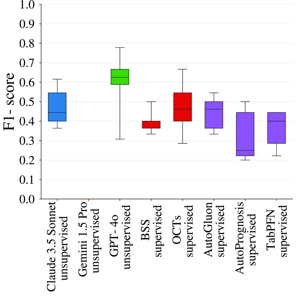
(a) F1-score on ACL injury data.

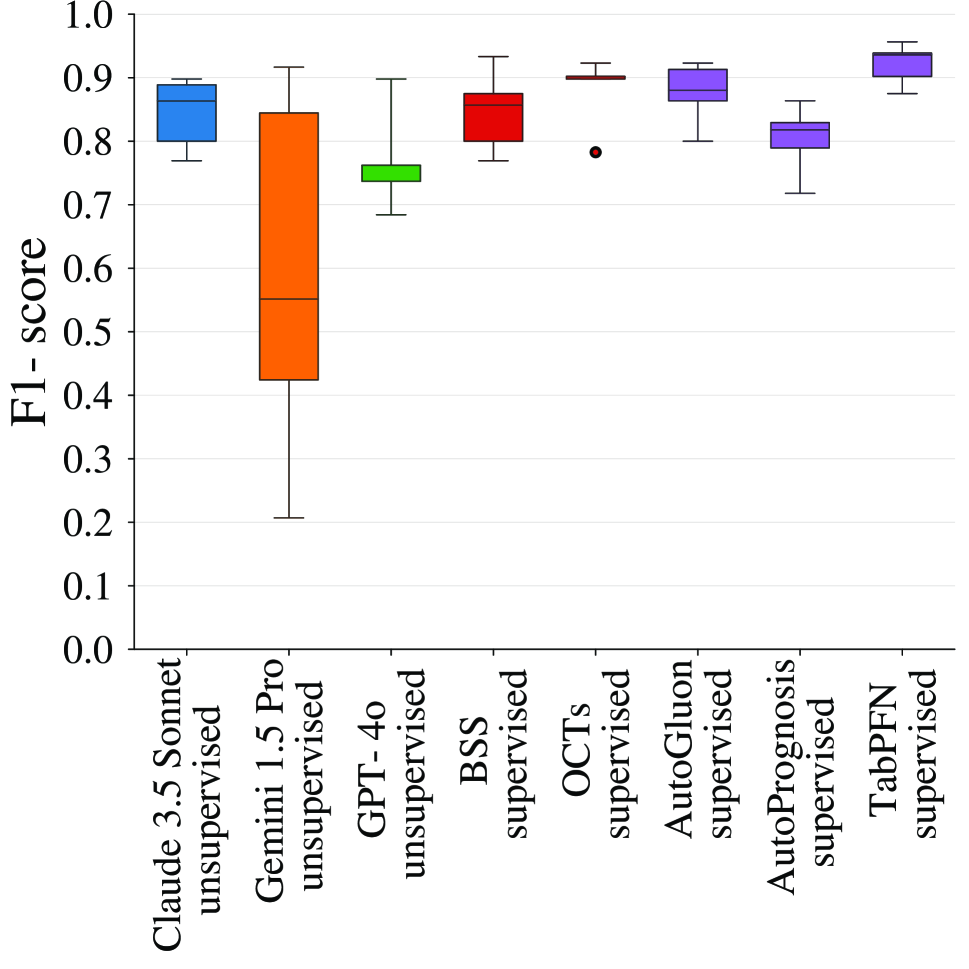
(b) F1-score on post-trauma pain data.

Figure 2: Test F1-score at 67%/33% train/test splits for our LLM-based zero-shot decision tree induction approach compared to the machine learning baselines on our private (a) ACL injury data and (b) post-trauma pain data. Note that the score for Gemini 1.5 Pro is 0 on the ACL injury data.

Methods

For our decision tree induction experiments, we used 3 state-of-the-art LLMs as well as 5 machine learning baselines, i.e., 2 data-driven intrinsically interpretable predictive models, 2 automated machine learning (AutoML) frameworks, and 1 off-the-shelf pretrained deep neural network.

Our zero-shot decision trees were generated with the top 3 LLMs on the LMSYS Chatbot Arena Leaderboard from July 1st, 2024 (Chiang et al. 2024): GPT-4o-2024-05-13 (OpenAI 2024b), Claude 3.5 Sonnet (Anthropic 2024a), and Gemini-1.5-Pro-API-0514 (Google 2024b). For all LLMs, we set the temperature to 0 for more determinstic outputs and fixed the maximum depth $d$ to 2 for more interpretable trees. However, we did not observe significant performance differences for other values of these hyperparameters in a smaller pre-evaluation. Furthermore, missing values were imputed using an optimal 10-nearest-neighbors-based imputation (Bertsimas, Pawlowski, and Zhuo 2018) before feeding test data to our trees.

As data-driven interpretable baselines, we applied cardinality-constrained best subset selection for logistic regression (BSS) (Bertsimas, Pauphilet, and Van Parys 2021) and optimal classification trees (OCTs) (Bertsimas and Dunn 2017) using Interpretable AI 3.1.1 with Gurobi 11.0.1. For preprocessing, we again imputed missing values. We then passed nominal feature indicators to both methods and used a 3-fold cross-validation with an F1-score validation criterion to find the best hyperparameters for BSS (i.e., the cardinality from the grid [1, 2, 3, 4] (Evans et al. 2022) and the regularization strength from the grid [0.1, 0.02, 0.004] (Knauer and Rodner 2023)). The maximum depth for the OCTs was chosen from the grid [1, 2]).

To obtain an upper bound on the predictive performance, we additionally evaluated 2 AutoML frameworks and 1 off-the-shelf pretrained deep neural network: AutoGluon 1.1.1 (Erickson et al. 2020; Salinas and Erickson 2024), AutoPrognosis 0.1.21 (Alaa and Schaar 2018; Imrie et al. 2023), and TabPFN 0.1.10 (Hollmann et al. 2023). AutoGluon, AutoPrognosis, and TabPFN have recently been shown to achieve a better mean rank in terms of discriminative performance than a simple logistic regression baseline in the low-data regime (Knauer and Rodner 2024). We used 32 ensemble members and one-hot encoded nominal features for TabPFN (Hollmann et al. 2023), selected the “best quality” preset for AutoGluon, passed nominal feature indicators to TabPFN and AutoGluon, and optimized AutoGluon and AutoPrognosis with an F1-score validation criterion. The runtime limit was 1h on an internal cluster (Rocky Linux 8.6) with 8 vCPU cores and 32 GiB memory (AMD Epyc 7352).

Evaluation Metrics

Our primary performance metrics were the test F1-score, i.e., the harmonic mean of precision and sensitivity (or recall), and the test balanced accuracy at a 67%/33% train/test split. For binary prediction targets, the balanced accuracy is equal to the arithmetic mean of specificity and sensitivity, or the area under the receiver operating characteristic curve with binary predictions rather than scores. The F1-score and the balanced accuracy are suitable for both binary and multiclass problems as well as balanced and imbalanced data (He and Ma 2013). Additionally, we evaluated the test F1-score and the test balanced accuracy at 50%/50% and 33%/67% train/test splits to assess the effect of reducing the training set size for our data-driven baselines. Each split was repeated 5 times to account for randomness in the split, the preprocessing, and the methods themselves. As there is no guarantee that syntactically correct zero-shot trees are generated, we performed API calls until 5 valid trees were found or a maximum number of iterations was reached (100 per LLM and dataset in our case).

Decision Tree Embedding Setup

		Ours			Unsupervised	Self-supervised			Supervised
Dataset	No embedding	Claude 3.5 Sonnet	Gemini 1.5 Pro	GPT-4o	Ran-dom trees	Extra trees	Ran-dom forest	XG-Boost	Extra trees	Ran-dom forest	XG-Boost
public median	0.78	0.00	-0.01	+0.02	-0.07	-0.14	-0.24	-0.02	-0.03	+0.01	+0.01
bankruptcy	0.94	-0.06	-0.18	-0.06	-0.18	-0.12	-0.06	-0.12	-0.12	-0.12	-0.06
boxing1	0.64	+0.02	-0.06	+0.06	+0.04	-0.11	-0.10	+0.08	-0.04	-0.07	+0.08
boxing2	0.61	+0.16	+0.13	+0.15	+0.04	+0.04	-0.09	+0.01	0.00	+0.09	+0.06
creditscore	0.75	-0.13	-0.13	-0.11	-0.13	+0.21	+0.18	-0.26	-0.06	+0.21	+0.21
japansolvent	0.83	0.00	-0.06	-0.12	-0.12	-0.35	-0.35	-0.11	0.00	0.00	-0.06
colic	0.80	-0.28	-0.01	+0.01	-0.12	-0.35	-0.41	-0.03	-0.06	-0.01	+0.01
heart_h	0.78	+0.01	-0.01	+0.01	-0.06	-0.33	-0.39	+0.03	-0.01	+0.01	-0.02
hepatitis	0.73	-0.05	-0.09	+0.02	-0.06	-0.29	-0.30	-0.09	-0.03	-0.15	-0.04
house_votes_84	0.96	-0.01	-0.02	0.00	-0.02	-0.06	-0.06	0.00	-0.01	-0.02	-0.01
irish	0.77	+0.01	+0.21	+0.18	+0.18	-0.08	-0.10	+0.18	+0.07	+0.14	+0.23
labor	0.94	-0.22	-0.21	-0.13	-0.12	-0.23	-0.22	-0.05	-0.19	-0.15	-0.19
penguins	1.00	0.00	0.00	0.00	-0.04	-0.35	-0.44	-0.37	-0.11	-0.08	-0.02
vote	0.50	+0.29	+0.28	+0.33	+0.13	-0.07	-0.03	+0.30	+0.12	+0.29	+0.30
private median	0.50	+0.04	+0.05	+0.09	+0.01	+0.05	-0.04	+0.11	+0.05	+0.09	+0.02
ACL injury	0.38	+0.12	0.00	+0.20	+0.11	+0.28	+0.11	+0.12	+0.18	+0.20	+0.06
post-trauma	0.62	-0.03	+0.10	-0.02	-0.08	-0.18	-0.18	+0.10	-0.08	-0.02	-0.02

Table 2: Median test F1-score at 67%/33% train/test splits of a linear model without embeddings (first column). Subsequent columns display the performance difference of our LLM-based zero-shot decision tree embedding approach as well as the unsupervised, self-supervised, and supervised embedding baselines relative to the first column. If there is an improvement compared to no embedding, the best score among the unsupervised methods is highlighted.

Methods

For our decision tree embedding experiments, we used the same 3 state-of-the-art LLMs as in our induction setup. To introduce greater variability in our tree generation, though, we set the LLMs’ temperature to their respective default values (0.7 for GPT-4o, 1.0 for Claude 3.5 Sonnet, and 1.0 for Gemini 1.5 Pro), fostering more diverse and creative outputs (Sect. 4). We then generated 5 decision trees for each LLM to form our decision forest for the embedding. The embeddings were used as feature representations for a simple linear probe, i.e., a logistic regression classifier.

Our zero-shot embeddings are inherently unsupervised, so our primary competitor was an unsupervised random trees embedding (Moosmann, Triggs, and Jurie 2006). We also fitted random forests (Breiman 2001), extremely randomized trees (Geurts, Ernst, and Wehenkel 2006), and XGBoost (Chen and Guestrin 2016) with 5 trees on our design matrices or labels to derive self-supervised or supervised tree embeddings (Borisov et al. 2023). A logistic regression classifier without any embedding served as a baseline for our experiments. The random trees embedding, random forest, extremely randomized trees, and logistic regression were run from scikit-learn 1.5.1, XGBoost from the XGBoost Python package 2.1.0. For all methods, missing values were imputed and nominal features one-hot encoded.

Evaluation Metrics

We assessed the predictive performance of each method with the test F1-score and balanced accuracy at a $33\%/67\%$ train/test split. We again repeated the split 5 times to account for randomness. To gain a deeper understanding of our LLM-based embedding approach, we evaluated the dimensionality of our embeddings (an indirect measure of the maximum tree depths chosen by the LLMs) and the selected feature variability (an indirect measure of the LLMs’ output diversity) per LLM and dataset, the effect of changing the decision forest size (as a plausibility check for our default forest size of 5), as well as the effect of concatenating our embeddings to the original feature vectors.

6 Experimental Results

In this section, we present the experimental results for our zero-shot decision tree induction (Sect. 3) and embedding (Sect. 4). Overall, we found that Claude 3.5 Sonnet yielded deterministic responses (except once) and that Gemini 1.5 Pro frequently needed multiple API calls to derive our zero-shot trees. Furthermore, we noted that the LLMs often generated explanations in addition to the decision trees, which can provide valuable insights into their reasoning processes. In terms of predictive performance, we found that LLM-based zero-shot decision tree generations showed a better average overall performance than the data-driven OCTs on 27% of our evaluated datasets, and that our zero-shot decision tree embeddings were not statistically different from the best data-driven tree-based embeddings. We therefore argue that our knowledge-driven induction and embedding approaches serve as powerful baselines for data-driven machine learning methods in the low-data regime.

Decision Tree Induction Results

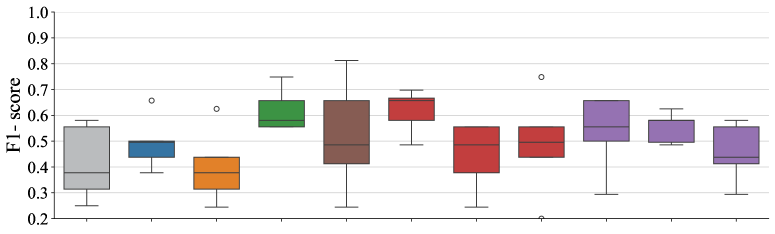
(a) Test F1-score on ACL injury data.

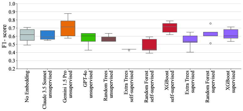
(b) Test F1-score on post-trauma pain data.

Figure 3: Test F1-score at 67%/33% train/test splits of a linear model without embeddings, with our LLM-based zero-shot decision tree embeddings, as well as with unsupervised, self-supervised, and supervised embedding baselines on our private (a) ACL injury data and (b) post-trauma pain data.

The results for the median test F1-score for our induction experiments can be found in Table 1 and the test balanced accuracy results in Table 4 in Appendix C. Figure 7(a) in Appendix C shows the statistical significance of our findings. Figure 2 and Figure 4 in Appendix C show test F1-score boxplots and test balanced accuracy boxplots for our private datasets, respectively.

On the public data, our knowledge-driven trees achieved a competitive performance to data-driven trees on individual datasets - without having seen any of the training data. At 67%/33% train/test splits, for instance, Gemini 1.5 Pro achieved a better median test balanced accuracy to OCTs on labor (+0.05) and Claude 3.5 Sonnet even reached a better score than both data-driven interpretable baselines on boxing1 (+0.05 and + 0.09). On our ACL injury data, the data-driven interpretable baselines only achieved a median test balanced accuracy and F1-score $\leq$ 0.50 at 67%/33% train/test splits, and were surpassed by Claude Sonnet 3.5 with a median test balanced accuracy of 0.59 as well as GPT-4o with a median test balanced accuracy of 0.55 and an F1-score of 0.63. On our post-trauma pain data, the data-driven interpretable baselines achieved a median test balanced accuracy $\leq$ 0.56 at 67%/33% train/test splits, and were outperformed by Claude 3.5 Sonnet with a median score of 0.62. Claude 3.5 Sonnet achieved a median test F1-score of 0.86, the same as BSS and slightly lower than OCTs. Please refer to Appendix C for results on the predictive performance at different train/test splits and for details on the overall best trees for our private data.

Decision Tree Embedding Results

The median test F1-score results for our embedding experiments can be found in Table 2, the test balanced accuracy results in Table 5 in Appendix C. Figure 7(b) in Appendix C shows the statistical significance of our findings. Figure 3 and Figure 6 in Appendix C show test F1-score boxplots and test balanced accuracy boxplots for our private datasets.

On the public data, our LLM-based zero-shot embeddings narrowed the gap to the data-driven decision tree induction. The median test F1-score difference to OCTs decreased by +0.08 for Claude 3.5 Sonnet, by +0.23 for Gemini 1.5 Pro, and by +0.22 for GPT-4o. Similarly, the median test balanced accuracy difference to OCTs decreased by +0.20 for Claude 3.5 Sonnet, by +0.24 for Gemini 1.5 Pro, and by +0.25 for GPT-4o. Our zero-shot embeddings were on par with, i.e., not statistically different from, the best self-supervised and supervised embeddings (Figure 7(b) in Appendix C), and surpassed unsupervised random trees embeddings by at least +0.06 and +0.06 in terms of median test F1-score and balanced accuracy. On individual datasets, the median test F1-score and balanced accuracy improved compared to no embedding by up to +0.33 and +0.30. On our ACL injury data, GPT-4o increased the median test F1-score and balanced accuracy compared to no embedding by +0.20 and +0.20 and was only outperformed by self-supervised extra trees embeddings with improvements of +0.28 and +0.30, respectively. Unsupervised random trees embeddings only showed much smaller improvements of +0.11 and +0.10. On our post-trauma pain data, the embeddings by Gemini 1.5 Pro and self-supervised XGBoost were the only ones to demonstrate a performance improvement compared to no embedding, with increases of +0.10 and +0.10 in median test F1-score and +0.11 and +0.07 in median test balanced accuracy, respectively. Please refer to Appendix C for more insights regarding the dimensionality of our embeddings, the selected feature variability, as well as the effect of changing the decision forest size and concatenating our embeddings to the original feature vectors.

7 Conclusion

LLMs provide powerful means to leverage prior knowledge in the low-data regime. In this work, we presented how we can use the condensed world knowledge within state-of-the-art LLMs to induce decision trees without any training data. We showed that these zero-shot trees can even surpass data-driven trees on some small-sized tabular datasets, while remaining intrinsically interpretable and privacy-preserving. Additionally, we demonstrated how we can generate knowledge-driven embeddings using our zero-shot trees and combine them with downstream models to infuse prior knowledge into data-driven approaches, with a predictive performance that matches data-driven tree-based embeddings on average. We therefore argue that our tree induction and embedding approaches can serve as strong new baselines for data-driven machine learning methods.

Nevertheless, we want to point out that our conclusions are so far based on small-sized tabular classification datasets and do not necessarily extend to other settings. We also focused on a simple prompting template that could be adapted for better performance (Dong et al. 2024; Nori et al. 2023; Schulhoff et al. 2024), e.g., by enriching the prompts with additional information from standards, guidelines, or research papers. We also expect further performance boosts with the rise of even more powerful LLMs (OpenAI 2024c), and by iteratively improving our zero-shot trees with training data (Chao et al. 2024; Eiben and Smith 2015; Nam et al. 2024; Ryan, O’Neill, and Collins 2018; Snell et al. 2024). Alternatively, our trees could be used to obtain probabilistic outputs, e.g., by counting the fraction of training examples in each leaf. Even different probabilistic classifiers like logistic regression could potentially be generated following our general template (Garg et al. 2022; Grazzi et al. 2024). Overall, we believe that leveraging LLMs as zero-shot model generators opens up a new toolbox for practitioners and researchers to tailor LLM-based machine learning models to their needs.

Appendix A Dataset Selection Criteria

We selected all small-sized tabular datasets from the public Penn Machine Learning Benchmarks (PMLB) (Olson et al. 2017; Romano et al. 2022) that fulfilled the following criteria:

• The sample size was $\leq 500$. This allowed us to test our zero-shot decision trees in a setting where data-driven machine learning methods often struggle (Christodoulou et al. 2019; Knauer, Grimm, and Rodner 2024; McElfresh et al. 2024) and knowledge-driven or -guided approaches show great promise for predictive modeling (Harrell 2015; Heinze, Wallisch, and Dunkler 2018; Knauer and Rodner 2023).

• The dataset covered a classification problem. Regression problems (that are not piecewise linear) typically require deeper trees that are much less interpretable, removing one of the key advantages that decision trees have over other machine learning methods.

• A data-driven decision tree classifier (Bertsimas and Dunn 2017) with a maximum depth of up to 2 could achieve a training F1-score $\geq 0.8$ on the dataset. This ensured that a shallow decision tree was indeed a reasonable model for the data.

• The feature names were informative. As our induction and embedding approaches rely on the feature names to derive decision rules, names like “xs” and “ys” cannot be expected to yield meaningful zero-shot trees.

With these criteria, we arrived at 14 public datasets. We excluded the iris dataset, though, because we employed it in our prompt template (Listing 1), yielding a total of 13 public datasets for our evaluation.

Appendix B Additional Dataset Details

In the following, we provide more information on the 13 public and 2 private datasets used for our evaluation.

Public Datasets

For our 13 public datasets, we used tabmemcheck 0.1.5 to evaluate whether state-of-the-art LLMs know or have memorized them, i.e., we assessed the LLMs’ knowledge of the feature names with the feature names test, the memorization of the table header with the header test, the memorization of 25 random rows with the row completion test, the memorization of 25 unique feature values with the feature completion test, and the memorization of the first tokens from 25 random rows with the first token test (Bordt, Nori, and Caruana 2024; Bordt et al. 2024). The test results are shown in Table 3, together with the sample sizes, feature set sizes, and number of classes. We found evidence of knowledge (54%) or partial memorization (62%) of the public datasets by at least 1 state-of-the-art LLM. Our LLM-based decision tree induction and embedding approaches may therefore show overoptistmic performance results on these datasets.

Dataset	Sample size	Feature set size	Number of classes	Feature names test	Header test	Row completion test	Feature completion test	First token test
bankruptcy	50	6	2	? / $\times$ / ?	$\times$ / $\times$ / $\times$	$\times$ / $\times$ / $\times$	$\times$ / - / $\times$	$\times$ / - / $\times$
japansolvent	52	9	2	$\times$ / $\times$ / $\times$	$\times$ / $\times$ / $\times$	$\times$ / $\times$ / $\times$	$\times$ / $\times$ / $\times$	? / ✓/ ✓
labor	57	16	2	✓/ ✓/ ✓	? / $\times$ / $\times$	$\times$ / $\times$ / $\times$	? / ? / ?	$\times$ / $\times$ / $\times$
creditscore	100	6	2	? / $\times$ / $\times$	$\times$ / $\times$ / $\times$	$\times$ / $\times$ / $\times$	$\times$ / $\times$ / $\times$	$\times$ / ? / $\times$
boxing1	120	3	2	$\times$ / - / $\times$	? / ? / ?	✓ ✓/ ✓	$\times$ / $\times$ / $\times$	✓/ - / ✓
boxing2	132	3	2	$\times$ / - / $\times$	? / ? / ✓	✓/ ✓/✓	$\times$ / $\times$ / $\times$	✓/ ✓/ ✓
hepatitis	155	19	2	✓/ ✓/ ✓	✓/ ? / ?	$\times$ / $\times$ / $\times$	? / $\times$ / $\times$	$\times$ / $\times$ / $\times$
heart_h	294	13	2	✓/ ✓/ ✓	✓/ ? / $\times$	✓/ $\times$ / $\times$	? / $\times$ / $\times$	- / - / -
penguins	344	7	3	✓/ ✓/ ✓	✓/ ✓/ ✓	✓/ $\times$ / $\times$	$\times$ / $\times$ / $\times$	$\times$ / ✓/ -
colic	368	22	2	? / ? / ✓	$\times$ / $\times$ / $\times$	$\times$ / $\times$ / $\times$	$\times$ / $\times$ / $\times$	- / - / -
house_votes_84	435	16	2	✓/ - / ✓	✓/ ? / ?	$\times$ / $\times$ / $\times$	✓/ ? / ✓	- / ? / $\times$
vote	435	16	2	✓/ - / ✓	✓/ ? / ?	$\times$ / $\times$ / $\times$	✓/ ? / ✓	- / ? / $\times$
irish	500	5	2	$\times$ / $\times$ / $\times$	? / ? / ?	$\times$ / $\times$ / $\times$	$\times$ / $\times$ / $\times$	- / - / -

Table 3: Additional dataset details for our 13 public datasets, including the sample sizes, the feature set sizes, the number of classes, and tests evaluating whether state-of-the-art LLMs know or have memorized our public datasets (Bordt, Nori, and Caruana 2024; Bordt et al. 2024). The knowledge and memorization test results for Anthropic Claude 3.5 Sonnet, Google Gemini 1.5 Pro, and OpenAI GPT-4o are depicted in the table as * / * / *, with “✓”, “$\times$”, “?”, and “-” denoting “evidence of knowledge or memorization”, “no evidence of knowledge or memorization”, “ambiguous result”, and “test could be conducted”, respectively.

Private Datasets

To obtain unbiased performance estimates, we additionally included 2 private datasets that are not publicly available and hence cannot have been seen during the LLMs’ pretraining (Bordt, Nori, and Caruana 2024; Bordt et al. 2024).

Post-Trauma Pain

The first private dataset is from a recent prospective cohort study in 124 post-trauma patients (Evans et al. 2022). The prediction target $p$ was to classify “whether the pain and disability outcome at 6 months following musculoskeletal trauma is good or bad”. At 6 months, there were 82 follow-up responders. The baseline set of 40 predictors included surrogates for pain mechanisms, qualitative sensory testing, and psychosocial factors, among others. We regarded the gender at birth, ethnicity, education age, work status, and penetrating injury as nominal, and the smoke status and injury severity score category as ordinal. Ordinal predictors were treated as numerical in our experiments (Steyerberg 2019). Missing values ranged from 0% to 30% per feature, with a mean of 5% and a median of 1%. For more details on the dataset, please refer to the original publication.

Anterior Cruciate Ligament Injury

The second private dataset is from a to-be-published prospective cohort study in 34 patients with an ACL rupture (Brisson et al. 2020, 2024). The prediction target $p$ was to classify “whether the cartilage thickness change in the central medial femur over 12 months following anterior cruciate ligament injury is normal or abnormal”. Patients were assessed at a baseline of 5 months post-injury (± unbiased standard deviation estimate (SD) 3 months) and at a follow-up of 12 months (±SD 1 month). At baseline, we collected 3-dimensional gait data using a 10-camera motion capture system (Vicon) and 2 force plates (AMTI) during barefoot, overground walking at a natural, self-selected speed. Using the gait data and inverse dynamics (Winter 2009), we computed external peak knee moments in a 3-dimensional floating axis coordinate system (Wu and Cavanagh 1995). At both baseline and 12-months follow-up, we performed magnetic resonance imaging (MRI) with a 1.5 Tesla scanner (Avanto, Siemens; sagittal multi-echo spin-echo (MESE); 3.50mm slice spacing; 0.31mm in-plane resolution) to compute tibiofemoral, subregional mean cartilage thickness (Wirth and Eckstein 2008) and measures of cartilage composition, i.e., mean superficial and deep cartilage transverse relaxation times (T2), 50% each (Wirth, Maschek, and Eckstein 2017). We were primarily interested in excessive cartilage thinning or thickening in the central medial femur over 12 months (Biswal et al. 2002; Frobell et al. 2009) as a potential precursor to osteoarthritis (Iriondo et al. 2021). We considered a cartilage thickness change abnormal in our experiments if it exceeded 1 SD of 13 healthy controls (0.03mm ±SD 0.07mm). The set of 20 baseline predictors included external peak knee moments, baseline mean cartilage thickness in the central medial femur, measures of cartilage composition in the central medial femur, patient-reported outcome measures, and a group assignment into copers (treated conservatively and clinically deemed to have mechanically stable knees), noncopers (treated conservatively and clinically deemed to have persistent mechanical knee instability), and surgical reconstruction (ipsilateral four-strand semitendinosus reconstruction, 4 months post-injury ±SD 3 months) (Kaplan 2011; Thoma et al. 2019), among others. We regarded the group assignment, sex, and dominant leg as nominal, and the Tegner score as ordinal. The Tegner score was treated as numerical in our experiments (Steyerberg 2019). There were no missing values in this dataset.

Appendix C Additional Results

	Ours			Interpretable models		AutoML and deep learning
Dataset	Claude 3.5 Sonnet	Gemini 1.5 Pro	GPT-4o	BSS	OCTs	Auto-Gluon	Auto-Prognosis	TabPFN
public median	0.59	0.54	0.54	0.75	0.82	0.83	0.89	0.88
bankruptcy	0.62	0.65	0.71	0.90	0.83	0.90	0.92	0.92
boxing1	0.59	0.44	0.50	0.54	0.50	0.69	0.69	0.67
boxing2	0.63	0.43	0.46	0.70	0.70	0.68	0.78	0.62
creditscore	0.55	0.48	0.56	0.62	1.00	0.98	1.00	0.90
japansolvent	0.67	0.58	0.52	0.79	0.72	0.83	0.72	0.89
colic	0.36	0.56	0.58	0.81	0.83	0.82	0.81	0.81
heart_h	0.50	0.50	0.25	0.82	0.76	0.79	0.81	0.77
hepatitis	0.62	0.49	0.50	0.63	0.60	0.68	0.71	0.67
house_votes_84	0.16	0.48	0.50	0.95	0.95	0.96	0.96	0.96
irish	0.62	0.56	0.63	0.72	1.00	1.00	1.00	1.00
labor	0.69	0.74	0.67	0.77	0.69	0.74	0.89	0.84
penguins	0.91	0.67	0.84	*	0.98	0.98	0.99	0.99
vote	0.48	0.49	0.53	0.52	0.78	0.95	0.95	0.95
private median	0.60	0.54	0.56	0.53	0.50	0.50	0.60	0.56
ACL injury	0.59	0.50	0.55	0.50	0.50	0.50	0.50	0.56
post-trauma	0.62	0.57	0.58	0.56	0.50	0.50	0.68	0.73

Table 4: Median test balanced accuracy at 67%/33% train/test splits for our LLM-based zero-shot decision tree induction approach compared to the machine learning baselines. The best score among the zero-shot methods is highlighted. *BSS via Interpretable AI 3.1.1 does not support multiclass classifications.

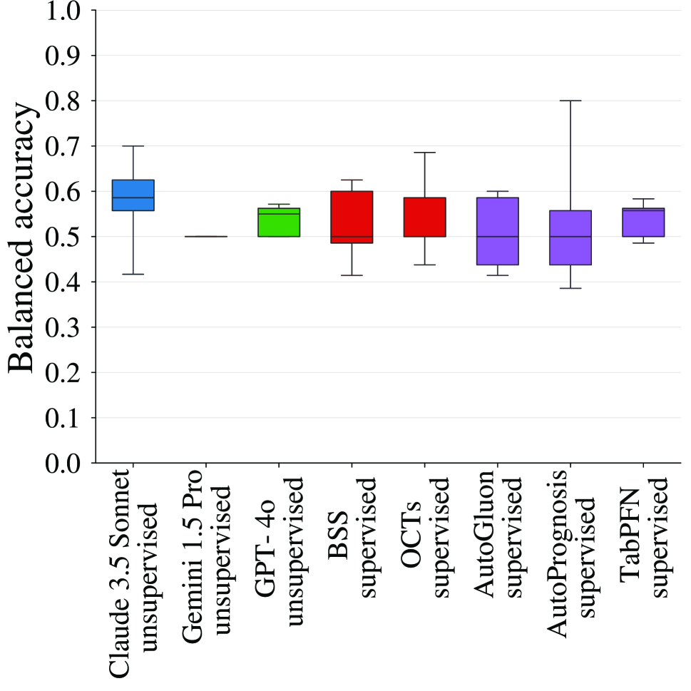
(a) Balanced accuracy on ACL injury data.

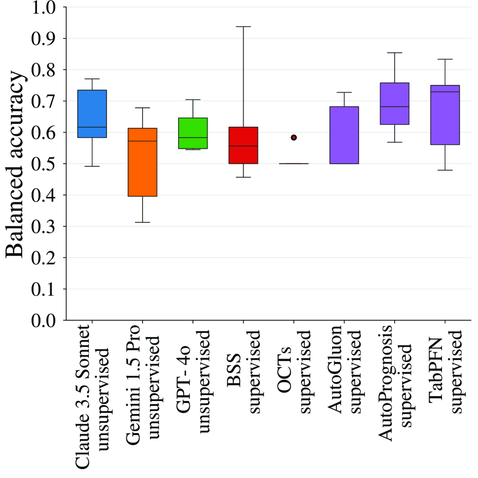
(b) Balanced accuracy on post-trauma pain data.

Figure 4: Test balanced accuracy at 67%/33% train/test splits for our LLM-based zero-shot decision tree induction approach compared to the machine learning baselines on our private (a) ACL injury data and (b) post-trauma pain data.

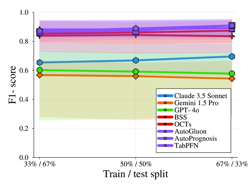
(a) F1-score on public data.

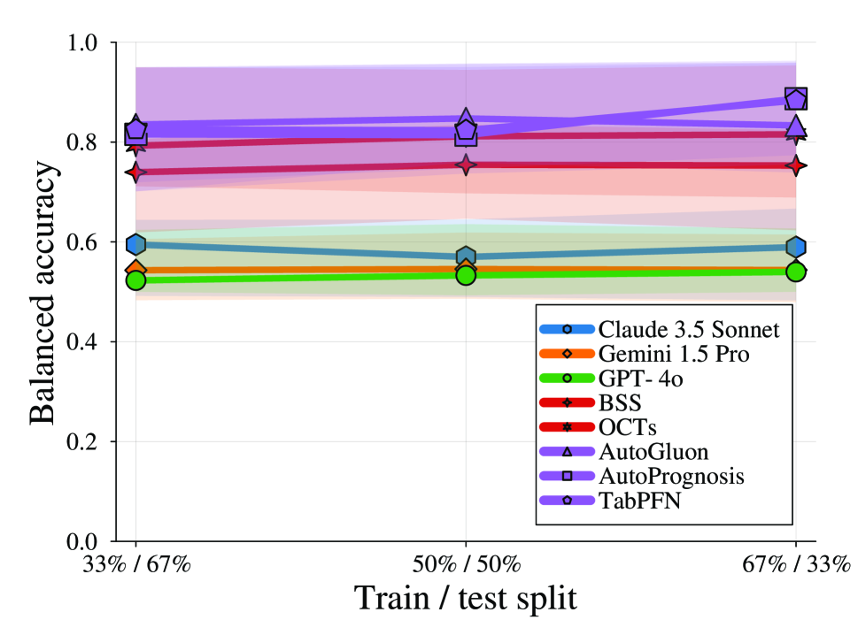
(b) Balanced accuracy on public data.

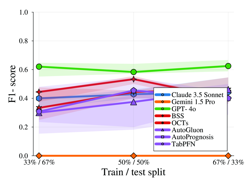
(c) F1-score on ACL injury data.

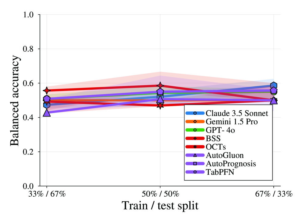
(d) Balanced accuracy on ACL injury data.

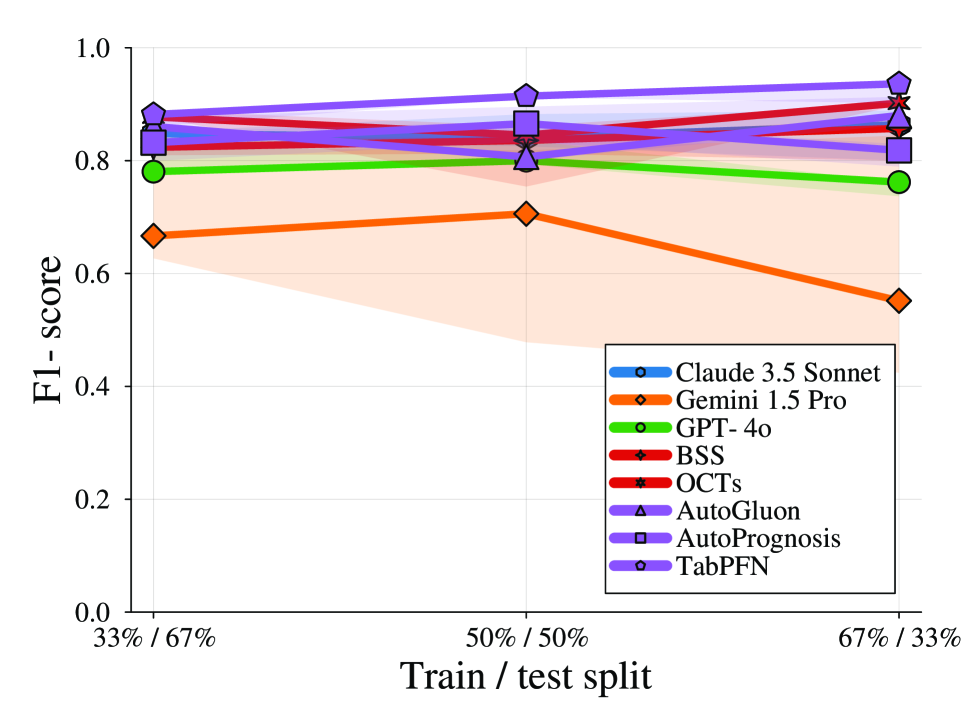
(e) F1-score on post-trauma pain data.

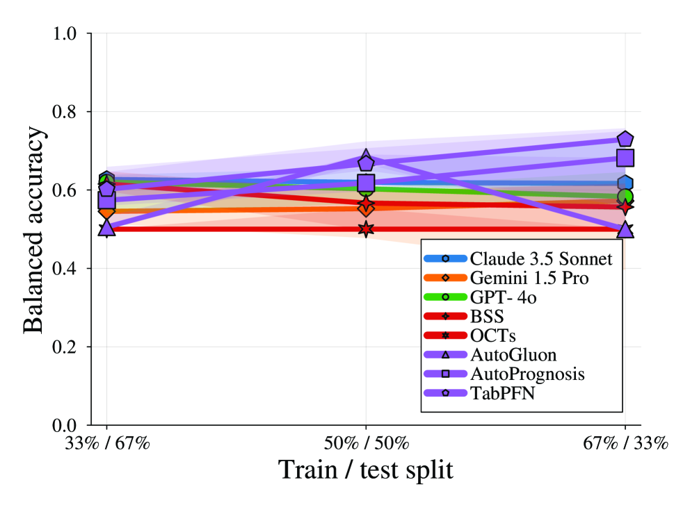
(f) Balanced accuracy on post-trauma pain data.

Figure 5: Test medians and interquartile ranges at different train/test splits for our LLM-based zero-shot decision tree induction approach compared to the machine learning baselines on our (a) public data, (b) private ACL injury data, and (c) private post-trauma pain data.

		Ours			Unsupervised	Self-supervised			Supervised
Dataset	No embedding	Claude 3.5 Sonnet	Gemini 1.5 Pro	GPT-4o	Ran-dom trees	Extra trees	Ran-dom forest	XG-Boost	Extra trees	Ran-dom forest	XG-Boost
public median	0.78	+0.01	0.00	+0.01	-0.06	-0.13	-0.23	0.00	-0.04	+0.05	+0.02
bankruptcy	0.94	-0.06	-0.16	-0.06	-0.18	-0.11	-0.06	-0.11	-0.12	-0.11	-0.06
boxing1	0.64	+0.02	-0.05	+0.05	+0.04	-0.07	-0.09	+0.09	-0.04	-0.05	+0.09
boxing2	0.61	+0.16	+0.13	+0.15	+0.04	+0.04	-0.09	+0.01	+0.01	+0.10	+0.06
creditscore	0.74	-0.12	-0.12	-0.10	-0.12	+0.24	+0.22	-0.22	-0.07	+0.24	+0.24
japansolvent	0.83	0.00	-0.06	-0.11	-0.11	-0.33	-0.33	-0.11	0.00	0.00	-0.06
colic	0.80	-0.26	-0.01	+0.01	-0.13	-0.29	-0.30	-0.02	-0.06	-0.02	0.00
heart_h	0.78	+0.01	-0.01	0.00	-0.06	-0.28	-0.28	+0.02	-0.01	0.00	-0.03
hepatitis	0.72	-0.07	-0.09	0.00	-0.08	-0.22	-0.24	-0.08	-0.05	-0.15	-0.05
house_votes_84	0.96	-0.01	-0.02	0.00	-0.02	-0.06	-0.06	0.00	-0.01	-0.02	0.00
irish	0.77	+0.03	+0.21	+0.18	+0.18	-0.08	-0.11	+0.19	+0.06	+0.15	+0.23
labor	0.93	-0.20	-0.21	-0.14	-0.11	-0.23	-0.21	-0.04	-0.18	-0.10	-0.18
penguins	1.00	0.00	0.00	0.00	-0.04	-0.32	-0.39	-0.33	-0.11	-0.09	-0.02
vote	0.53	+0.26	+0.26	+0.30	+0.10	-0.01	+0.01	+0.27	+0.08	+0.26	+0.26
private median	0.51	+0.05	+0.05	+0.08	0.00	+0.08	-0.02	+0.11	+0.05	+0.08	+0.02
ACL injury	0.39	+0.13	0.00	+0.20	+0.10	+0.30	+0.10	+0.14	+0.17	+0.20	+0.07
post-trauma	0.64	-0.02	+0.11	-0.04	-0.10	-0.14	-0.14	+0.07	-0.07	-0.04	-0.04

Table 5: Median test balanced accuracy at 67%/33% train/test splits of a linear model without embeddings (first column). Subsequent columns display the performance difference of our LLM-based zero-shot decision tree embedding approach as well as the unsupervised, self-supervised, and supervised embedding baselines relative to the first column. If there is an improvement compared to no embedding, the best score among the unsupervised methods is highlighted.

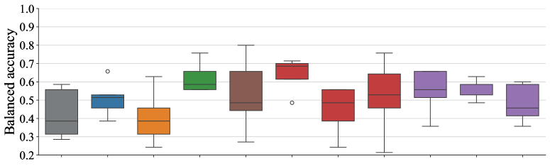
(a) Test balanced accuracy on ACL injury data.

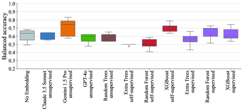
(b) Test balanced accuracy on post-trauma pain data.

Figure 6: Test balanced accuracy at 67%/33% train/test splits of a linear model without embeddings, with our LLM-based zero-shot decision tree embeddings, as well as with unsupervised, self-supervised, and supervised embedding baselines on our private (a) ACL injury data and (b) post-trauma pain data.

(a) Test F1-score ranks (left) and test balanced accuracy ranks (right) for our zero-shot decision tree induction experiments.

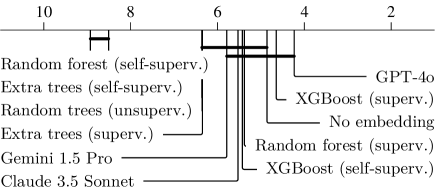
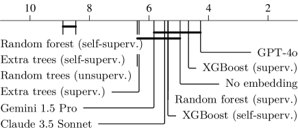
(b) Test F1-score ranks (left) and test balanced accuracy ranks (right) for our zero-shot decision tree embedding experiments.

Figure 7: Critical difference diagrams to detect pairwise test score differences between our methods at 67%/33% train/test splits for the public and private datasets, based on the Holm-adjusted Wilcoxon signed-rank test (Benavoli, Corani, and Mangili 2016; Demšar 2006). Approaches that are not statistically different at the 0.05 significance level are connected by a bold horizontal bar. Missing performance scores were imputed with 0 before running the tests.

Dataset	Feature set size	Claude 3.5 Sonnet	Gemini 1.5 Pro	GPT-4o
bankruptcy	6	30	22	26
boxing1	3	28	21	24
boxing2	3	30	24	26
creditscore	6	30	22	29
japansolvent	9	30	21	25
colic	22	35	46	35
heart_h	13	35	16	26
hepatitis	19	35	25	27
house_votes_84	16	32	20	30
irish	5	30	20	30
labor	16	30	20	30
penguins	7	30	18	27
vote	16	30	21	29
ACL injury	20	33	20	30
post-trauma	40	32	58	20

Table 6: Embedding dimension for our zero-shot decision forests, consisting of 5 decision trees generated by the 3 LLMs.

Dataset	Feature set size	Claude 3.5 Sonnet	Gemini 1.5 Pro	GPT-4o
bankruptcy	6	5	5	5
boxing1	3	3	3	3
boxing2	3	3	3	3
creditscore	6	6	6	6
japansolvent	9	8	7	8
colic	22	10	13	21
heart_h	13	12	9	13
hepatitis	19	12	17	19
house_votes_84	16	16	15	16
irish	5	4	5	5
labor	16	16	15	16
penguins	7	6	6	6
vote	16	14	16	15
ACL injury	20	17	10	16
post-trauma	40	32	18	20

Table 7: Number of features selected by the 3 LLMs in their 5 generated decision trees.

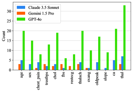
Figure 8: Count of feature usages in the embedding for the heart_h dataset, noting that some of the 5 generated decision trees use the same feature multiple times.

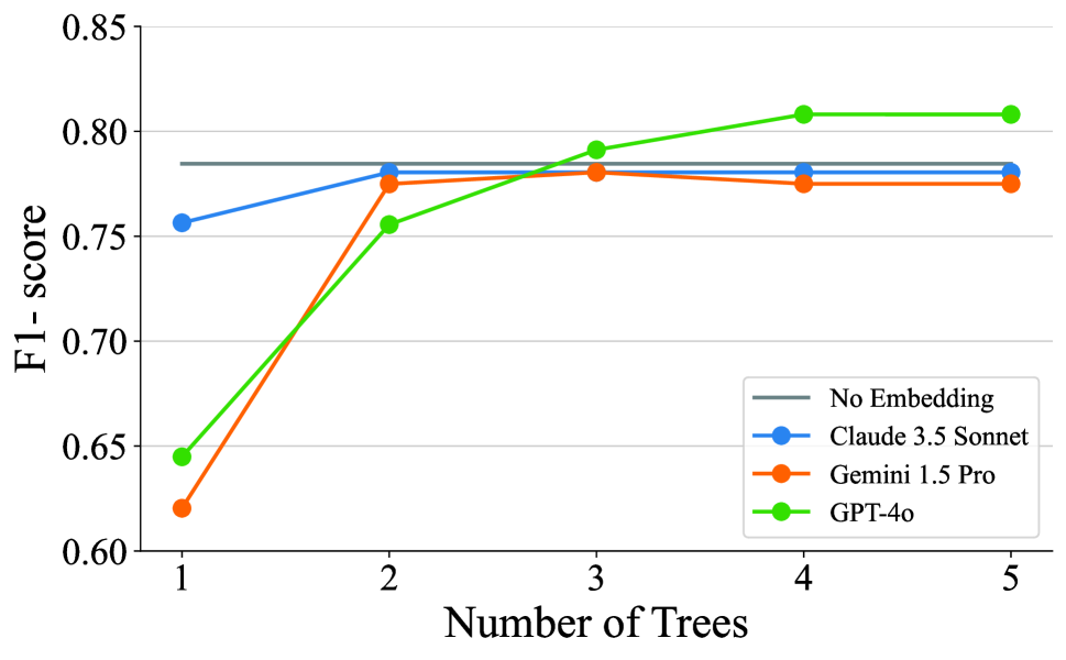
(a) Median test F1-score.

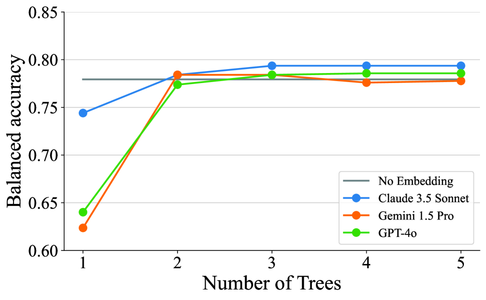
(b) Median test balanced accuracy.

Figure 9: Median test (a) F1-score and (b) balanced accuracy at 67%/33% train/test splits across the 13 public datasets for varying LLM-based zero-shot decision forest embedding sizes.

In this section, we present additional experimental results. Table 4, Figure 4, and Figure 5 show further results for our zero-shot decision tree induction, Table 5 and Figure 6 for our zero-shot decision tree embedding. Figure 7 shows the statistical significance of our findings via critical difference diagrams (Benavoli, Corani, and Mangili 2016; Demšar 2006). Furthermore, we provide additional details on the overall best trees for the private datasets and our zero-shot embeddings below.

Best Induced Trees on Private Datasets

On our ACL injury data, the overall best tree was built by GPT-4o, with a test balanced accuracy of 0.56 and an F1-score of 0.78, and it included the baseline mean cartilage thickness in the central medial femur as a feature (like all trees built by GPT-4o) as well as the International Knee Documentation Committee (IKDC) score. At different train/test splits, the median test F1-score for GPT-4o also remained higher than for the data-driven interpretable baselines (Figure 5), although the overall best tree could vary depending on the split.

On our post-traum pain data, the overall best tree was built by Claude 3.5 Sonnet. With a test balanced accuracy of 0.73 and an F1-score of 0.89, it even matched the performance in the original publication (Evans et al. 2022), but without having used any training data. It included the average pain intensity (as in Evans et al. 2022), the Short Form 36 (SF-36) physical component summary, and the pain self-efficacy questionnaire (PSEQ) score. At different train/test splits, the median rankings remained mostly stable (Figure 5), with Claude 3.5 Sonnet consistently showing the overall best decision tree induction performance across splits.

Additional Embedding Insights

Table 6 shows the dimensions of the zero-shot embeddings generated by the 3 LLMs. In general, the LLM-based embeddings increased the dataset dimensionality, except the Gemini 1.5 Pro embedding for our ACL injury data as well as the Claude 3.5 Sonnet and GPT-4o embeddings for our post-trauma pain data. However, the embedding size varied significantly across the datasets when no constraints were applied, suggesting that different maximum tree depths were chosen by the LLMs. When considering the results in Table 2 and Table 5, though, no clear correlation between the embedding size and performance could be established. For instance, on the irish dataset, Claude 3.5 Sonnet and GPT-4o had embedding dimensions of 30, Gemini 1.5 Pro of 20. Nevertheless, Claude 3.5 Sonnet only showed a minimal improvement of +0.01 in the median test F1-score compared to no embedding, while GPT-4o and Gemini 1.5 Pro exhibited much larger improvements of +0.18 and +0.21, respectively.

In terms of the number of selected features, we observed that the LLM-based embeddings leveraged a diverse feature set, providing a rich representation of the data. The embeddings resulted in trees with a comparable number of features (Table 7). This consistency in feature usage across different models suggests that the observed performance differences were likely not due to the selection of features, but rather to their combination and the thresholds applied. When considering the total instances of feature usage (noting that some decision trees use the same feature multiple times), it becomes apparent that GPT-4o utilized features much more frequently than Claude 3.5 Sonnet and Gemini 1.5 Pro. Figure 8 illustrates the feature count for the heart_h dataset, as an example.

Finally, the median test F1-score and balanced accuracy results across different decision forest sizes are shown in Figure 9, which indicates that at least 3 trees are necessary to achieve a performance improvement compared to logistic regression without any embedding. Furthermore, the performance seems to saturate after 4 trees, confirming that our default decision forest size of 5 appears to be a reasonable choice.

Embedding Concatenation Approach

In addition to the embedding approach discussed in the main text, we explored an alternative method that combined the embeddings generated via our zero-shot decision trees with the original features vectors. This concatenation approach assumes that the additional information provided by the original features could enhance the performance of our primary embedding approach. However, to isolate the effectiveness of the tree-based embeddings, our primary analysis focused solely on embeddings without the original feature vectors.

To evaluate the performance of the concatenation approach, we conducted a comparative analysis across the 13 public datasets using the median test F1-score (Table 8) and balanced accuracy (Table 9). Overall, adding the original feature vectors slightly improved the performance for all LLMs (Claude 3.5 Sonnet, Gemini 1.5 Pro, and GPT-4o).

Dataset	Claude 3.5 Sonnet	Gemini 1.5 Pro	GPT-4o
public median	+0.04	+0.03	+0.01
bankruptcy	+0.06	+0.18	+0.12
boxing1	+0.04	+0.03	+0.01
boxing2	-0.02	0.00	0.00
creditscore	+0.07	+0.04	+0.12
japansolvent	0.00	+0.05	+0.06
colic	+0.28	+0.03	-0.03
heart_h	+0.01	+0.01	+0.02
hepatitis	+0.07	+0.10	+0.02
house_votes_84	-0.01	+0.01	0.00
irish	+0.01	+0.01	-0.01
labor	+0.13	+0.19	+0.06
penguins	0.00	0.00	0.00
vote	+0.05	+0.06	0.00

Table 8: Test F1-score improvement of the concatenation approach (zero-shot decision tree embeddings + original data) compared to our standalone LLM-based zero-shot decision tree embeddings across the 13 public datasets. The values are the median over 5 random 67%/33% train/test splits.

Dataset	Claude 3.5 Sonnet	Gemini 1.5 Pro	GPT-4o
public median	+0.04	+0.03	+0.01
bankruptcy	+0.06	+0.16	+0.12
boxing1	+0.04	+0.01	0.00
boxing2	-0.02	0.00	0.00
creditscore	+0.10	+0.06	+0.10
japansolvent	0.00	+0.06	+0.06
colic	0.26	+0.03	-0.02
heart_h	0.00	+0.01	+0.02
hepatitis	+0.08	+0.10	+0.01
house_votes_84	-0.01	+0.01	+0.01
irish	0.00	+0.01	-0.01
labor	+0.14	+0.18	+0.07
penguins	0.00	0.00	0.00
vote	+0.05	+0.06	0.00

Table 9: Test balanced accuracy improvement of the concatenation approach (zero-shot decision tree embeddings + original data) compared to our standalone LLM-based zero-shot decision tree embeddings across the 13 public datasets. The values are the median over 5 random 67%/33% train/test splits.

Appendix D Reproducibility Checklist

Unless specified otherwise, please answer “yes” to each question if the relevant information is described either in the paper itself or in a technical appendix with an explicit reference from the main paper. If you wish to explain an answer further, please do so in a section titled “Reproducibility Checklist” at the end of the technical appendix.

1. This paper

   1. Includes a conceptual outline and/or pseudocode description of AI methods introduced (yes/partial/no/NA) [yes] See Sect. 3 and Sect. 4.

   2. Clearly delineates statements that are opinions, hypothesis, and speculation from objective facts and results (yes/no) [yes] See, e.g., Sect. 6 and 7.

   3. Provides well marked pedagogical references for less-familiar readers to gain background necessary to replicate the paper (yes/no) [yes] See Sect. 2.

2. Does this paper make theoretical contributions? (yes/no) [no]

3. Does this paper rely on one or more datasets? (yes/no) [yes]

   1. A motivation is given for why the experiments are conducted on the selected datasets (yes/partial/no/NA) [yes] See Appendix A.

   2. All novel datasets introduced in this paper are included in a data appendix. (yes/partial/no/NA) [no] Our private ACL and post-trauma pain datasets contain sensitive patient information and therefore cannot be shared.

   3. All novel datasets introduced in this paper will be made publicly available upon publication of the paper with a license that allows free usage for research purposes. (yes/partial/no/NA) [no] See above.

   4. All datasets drawn from the existing literature (potentially including authors’ own previously published work) are accompanied by appropriate citations. (yes/no/NA) [yes] See Appendix A.

   5. All datasets drawn from the existing literature (potentially including authors’ own previously published work) are publicly available. (yes/partial/no/NA) [yes] See Appendix B.

   6. All datasets that are not publicly available are described in detail, with explanation why publicly available alternatives are not scientifically satisficing. (yes/ partial/no/NA) [yes] See Appendix B.

4. Does this paper include computational experiments? (yes/no) [yes]

   1. Any code required for pre-processing data is included in the appendix. (yes/partial/no) [yes] See Code Appendix.

   2. All source code required for conducting and analyzing the experiments is included in a code appendix. (yes/ partial/no) [yes] See Code Appendix.

   3. All source code required for conducting and analyzing the experiments will be made publicly available upon publication of the paper with a license that allows free usage for research purposes. (yes/partial/no) [yes]

   4. All source code implementing new methods have comments detailing the implementation, with references to the paper where each step comes from (yes/partial/no) [yes] See Code Appendix.

   5. If an algorithm depends on randomness, then the method used for setting seeds is described in a way sufficient to allow replication of results. (yes/partial/no/NA) [yes] Where possible, random seeds were set explicitly in our source code. Note that random seeds could not be set for, e.g., Gemini 1.5 Pro and Claude 3.5 Sonnet.

   6. This paper specifies the computing infrastructure used for running experiments (hardware and software), including GPU/CPU models; amount of memory; operating system; names and versions of relevant software libraries and frameworks. (yes/partial/no) [yes] See Sect. 5.

   7. This paper formally describes evaluation metrics used and explains the motivation for choosing these metrics. (yes/partial/no) [yes] See Sect. 5.

   8. This paper states the number of algorithm runs used to compute each reported result. (yes/no) [yes] See Sect. 5.

   9. Analysis of experiments goes beyond single-dimensional summaries of performance (e.g., average; median) to include measures of variation, confidence, or other distributional information. (yes/no) [yes] See Sect. 6 and Appendix C.

   10. The significance of any improvement or decrease in performance is judged using appropriate statistical tests (e.g., Wilcoxon signed-rank). (yes/partial/no) [yes] See Sect. 6 and Appendix C.

   11. This paper lists all final (hyper-)parameters used for each model/algorithm in the paper’s experiments. (yes/partial/no/NA) [yes] See Sect. 5.

   12. This paper states the number and range of values tried per (hyper-) parameter during development of the paper, along with the criterion used for selecting the final parameter setting. (yes/partial/no/NA) [yes] See Sect. 5.

References

- Alaa and Schaar (2018) Alaa, A.; and Schaar, M. 2018. Autoprognosis: Automated clinical prognostic modeling via bayesian optimization with structured kernel learning. In Proceedings of the 35th International Conference on Machine Learning (ICML), 139–148. PMLR.
- Anthropic (2024a) Anthropic. 2024a. The Claude 3 model family: Opus, Sonnet, Haiku. Claude 3 Model Card.
- Anthropic (2024b) Anthropic. 2024b. Data Processing Addendum. https://www.anthropic.com/legal/commercial-terms. Accessed: 2024-07-01.
- Banko and Brill (2001) Banko, M.; and Brill, E. 2001. Scaling to very very large corpora for natural language disambiguation. In Proceedings of the 39th annual meeting of the Association for Computational Linguistics, 26–33.
- Benavoli, Corani, and Mangili (2016) Benavoli, A.; Corani, G.; and Mangili, F. 2016. Should we really use post-hoc tests based on mean-ranks? The Journal of Machine Learning Research, 17(1): 152–161.
- Bertsimas and Dunn (2017) Bertsimas, D.; and Dunn, J. 2017. Optimal classification trees. Machine Learning, 106: 1039–1082.
- Bertsimas, Pauphilet, and Van Parys (2021) Bertsimas, D.; Pauphilet, J.; and Van Parys, B. 2021. Sparse classification: a scalable discrete optimization perspective. Machine Learning, 110: 3177–3209.
- Bertsimas, Pawlowski, and Zhuo (2018) Bertsimas, D.; Pawlowski, C.; and Zhuo, Y. D. 2018. From predictive methods to missing data imputation: an optimization approach. Journal of Machine Learning Research, 18(196): 1–39.
- Biswal et al. (2002) Biswal, S.; Hastie, T.; Andriacchi, T. P.; Bergman, G. A.; Dillingham, M. F.; and Lang, P. 2002. Risk factors for progressive cartilage loss in the knee: a longitudinal magnetic resonance imaging study in forty-three patients. Arthritis & Rheumatism: Official Journal of the American College of Rheumatology, 46(11): 2884–2892.
- Bordt, Nori, and Caruana (2024) Bordt, S.; Nori, H.; and Caruana, R. 2024. Elephants Never Forget: Testing Language Models for Memorization of Tabular Data. arXiv:2403.06644.
- Bordt et al. (2024) Bordt, S.; Nori, H.; Rodrigues, V.; Nushi, B.; and Caruana, R. 2024. Elephants Never Forget: Memorization and Learning of Tabular Data in Large Language Models. arXiv:2404.06209.
- Borisov et al. (2023) Borisov, V.; Broelemann, K.; Kasneci, E.; and Kasneci, G. 2023. DeepTLF: robust deep neural networks for heterogeneous tabular data. International Journal of Data Science and Analytics, 16(1): 85–100.
- Breiman (2001) Breiman, L. 2001. Random forests. Machine learning, 45: 5–32.
- Brisson et al. (2020) Brisson, N. M.; Krahl, L. A. N.; Wirth, W.; Eckstein, F.; and Duda, G. N. 2020. Knee Cartilage Thickness of ACL-Injured Non-Copers & Copers: A 1-Year Study. In Proceedings of the 14th International Workshop on Osteoarthritis Imaging. International Society of Osteoarthritis Imaging.
- Brisson et al. (2024) Brisson, N. M.; Krahl, L. A. N.; Wirth, W.; Eckstein, F.; and Duda, G. N. 2024. Knee Cartilage Transverse Relaxation Time (T2) in Patients with Anterior Cruciate Ligament Injury Treated Conservatively with Structured Physical Rehabilitation or Standard of Care. In Proceedings of the 70th Annual Meeting of the Orthopaedic Research Society. Orthopaedic Research Society.
- Brown et al. (2020) Brown, T.; Mann, B.; Ryder, N.; Subbiah, M.; Kaplan, J. D.; Dhariwal, P.; Neelakantan, A.; Shyam, P.; Sastry, G.; Askell, A.; et al. 2020. Language models are few-shot learners. Advances in neural information processing systems, 33: 1877–1901.
- Chao et al. (2024) Chao, W.; Zhao, J.; Jiao, L.; Li, L.; Liu, F.; and Yang, S. 2024. When large language models meet evolutionary algorithms. arXiv:2401.10510.
- Chen and Guestrin (2016) Chen, T.; and Guestrin, C. 2016. Xgboost: A scalable tree boosting system. In Proceedings of the 22nd ACM SIGKDD international conference on knowledge discovery and data mining, 785–794.
- Chiang et al. (2024) Chiang, W.-L.; Zheng, L.; Sheng, Y.; Angelopoulos, A. N.; Li, T.; Li, D.; Zhang, H.; Zhu, B.; Jordan, M.; Gonzalez, J. E.; and Stoica, I. 2024. Chatbot Arena: An Open Platform for Evaluating LLMs by Human Preference. arXiv:2403.04132.
- Christodoulou et al. (2019) Christodoulou, E.; Ma, J.; Collins, G. S.; Steyerberg, E. W.; Verbakel, J. Y.; and Van Calster, B. 2019. A systematic review shows no performance benefit of machine learning over logistic regression for clinical prediction models. Journal of clinical epidemiology, 110: 12–22.
- Demšar (2006) Demšar, J. 2006. Statistical comparisons of classifiers over multiple data sets. The Journal of Machine learning research, 7: 1–30.
- Dong et al. (2024) Dong, Q.; Li, L.; Dai, D.; Zheng, C.; Ma, J.; Li, R.; Xia, H.; Xu, J.; Wu, Z.; Chang, B.; Sun, X.; Li, L.; and Sui, Z. 2024. A Survey on In-context Learning. arXiv:2301.00234.
- Eiben and Smith (2015) Eiben, A. E.; and Smith, J. E. 2015. Introduction to evolutionary computing. Springer.
- Erickson et al. (2020) Erickson, N.; Mueller, J.; Shirkov, A.; Zhang, H.; Larroy, P.; Li, M.; and Smola, A. 2020. AutoGluon-Tabular: Robust and Accurate AutoML for Structured Data. arXiv:2003.06505.
- Evans et al. (2022) Evans, D. W.; Rushton, A.; Middlebrook, N.; Bishop, J.; Barbero, M.; Patel, J.; and Falla, D. 2022. Estimating risk of chronic pain and disability following musculoskeletal trauma in the United Kingdom. JAMA network open, 5(8): e2228870–e2228870.
- Frobell et al. (2009) Frobell, R.; Le Graverand, M.-P.; Buck, R.; Roos, E.; Roos, H.; Tamez-Pena, J.; Totterman, S.; and Lohmander, L. 2009. The acutely ACL injured knee assessed by MRI: changes in joint fluid, bone marrow lesions, and cartilage during the first year. Osteoarthritis and cartilage, 17(2): 161–167.
- Fu et al. (2024) Fu, D.; Chen, T.-Q.; Jia, R.; and Sharan, V. 2024. Transformers Learn Higher-Order Optimization Methods for In-Context Learning: A Study with Linear Models. arXiv:2310.17086.
- Gallifant et al. (2024) Gallifant, J.; Chen, S.; Moreira, P.; Munch, N.; Gao, M.; Pond, J.; Celi, L. A.; Aerts, H.; Hartvigsen, T.; and Bitterman, D. 2024. Language Models are Surprisingly Fragile to Drug Names in Biomedical Benchmarks. arXiv:2406.12066.
- Garg et al. (2022) Garg, S.; Tsipras, D.; Liang, P. S.; and Valiant, G. 2022. What can transformers learn in-context? a case study of simple function classes. Advances in neural information processing systems, 35: 30583–30598.
- Geurts, Ernst, and Wehenkel (2006) Geurts, P.; Ernst, D.; and Wehenkel, L. 2006. Extremely randomized trees. Machine learning, 63: 3–42.
- Google (2024a) Google. 2024a. Cloud Data Processing Addendum. https://cloud.google.com/terms/data-processing-addendum. Accessed: 2024-07-01.
- Google (2024b) Google. 2024b. Gemini 1.5: Unlocking multimodal understanding across millions of tokens of context. arXiv:2403.05530.
- Grazzi et al. (2024) Grazzi, R.; Siems, J.; Schrodi, S.; Brox, T.; and Hutter, F. 2024. Is Mamba Capable of In-Context Learning? arXiv:2402.03170.
- Halevy, Norvig, and Pereira (2009) Halevy, A.; Norvig, P.; and Pereira, F. 2009. The unreasonable effectiveness of data. IEEE intelligent systems, 24(2): 8–12.
- Harrell (2015) Harrell, F. E. 2015. Regression modeling strategies: with applications to linear models, logistic regression, and survival analysis. Springer.
- He and Ma (2013) He, H.; and Ma, Y. 2013. Imbalanced learning: foundations, algorithms, and applications. John Wiley & Sons.
- Heinze, Wallisch, and Dunkler (2018) Heinze, G.; Wallisch, C.; and Dunkler, D. 2018. Variable selection–a review and recommendations for the practicing statistician. Biometrical journal, 60(3): 431–449.
- Hollmann et al. (2023) Hollmann, N.; Müller, S.; Eggensperger, K.; and Hutter, F. 2023. Tabpfn: A transformer that solves small tabular classification problems in a second. In Proceedings of the 11th International Conference on Learning Representations (ICLR).
- Howard and Ruder (2018) Howard, J.; and Ruder, S. 2018. Universal Language Model Fine-tuning for Text Classification. arXiv:1801.06146.
- Imrie et al. (2023) Imrie, F.; Cebere, B.; McKinney, E. F.; and van der Schaar, M. 2023. AutoPrognosis 2.0: Democratizing diagnostic and prognostic modeling in healthcare with automated machine learning. PLOS Digital Health, 2(6): e0000276.
- Iriondo et al. (2021) Iriondo, C.; Liu, F.; Calivà, F.; Kamat, S.; Majumdar, S.; and Pedoia, V. 2021. Towards understanding mechanistic subgroups of osteoarthritis: 8-year cartilage thickness trajectory analysis. Journal of Orthopaedic Research®, 39(6): 1305–1317.
- Kaplan (2011) Kaplan, Y. 2011. Identifying individuals with an anterior cruciate ligament-deficient knee as copers and noncopers: a narrative literature review. Journal of orthopaedic & sports physical therapy, 41(10): 758–766.
- Knauer, Grimm, and Rodner (2024) Knauer, R.; Grimm, M.; and Rodner, E. 2024. PMLBmini: A Tabular Classification Benchmark Suite for Data-Scarce Applications. arXiv:2409.01635.
- Knauer and Rodner (2023) Knauer, R.; and Rodner, E. 2023. Cost-Sensitive Best Subset Selection for Logistic Regression: A Mixed-Integer Conic Optimization Perspective. In Proceedings of the 46th German Conference on Artificial Intelligence (Künstliche Intelligenz), 114–129. Springer.
- Knauer and Rodner (2024) Knauer, R.; and Rodner, E. 2024. Squeezing Lemons with Hammers: An Evaluation of AutoML and Tabular Deep Learning for Data-Scarce Classification Applications. arXiv:2405.07662.
- Kojima et al. (2022) Kojima, T.; Gu, S. S.; Reid, M.; Matsuo, Y.; and Iwasawa, Y. 2022. Large language models are zero-shot reasoners. Advances in neural information processing systems, 35: 22199–22213.
- Li et al. (2023) Li, Q.; Liang, Y.; Diao, Y.; Xie, C.; Li, B.; He, B.; and Song, D. 2023. Tree-as-a-prompt: boosting black-box large language models on few-shot classification of tabular data. https://openreview.net/forum?id=SJTSvRtGsN. Accessed: 2024-07-01.
- Longo et al. (2024) Longo, L.; Brcic, M.; Cabitza, F.; Choi, J.; Confalonieri, R.; Del Ser, J.; Guidotti, R.; Hayashi, Y.; Herrera, F.; Holzinger, A.; et al. 2024. Explainable Artificial Intelligence (XAI) 2.0: A manifesto of open challenges and interdisciplinary research directions. Information Fusion, 106: 102301.
- Matias and Gupta (2023) Matias, Y.; and Gupta, A. 2023. MedLM: generative AI fine-tuned for the healthcare industry. https://cloud.google.com/blog/topics/healthcare-life-sciences/introducing-medlm-for-the-healthcare-industry. Accessed: 2024-07-01.
- McElfresh et al. (2024) McElfresh, D.; Khandagale, S.; Valverde, J.; Prasad C, V.; Ramakrishnan, G.; Goldblum, M.; and White, C. 2024. When do neural nets outperform boosted trees on tabular data? Advances in neural information processing systems, 36.
- Molnar (2022) Molnar, C. 2022. Interpretable Machine Learning. Lulu.com, 2 edition.
- Moons et al. (2015) Moons, K. G.; Altman, D. G.; Reitsma, J. B.; Ioannidis, J. P.; Macaskill, P.; Steyerberg, E. W.; Vickers, A. J.; Ransohoff, D. F.; and Collins, G. S. 2015. Transparent Reporting of a multivariable prediction model for Individual Prognosis or Diagnosis (TRIPOD): explanation and elaboration. Annals of internal medicine, 162(1): W1–W73.
- Moons et al. (2019) Moons, K. G.; Wolff, R. F.; Riley, R. D.; Whiting, P. F.; Westwood, M.; Collins, G. S.; Reitsma, J. B.; Kleijnen, J.; and Mallett, S. 2019. PROBAST: a tool to assess risk of bias and applicability of prediction model studies: explanation and elaboration. Annals of internal medicine, 170(1): W1–W33.
- Moosmann, Triggs, and Jurie (2006) Moosmann, F.; Triggs, B.; and Jurie, F. 2006. Fast discriminative visual codebooks using randomized clustering forests. Advances in neural information processing systems, 19.
- Nam et al. (2024) Nam, J.; Kim, K.; Oh, S.; Tack, J.; Kim, J.; and Shin, J. 2024. Optimized Feature Generation for Tabular Data via LLMs with Decision Tree Reasoning. arXiv:2406.08527.
- Nori et al. (2023) Nori, H.; Lee, Y. T.; Zhang, S.; Carignan, D.; Edgar, R.; Fusi, N.; King, N.; Larson, J.; Li, Y.; Liu, W.; Luo, R.; McKinney, S. M.; Ness, R. O.; Poon, H.; Qin, T.; Usuyama, N.; White, C.; and Horvitz, E. 2023. Can Generalist Foundation Models Outcompete Special-Purpose Tuning? Case Study in Medicine. arXiv:2311.16452.
- Olson et al. (2017) Olson, R. S.; La Cava, W.; Orzechowski, P.; Urbanowicz, R. J.; and Moore, J. H. 2017. PMLB: a large benchmark suite for machine learning evaluation and comparison. BioData mining, 10: 1–13.
- OpenAI (2024a) OpenAI. 2024a. Data Processing Addendum. https://openai.com/policies/data-processing-addendum/. Accessed: 2024-07-01.
- OpenAI (2024b) OpenAI. 2024b. GPT-4 Technical Report. arXiv:2303.08774.
- OpenAI (2024c) OpenAI. 2024c. Learning to Reason with LLMs. https://openai.com/index/learning-to-reason-with-llms/. Accessed: 2024-09-12.
- Pal et al. (2024) Pal, A.; Minervini, P.; Motzfeldt, A. G.; Gema, A. P.; and Alex, B. 2024. The Open Medical-LLM Leaderboard: Benchmarking Large Language Models in Healthcare. https://huggingface.co/blog/leaderboard-medicalllm. Accessed: 2024-07-01.
- Pan and Yang (2009) Pan, S. J.; and Yang, Q. 2009. A survey on transfer learning. IEEE Transactions on knowledge and data engineering, 22(10): 1345–1359.
- Peters et al. (2018) Peters, M. E.; Neumann, M.; Iyyer, M.; Gardner, M.; Clark, C.; Lee, K.; and Zettlemoyer, L. 2018. Deep contextualized word representations. arXiv:1802.05365.
- Ribeiro, Singh, and Guestrin (2016) Ribeiro, M. T.; Singh, S.; and Guestrin, C. 2016. ”Why should I trust you?” Explaining the predictions of any classifier. In Proceedings of the 22nd ACM SIGKDD international conference on knowledge discovery and data mining, 1135–1144.
- Ribeiro, Singh, and Guestrin (2018) Ribeiro, M. T.; Singh, S.; and Guestrin, C. 2018. Anchors: High-precision model-agnostic explanations. In Proceedings of the 32nd AAAI conference on artificial intelligence.
- Romano et al. (2022) Romano, J. D.; Le, T. T.; La Cava, W.; Gregg, J. T.; Goldberg, D. J.; Chakraborty, P.; Ray, N. L.; Himmelstein, D.; Fu, W.; and Moore, J. H. 2022. PMLB v1. 0: an open-source dataset collection for benchmarking machine learning methods. Bioinformatics, 38(3): 878–880.
- Ryan, O’Neill, and Collins (2018) Ryan, C.; O’Neill, M.; and Collins, J. 2018. Handbook of grammatical evolution, volume 1. Springer.
- Saab et al. (2024) Saab, K.; Tu, T.; Weng, W.-H.; Tanno, R.; Stutz, D.; Wulczyn, E.; Zhang, F.; Strother, T.; Park, C.; Vedadi, E.; Chaves, J. Z.; Hu, S.-Y.; Schaekermann, M.; Kamath, A.; Cheng, Y.; Barrett, D. G. T.; Cheung, C.; Mustafa, B.; Palepu, A.; McDuff, D.; Hou, L.; Golany, T.; Liu, L.; baptiste Alayrac, J.; Houlsby, N.; Tomasev, N.; Freyberg, J.; Lau, C.; Kemp, J.; Lai, J.; Azizi, S.; Kanada, K.; Man, S.; Kulkarni, K.; Sun, R.; Shakeri, S.; He, L.; Caine, B.; Webson, A.; Latysheva, N.; Johnson, M.; Mansfield, P.; Lu, J.; Rivlin, E.; Anderson, J.; Green, B.; Wong, R.; Krause, J.; Shlens, J.; Dominowska, E.; Eslami, S. M. A.; Chou, K.; Cui, C.; Vinyals, O.; Kavukcuoglu, K.; Manyika, J.; Dean, J.; Hassabis, D.; Matias, Y.; Webster, D.; Barral, J.; Corrado, G.; Semturs, C.; Mahdavi, S. S.; Gottweis, J.; Karthikesalingam, A.; and Natarajan, V. 2024. Capabilities of Gemini Models in Medicine. arXiv:2404.18416.
- Salinas and Erickson (2024) Salinas, D.; and Erickson, N. 2024. TabRepo: A Large Scale Repository of Tabular Model Evaluations and its AutoML Applications. arXiv:2311.02971.
- Schulhoff et al. (2024) Schulhoff, S.; Ilie, M.; Balepur, N.; Kahadze, K.; Liu, A.; Si, C.; Li, Y.; Gupta, A.; Han, H.; Schulhoff, S.; Dulepet, P. S.; Vidyadhara, S.; Ki, D.; Agrawal, S.; Pham, C.; Kroiz, G.; Li, F.; Tao, H.; Srivastava, A.; Costa, H. D.; Gupta, S.; Rogers, M. L.; Goncearenco, I.; Sarli, G.; Galynker, I.; Peskoff, D.; Carpuat, M.; White, J.; Anadkat, S.; Hoyle, A.; and Resnik, P. 2024. The Prompt Report: A Systematic Survey of Prompting Techniques. arXiv:2406.06608.
- Shen, Mishra, and Khashabi (2024) Shen, L.; Mishra, A.; and Khashabi, D. 2024. Do pretrained Transformers Learn In-Context by Gradient Descent? arXiv:2310.08540.
- Snell et al. (2024) Snell, C.; Lee, J.; Xu, K.; and Kumar, A. 2024. Scaling LLM Test-Time Compute Optimally can be More Effective than Scaling Model Parameters. arXiv:2408.03314.
- Steyerberg (2019) Steyerberg, E. W. 2019. Clinical prediction models: a practical approach to development, validation, and updating. Springer.
- Sun et al. (2022) Sun, T.; Shao, Y.; Qian, H.; Huang, X.; and Qiu, X. 2022. Black-box tuning for language-model-as-a-service. In Proceedings of the 39th International Conference on Machine Learning (ICML), 20841–20855. PMLR.
- Thoma et al. (2019) Thoma, L. M.; Grindem, H.; Logerstedt, D.; Axe, M.; Engebretsen, L.; Risberg, M. A.; and Snyder-Mackler, L. 2019. Coper classification early after anterior cruciate ligament rupture changes with progressive neuromuscular and strength training and is associated with 2-year success: the Delaware-Oslo ACL cohort study. The American Journal of Sports Medicine, 47(4): 807–814.
- Van Der Ploeg, Austin, and Steyerberg (2014) Van Der Ploeg, T.; Austin, P. C.; and Steyerberg, E. W. 2014. Modern modelling techniques are data hungry: a simulation study for predicting dichotomous endpoints. BMC medical research methodology, 14: 1–13.
- Wang et al. (2024) Wang, R.; Si, S.; Yu, F.; Wiesmann, D.; Hsieh, C.-J.; and Dhillon, I. 2024. Large Language Models are Interpretable Learners. arXiv:2406.17224.
- Wei et al. (2022) Wei, J.; Wang, X.; Schuurmans, D.; Bosma, M.; Xia, F.; Chi, E.; Le, Q. V.; Zhou, D.; et al. 2022. Chain-of-thought prompting elicits reasoning in large language models. Advances in neural information processing systems, 35: 24824–24837.
- Winter (2009) Winter, D. A. 2009. Biomechanics and motor control of human movement. John wiley & sons.
- Wirth and Eckstein (2008) Wirth, W.; and Eckstein, F. 2008. A technique for regional analysis of femorotibial cartilage thickness based on quantitative magnetic resonance imaging. IEEE transactions on medical imaging, 27(6): 737–744.
- Wirth, Maschek, and Eckstein (2017) Wirth, W.; Maschek, S.; and Eckstein, F. 2017. Sex-and age-dependence of region-and layer-specific knee cartilage composition (spin–spin–relaxation time) in healthy reference subjects. Annals of Anatomy-Anatomischer Anzeiger, 210: 1–8.
- Wu and Cavanagh (1995) Wu, G.; and Cavanagh, P. R. 1995. ISB recommendations for standardization in the reporting of kinematic data. Journal of biomechanics, 28(10): 1257–1262.
- Xie et al. (2022) Xie, S. M.; Raghunathan, A.; Liang, P.; and Ma, T. 2022. An Explanation of In-context Learning as Implicit Bayesian Inference. arXiv:2111.02080.
- Yang et al. (2024) Yang, L.; Xu, S.; Sellergren, A.; Kohlberger, T.; Zhou, Y.; Ktena, I.; Kiraly, A.; Ahmed, F.; Hormozdiari, F.; Jaroensri, T.; Wang, E.; Wulczyn, E.; Jamil, F.; Guidroz, T.; Lau, C.; Qiao, S.; Liu, Y.; Goel, A.; Park, K.; Agharwal, A.; George, N.; Wang, Y.; Tanno, R.; Barrett, D. G. T.; Weng, W.-H.; Mahdavi, S. S.; Saab, K.; Tu, T.; Kalidindi, S. R.; Etemadi, M.; Cuadros, J.; Sorensen, G.; Matias, Y.; Chou, K.; Corrado, G.; Barral, J.; Shetty, S.; Fleet, D.; Eslami, S. M. A.; Tse, D.; Prabhakara, S.; McLean, C.; Steiner, D.; Pilgrim, R.; Kelly, C.; Azizi, S.; and Golden, D. 2024. Advancing Multimodal Medical Capabilities of Gemini. arXiv:2405.03162.