From One to the Power of Many:
Augmentations for Invariance to Multi-LiDAR Perception from Single-Sensor Datasets

Abstract

Recently, LiDAR perception methods for autonomous vehicles, powered by deep neural networks have experienced steep growth in performance on classic benchmarks, such as nuScenes and SemanticKITTI. However, there are still large gaps in performance when deploying models trained on such single-sensor setups to modern multi-sensor vehicles. In this work, we investigate if a lack of invariance may be responsible for these performance gaps, and propose some initial solutions in the form of application-specific data augmentations, which can facilitate better transfer to multi-sensor LiDAR setups. We provide experimental evidence that our proposed augmentations improve generalization across LiDAR sensor setups, and investigate how these augmentations affect the models’ invariance properties on simulations of different LiDAR sensor setups.

1 Introduction

In mobile robotics systems, such as autonomous vehicles, LiDAR (Light Detection and Ranging) sensors are commonly used for 3D environment perception and navigation. With many inherent symmetries, semantic segmentation (i.e. point-wise classification) of LiDAR point clouds is an ideal use case for invariance in neural networks. Many modern research prototypes (Karle et al., 2023; Heinrich et al., 2024) and automated vehicles deployed in real traffic (Ayala and Mohd, 2021) include multiple LiDAR sensors as part of their sensor suite. Fusing point clouds from multiple sensors eliminates blind spots, and increases the available resolution (Kim and Park, 2019). However, datasets commonly used for training 3D semantic segmentation models typically only provide annotated data from a single LiDAR sensor (Behley et al., 2019; Caesar et al., 2020). Models trained on these datasets usually do not work well out-of-the-box on the fused point clouds of multiple LiDAR sensors.
Since annotating data for re-training is expensive, the main goal of this work is to bridge the generalization gap from single-sensor datasets to modern multi-sensor setups as deployed in modern vehicles. We aim to achieve this by improving the invariance of segmentation models to the data transformations caused by a change in sensor setup.
The key contributions of this work can be summarized as:

• We analyze which data transformations impact the performance of models trained on a single sensor when applied to multi-sensor setups.

• We improve the zero-shot generalization of LiDAR segmentation models by introducing two new data augmentations which can be applied on single-sensor datasets.

• We propose a new approach to quantify feature-level invariance, and use it to measure the amount of invariance induced by our augmentations.

2 Related Work

In this section, we give a brief overview of relevant works related to invariances and augmentations for semantic segmentation of point clouds.

Symmetries and Invariances in Point Cloud Semantic Segmentation

Semantic segmentation of LiDAR point clouds is a task that inherently includes many symmetries. As a set of 3D points, LiDAR point clouds do not necessarily have a preferred order, and re-ordering the points does not change the class of the individual points. Therefore, permutation invariance (i.e. the features of points being unaffected by their order) becomes a desirable property in models for LiDAR semantic segmentation (Kimura et al., 2024), and is a common feature of state-of-the-art architectures (Zaheer et al., 2017; Zhao et al., 2021).
Another common target for invariances is the group of 3D translations and rotations, commonly named SE(3). Many architectures for 3D semantic segmentation feature at least partial invariance to either translations or rotations in special frames of reference (Qi et al., 2017; Liu et al., 2019; Zhu et al., 2021). However, architectures with fully built-in SE(3) invariance are not yet fully matured, and typically incur high computation time and memory costs (Chen et al., 2021), which limits their adoption in real-time applications like autonomous driving. Many transformations for which invariances would be beneficial do not have a simple algebraic formulation, which makes it difficult to derive invariant architectures for them. For instance, Fang et al. (2024) show that common LiDAR object detection models are not very robust to changes in the LiDAR sensor’s scan pattern. We provide more background on the characteristics of LiDAR sensors in Appendix A.

Augmentations and Invariances

Empirically, the use of data augmentation during training can induce approximate invariances, i.e. cases where for a class of data transformations $t$, a model $f$ might gain properties such that $f(t(x))\approx f(x)$. Bouchacourt et al. (2021), Kvinge et al. (2022) and Botev et al. (2022) explore these notions of approximate invariance in further detail. In this work, we lean on this understanding of invariance as a metric, rather than a baked-in and strictly guaranteed property enforced by architectural changes such as group-equivariant (Cohen and Welling, 2016) or steerable convolutions (Weiler et al., 2018). This view of invariance permits us to use an existing state-of-the-art architecture, and quantitatively measure changes in invariance behavior.

3 Characterizing Generalization to Multi-Sensor Setups

In this section, we set up experiments in order to evaluate what specific data transformations negatively impact our model’s generalization to multi-sensor setups.

[]      [] []

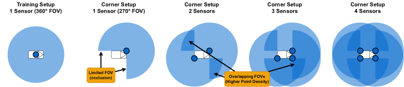
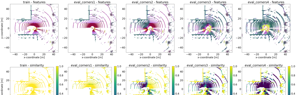
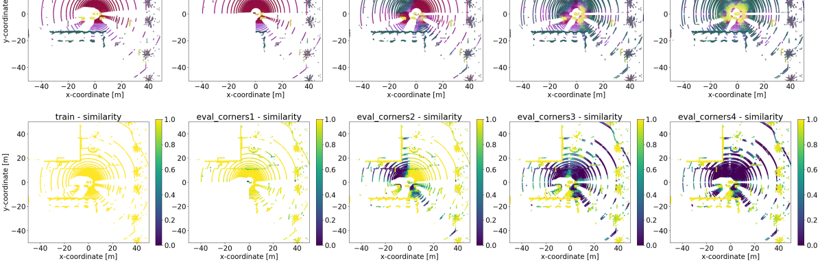
Figure 1: (a): A top-down illustration of the different LiDAR setups we simulate in our evaluation. The small blue circles indicate sensor positions on the roof of the vehicle. Multi-sensor setups often include overlapping Field-Of-Views from multiple sensors, or occlusions leading to blind spots with no coverage. (b): Point-wise feature visualization for point clouds from the sensor setups shown in (a), produced by 3-component PCA, mapped to RGB color values. (c): Normalized feature similarity between point features from the given setup and their nearest neighbor in the setup used for training.

3.1 Simulating Changes in Sensor Setups

Inspired by Fang et al. (2024), we generate simulated data for semantic segmentation using different sensor setups in the same environment, to isolate and investigate the effects of sensor setup changes to model performance. First, we simulate a setup similar to the nuScenes and SemanticKITTI datasets for training. This sensor setup consists of a single LiDAR sensor with 64 evenly spaced channels and 1024 points per channel, mounted centrally on the roof of the vehicle. Further details are provided in Appendix B.
We then train a sparse point-voxel CNN (Tang et al., 2020) on the data from this sensor setup (see Appendix D for details). After training the model, we evaluate it on a held-out test split to get a baseline in-domain generalization performance, as measured by the mIoU score, a commonly used metric for semantic segmentation performance (explained in Appendix C). In addition to our simulated data generated with the sensor setup, which we will further refer to as the training setup. We also generate data from the same simulation with different sensor setups (shown in Figure 1). In this way, we can isolate changes in sensor setup from other sources of domain shift, such as different environments or driving scenarios. We then evaluate the zero-shot generalization performance of our model on the test split of the new sensor setups. Additionally, since our simulations capture the same environment, we can compare the feature representations of the same environment across different sensor setups, which allows us to empirically quantify the invariance of our models.

3.2 Quantifying Invariance across Sensor Setups

In this section, we introduce a metric called normalized feature similarity to quantify the amount of invariance as the similarity between feature vectors from two corresponding data points related by a transformation. Then, we explain how we can employ it on non-aligned pairs of point clouds from different sensor setups.

Normalized Feature Similarity (NFS)

While performance metrics such as mIoU can empirically measure, whether a model generalizes to a different sensor setup, it does not provide any indication on whether the features used to obtain the final classification were the same, or if different features lead to the same final segmentation score. Therefore, inspired by Kvinge et al. (2022), we compare the feature vectors $\mathbf{f}$ of points across different sensor setups. Given two aligned sets of points $X\in\mathds{R}^{N\times 3},\,X=\{x_{i}\in\mathds{R}^{3}\mid i\in 1..N\}$ and $X^{\prime}\in\mathds{R}^{N\times 3},\,X^{\prime}=g(X)$ related by a transformation $g:\mathds{R}^{N\times 3}\to\mathds{R}^{N\times 3}$, along with features $F\in\mathds{R}^{N\times d},\,F=f(X)=\{\mathbf{f}_{i}\in\mathds{R}^{d}\mid i\in 1..N\}$ and $F^{\prime}=f(X^{\prime})=\{\mathbf{f^{\prime}}_{i}\in\mathds{R}^{d}\mid i\in 1..N\}$ computed by a feature extraction function $f$, we can compute the cosine similarity between the features of each point:

$$\mathrm{sim}(\mathbf{f}_{i},\,\mathbf{f^{\prime}}_{i})=\frac{\langle\mathbf{f}_{i},\,\mathbf{f^{\prime}}_{i}\rangle}{||\mathbf{f}_{i}||_{2}\,||\mathbf{f^{\prime}}_{i}||_{2}}$$

where $\langle\cdot,\cdot\rangle$ is the scalar product. Since the features extracted by neural networks can be arbitrarily shifted and scaled, we compute feature-wise mean $\boldsymbol{\mu}_{F}\in\mathds{R}^{d}$ and standard deviation $\boldsymbol{\sigma}_{F}\in\mathds{R}^{d}$ across the features $F$ to normalize the distribution of each feature and remove model-to-model variations in feature scales and shifts. Therefore, our normalized feature similarity (NFS) is computed as:

$$\mathrm{NFS}(F,F^{\prime})=\frac{1}{N}\sum_{i=1}^{N}sim\Bigg{(}\frac{\mathbf{f}_{i}-\boldsymbol{\mu}_{F}}{\boldsymbol{\sigma}_{F}},\,\frac{\mathbf{f^{\prime}}_{i}-\boldsymbol{\mu}_{F}}{\boldsymbol{\sigma}_{F}}\Bigg{)}$$

Comparing Point Cloud Features from Different Sensor Setups

Naturally, the data transformation given by a change in sensor setup does not trivially permit a one-to-one mapping of LiDAR points from one setup to another, since different sensor setups do not necessarily sample the same locations of the environment. However, since we are able to perform deterministic simulations of the same environment with different simulated LiDAR setups, we can compare the features of points in close-by locations. Since locally close-by environment locations likely have similar semantic meaning, their feature representations should be approximately the same, as long as the distance between related points is small. In Figure 1, we can see that this is at least partially the case, as the feature representation of objects of the same class is mostly very similar, and does not vary much across close-by locations. In practice, we use a KD-Tree to perform a nearest-neighbor search around each point $x^{\prime}$ from the new sensor setup, and search for a matching point $x$ in the corresponding point cloud from the training setup. On this aligned data, we can use our normalized feature similarity to empirically quantify the amount of invariance our feature extraction exhibits under the chosen sensor setup change. For a better understanding of where changes in sensor data impact the model predictions, we can also omit the averaging across the aligned point clouds, and directly compute the normalized feature similarity for individual points in the transformed sensor point cloud. The resulting feature similarity for each point is visualized in Figure 1.

4 Augmentations for Invariance to Sensor Setup Changes

In this section, we describe our intuition for designing the augmentations proposed in this work, based on our understanding of lacking invariance described in Section 3, and detail the two augmentations we design to alleviate the lack of generalization seen in our model on multi-sensor setups.

4.1 Frustum Drop Augmentation

Based on observations from Figure 1, we suspect that our model is impacted by changes in Field of View. Therefore, we design an augmentation, which drops points from a randomly selected view frustum from the point cloud. This is the inverse of frustum culling, an operation commonly used in 3D game engines. Given a point cloud $X\in\mathds{R}^{N\times 3}=\{\mathbf{x}_{i}\in\mathds{R}^{3}~{}|~{}i\in 1..N\}$, our augmentation is performed as follows: We first sample a random origin coordinate $\mathbf{t}\in\mathds{R}^{3},\,\mathbf{t}\sim[-r,r]^{3}$ as the origin of the frustum from a uniform distribution, where r determines the size of the cube being sampled from. We use a value of 3 meters for $r$. Then, we select one of the points $\mathbf{x}_{j}$ from the point cloud $X$ at random as the center of the omitted frustum. We then compute azimuth angles $\theta_{i}$ and corresponding elevation angles $\psi_{i}$ for each point relative to the frustum origin, using the following equations:

$$\theta_{i}=\mathrm{atan2}\bigg{(}\frac{y}{x}\bigg{)} \psi_{i}=\mathrm{atan2}\bigg{(}\frac{z}{\sqrt{x^{2}+y^{2}}}\bigg{)} \begin{pmatrix}x\\ y\\ z\\ \end{pmatrix}=(\mathbf{x}_{i}-\mathbf{t})$$

Using our sampled point $\mathbf{x}_{j}$ as the center of the frustum, we compute relative angles $\Delta\theta_{i}=\arccos(\cos(\theta_{i}-\theta_{j}))$ and $\Delta\psi_{i}=\arccos(\cos(\psi_{i}-\psi_{j}))$. The combination of $\arccos$ and $\cos$ normalizes the angle difference to a positive value in the range of [0, 180°]. Finally, we drop all points $\mathbf{x}_{i}$ whose relative angles $\Delta\theta_{i}$ and $\Delta\psi_{i}$ are both within a range $[0,\Delta\theta_{\mathrm{max}}]$ and $[0,\Delta\psi_{\mathrm{max}}]$ respectively, where we sample $\Delta\theta_{\mathrm{max}}$ and $\Delta\psi_{\mathrm{max}}$ uniformly from the range [2.5°, 90°]. A new combination of parameters ($\mathbf{t}$, $j$, $\Delta\theta_{\mathrm{max}}$, and $\Delta\psi_{\mathrm{max}}$) is sampled randomly for each new point cloud. In effect, this augmentation removes at least one point, and up to half the field of view from the point cloud in a pyramid cone shape. This augmentation can also be thought of as a variation of CutOut augmentation (DeVries, 2017) on a spherical projection of the point cloud onto an arbitrary origin point.

4.2 Mis-Calibration Augmentation

Based on the understanding gained from Figure 1 that our model’s features differ strongly when scan patterns from two or more sensors overlap, we propose to artificially introduce such overlapping scan pattern artifacts in our training data. Since our aim is to augment training data from a single sensor setup, we cannot produce the exact effect of overlapping scan patterns. Based on the hypothesis that a change in point density is the main part of our data transformation which causes our drop in performance, we can simply duplicate our point cloud to create a point cloud with twice the local point density everywhere.
By applying a slight random rotation and translation to one of the copies, we can create an effect which looks similar to a mis-calibrated pair of sensors with the same scan pattern. More formally, we compute the copied point cloud $X^{\prime}$ as:

$$X^{\prime} =(X\cdot R^{\top})+\mathbf{t}^{\top} R=R_{z}(\alpha_{z})R_{y}(\alpha_{y})R_{x}(\alpha_{x})$$

$$\mathbf{t} \sim[-s_{xy},s_{xy}]^{2}\times[-s_{z},s_{z}] \alpha_{x},\alpha_{y},\alpha_{z}\sim[-\alpha_{\mathrm{max}},\alpha_{\mathrm{max}}]$$

where $R_{z}(\alpha)$ denotes a rotation around the z-axis with angle $\alpha$. We visualize the intuition behind this augmentation in Figure 2. As seen in this figure, our augmentation typically generates points which are slightly offset from the surface originally sampled by the LiDAR sensor. Therefore, we attempt to limit the offset caused by our augmentation to values that we assume to be similar to sensor noise.

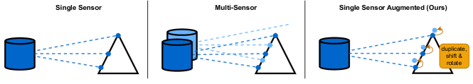
Figure 2: Multiple sensor instances scan the surface of objects with higher point density than a single sensor (compare left vs center). Additionally, they produce overlaps of different, non-aligned scan patterns. Our proposed mis-calibration augmentation (right) duplicates points from a single sensor, and applies a slight random shift and rotation to the duplicated pointcloud in order to replicate these aspects of a multi-sensor setup.

Therefore, we set $s_{xy}$, $s_{z}$ and $\alpha_{\mathrm{max}}$ to small values of 0.05 m and 0.05° respectively. We also experiment with a higher value of 1 m for $s_{xy}$, and find a surprisingly small negative impact on in-domain performance from this change. Since this augmentation causes an increase in the point density seen during batch training, we only apply it with a probability of up to 50% during training, as we reason that higher probabilities may cause our model to lose performance on the original training setup.

5 Results

In this section, we evaluate the effects of our two proposed augmentations on our model’s generalization to different sensor setups which the models have not seen during training.

[] []

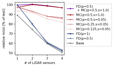
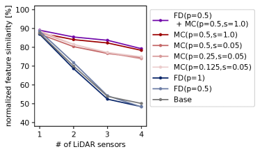
Figure 3: Comparing the effects of our augmentations on (a) relative mIoU score and (b) normalized feature similarity on the test partition of the unseen corner sensor setups shown in Figure 1. Notation is otherwise identical to Table 1.

	Train Setup	Corner Setups (zero-shot)
Augmentation	(Test Set)	1 Sensor	2 Sensors	3 Sensors	4 Sensors
Base	76.1	67.8	56.6	45.4	38.4
Base + FD(p=0.5)	75.8	75.9	60.3	46.4	40.3
Base + FD(p=1)	75.8	75.5	60.7	45.8	39.5
Base + MC(p=0.125, s=0.05)	77.6	72.5	71.5	66.4	63.6
Base + MC(p=0.25, s=0.05)	75.3	73.6	70.3	66.2	64.3
Base + MC(p=0.5, s=0.05)	76.3	74.4	70.9	67.2	66.0
Base + MC(p=0.5, s=1.0)	74.9	72.9	75.0	73.9	72.5
Base + FD(p=0.5) + MC(p=0.5, s=1.0)	74.9	74.5	75.3	74.1	72.5

Table 1: Generalization performance (mIoU Score $\uparrow$) of different augmentation configurations on the unseen test split of the sensor setups shown in Figure 1. Each row indicates a single model, trained on the training split of the train sensor setup. Base denotes our baseline set of augmentations as described in Section 3.1. MC(p, s) indicates adding our Mis-Calibration augmentation with probability p and shift magnitude s in meters ($s_{xy}$ in Section 4.2). FD(p) denotes our Frustum Drop augmentation with probability p.

5.1 Generalization to Multi-Sensor Setups

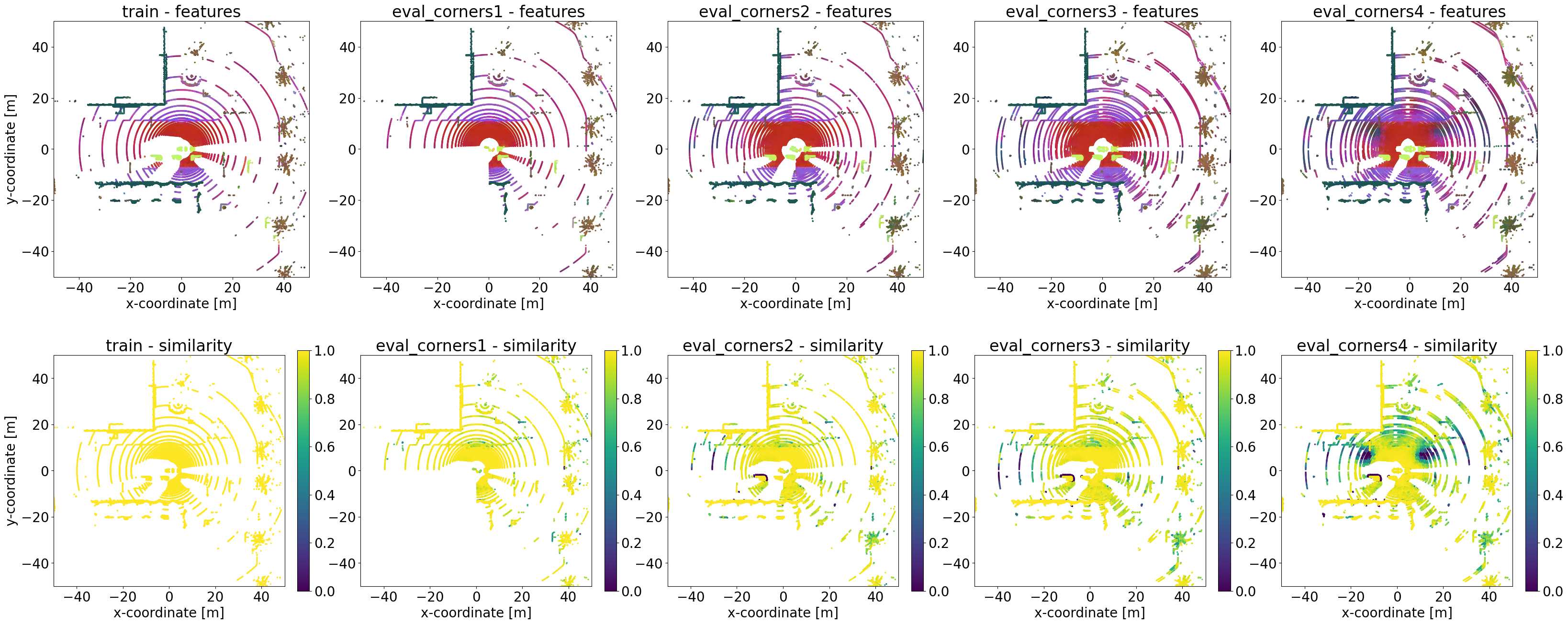
Figure 6: Model features (top) and normalized feature similarity (bottom) for the sensor setups from Figure 1, obtained from a model trained with both of our proposed augmentations. We observe much higher feature similarity (i.e. invariance) across the different sensor setups when compared to our baseline model without our proposed augmentations, which is shown in Figure 1 and 1

We first evaluate the performance impact of transferring trained models to the multi-sensor corner setups shown in Figure 1. We report mIoU scores for different augmentation configurations in Table 1, where each row corresponds to one trained model, which is evaluated on the test set of the different sensor setups. To eliminate differences in training setup performance, we plot the relative mIoU score (as a percentage of the mIoU on the training setup) in Figure 3. Our baseline set of augmentations (gray line) shows a steep and steady decline as the sensor setup is changed and more sensors are added, dropping from 76.1% mIoU to 67.8% mIoU on the single-sensor corner setup, down to 38.4% mIoU on four sensors, which is only half of the in-domain performance.
Our introduced Frustum Drop augmentation (blue lines in Figure 3) alleviates the noticeable differences between the training setup and the single-sensor corner setup, which indicates that the lower performance of the baseline model is likely caused by field-of-view changes. When using more sensors, the improvement of this augmentation quickly becomes negligible, and these models mirror the decline of the baseline model. In contrast, our Mis-Calibration augmentation (red lines in Figure 3) mitigates most of the performance decline seen on the multi-sensor setups, and only provides less benefit for the single-sensor setup. Noticeably, stronger versions of this augmentation also correspond to a stronger robustness to sensor setup changes, reaching up to 72.5% mIoU on the 4-sensor setup.
This is a mere 3% drop compared to the in-domain test set. Combining the best parameterizations of our introduced augmentations (purple line) combines the benefits of both, showing very consistent performance of at least 72.5% mIoU across all five sensor setups, and almost entirely alleviating our generalization deficit to our tested multi-sensor setups. Corresponding to Figure 1 which shows the features of the baseline model, we show the feature similarity plot with both of our proposed augmentations in Figure 6 in Appendix G.

Invariance Behavior

To quantify the effects of our augmentations on feature-level invariance, we plot our normalized feature similarity metric between features extracted from the training setup and the evaluated corner setups (described in Section 3.2) in Figure 3. In correspondence with the decline in mIoU score of our baseline model (gray line) in Figure 3, a corresponding drop in feature similarity across the different setups is seen in Figure 3. Similarly, we observe that our Mis-Calibration augmentation (red lines) appears to increase feature-level invariance roughly corresponding to the resulting mIoU score uplift. If our metric for feature-level invariance has predictive value for the resulting segmentation quality, this would be a very useful property, as the feature similarity can be computed on unlabeled data. However, while our Frustum Drop augmentation (blue lines) increases the mIoU score for the 1-sensor and 2-sensor corner setups, we do not observe a corresponding increase in feature-level invariance. Based on this different effect on invariance behavior, we suspect that two different mechanisms for improving generalization might be underlying our two augmentations. Further study is required to better understand these mechanisms.

5.2 Varying the Vertical Sensor Resolution

Since our augmentations work well to mitigate the performance impact of transitioning to our multi-sensor setups, we experiment with the effect of varying the resolution of the LiDAR sensor in our training setup. The number of channels, i.e. vertical resolution, is a common difference between commercially available LiDAR sensors of different price points, and affects the density of the point cloud in a similar way to adding more sensors. We also briefly experiment with varying the field of view of our sensor in Appendix F.
In Figure 4, we show the relative mIoU score on varying numbers of LiDAR channels, with Figure 4 showing the corresponding feature similarity. When deviating from the training setup (64 channels) in either direction, we observe a steep decline in mIoU score of the baseline model (gray line). At 16 channels, the mIoU score drops to 19.7% mIoU (-74% compared to train setup). When increasing the resolution to 256 channels the performance also drops to 39.7% mIoU (-48%).

[] []

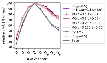
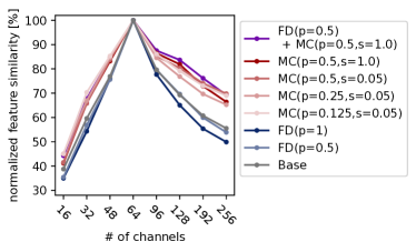
Figure 4: Comparing the effects of our augmentations on a) relative mIoU score and b) normalized feature similarity on variations of the training setup with varying vertical LiDAR resolution (# of channels). The training setup has 64 channels. mIoU scores are listed in Table 2 in Appendix E.

Our Frustum Drop augmentation (blue line) has a negligible effect on either metric in this experiment. Meanwhile, our Mis-Calibration augmentation significantly improves the mIoU score, especially when increasing the number of channels compared to the training setup. We, therefore, hypothesize that this augmentation improves invariance to point cloud density, which is supported by a roughly proportional increase in normalized feature similarity seen in Figure 4. Varying strengths of the augmentation only have a small effect in this experiment, with strong augmentations exhibiting slightly higher generalization and feature similarity. Combining both augmentations (purple line) has no detrimental effect, indicating that their mechanisms are, in a sense, orthogonal to each other.

6 Conclusion

In this work, we show that using the right data augmentation strategy can increase invariance across a select set of data transformations and thus improve out-of-domain generalization, using LiDAR semantic segmentation as an example. We introduce a new method to quantify feature-level invariance, which we call normalized feature similarity. Based on feature-level differences caused by changes in sensor setup, we derive two augmentations to imitate effects on the sensor data which directly affect the model’s features. Our experiments show that our augmentations mitigate a majority of the performance penalty incurred when training on a single-LiDAR setup and evaluating on our examined multi-sensor setups. We observe two mechanisms in which this may occur: one of our proposed augmentations seems to directly induce a feature-level invariance, while the other only improves our model’s performance on the shifted data distribution.

Limitations

In this work, we only explore a small and select set of LiDAR setups, and only provide results on simulated data. Additionally, generalization and invariance properties likely also depend on the used model architecture. We focus on a representative voxel-based CNN architecture in this work. Additional experiments are required to find out how our findings generalize to other architectures such as range image projections, or transformer-based approaches.

Future Work

We intend to explore the effects of different model architectures on the observed invariance properties in future work. Enforcing invariance through loss functions based on our proposed normalized feature similarity is also a promising avenue for future work. Finally, future work may uncover the mechanisms of why only some augmentations increase feature-level invariance, while others only have an effect on empirical performance.

Appendix A Background and Terminology on LiDAR Sensors

In this section, we provide a high-level overview of the working principle of LiDAR sensors, and introduce the resulting terminology.
LiDAR Sensors scan their environment by emitting short pulses of light in narrow beams which can be approximated as line-like rays. These rays reflect from objects in their surroundings, and part of the emitted light is reflected back to the sensor. By precisely measuring the round-trip time between emission and reflection, and multiplying by the speed of light, the sensor can detect the distance to the object which caused the reflection. By knowing the azimuth and elevation angle of the beam, and the resulting distance (often referred to as ”range”), a 3D coordinate (i.e. a ”point”) in sensor coordinates can be computed. By repeating this process across a large amount of different azimuth and elevation angles, these sensors can produce point clouds, consisting of a large number (approximately $10^{5}$) of 3D points in a short time span. This general principle is shared among most LiDAR sensors currently available, but sensors vary in their precision, maximum range, and – most relevant for this work – the pattern of azimuth and elevation angles which are sampled in each scan. In this work, we refer to the pattern of angle combinations probed in each scan as the ”scan pattern” or ”sampling pattern”. Due to rotating mechanical components, most LiDAR scanners emit their beams in evenly spaced horizontal rows, each typically sharing a single elevation angle across all of its points, while sampling azimuth angles in evenly spaced steps across the sensor’s horizontal field of view. These rows or lines are commonly named ”channels”, but also sometimes referred to as ”layers” in other literature, but we refrain from using the term ”layers” for this purpose in this work to avoid confusion with neural network terminology. Assuming a typical grid-like scan pattern with uniform elevation angle spacing of channels, a LiDAR sensor’s scan pattern is characterized by the following numbers: The horizontal and vertical Field of View (i.e. minimum and maximum azimuth and elevation angles respectively), the number of channels, and the number of points per channel (proportional to the horizontal angular resolution). Typical values for LiDAR sensors used in autonomous driving research and robotics include LiDAR sensors with vertical resolutions of between 16 and 256 channels, typically as powers of two. Similarly, for rotating sensors with a 360° horizontal Field of View, LiDAR sensors typically emit between 512 and 2048 points per channel during each rotation, typically also in powers of two. For more details on the mechanical system employed in LiDAR sensors, Li and Ibanez-Guzman (2020) provide an overview of the different measurement principles of LiDAR sensors used for automotive applications, as well as common methods for processing LiDAR sensor data.

Appendix B Simulation Details

We define a standardized scenario spanning 5.56 hours of simulated time (10,000 sensor time steps at 0.5 Hz) of driving through procedurally generated traffic in CARLA (Dosovitskiy et al., 2017) using the map Town 10. We use this same simulated scenario for all of our evaluations. We temporally split our scenario into a test, validation, and training split of 2000, 2000, and 6000 point clouds respectively. All simulated sensors use an evenly spaced angular distribution of channels across their vertical field of view, and are mounted at a height of 1.7 meters above the ground. Our simulated sensors use a vertical field of view of $\pm$22.5 degrees around the horizontal plane, for a total of 45 degrees, and a horizontal field of view of 360° for the training setup, and 270° for the corner setups. Unless stated otherwise, our sensors use a vertical resolution of 64 channels and a horizontal resolution of 1024 points per channel. This configuration is based on the sensor from the SemanticKITTI dataset.

Appendix C Semantic Segmentation and Metrics used in this Work

Semantic Segmentation

Semantic segmentation is a task in which the aim is to classify each component (e.g. each pixel in an image, or each point in a point cloud) into one of a pre-defined set of classes. In contrast to image or point cloud classification, which assigns a class to the entire data point, semantic segmentation provides more fine-grained spatial separation of object classes by assigning a semantic class to much smaller components of a data point. Therefore, it more suited for processing data which contains entire scenes with multiple objects at once, such as environment perception for autonomous vehicles.
Other related tasks for LiDAR point clouds include instance segmentation, where each point is classified as either part of a foreground object, or as part of the background, and foreground points are grouped into object instances. The combination of semantic segmentation and instance segmentation, i.e. assigning a semantic class to each point, and grouping points of foreground classes into instances, is called panoptic segmentation (Kirillov et al., 2019).
Another common task for autonomous driving perception is object detection, where 3D bounding boxes, including position, extent, and orientation, are predicted for each object in an image or 3D point cloud (Zamanakos et al., 2021).
In this work, we focus on semantic segmentation, as we expect it to benefit most from invariance properties. Since the other related tasks require more geometric information to be present for the final model output, we suspect invariance to potentially be detrimental, and methods promoting equivariance to be more suitable for those tasks.

mean Intersection-over-Union (mIoU)

For (supervised) Semantic Segmentation, we use the mean Intersection-over-Union metric, which is commonly employed for LiDAR semantic segmentation (Behley et al., 2019). For a dataset with $N$ points with corresponding labels $Y=\{y_{i}\in\mathcal{C}\,|\,i\in 1..N\}$ and corresponding predictions $\hat{Y}=\{\hat{y}_{i}\in\mathcal{C}\,|\,i\in 1..N\}$ from a set of classes $\mathcal{C}$, the mean IoU metric can be formalized as:

$$\mathrm{mIoU}(y,\hat{y})=\frac{1}{|\mathcal{C}|}\sum_{c\in\mathcal{C}}\frac{\sum_{i=1}^{N}\mathds{1}((\hat{y_{i}}=c)\wedge(y_{i}=c))}{\sum_{i=1}^{N}\mathds{1}((\hat{y}_{i}=c)\vee(y_{i}=c))}$$

The Intersection-over-Union (IoU) metric for a single class $c$ counts the number of points for which both prediction $\hat{y}_{i}$ and label $y_{i}$ belong to class $c$ (intersection), and divides it by the number of points where either prediction or label have class $c$ (union). For multi-class segmentation, the IoU metric is averaged across all classes, resulting in the mean IoU score (abbreviated as mIoU).

relative mIoU

Since models have slight performance deviations resulting from both training variance and the impact of augmentations, they achieve slightly different performance on the held-out validation/test split of the LiDAR setup used for training. As we are more interested in relative performance across different LiDAR setups in this work, we visualize the mIoU of each model on the test set of the evaluated setup, divided by its test set mIoU on the LiDAR setup used for training. Therefore, a model’s relative mIoU on an evaluation setup indicates the percentage of the original test set mIoU score, that a model receives on the new test set with a different setup. For transparency, we also list the model’s mIoU on the test set of the training setup in the first column of Table 1, so that the performance differences can be inferred.

Appendix D Training Methodology

We train a 3D sparse point-voxel convolutional neural network as introduced by Tang et al. (2020) for 50 epochs on the train split of 6000 simulated point clouds from the training setup. Our model architecture performs sparse convolutions at voxel sizes of [0.05, 0.1, 0.2, 0.4, 0.8, 1.6] meters, with respective feature dimensions scaled down to [8, 16, 32, 64, 128, 192] channels respectively. We also eliminate the up-scaling decoder layers as proposed by Tang et al. (2020), in order to achieve a latency of approximately 100ms on SemanticKITTI using an RTX 2080ti GPU. We use a single-cycle cosine learning rate decay schedule from an initial learning rate of 0.0016 down to 0 at the end of training. We train our model using the Adam optimizer, without weight decay. Our baseline set of augmentations is designed to increase robustness to SE(3) transformations, and consists of uniformly random translation in the x, y, and z directions up to 10 meters, uniformly random rotations in the pitch and roll axis of up to 10 degrees, and 360 degrees around the yaw (z) axis. Additionally, we apply instance-wise random translations of up to 1.0 m / 1.0 m / 0.1 m (x / y / z), and yaw rotations of up to 30° around their center to all objects within the point cloud. The augmentations proposed in this paper are applied after the baseline augmentations, which remain unchanged for all models in this work. Our final model has 2.2M parameters and achieves an mIoU score of approximately 61% on the SemanticKITTI (Behley et al., 2019) validation set using the described methodology, which is in accordance with results reported by Tang et al. (2020).

Appendix E Extended Results Comparing Changes in the Number of LiDAR Channels

For this experiment, we vary the vertical resolution (i.e. number of channels) of our LiDAR sensor from the training setup, as this is a common difference between commercially available LiDAR sensors. As modern sensor hardware evolves, we expect to see higher numbers of channels on future vehicles, which also makes invariance to increases in sensor resolution a desirable property. Since the vertical resolution often has a significant impact on the price of the sensor hardware, it is desirable that models still perform well with lower resolutions. Although we did not expect a significant performance difference on sensor resolutions lower than the 64 channels used in our training setup, we still incorporate them into this experiment for completeness. In our simulation, we keep the sensor position and field of view identical between all simulated sensor variations, and vary the number of channels from 64 in our training setup down to 16 and up to 256.

	# of Channels (Train Setup = 64)
Augmentation	16	32	48	64	96	128	192	256
Base	19.7	46.6	65.2	76.1	68.6	57.4	45.6	39.7
Base + FD(p=0.5)	20.6	48.8	65.7	75.8	68.5	56.2	46.3	42.0
Base + FD(p=1)	20.4	45.5	64.6	75.8	67.9	56.2	45.4	39.2
Base + MisCal(p=0.125,s=0.05)	31.0	54.1	69.9	77.6	74.1	69.3	59.6	55.2
Base + MisCal(p=0.25,s=0.05)	31.0	54.9	70.6	75.3	73.7	68.0	59.6	55.3
Base + MisCal(p=0.5,s=0.05)	30.5	55.7	70.9	76.3	74.1	69.2	62.4	58.5
Base + MisCal(p=0.5,s=1.0)	26.3	55.5	68.7	74.9	73.7	70.2	61.1	52.7
Base + FD(p=0.5) + MisCal(p=0.5,s=1.0)	29.1	55.6	68.7	74.9	73.5	70.1	63.0	54.2

Table 2: Generalization performance (mIoU Score $\uparrow$) of different augmentation configurations on the unseen test split, using variations of the training sensor setup with different numbers of uniformly spaced channels. Each row indicates a single model, trained on the training split of the train sensor setup. Notation is otherwise identical to Table 1.

Appendix F Evaluating Changes in Sensor Field of View

For this experiment, we simulate a reduced horizontal Field-of-View, with a proportionally lower number of points per channel, resulting in approximately the same azimuth angle spacing of LiDAR rays from the sensor.

[] []

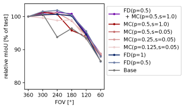
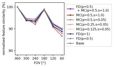
Figure 5: Comparing the effects of different horizontal Field of View on a) relative mIoU score and b) normalized feature similarity.

We observe in Figure 5 that changes in Field of View generally have a less noticeable impact on the semantic segmentation performance compared to the other two changes examined in Section 5. Our proposed Frustum Drop augmentation appears to alleviate performance drops in the range covered by the occlusion parameters, which is occlusions with angular extents of up to 180°, equating to FOV ranges from 360 to 180°. Outside this range, we observe a more noticeable, and very similar drop in performance across all our evaluated models. We declare the effects of adding our Mis-Calibration augmentation as inconclusive for this sensor setup change. Adding our augmentation appears to slightly increase robustness. However, when taking the generally small changes in mIoU into account, we do not have as high confidence in the statistical significance of these results. When re-running two training runs with identical augmentation configurations, we observe a run-to-run standard deviation in mIoU scores of approximately 0.6 mIoU points, with a peak difference of up to 2.5 mIoU points between runs.
In Figure 5, we observe that the normalized feature similarity is approximately equivalent for all of our models in this experiment. Similar to Section 5.1, we again observe no noticeable difference in feature-level invariance caused by our Frustum Drop augmentation, but in this case, the Mis-Calibration augmentation also appears to have no effect in this regard. The slight increase in relative mIoU scores observed in Figure 5 could therefore either be a result of invariance learned in the final classification layer, or be an artifact of run-to-run variance. We also see slight artifacts caused by rounding the horizontal sensor resolution to integer values. Since our default number of points per channel, 1024 (a typical value among LiDAR sensors) across 360°, is not evenly divisible by 60° increments, slight rounding deviations occur in multiple cases. This is indicated by the high feature similarity at 180°, which does not exhibit these rounding errors.

Appendix G Feature Similarity Plot with Augmentation

References

- Ayala and Mohd (2021) Rodrigo Ayala and Tauheed Khan Mohd. Sensors in autonomous vehicles: A survey. Journal of Autonomous Vehicles and Systems, 1(3):031003, 2021.
- Behley et al. (2019) Jens Behley, Martin Garbade, Andres Milioto, Jan Quenzel, Sven Behnke, Cyrill Stachniss, and Jurgen Gall. Semantickitti: A dataset for semantic scene understanding of lidar sequences. In Proceedings of the IEEE/CVF international conference on computer vision, pages 9297–9307, 2019.
- Botev et al. (2022) Aleksander Botev, Matthias Bauer, and Soham De. Regularising for invariance to data augmentation improves supervised learning. arXiv preprint arXiv:2203.03304, 2022.
- Bouchacourt et al. (2021) Diane Bouchacourt, Mark Ibrahim, and Ari Morcos. Grounding inductive biases in natural images: invariance stems from variations in data. Advances in Neural Information Processing Systems, 34:19566–19579, 2021.
- Caesar et al. (2020) Holger Caesar, Varun Bankiti, Alex H Lang, Sourabh Vora, Venice Erin Liong, Qiang Xu, Anush Krishnan, Yu Pan, Giancarlo Baldan, and Oscar Beijbom. nuscenes: A multimodal dataset for autonomous driving. In Proceedings of the IEEE/CVF conference on computer vision and pattern recognition, pages 11621–11631, 2020.
- Chen et al. (2021) Haiwei Chen, Shichen Liu, Weikai Chen, Hao Li, and Randall Hill. Equivariant point network for 3d point cloud analysis. In Proceedings of the IEEE/CVF conference on computer vision and pattern recognition, pages 14514–14523, 2021.
- Cohen and Welling (2016) Taco Cohen and Max Welling. Group equivariant convolutional networks. In International conference on machine learning, pages 2990–2999. PMLR, 2016.
- DeVries (2017) Terrance DeVries. Improved regularization of convolutional neural networks with cutout. arXiv preprint arXiv:1708.04552, 2017.
- Dosovitskiy et al. (2017) Alexey Dosovitskiy, German Ros, Felipe Codevilla, Antonio Lopez, and Vladlen Koltun. Carla: An open urban driving simulator. In Conference on robot learning, pages 1–16. PMLR, 2017.
- Fang et al. (2024) Jin Fang, Dingfu Zhou, Jingjing Zhao, Chenming Wu, Chulin Tang, Cheng-Zhong Xu, and Liangjun Zhang. Lidar-cs dataset: Lidar point cloud dataset with cross-sensors for 3d object detection. In 2024 IEEE International Conference on Robotics and Automation (ICRA), pages 14822–14829. IEEE, 2024.
- Heinrich et al. (2024) Marc Heinrich, Maximilian Zipfl, Marc Uecker, Sven Ochs, Martin Gontscharow, Tobias Fleck, Jens Doll, Philip Schörner, Christian Hubschneider, Marc René Zofka, et al. Cocar nextgen: a multi-purpose platform for connected autonomous driving research. arXiv preprint arXiv:2404.17550, 2024.
- Karle et al. (2023) Phillip Karle, Tobias Betz, Marcin Bosk, Felix Fent, Nils Gehrke, Maximilian Geisslinger, Luis Gressenbuch, Philipp Hafemann, Sebastian Huber, Maximilian Hübner, et al. Edgar: An autonomous driving research platform–from feature development to real-world application. arXiv preprint arXiv:2309.15492, 2023.
- Kim and Park (2019) Tae-Hyeong Kim and Tae-Hyoung Park. Placement optimization of multiple lidar sensors for autonomous vehicles. IEEE Transactions on Intelligent Transportation Systems, 21(5):2139–2145, 2019.
- Kimura et al. (2024) Masanari Kimura, Ryotaro Shimizu, Yuki Hirakawa, Ryosuke Goto, and Yuki Saito. On permutation-invariant neural networks. arXiv preprint arXiv:2403.17410, 2024.
- Kirillov et al. (2019) Alexander Kirillov, Kaiming He, Ross Girshick, Carsten Rother, and Piotr Dollár. Panoptic segmentation. In Proceedings of the IEEE/CVF conference on computer vision and pattern recognition, pages 9404–9413, 2019.
- Kvinge et al. (2022) Henry Kvinge, Tegan Emerson, Grayson Jorgenson, Scott Vasquez, Tim Doster, and Jesse Lew. In what ways are deep neural networks invariant and how should we measure this? Advances in Neural Information Processing Systems, 35:32816–32829, 2022.
- Li and Ibanez-Guzman (2020) You Li and Javier Ibanez-Guzman. Lidar for autonomous driving: The principles, challenges, and trends for automotive lidar and perception systems. IEEE Signal Processing Magazine, 37(4):50–61, 2020.
- Liu et al. (2019) Zhijian Liu, Haotian Tang, Yujun Lin, and Song Han. Point-voxel cnn for efficient 3d deep learning. Advances in neural information processing systems, 32, 2019.
- Qi et al. (2017) Charles R Qi, Hao Su, Kaichun Mo, and Leonidas J Guibas. Pointnet: Deep learning on point sets for 3d classification and segmentation. In Proceedings of the IEEE conference on computer vision and pattern recognition, pages 652–660, 2017.
- Tang et al. (2020) Haotian Tang, Zhijian Liu, Shengyu Zhao, Yujun Lin, Ji Lin, Hanrui Wang, and Song Han. Searching efficient 3d architectures with sparse point-voxel convolution. In European conference on computer vision, pages 685–702. Springer, 2020.
- Weiler et al. (2018) Maurice Weiler, Fred A Hamprecht, and Martin Storath. Learning steerable filters for rotation equivariant cnns. In Proceedings of the IEEE Conference on Computer Vision and Pattern Recognition, pages 849–858, 2018.
- Zaheer et al. (2017) Manzil Zaheer, Satwik Kottur, Siamak Ravanbakhsh, Barnabas Poczos, Russ R Salakhutdinov, and Alexander J Smola. Deep sets. Advances in neural information processing systems, 30, 2017.
- Zamanakos et al. (2021) Georgios Zamanakos, Lazaros Tsochatzidis, Angelos Amanatiadis, and Ioannis Pratikakis. A comprehensive survey of lidar-based 3d object detection methods with deep learning for autonomous driving. Computers & Graphics, 99:153–181, 2021.
- Zhao et al. (2021) Hengshuang Zhao, Li Jiang, Jiaya Jia, Philip HS Torr, and Vladlen Koltun. Point transformer. In Proceedings of the IEEE/CVF international conference on computer vision, pages 16259–16268, 2021.
- Zhu et al. (2021) Xinge Zhu, Hui Zhou, Tai Wang, Fangzhou Hong, Yuexin Ma, Wei Li, Hongsheng Li, and Dahua Lin. Cylindrical and asymmetrical 3d convolution networks for lidar segmentation. In Proceedings of the IEEE/CVF conference on computer vision and pattern recognition, pages 9939–9948, 2021.