Self-sustained patchy turbulence in shear-thinning active fluids

Abstract

Bacterial suspensions and other active fluids can develop highly dynamical vortex states called mesoscale turbulence. Here, we reveal the pronounced effect of non-Newtonian rheology of the carrier fluid, concentrating on shear thinning. Remarkably, this leads to hysteretic emergence of the turbulent state as a function of activity. A self-sustained heterogeneous state of coexisting turbulent and quiescent areas is identified. We find the signature of a directed percolation transition. Our results are important, for instance, when addressing active objects in biological media.

Bacterial suspensions are a paradigmatic example of active matter [1, 2, 3, 4]. Due to the constant energy input on the scale of the microswimmers, such suspensions exhibit various kinds of spatiotemporal patterns [5]. These include biofilm formation [6] as well as collective motion and swarming states [7, 8], which enable the rapid expansion to new territories. In particular, swimming bacteria display swirling and vortex patterns of characteristic length scale in terms of the vortex size [9, 10, 11]. This highly dynamic state has been denoted as active or mesoscale turbulence [11, 12]. The key features are captured by continuum-theoretical descriptions [11, 13, 14], which can be derived from generic microscopic models [15].

Both the propulsion mechanism and the interactions between microswimmers are mediated by the solvent medium. In general, the environments which bacteria and other biological microswimmers live in often display non-Newtonian and viscoelastic properties [16]. Examples include spermatozoa in the reproductive tract [17] and pathogenic bacteria in gastric mucus or other extracellular fluids [18]. Predominantly, blood shows shear thinning and can display complex rheological properties such as viscoelasticity and thixotropy [19]. During biofilm formation, bacteria excrete extracellular polymeric substances [6, 20], likewise resulting in non-Newtonian rheology [21].

The development of realistic models for collective motion of microswimmers thus necessitates to include non-Newtonian effects. So far, complex solvents have mostly been investigated in the case of single-swimmer dynamics, for instance, exploring the impact of viscoelasticity and shear thinning or thickening on the swimming speed [22, 23, 24]. These studies show that, depending on various parameters such as swimmer geometry and fluid properties, complex rheology can enhance or hinder self-propulsion [25, 26]. It allows for reciprocal deformations of the swimmers to achieve propulsion [27, 28, 29, 30], in contrast to Newtonian fluids featuring time-reversible Stokes flow [31, 32].

So far, only a limited number of studies explore the impact of complex rheological properties on the collective motion of microswimmers. Here, the focus has generally been on viscoelastic fluids. Diverse spatiotemporal pattern formation is observed, which results in enhanced complexity or calming effects depending on the elastic parameters [33, 34, 35, 36, 37, 38]. Recent studies have further demonstrated that complex rheological properties such as shear thickening [39] and viscoelasticity [40] can be utilized to control emergent states. However, in experiments bacterial suspensions often display shear thinning due to the presence of extracellular polymers [21]. The impact of these rheological conditions on active turbulence are still to be explored.

We address this open question through a recent continuum theory [14, 41, 42] that successfully describes experimental observations on both bacterial microswimmers and ATP-driven microtubular networks. Its versatility, besides characterizing pure active turbulence, has been demonstrated, for example, by extensions for shear-thickening active suspensions [39]. We now provide the missing and significantly more abundant case of mesoscale turbulence in shear-thinning suspensions. That is, viscosity locally decreases with increasing local shear rate. We explore the resulting patterns of turbulence and find, as a key observation, that shear thinning leads to anomalous velocity statistics and hysteretic behavior of the turbulent state when varying the activity. Remarkably, a regime of coexisting patterns of turbulence and macroscopically quiescent patches (vanishing collective velocity) emerges through shear thinning. Thus, we uncover a self-sustained dynamic state of heterogeneity combining regions of turbulence with nonturbulent patches.

Model equations

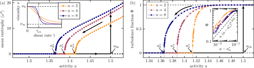
Figure 1: Hysteresis loops for the degree of mesoscale turbulence as a function of microswimmer activity $a$ for shear thinning parameters $\nu_{0}/\nu_{\infty}=1.5$, $\zeta=2$ and different $n$. For increasing $a$, the isotropic, macroscopically quiescent state becomes linearly unstable beyond $a_{\mathrm{th}}$. When decreasing $a$, turbulence persists down to the critical values $a^{*}_{n}<a_{\mathrm{th}}$. (a) Quantification via the system-averaged enstrophy $\langle\omega^{2}\rangle$. Inset: considered effect of shear thinning as described by the dependence of the local viscosity $\nu$ on the local shear rate $\dot{\gamma}$ [43, 44]. (b) Quantification via the time-averaged area fraction of turbulent patches $\Phi$. Inset: $\Phi$ as function of the distance to the critical value, $a-a_{n}^{\ast}$, revealing a regime of power-law scaling.

In the employed framework [14, 41, 42, 39], the dynamics of the overall (collective) velocity field $\mathbf{v}(\mathbf{x},t)$ of the entire suspension is described by a generalized, incompressible Navier–Stokes equation,

$$\partial_{t}\mathbf{v}+\mathbf{v}\cdot\nabla\mathbf{v}=-\nabla\tilde{p}+\nabla\cdot\tilde{\boldsymbol{\sigma}}\,,\qquad\nabla\cdot\mathbf{v}=0\,.$$ (1)

Here, the constant density $\rho$ is absorbed into the pressure and stress tensor, $\tilde{p}=p/\rho$ and $\tilde{\boldsymbol{\sigma}}=\boldsymbol{\sigma}/\rho$. Following Refs. 14, 41, 42, 39, the stress tensor is expanded in gradients of the deformation rate tensor $\boldsymbol{\Sigma}=[(\nabla\mathbf{v})+(\nabla\mathbf{v})^{\top}]/2$,

$$\tilde{\boldsymbol{\sigma}}=(\Gamma_{0}+\Gamma_{2}\nabla^{2}+\Gamma_{4}\nabla^{4})\big{[}(\nabla\mathbf{v})+(\nabla\mathbf{v})^{\top}\big{]}\,,$$ (2)

where ^⊤ marks the transpose. Key features are the emergence of highly dynamic vortex patterns and the selection of a specific length scale of the vortex size.

For $\Gamma_{2}=\Gamma_{4}=0$, the theory reduces to the familiar situation of vanishing activity. Then, $\Gamma_{0}$ corresponds to the kinematic viscosity ${\nu}$. We adopt the relation $\Gamma_{0}={\nu}$ for the active case. The coefficient $\Gamma_{4}$ must be positive to ensure stability at short wavelengths. The activity of the swimmers increases the coefficient $\Gamma_{2}$, which excites patterns of intermediate wavelengths once $\Gamma_{2}>\sqrt{4{\nu}\Gamma_{4}}$. A linear stability analysis reveals a critical finite wavenumber $k_{\mathrm{c}}=\sqrt{\Gamma_{2}/2\Gamma_{4}}$. The resulting band of unstable modes indicates wavenumbers at which energy is pumped into the system as a result of the intrinsic activity of the microswimmers. Subsequently, nonlinear advection, represented by $\mathbf{v}\cdot\nabla\mathbf{v}$ in Eq. (1), is responsible for the development of turbulence and associated energy transport between wavenumbers. The resulting balance between energy input and dissipation leads to a statistically stationary state [14, 41, 42, 39].

To investigate how the interplay of non-Newtonian rheology and active energy input impacts the emerging patterns, we now turn to the abundant case of shear-thinning active suspensions. The dependence of the local viscosity ${\nu}(\mathbf{x})$ on the local shear rate $\dot{\gamma}(\mathbf{x})$ is described in terms of the frequently considered Cross fluid [43, 44]. Its main feature is a viscosity ${\nu}_{\infty}$ at high shear rate that is smaller than the viscosity ${\nu}_{0}$ at low shear rate, accompanied by a continuous crossover region in between,

$${\nu}(\mathbf{x})={\nu}_{\infty}+\frac{{\nu}_{0}-{\nu}_{\infty}}{1+[\dot{\gamma}(\mathbf{x})/{\dot{\gamma}_{\mathrm{cr}}}]^{n}}\,.$$ (3)

The local shear rate is calculated from the deformation rate tensor via $\dot{\gamma}(\mathbf{x})=\sqrt{2\boldsymbol{\Sigma}(\mathbf{x}):\boldsymbol{\Sigma}(\mathbf{x})}$. While the exponent $n$ quantifies the steepness of the crossover, the reference shear rate $\dot{\gamma}_{\mathrm{cr}}$ locates this crossover, see the inset of Fig. 1(a).

We utilize the length $k_{\mathrm{c}}^{-1}$, the time $(k_{\mathrm{c}}^{2}{\nu}_{\infty})^{-1}$, and the speed $k_{\mathrm{c}}{\nu}_{\infty}$ to rescale Eq. (1),

$$\partial_{t}\mathbf{v}+\mathbf{v}\cdot\nabla\mathbf{v}=-\nabla\tilde{p}+\nabla\cdot(2\nu\boldsymbol{\Sigma}/\nu_{\infty})+a(2\nabla^{4}\mathbf{v}+\nabla^{6}\mathbf{v})\,,$$ (4)

where $\nu/\nu_{\infty}=1+(\nu_{0}/\nu_{\infty}-1)/\{1+[\sqrt{2\boldsymbol{\Sigma}:\boldsymbol{\Sigma}}/\zeta]^{n}\}$. The parameters characterizing shear thinning are the viscosity ratio $\nu_{0}/\nu_{\infty}$, the rescaled crossover shear rate $\zeta=\dot{\gamma}_{\mathrm{cr}}/(k_{\mathrm{c}}^{2}\nu_{\infty})$, and the exponent $n$. Moreover, $a=\Gamma_{2}^{2}/(4\nu_{\infty}\Gamma_{4})$ sets the strength of the activity of the microswimmers. Finally, $\mathbf{v}(\mathbf{x},t)$ quantifies the solvent flow on length scales several times larger than that of individual microswimmers. Thus, the isotropic state $\mathbf{v}(\mathbf{x},t)=\mathbf{0}$ describes macroscopic quiescence. It is characterized by the absence of collective motion, although the swimmers are active on the microscopic scale.

A straightforward linear stability analysis shows that the isotropic state $\mathbf{v}(\mathbf{x},t)=\mathbf{0}$ is stable below a threshold activity $a_{\mathrm{th}}=\nu_{0}/\nu_{\infty}$, see Appendix A for details. Increasing the activity above $a_{\mathrm{th}}$, this state becomes unstable with respect to the growth of patterns characterized by a band of unstable modes. The fastest-growing mode $k_{\mathrm{m}}$ is close to the critical mode $k_{\mathrm{c}}=1$ for values of $a$ close to $a_{\mathrm{th}}$. For $a=0$, we recover the familiar Navier–Stokes equation without activity for a shear-thinning Cross fluid.

Emerging heterogeneous patterns

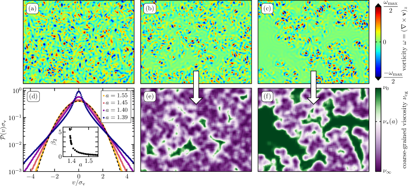
Figure 2: Coexistence of turbulent and macroscopically quiescent regions in the hysteretic regime. Snapshots of the vorticity field $\omega$ (rescaled by its respective maximum value $\omega_{\mathrm{max}}$) for activities (a) $a=1.55>a_{\mathrm{th}}$, (b) $a=1.41<a_{\mathrm{th}}$, and (c) $a=1.39$. Quiescent patches of increasing size develop for decreasing $a$. (d) Velocity distribution function $\mathcal{P}(v)$. Statistics are very close to Gaussian (indicated by the dashed line) for large activity $a$. Yet, they develop pronounced tails and an elevated maximum for decreasing $a$. Both axes are normalized using the standard deviation $\sigma_{v}$. Inset: excess kurtosis $\beta_{2}$ as a function of $a$, quantifying deviations from Gaussian statistics. (e,f) Snapshots of the locally averaged, coarse-grained viscosity $\nu_{\mathrm{cg}}(\mathbf{x})$ for the same values of $a$ as in (b,c). Remaining parameters are $\nu_{0}/\nu_{\infty}=1.5$, $n=4$, $\zeta=2$, and the size of the snapshots is $32\pi\times 24\pi$.

To analyze the emerging patterns that result from this combination of mesoscale turbulence and shear thinning, we solve Eq. (4) numerically for a large two-dimensional system of size $128\pi\times 128\pi$ with periodic boundary conditions. We start from random initial conditions and set the parameters to $\zeta=2$ and $\nu_{0}/\nu_{\infty}=1.5$, while varying the activity $a$. For details on the numerical methods, we refer to Appendix B. We begin below the threshold, $a<a_{\rm{th}}$, and then increase the activity $a$. Turbulence develops across the whole system once the threshold $a_{\mathrm{th}}$ is passed, where the quiescent state becomes linearly unstable, see the vertical black arrows in Fig. 1(a). There, the degree of mesoscale turbulence is quantified by the mean enstrophy $\langle\omega^{2}\rangle$, where we define the vorticity field $\omega=(\nabla\times\mathbf{v})_{z}$.

The case of decreasing activity $a$ features even more interesting behavior. We start above the threshold, $a>a_{\textrm{th}}$, implying that the macroscopically quiescent state is linearly unstable. Thus, vortex patterns grow across the whole system according to the finite-wavelength instability discussed above. For illustration, Fig. 2(a) shows a snapshot of the vorticity field at $a=1.55>a_{\textrm{th}}$. Remarkably, when now decreasing the activity $a$, turbulence persists down to below the threshold value $a_{\mathrm{th}}$, at which the macroscopically quiescent state becomes linearly unstable. We have not observed such hysteretic behavior for regular Newtonian fluids. The associated hysteresis loops of mesoscale turbulence, quantified by the mean enstrophy $\langle\omega^{2}\rangle$, are plotted in Fig. 1(a) for different values of $n$. To explain this hysteretic behavior, that is, the persistence of existing turbulence under decreasing activity $a<a_{\mathrm{th}}$, we note the following. In the existing turbulent state, relatively high local shear rates are present. Locally, due to shear thinning, these high shear rates significantly reduce viscosity. Reduced viscosity, in turn, favors turbulence. It thus provides a channel for self-sustenance of existing turbulence.

Decreasing activity further, we observe increasingly heterogeneous states, see the snapshots in Fig. 2(b) and (c). Compared to Fig. 2(a), the system now exhibits turbulent regions coexisting with increasingly large quiescent areas devoid of vortices. This emergent heterogeneous state is highly dynamic and the locations of the macroscopically quiescent patches continuously change while the vortex patterns rearrange. Remarkably, the development of heterogeneous states of coexistence also fundamentally changes the velocity statistics $\mathcal{P}(v)$. Here, $v$ represents an arbitrary component of the velocity field, $v=v_{x}$ or $v=v_{y}$. Due to macroscopic isotropy, either component can be used. In previous studies, employing a similar statistical evaluation [11, 45, 46, 47] for the Newtonian case, the velocity statistics were found to be very close to Gaussian. We observe the same behavior in the fully turbulent state for $a>a_{\mathrm{th}}$, see Fig. 2(d). However, when decreasing activity in our situation of shear thinning below the threshold value $a_{\mathrm{th}}$, the distribution function develops pronounced tails together with a sharper maximum at $v=0$. These features reflect heterogeneous states of coexisting macroscopically quiescent areas ($v\approx 0$) and turbulent regions of elevated local macroscopic velocities.

Since already the turbulent regions themselves are very heterogeneous, we employ a coarse-graining procedure, see Appendix C, to further quantify the emerging structures. Across the system, we locally average the viscosity over square regions of a size corresponding to the critical length scale $2\pi k_{c}^{-1}$. Snapshots of the resulting coarse-grained viscosity field $\nu_{\mathrm{cg}}(\mathbf{x})$ are depicted in Fig. 2(e) and (f). To distinguish between turbulent and macroscopically quiescent regions, we introduce a color scheme. If the locally coarse-grained viscosity is large enough to suppress the linear instability and thus turbulence, $\nu_{\mathrm{cg}}(\mathbf{x})>\nu_{\ast}(a)=a\,\nu_{\infty}$, we employ green color. Contrarily, low-viscosity regions of locally self-sustained turbulence are dyed in purple. In particular, Fig. 2(e) and (f) demonstrates the coexistence of turbulent and macroscopically quiescent regions of comparable area fraction.

Universality of the transition to turbulence

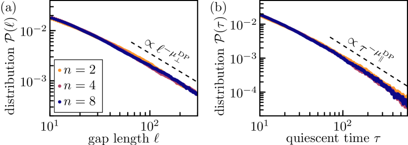
Figure 3: Features of the spatial and temporal structures near the critical point in terms of the distributions $\mathcal{P}$ of (a) the distances (lengths of the gaps) between the turbulent regions $\ell$ and (b) the time intervals of local quiescence $\tau$, for $n=2$ ($a=1.41460$), $n=4$ ($a=1.38825$), and $n=8$ ($a=1.36585$). Remaining parameters are $\nu_{0}/\nu_{\infty}=1.5$ and $\zeta=2$. The emergent power-law scaling near the transition for elevated $\ell$ and $\tau$ is consistent with $2+1$ directed percolation (“DP”), as indicated by the dashed lines, according to the exponents $\mu_{\perp}^{\mathrm{DP}}=1.204(2)$ and $\mu_{\parallel}^{\mathrm{DP}}=1.5495(10)$ [48, 49]

To further quantify the transition from fully developed turbulence to macroscopically quiescent states, we determine the time-averaged area fraction of turbulence $\Phi$ via the coarse-grained viscosity. We define the fluid at position $\mathbf{x}$ as turbulent if $\nu_{\mathrm{cg}}(\mathbf{x})<\nu_{*}(a)=a\,\nu_{\infty}$. $\Phi$ acts as an order parameter. Its bounds indicate a macroscopically quiescent state of the entire system ($\Phi=0$) and fully turbulent ones ($\Phi=1$). Figure 1(b) shows $\Phi$ as a function of activity $a$ for different values of $n$. For decreasing $a$, we observe a clear transition from a fully turbulent to a completely quiescent state. Here, the critical value $a_{n}^{\ast}$ is shifted to smaller activities for larger $n$, thus extending the region of hysteresis and coexistence. Remarkably, when we plot $\Phi$ as a function of the distance to the critical point $(a-a_{n}^{\ast})$, see the inset of Fig. 1(b), we observe power-law behavior $\Phi\propto(a-a_{n}^{\ast})^{\beta^{\ast}}$ with $\beta^{\ast}=0.352(20)$. Additional simulations presented in Appendix D demonstrate that the exponent $\beta^{\ast}$ depends on the rescaled crossover shear rate $\zeta$.

Power-law scaling indicates that the transition may be linked to a universality class of non-equilibrium phase transitions. Indeed, recent studies [48, 50, 51, 52, 53] have shown that emergence of turbulence in various systems can be understood as a transition of directed percolation. Thus, we focus on the behavior near the critical point. We determine the distances (lengths of the gaps) between turbulent regions $\ell$ and their distribution $\mathcal{P}(\ell)$. Moreover, we measure local intervals of quiescent times $\tau$ and their distribution $\mathcal{P}(\tau)$. See Appendix E for more details on these quantities and calculations. As for directed percolation [49], the spatial and temporal structures exhibit self-similarity near the critical point. There, the distributions $\mathcal{P}(\ell)$ and $\mathcal{P}(\tau)$ show power-law scaling. Fig. 3 shows the distributions in our system at parameter values very close to the critical activity. The scaling and corresponding exponents are consistent with behavior in $2+1$ directed percolation (two space and one time dimension), see Appendix E for more details. The scaling of directed percolation (“DP”) is indicated in Fig. 3 by the dashed lines.

State diagram

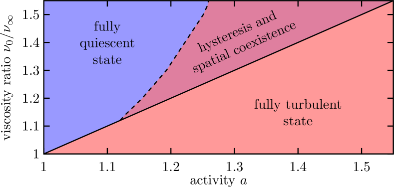
Figure 4: State diagram for the entire system as a function of activity $a$ and viscosity ratio $\nu_{0}/\nu_{\infty}$ for $\zeta=1$ and $n=4$. The quiescent state is linearly unstable for $a>\nu_{0}/\nu_{\infty}$ (diagonal line), resulting in a fully turbulent state. For activities below linear instability, $a<\nu_{0}/\nu_{\infty}$, but right to the dashed line, there is a region of hysteresis and spatial coexistence between turbulent and quiescent regions.

Finally, to summarize, Fig. 4 shows a state diagram of the shear-thinning active suspension as a function of activity $a$ and viscosity ratio $\nu_{0}/\nu_{\infty}$. The linear instability of the quiescent state for $a>\nu_{0}/\nu_{\infty}$ yields the diagonal line, right of which we always encounter a fully turbulent state of the entire system. Left of the diagonal, a hysteretic region of coexistence is found, if $a\gtrsim 1.12$ (see also Appendix D). Further to the left, we find the state of complete macroscopic quiescence. Here, for these low activities, local shear rates do not reach the low-viscosity regime and coexistence between turbulence and quiescence is thus ruled out.

Conclusions

Overall, we reveal that shear thinning leads to hysteresis of mesoscale turbulence as a function of activity, combined with heterogeneous spatial coexistence of self-sustained turbulent and macroscopically quiescent regions in active suspensions. Concerning the associated anomalous velocity statistics, we mention related experimental observations on bacterial suspensions of Bacillus Subtilis [54, 8]. There, motile and immotile areas coexist, for instance, due to the presence of sublethal doses of antibiotics [55] or elevated aspect ratios [8]. We here provide an illustrative explanation via non-Newtonian shear thinning. For instance, excretions of bacteria [6, 20, 21] can induce such shear thinning in biological suspensions. Our explanation is not based on density variations as involved, for example, in motility-induced phase separation [56, 57].

From a fundamental perspective, our study extends recent attempts of linking nonequilibrium transitions, such as the emergence of turbulence [50, 51, 53, 58], to universality classes of statistical physics, ranging from Ising behavior [59, 60] to directed percolation [48, 50, 51, 52, 53]. In the more practical context of applications, the observed phenomena are relevant for microfluidic and mesoscale mixing based on active suspensions [61, 62, 63, 64, 65, 66]. Mesoscale turbulence enhances mixing. We have demonstrated that, through shear thinning, the regime of mesoscale turbulence can be extended to lower activities, as the system becomes heterogeneous and maintains self-sustained turbulent patches. In a way, the situation reminds of type-II superconductors, where, in analogy, applications can be extended to higher magnetic fields, maintaining superconductivity through emergent spatial heterogeneities in the system [67].

Appendix A Linear stability analysis

In this appendix, we present the linear stability analysis for the rescaled Navier–Stokes equation, that is, Eq. (4) in the main text. In particular, we consider the stability of the macroscopically quiescent solution $\mathbf{v}_{0}=\mathbf{0}$.

As a first step, we add a small perturbation to velocity and pressure,

$$\mathbf{v}(\mathbf{x},t)=\mathbf{v}_{0}+\delta\mathbf{v}(\mathbf{x},t)\,,\quad\tilde{p}(\mathbf{x},t)=\tilde{p}_{0}+\delta\tilde{p}(\mathbf{x},t)\,.$$ (5)

To continue, we make the ansatz

$$\delta\mathbf{v}(\mathbf{x},t)=\delta\hat{\mathbf{v}}\,e^{\lambda t+i\mathbf{k}\cdot\mathbf{x}}\,,\quad\delta\tilde{p}(\mathbf{x},t)=\delta\hat{p}\,e^{\lambda t+i\mathbf{k}\cdot\mathbf{x}}\,,$$ (6)

where $\lambda$ is the complex growth rate and $\mathbf{k}$ is the wavevector of the perturbation. We insert Eqs. (5) and (6) into Eq. (4) of the main text and linearize around the quiescent solution. Evaluating the temporal and spatial derivatives, we obtain

$$\lambda\delta\hat{\mathbf{v}}=-i\mathbf{k}\delta\hat{p}-\left(\nu_{0}|\mathbf{k}|^{2}/\nu_{\infty}-2a|\mathbf{k}|^{4}+a|\mathbf{k}|^{6}\right)\delta\hat{\mathbf{v}}\,.$$ (7)

Multiplying by $\mathbf{k}$ and using the incompressibility condition $\mathbf{k}\cdot\delta\hat{\mathbf{v}}=0$ implies that $\delta\hat{p}=0$. Thus, the growth rate $\lambda$ as a function of the wavevector is determined as

$$\lambda(\mathbf{k})=-\nu_{0}|\mathbf{k}|^{2}/\nu_{\infty}+2a|\mathbf{k}|^{4}-a|\mathbf{k}|^{6}\,.$$ (8)

We note that $\lambda(\mathbf{k})$ is always real and find that it can become positive for

$$a>a_{\mathrm{th}}=\nu_{0}/\nu_{\infty}.$$ (9)

This defines the threshold value $a_{\mathrm{th}}$ as introduced in the main text. There, a finite-wavelength instability sets in. Modes associated with the wavenumber $k_{\mathrm{c}}=1$ start to grow. Increasing $a$ above $a_{\mathrm{th}}$, a band of unstable modes develops. The wavenumber of the mode of maximum growth rate $k_{\mathrm{m}}$ is close to the critical wavenumber $k_{\mathrm{c}}$.

When investigating the spatial coexistence of turbulent and macroscopically quiescent domains, we apply the relations derived above for global stability to the local scale. Locally, the quantity of interest is the coarse-grained local viscosity $\nu_{\mathrm{cg}}(\mathbf{x},t)$, see main text and Appendix. C below. We rearrange the stability condition Eq. (9) for the quiescent state and replace $\nu_{0}$ by $\nu_{\mathrm{cg}}(\mathbf{x},t)$. Then, we expect, approximately, a quiescent domain to be stable if, for that domain, $\nu_{\mathrm{cg}}(\mathbf{x},t)>\nu^{\ast}(a)=a\nu_{\infty}$. Contrarily, if $\nu_{\mathrm{cg}}(\mathbf{x},t)<\nu^{\ast}=a\nu_{\infty}$, local perturbations grow and turbulence can sustain itself in this area. Overall, this condition allows to distinguish between turbulent and quiescent domains. It forms the basis of the color scale that we have chosen for illustration in Fig. 2(e) and (f) of the main text. Green color indicates quiescent domains of $\nu_{\mathrm{cg}}(\mathbf{x},t)>\nu^{\ast}$, whereas purple color marks turbulent regions of $\nu_{\mathrm{cg}}(\mathbf{x},t)<\nu^{\ast}$.

Appendix B Numerical methods

We employ a pseudo-spectral method to solve Eq. (4) of the main text in a two-dimensional system with periodic boundary conditions. Time integration is performed via a fourth-order Runge-Kutta method. It is combined with an operator splitting technique treating the linear and nonlinear parts consecutively [68]. To enforce the incompressibility condition $\nabla\cdot\mathbf{v}=0$, the pressure $\tilde{p}$ is effectively treated as a Lagrange multiplier used to ensure that the velocity field $\mathbf{v}(\mathbf{x},t)$ stays divergence-free.

The main results are obtained by starting the numerical calculations for an activity $a$ that is large enough for turbulence to develop. That is, we select $a>\nu_{0}/\nu_{\infty}$, implying that the macroscopically quiescent state is linearly unstable. The initial conditions are set to $\mathbf{v}(\mathbf{x},t)=\mathbf{0}$, with small random perturbations added to each velocity component at every grid point, following a uniform distribution over $[-0.01,0.01]$. We then decrease the activity $a$ in small steps, let the calculations run for $500$ time units, and store the resulting velocity fields for subsequent calculations. These fields are used as initializations for further long-time calculations. Before analyzing the dynamics, we always let the simulations for a set of parameters run for at least $10000$ time units to ensure the development of statistically stationary states. Close to the critical point, simulations are run even longer (up to $30000$ time units). The mean enstrophy $\langle\omega^{2}\rangle$, the velocity distribution $\mathcal{P}(v)$, the turbulence fraction $\Phi$, and the coarse-grained viscosity distribution $\mathcal{P}(\nu_{\mathrm{cg}}/\nu_{\infty})$, see below, are averaged over $5$ consecutive time intervals of $1500$ time units. Error bars in the figures denote the standard error, that is, the standard deviation divided by the square root of the number of time intervals. The velocity statistics $\mathcal{P}(v)$ as shown in Fig. 2(d) of the main text are determined as an average over $\mathcal{P}(v_{x})$ and $\mathcal{P}(v_{y})$, that is, the distributions for $x$ and $y$ velocity components, respectively. Due to the statistical dynamical isotropy of the turbulent state, the distributions are the same within our statistical errors, regardless of direction.

For most calculations, the system size is set to $128\pi\times 128\pi$ and the spatial resolution to $768\times 768$ grid points. To obtain the state diagram shown in Fig. 5 of the main text and Fig. 7, we rather use a system size of $64\pi\times 64\pi$ and $384\times 384$ grid points. These sizes are quite large compared to the vortex size, which is close to the critical length scale $2\pi/k_{\mathrm{c}}=2\pi$. We only explore activity regimes of $a<1.55$ [14].

Appendix C Coarse-graining procedure

To analyze the coexistence of turbulent and macroscopically quiescent regions in space, we first employ a coarse-graining procedure to smoothen the locally nonuniform vortex patterns. In particular, we average the local viscosity over a square region of side length $\Delta x$ around each point in space. The resulting coarse-grained viscosity field $\nu_{\mathrm{cg}}(\mathbf{x},t)$ at location $\mathbf{x}=(x,y)$ is thus obtained from the field $\nu(\mathbf{x},t)$ via

$$\nu_{\mathrm{cg}}(\mathbf{x},t)=\frac{1}{\Delta x^{2}}\int_{y-\Delta x/2}^{y+\Delta x/2}\ \int_{x-\Delta x/2}^{x+\Delta x/2}\nu(\tilde{\mathbf{x}},t)\,\mathrm{d}\tilde{x}\,\mathrm{d}\tilde{y}\,,$$ (10)

where $\tilde{\mathbf{x}}=(\tilde{x},\tilde{y})$. As the vortex structures emerge from the finite-wavelength instability at $a=\nu_{0}/\nu_{\infty}$, we here choose a side length $\Delta x$ equal to the critical length scale, that is, $\Delta x=2\pi/k_{\mathrm{c}}=2\pi$. The more refined structure of patterns is thus averaged out.

Snapshots of the coarse-grained viscosity $\nu_{\mathrm{cg}}(\mathbf{x},t)$ are included in Fig. 2 of the main text. As discussed there, they clearly show the presence of both low- and high-viscosity regions, corresponding to the turbulent and macroscopically quiescent state, respectively. To further illustrate our observations in the main text, we additionally determine the distribution $\mathcal{P}(\nu_{\mathrm{cg}}/\nu_{\infty})$. It quantifies how much of the system exhibits high or low viscosity. This distribution is plotted in Fig. 5 for two values of activity, $a=1.5$ and $a=1.41$. For the larger activity $a=1.5$, there is only one maximum in $\mathcal{P}(\nu_{\mathrm{cg}}/\nu_{\infty})$. It reflects the presence of a fully turbulent system. However, for the smaller activity $a=1.41$, we observe that a second maximum has emerged, here at $\nu_{\mathrm{cg}}/\nu_{\infty}=1.5$. It corresponds to the quiescent state. The presence of two maxima implies that there are separate, spatially coexisting regions of turbulence and of quiescence.

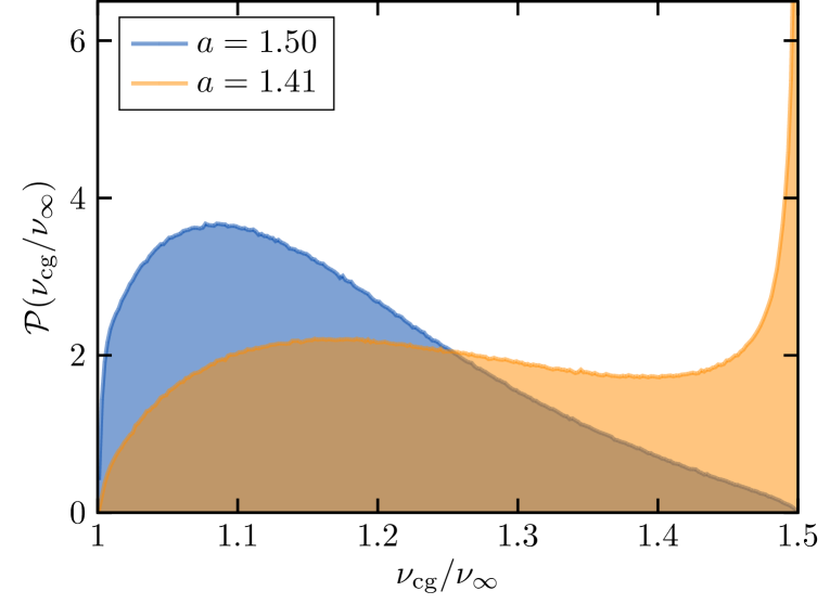
Figure 5: Distribution function $\mathcal{P}(\nu_{\mathrm{cg}}/\nu_{\infty})$ for the coarse-grained viscosity $\nu_{\mathrm{cg}}$ for two different example values of activity. For larger values, here $a=1.5$, we observe a single maximum. It reflects a fully turbulent state. For lower values, here $a=1.41$, two maxima are present, They point to spatially coexisting regions of low and high viscosity, corresponding to turbulence and to quiescence, respectively. The other parameters are set to $\nu_{0}/\nu_{\infty}=1.5$, $n=4$ and $\zeta=2$.

Appendix D Robustness of the results

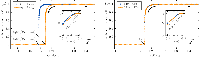
Figure 6: Time-averaged area fraction of turbulent domains $\Phi$ as a function of activity $a$ for crossover shear rate $\zeta=1$ and degree of sharpness of the crossover $n=4$ of shear thinning. (a) Decreasing the viscosity ratio $\nu_{0}/\nu_{\infty}$ shifts the critical value of activity $a_{4}^{\ast}$, the lower bound of hysteresis, to smaller values. Inset: Within the considered resolution, the power-law scaling close to the critical point is not affected by the change in $\nu_{0}/\nu_{\infty}$. Yet, it depends on the crossover shear rate $\zeta$, as a comparison with Fig. 3 in the main text shows. For $\zeta=1$ we find a power-law scaling $\Phi\propto(a-a_{4}^{\ast})^{\beta^{\ast}}$ with exponent $\beta^{\ast}=0.103(5)$, whereas for $\zeta=2$ (see Fig. 3 in the main text), we find $\beta^{\ast}=0.342(20)$. (b) When changing the system sizes as indicated for $\nu_{0}/\nu_{\infty}=1.4$, we do not observe any significant change in the area fraction of turbulent regions as a function of activity $a$.

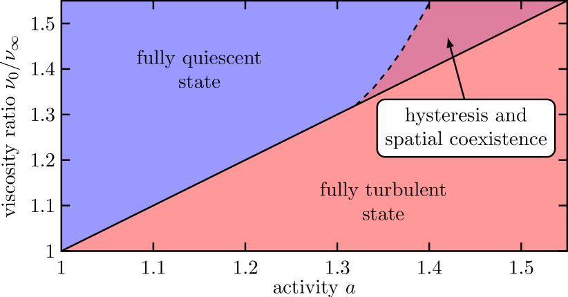
Figure 7: State diagram as a function of activity $a$ and viscosity ratio $\nu_{0}/\nu_{\infty}$ for crossover shear rate $\zeta=2$ and steepness of the crossover $n=4$ of shear thinning. The quiescent state is linearly unstable with respect to turbulence at activities above $a>\nu_{0}/\nu_{\infty}$ (diagonal line), resulting in a fully turbulent state. For activities $a$ left to the diagonal but above a certain value $a\gtrsim 1.32$, there is a region of hysteresis and spatial coexistence between turbulent and quiescent domains. At lower activities $a\lesssim 1.32$, we always find complete macroscopic quiescence.

In the main text, we mainly discuss our results on one set of example values, namely for the crossover shear rate of $\zeta=2$ and the viscosity ratio of $\nu_{0}/\nu_{\infty}=1.5$. Yet, as indicated, these results are rather general. To illustrate the robustness, we here include additional data when varying the parameter values and system size.

Figure 6(a) shows the turbulence fraction $\Phi$ as a function of activity $a$ for $\zeta=1$, steepness of the crossover of shear thinning set by $n=4$, and two different viscosity ratios, $\nu_{0}/\nu_{\infty}=1.3$ and $\nu_{0}/\nu_{\infty}=1.4$. As in Fig. 3 in the main text, we observe a continuous decrease of the area fraction of turbulent regions with decreasing activity $a$ until a critical point is reached at $a=a_{4}^{\ast}$. There, the whole system becomes macroscopically quiescent. Due to the lower crossover shear rate $\zeta=1$, when compared to $\zeta=2$ in Fig. 3, the critical activity $a_{4}^{\ast}$ is smaller.

We further observe that an increase in the viscosity ratio $\nu_{0}/\nu_{\infty}$ shifts the critical activity $a_{4}^{\ast}$ to higher values. The inset of Fig. 6 shows the scaling of $\Phi$ when approaching the critical activity from above. As in Fig. 3 in the main text, we again observe power-law scaling $\Phi\propto(a-a_{4}^{\ast})^{\beta^{\ast}}$, although the exponent $\beta^{\ast}$ is different. However, we did not observe $\beta^{\ast}$ to depend on the value of the viscosity ratio $\nu_{0}/\nu_{\infty}$.

Taken altogether, these results suggest that the exponent is independent or only weakly dependent on both $\nu_{0}/\nu_{\infty}$ and $n$, while it depends on the value of the crossover shear rate $\zeta$. For $\zeta=1$, we find an exponent $\beta^{\ast}=0.103(5)$, whereas for $\zeta=2$, we find $\beta^{\ast}=0.352(20)$. The exponents were determined from fits to the data points. Numbers in brackets denote error estimates corresponding to confidence intervals of $95\text{\,}\mathrm{\char 37\relax}$.

In order to check for finite-size effects, we plot the turbulence fraction $\Phi$ as a function of activity $a$ for different system sizes at $\zeta=1$, $n=4$, and $\nu_{0}/\nu_{\infty}=1.4$ in Fig. 6(b). Clearly, the data points for system sizes of $64\pi\times 64\pi$ and $128\pi\times 128\pi$ coincide, indicating the robustness of the results. In particular, the systems considered in our investigations are large enough so that finite-size effects do not play any obvious role for these data.

Finally, Fig. 7 shows the state diagram for $\zeta=2$ and $n=4$. When compared with Fig. 5 in the main text, we observe that an increase in crossover shear rate shifts the region of hysteresis and spatial coexistence to higher activity $a$. We find the following explanation. The turbulent and quiescent state correspond to low- and high-viscosity domains, respectively. Both regimes must be accessible for the system, so that these two states can coexist. However, for too low activity $a$, local shear rates mostly remain too low so that shear thinning does not set in effectively. Thus, the system does not reach the low-viscosity regime. In particular, local shear rates must significantly exceed the crossover shear rate $\zeta$ for shear thinning to play a significant role. Together with an increased value of $\zeta$, the minimum required activity $a$ to facilitate self-sustained turbulence based on shear thinning thus becomes larger. Consequently, the coexistence region in the state diagram is shifted to the right.

Appendix E Universality of the transition

$\quad\ \zeta\quad\$	$\ \ \nu_{0}/\nu_{\infty}\ \$	$\quad n\quad$	$\qquad\ a\qquad\$	$\qquad\ \mu_{\perp}\qquad\$	$\qquad\quad\mu_{\parallel}\qquad\quad$	regions used for parameter fits
$1$	$1.3$	$4$	1.19399	$1.207(14)$	$\quad 1.5258(40)$	$60<\ell<160$	$20<\tau<500$
$1$	$1.4$	$4$	1.22220	$1.251(5)$	$1.5678(37)$	$20<\ell<100$	$20<\tau<500$
$2$	$1.5$	$2$	1.41460	$1.200(6)$	$1.5424(96)$	$50<\ell<300$	$90<\tau<400$
$2$	$1.5$	$4$	1.38825	$1.196(4)$	$1.5596(76)$	$50<\ell<150$	$50<\tau<300$
$2$	$1.5$	$8$	1.36585	$1.211(8)$	$1.5443(51)$	$110<\ell<300$	$50<\tau<700$
$\mu_{\perp}^{\mathrm{DP}}$ and $\mu_{\parallel}^{\mathrm{DP}}$ for $2+1$ directed percolation				$1.204(2)$	$1.5495(10)$

Table 1: Critical exponents $\mu_{\perp}$ and $\mu_{\parallel}$ of the power-law scalings $\mathcal{P}(\ell)\propto\ell^{-\mu_{\perp}}$ and $\mathcal{P}(\tau)\propto\tau^{-\mu_{\parallel}}$ for different sets of parameter values very close to the critical point. $\mathcal{P}(\ell)$ and $\mathcal{P}(\tau)$ are the distributions of the spatial distance between turbulent patches (gap lengths) $\ell$ and of the local quiescent time intervals between the occurrences of turbulence $\tau$, respectively. Values for the exponents are obtained via fitting the scaling laws to the data points in the intervals listed in the table. The exponent $\mu_{\perp}$ refers to the spatial dimension, $\mu_{\parallel}$ to the direction of percolation, thus here to the temporal dimension. For comparison, the exponents $\mu_{\perp}^{\mathrm{DP}}$ and $\mu_{\parallel}^{\mathrm{DP}}$ for $2+1$ directed percolation [48, 49] are included as well. Error estimates correspond to $95\text{\,}\mathrm{\char 37\relax}$ confidence intervals.

The power-law scaling of the area fraction of turbulent domains $\Phi$ as a function of the distance $a-a^{\ast}_{n}$ from the critical point, see Fig. 3 in the main text and Fig. 6, motivates the investigation of the transition in the context of universality classes of phase transitions. We here provide supplemental information concerning our approach.

The nonequilibrium nature of active systems in combination with the two coexisting dynamic states suggests that we should not expect the transition to fall into one of the equilibrium universality classes. We rather conjecture that consistency with a statistical phase transition, such as a percolation transition [49], can be revealed. In fact, in the context of driven inertial turbulence, such a correspondence has recently been established. In Ref. 51, it was demonstrated for driven passive systems that the transition to turbulence in Couette flow follows a transition of directed percolation. In this analogy, turbulent domains spreading to neighboring regions correspond to the excited state, whereas laminar domains correspond to the absorbing state. Above a certain critical Reynolds number, the turbulent domains may persist in time, thus leading to a percolation transition. The direction of the spreading process of directed percolation therefore corresponds to the time dimension of the driven fluid flow. Determining certain critical exponents for the turbulence transition in Couette flow, the analogy to $1+1$ directed percolation (one space and one time dimension) can be established [51]. In addition to driven Couette flow of passive systems, directed percolation transitions have been found in channel flow [52], pipe flow [50], turbulent liquid crystals [48], as well as active nematics [53].

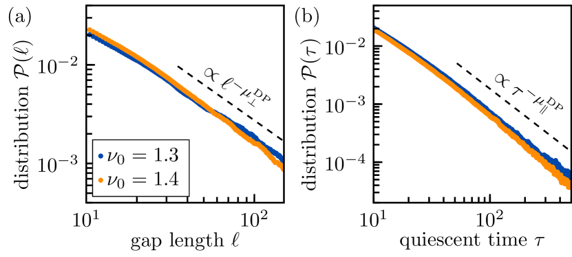
Figure 8: Features of the spatial and temporal structures near the critical point in terms of the distributions $\mathcal{P}$ of (a) the distances (lengths of the gaps) between the turbulent regions $\ell$ and (b) the time intervals of local quiescence $\tau$ for $\nu_{0}/\nu_{\infty}=1.3$ ($a=1.19399$) and $\nu_{0}/\nu_{\infty}=1.4$ ($a=1.22220$). Remaining parameters are $n=4$ and $\zeta=1$. The emergent power-law scaling near the transition for elevated $\ell$ and $\tau$ is consistent with $2+1$ directed percolation (“DP”), as indicated by the dashed lines, according to the exponents $\mu_{\perp}^{\mathrm{DP}}=1.204(2)$ and $\mu_{\parallel}^{\mathrm{DP}}=1.5495(10)$ [48, 49]

Motivated by these studies, we investigate whether our transition between a fully macroscopically quiescent system and patchy self-sustained turbulent states, as observed in our shear-thinning active fluid, likewise exhibits parallels with directed percolation. As shown in Fig. 3 of the main text and in Fig. 6, the area fraction of turbulent domains $\Phi$ scales according to a power law with the distance $a-a^{\ast}_{n}$ from the critical point. However, the power-law exponent depends on the magnitude of the crossover shear rate $\zeta$ of shear thinning. Directly comparing such exponents depending on the distance $a-a^{\ast}_{n}$ with those of the directed percolation universality classes thus seems futile. In fact, there is no a priori reason why the activity $a$ should linearly correspond to the spreading probability, which is the control parameter in directed percolation. Thus, we rather focus our attention on the critical point directly and not on how it is approached.

In directed percolation, the spatial and temporal correlations become scale-free at the critical point [49]. Accordingly and motivated by Refs. 51, 48, we thus focus on the distributions of certain characteristics of the absorbing state, which here is the quiescent state. Specifically, those characteristic parameters are the distances (gap lengths) between turbulent domains $\ell$ and the time intervals (duration) of quiescence between the occurrences of turbulence at fixed spatial positions $\tau$. The associated distributions $\mathcal{P}(\ell)$ and $\mathcal{P}(\tau)$ at the critical point scale according to power laws with their arguments. These power laws reflect self-similarity of the structures in both space and time.

Corresponding critical exponents here are defined via $\mathcal{P}(\ell)\propto\ell^{-\mu_{\perp}}$ and $\mathcal{P}(\tau)\propto\tau^{-\mu_{\parallel}}$. Generally, for $2+1$ directed percolation, the exponents are given by $\mu_{\perp}^{\mathrm{DP}}=1.204(2)$ and $\mu_{\parallel}^{\mathrm{DP}}=1.5495(10)$ [48]. In directed percolation, these exponents are related to the exponents of perpendicular (spatial) and parallel (temporal) correlation lengths, $\nu_{\perp}^{\mathrm{DP}}$ and $\nu_{\parallel}^{\mathrm{DP}}$, respectively, via $\mu_{\perp}^{\mathrm{DP}}=2-\beta^{\mathrm{DP}}/\nu_{\perp}^{\mathrm{DP}}$ and $\mu_{\parallel}^{\mathrm{DP}}=2-\beta^{\mathrm{DP}}/\nu_{\parallel}^{\mathrm{DP}}$ [48, 51]. There, $\beta^{\mathrm{DP}}$ is the critical exponent of the proportion of excited regions [48, 51].

To determine the distributions $\mathcal{P}(\ell)$ and $\mathcal{P}(\tau)$ at the critical point, we performed additional numerical calculations for the sets of parameters explored so far. We choose a value of the activity $a$ as close to the critical value $a_{n}^{\ast}$ as possible. The dynamics are analyzed in a window of $10000$ time units. We first determine distributions of gap lengths for the $x$ and $y$ directions separately. As the system exhibits isotropic symmetry in the statistical sense, these distributions, $\mathcal{P}(\ell_{x})$ and $\mathcal{P}(\ell_{y})$, are equal for large enough sample sizes. We thus calculate $\mathcal{P}(\ell)$ as the average of $\mathcal{P}(\ell_{x})$ and $\mathcal{P}(\ell_{y})$. The quiescent time distribution, $\mathcal{P}(\tau)$, can be determined directly. Results are summarized in Table 1, which includes the values for the fitted exponents $\mu_{\perp}$ and $\mu_{\parallel}$. Figure 4 in the main text shows the power-law scaling for a crossover shear rate of shear thinning $\zeta=2$, whereas the data for $\zeta=1$ are presented in Fig. 8. We observe power-law scaling of the distributions at sufficiently large $\ell$ and $\tau$ for all parameter sets.

In conclusion, the resulting exponents are consistent with the exponents of $2+1$ directed percolation $\mu_{\perp}^{\mathrm{DP}}$ and $\mu_{\parallel}^{\mathrm{DP}}$. Corresponding scaling is indicated by the dashed lines in the plots. It strongly indicates that the transition from patches of self-sustained turbulence to a homogeneous quiescent state spanning the whole system can indeed be understood as a transition of directed percolation.

References

- Marchetti et al. [2013] M. C. Marchetti, J. F. Joanny, S. Ramaswamy, T. B. Liverpool, J. Prost, M. Rao, and R. A. Simha, Hydrodynamics of soft active matter, Rev. Mod. Phys. 85, 1143 (2013).
- Bechinger et al. [2016] C. Bechinger, R. Di Leonardo, H. Löwen, C. Reichhardt, G. Volpe, and G. Volpe, Active particles in complex and crowded environments, Rev. Mod. Phys. 88, 045006 (2016).
- Bär et al. [2020] M. Bär, R. Großmann, S. Heidenreich, and F. Peruani, Self-propelled rods: Insights and perspectives for active matter, Annu. Rev. Condens. Matter Phys. 11, 441 (2020).
- Gompper et al. [2020] G. Gompper, R. G. Winkler, T. Speck, A. Solon, C. Nardini, F. Peruani, H. Löwen, R. Golestanian, U. B. Kaupp, L. Alvarez, et al., The 2020 motile active matter roadmap, J. Phys. Condens. Matter 32, 193001 (2020).
- Jeckel et al. [2019] H. Jeckel, E. Jelli, R. Hartmann, P. K. Singh, R. Mok, J. F. Totz, L. Vidakovic, B. Eckhardt, J. Dunkel, and K. Drescher, Learning the space-time phase diagram of bacterial swarm expansion, Proc. Natl. Acad. Sci. U.S.A. 116, 1489 (2019).
- Hall-Stoodley et al. [2004] L. Hall-Stoodley, J. W. Costerton, and P. Stoodley, Bacterial biofilms: From the natural environment to infectious diseases, Nat. Rev. Microbiol. 2, 95 (2004).
- Be’er and Ariel [2019] A. Be’er and G. Ariel, A statistical physics view of swarming bacteria, Mov. Ecol. 7, 1 (2019).
- Be’er et al. [2020] A. Be’er, B. Ilkanaiv, R. Gross, D. B. Kearns, S. Heidenreich, M. Bär, and G. Ariel, A phase diagram for bacterial swarming, Commun. Phys. 3, 66 (2020).
- Dombrowski et al. [2004] C. Dombrowski, L. Cisneros, S. Chatkaew, R. E. Goldstein, and J. O. Kessler, Self-concentration and large-scale coherence in bacterial dynamics, Phys. Rev. Lett. 93, 098103 (2004).
- Sokolov and Aranson [2012] A. Sokolov and I. S. Aranson, Physical properties of collective motion in suspensions of bacteria, Phys. Rev. Lett. 109, 248109 (2012).
- Wensink et al. [2012] H. H. Wensink, J. Dunkel, S. Heidenreich, K. Drescher, R. E. Goldstein, H. Löwen, and J. M. Yeomans, Meso-scale turbulence in living fluids, Proc. Natl. Acad. Sci. U.S.A. 109, 14308 (2012).
- Alert et al. [2022] R. Alert, J. Casademunt, and J.-F. Joanny, Active turbulence, Annu. Rev. Condens. Matter Phys. 13 (2022).
- Dunkel et al. [2013] J. Dunkel, S. Heidenreich, M. Bär, and R. E. Goldstein, Minimal continuum theories of structure formation in dense active fluids, New J. Phys. 15, 045016 (2013).
- Słomka and Dunkel [2015] J. Słomka and J. Dunkel, Generalized Navier–Stokes equations for active suspensions, Eur. Phys. J. Spec. Top. 224, 1349 (2015).
- Reinken et al. [2018] H. Reinken, S. H. L. Klapp, M. Bär, and S. Heidenreich, Derivation of a hydrodynamic theory for mesoscale dynamics in microswimmer suspensions, Phys. Rev. E 97, 022613 (2018).
- Li et al. [2021] G. Li, E. Lauga, and A. M. Ardekani, Microswimming in viscoelastic fluids, J. Non-Newt. Fluid Mech. 297, 104655 (2021).
- Fauci and Dillon [2006] L. J. Fauci and R. Dillon, Biofluidmechanics of reproduction, Annu. Rev. Fluid Mech. 38, 371 (2006).
- Celli et al. [2009] J. P. Celli, B. S. Turner, N. H. Afdhal, S. Keates, I. Ghiran, C. P. Kelly, R. H. Ewoldt, G. H. McKinley, P. So, S. Erramilli, et al., Helicobacter pylori moves through mucus by reducing mucin viscoelasticity, Proc. Natl. Acad. Sci. U.S.A. 106, 14321 (2009).
- Beris et al. [2021] A. N. Beris, J. S. Horner, S. Jariwala, M. J. Armstrong, and N. J. Wagner, Recent advances in blood rheology: A review, Soft Matter 17, 10591 (2021).
- Worlitzer et al. [2022] V. M. Worlitzer, A. Jose, I. Grinberg, M. Bär, S. Heidenreich, A. Eldar, G. Ariel, and A. Be’er, Biophysical aspects underlying the swarm to biofilm transition, Sci. Adv. 8, eabn8152 (2022).
- Jana et al. [2020] S. Jana, S. G. Charlton, L. E. Eland, J. G. Burgess, A. Wipat, T. P. Curtis, and J. Chen, Nonlinear rheological characteristics of single species bacterial biofilms, npj Biofilms Microbiomes 6, 19 (2020).
- Teran et al. [2010] J. Teran, L. Fauci, and M. Shelley, Viscoelastic fluid response can increase the speed and efficiency of a free swimmer, Phys. Rev. Lett. 104, 038101 (2010).
- Li and Ardekani [2015] G. Li and A. M. Ardekani, Undulatory swimming in non-Newtonian fluids, J. Fluid Mech. 784, R4 (2015).
- Datt et al. [2015] C. Datt, L. Zhu, G. J. Elfring, and O. S. Pak, Squirming through shear-thinning fluids, J. Fluid Mech. 784, R1 (2015).
- Montenegro-Johnson et al. [2013] T. D. Montenegro-Johnson, D. J. Smith, and D. Loghin, Physics of rheologically enhanced propulsion: Different strokes in generalized Stokes, Phys. Fluids 25 (2013).
- van Gogh et al. [2022] B. van Gogh, E. Demir, D. Palaniappan, and O. S. Pak, The effect of particle geometry on squirming through a shear-thinning fluid, J. Fluid Mech. 938, A3 (2022).
- Qiu et al. [2014] T. Qiu, T.-C. Lee, A. G. Mark, K. I. Morozov, R. Münster, O. Mierka, S. Turek, A. M. Leshansky, and P. Fischer, Swimming by reciprocal motion at low Reynolds number, Nat. Commun. 5, 5119 (2014).
- Datt et al. [2018] C. Datt, B. Nasouri, and G. J. Elfring, Two-sphere swimmers in viscoelastic fluids, Phys. Rev. Fluids 3, 123301 (2018).
- Yasuda et al. [2020] K. Yasuda, M. Kuroda, and S. Komura, Reciprocal microswimmers in a viscoelastic fluid, Phys. Fluids 32 (2020).
- Eberhard et al. [2023] M. Eberhard, A. Choudhary, and H. Stark, Why the reciprocal two-sphere swimmer moves in a viscoelastic environment, Phys. Fluids 35 (2023).
- Purcell [1977] E. M. Purcell, Life at low Reynolds number, Am. J. Phys. 45, 3 (1977).
- Lauga and Powers [2009] E. Lauga and T. R. Powers, The hydrodynamics of swimming microorganisms, Rep. Prog. Phys. 72, 096601 (2009).
- Bozorgi and Underhill [2013] Y. Bozorgi and P. T. Underhill, Role of linear viscoelasticity and rotational diffusivity on the collective behavior of active particles, J. Rheol. 57, 511 (2013).
- Bozorgi and Underhill [2014] Y. Bozorgi and P. T. Underhill, Effects of elasticity on the nonlinear collective dynamics of self-propelled particles, J. Non-Newt. Fluid Mech. 214, 69 (2014).
- Hemingway et al. [2015] E. J. Hemingway, A. Maitra, S. Banerjee, M. C. Marchetti, S. Ramaswamy, S. M. Fielding, and M. E. Cates, Active viscoelastic matter: From bacterial drag reduction to turbulent solids, Phys. Rev. Lett. 114, 098302 (2015).
- Hemingway et al. [2016] E. J. Hemingway, M. E. Cates, and S. M. Fielding, Viscoelastic and elastomeric active matter: Linear instability and nonlinear dynamics, Phys. Rev. E 93, 032702 (2016).
- Li and Ardekani [2016] G. Li and A. M. Ardekani, Collective motion of microorganisms in a viscoelastic fluid, Phys. Rev. Lett. 117, 118001 (2016).
- E. L. C. VI M. Plan et al. [2020] E. L. C. VI M. Plan, J. M. Yeomans, and A. Doostmohammadi, Active matter in a viscoelastic environment, Phys. Rev. Fluids 5, 023102 (2020).
- Reinken and Menzel [2024] H. Reinken and A. M. Menzel, Vortex pattern stabilization in thin films resulting from shear thickening of active suspensions, Phys. Rev. Lett. 132, 138301 (2024).
- Liu et al. [2021] S. Liu, S. Shankar, M. C. Marchetti, and Y. Wu, Viscoelastic control of spatiotemporal order in bacterial active matter, Nature 590, 80 (2021).
- Słomka and Dunkel [2017a] J. Słomka and J. Dunkel, Geometry-dependent viscosity reduction in sheared active fluids, Phys. Rev. Fluids 2, 043102 (2017a).
- Słomka and Dunkel [2017b] J. Słomka and J. Dunkel, Spontaneous mirror-symmetry breaking induces inverse energy cascade in 3d active fluids, Proc. Natl. Acad. Sci. U.S.A. 114, 2119 (2017b).
- Cross [1965] M. M. Cross, Rheology of non-newtonian fluids: A new flow equation for pseudoplastic systems, J. Colloid Sci. 20, 417 (1965).
- Barnes et al. [1989] H. A. Barnes, J. F. Hutton, and K. Walters, An introduction to rheology, Vol. 3 (Elsevier, Amsterdam, 1989).
- Bratanov et al. [2015] V. Bratanov, F. Jenko, and E. Frey, New class of turbulence in active fluids, Proc. Natl. Acad. Sci. U.S.A. 112, 15048 (2015).
- James and Wilczek [2018] M. James and M. Wilczek, Vortex dynamics and lagrangian statistics in a model for active turbulence, Eur. Phys. J. E 41, 21 (2018).
- Mukherjee et al. [2023] S. Mukherjee, R. K. Singh, M. James, and S. S. Ray, Intermittency, fluctuations and maximal chaos in an emergent universal state of active turbulence, Nat. Phys. 19, 891 (2023).
- Takeuchi et al. [2007] K. A. Takeuchi, M. Kuroda, H. Chaté, and M. Sano, Directed percolation criticality in turbulent liquid crystals, Phys. Rev. Lett. 99, 234503 (2007).
- Hinrichsen [2000] H. Hinrichsen, Non-equilibrium critical phenomena and phase transitions into absorbing states, Adv. Phys. 49, 815 (2000).
- Sipos and Goldenfeld [2011] M. Sipos and N. Goldenfeld, Directed percolation describes lifetime and growth of turbulent puffs and slugs, Phys. Rev. E 84, 035304(R) (2011).
- Lemoult et al. [2016] G. Lemoult, L. Shi, K. Avila, S. V. Jalikop, M. Avila, and B. Hof, Directed percolation phase transition to sustained turbulence in Couette flow, Nat. Phys. 12, 254 (2016).
- Sano and Tamai [2016] M. Sano and K. Tamai, A universal transition to turbulence in channel flow, Nat. Phys. 12, 249 (2016).
- Doostmohammadi et al. [2017] A. Doostmohammadi, T. N. Shendruk, K. Thijssen, and J. M. Yeomans, Onset of meso-scale turbulence in active nematics, Nat. Commun. 8, 15326 (2017).
- Ilkanaiv et al. [2017] B. Ilkanaiv, D. B. Kearns, G. Ariel, and A. Be’er, Effect of cell aspect ratio on swarming bacteria, Phys. Rev. Lett. 118, 158002 (2017).
- Benisty et al. [2015] S. Benisty, E. Ben-Jacob, G. Ariel, and A. Be’er, Antibiotic-induced anomalous statistics of collective bacterial swarming, Phys. Rev. Lett. 114, 018105 (2015).
- Worlitzer et al. [2021a] V. M. Worlitzer, G. Ariel, A. Be’er, H. Stark, M. Bär, and S. Heidenreich, Motility-induced clustering and meso-scale turbulence in active polar fluids, New J. Phys. 23, 033012 (2021a).
- Worlitzer et al. [2021b] V. M. Worlitzer, G. Ariel, A. Be’er, H. Stark, M. Bär, and S. Heidenreich, Turbulence-induced clustering in compressible active fluids, Soft Matter 17, 10447 (2021b).
- Reinken et al. [2024] H. Reinken, S. Heidenreich, M. Baer, and S. H. Klapp, Pattern selection and the route to turbulence in incompressible polar active fluids, New J. Phys. 26, 063026 (2024).
- Marcq et al. [1997] P. Marcq, H. Chaté, and P. Manneville, Universality in Ising-like phase transitions of lattices of coupled chaotic maps, Phys. Rev. E 55, 2606 (1997).
- Reinken et al. [2022a] H. Reinken, S. Heidenreich, M. Bär, and S. H. L. Klapp, Ising-like critical behavior of vortex lattices in an active fluid, Phys. Rev. Lett. 128, 048004 (2022a).
- Kim and Breuer [2004] M. J. Kim and K. S. Breuer, Enhanced diffusion due to motile bacteria, Phys. Fluids 16, L78 (2004).
- Sokolov et al. [2009] A. Sokolov, R. E. Goldstein, F. I. Feldchtein, and I. S. Aranson, Enhanced mixing and spatial instability in concentrated bacterial suspensions, Phys. Rev. E 80, 031903 (2009).
- Leptos et al. [2009] K. C. Leptos, J. S. Guasto, J. P. Gollub, A. I. Pesci, and R. E. Goldstein, Dynamics of enhanced tracer diffusion in suspensions of swimming eukaryotic microorganisms, Phys. Rev. Lett. 103, 198103 (2009).
- C. P. and Joy [2020] S. C. P. and A. Joy, Friction scaling laws for transport in active turbulence, Phys. Rev. Fluids 5, 024302 (2020).
- Mukherjee et al. [2021] S. Mukherjee, R. K. Singh, M. James, and S. S. Ray, Anomalous diffusion and Lévy walks distinguish active from inertial turbulence, Phys. Rev. Lett. 127, 118001 (2021).
- Reinken et al. [2022b] H. Reinken, S. H. L. Klapp, and M. Wilczek, Optimal turbulent transport in microswimmer suspensions, Phys. Rev. Fluids 7, 084501 (2022b).
- de Gennes [1999] P.-G. de Gennes, Superconductivity of metals and alloys (Westview Press, Boulder, 1999).
- Canuto et al. [2007] C. Canuto, M. Y. Hussaini, A. Quarteroni, and T. A. Zang, Spectral methods: Evolution to complex geometries and applications to fluid dynamics (Springer, Berlin Heidelberg, 2007).