Effective chiral response of anisotropic multilayered metamaterials

Abstract

We consider a multilayered metamaterial composed of anisotropic layers with in-plane anisotropy axes periodically rotated with respect to each other. Due to the breaking of inversion symmetry, the structure develops an effective chirality. We derive the effective chirality tensor of the metamaterial describing both normal and oblique incidence scenarios. We also identify the arrangement of the layers maximizing chiral response for the fixed lattice period, wavelength and anisotropy of the layers.

I Introduction

One of the most salient features of metamaterials is the emergence of effective properties beyond those of their constituent elements. While elementary building blocks of the structure are ordinary metals or dielectrics, their collective response to the electromagnetic excitation can be quite nontrivial. Besides celebrated negative effective permittivity and permeability [1, 2, 3], emergent properties include various forms of electromagnetic nonreciprocity [4, 5], nonlocality [6, 7] and even effective axion fields [8, 9].

One of such useful properties is chirality which is broadly defined as impossibility to superimpose object with its mirror image. Specifically, we focus on electromagnetic chirality that couples electric and magnetic responses of the medium, ensures different interaction of the medium with left- and right-hand circularly polarized waves [10, 11, 12] and originates due to the breaking of inversion symmetry. While different measures of chirality are discussed in the literature [13, 14, 15], here we introduce it as a tensor $\hat{\kappa}$ arising in the bulk material equations [16]

$$\begin{cases}\mathbf{D}=\hat{\varepsilon}\mathbf{E}+i\hat{\kappa}\mathbf{H},\\ \mathbf{B}=-i\hat{\kappa}^{\mathsf{T}}\mathbf{E}+\hat{\mu}\mathbf{H},\end{cases}$$ (1)

where $\hat{\varepsilon}$ and $\hat{\mu}$ are the conventional permittivity and permeability.

Chirality is ubiquitous in organic materials, where it stems from the non-centrosymmetric nature of the constituent molecules and can hardly be tuned. At the classical level, this physics is captured by the Born-Kuhn model [17]; quantum-mechanical description is also available [18].

At the same time, chirality can also be configurational arising due to the proper non-symmetric arrangement of centrosymmetric elements [19, 20]. This is the case for cholesteric liquid crystals utilized for LC displays technology [21, 22]. More recently, helical homostructures have been realized by stacking biaxial van der Waals crystals exhibiting large permittivity up to 10 along with strong anisotropy [23]. These experimental advances open a route to tailor chiral response of optical nanostructures.

However, the detailed theoretical understanding of emergent chirality is currently lacking. As previous studies focused on the normal incidence scenario and extracted only single component of chirality [19, 23], full tensor $\hat{\kappa}$ remained unknown. Furthermore, emergent chirality depends on the specific way how anisotropic layers are rotated with respect to each other. While uniform rotation from layer to layer is the most straightforward option, other arrangements are also possible and could potentially bring richer phenomena.

In this Article, we aim to fill this gap and develop an effective medium description of a metamaterial composed of anisotropic layers with in-plane anisotropy axes rotated with respect to each other. Building on homogenization theory [24, 25], we retrieve the full set of the effective material parameters capturing normal and oblique incidence geometry. The obtained results are general and encompass the entire family of structures with arbitrary periodic law of anisotropy axis rotation. In turn, this allows us to maximize the effective chirality depending on the layer arrangement for the fixed period, wavelength and layer permittivities.

The rest of the Article is organized as follows. In Sec. II we examine the symmetry constraints on the structure of chirality tensor. We outline our approach for the normal incidence scenario in Sec. III and compare the key predictions with the rigorous transfer matrix method in Sec. IV. Having validated the analytical results, in Sec. V we identify the arrangement of the layers favoring maximal chiral response. Eventually in Sec. VI we reconstruct full chirality tensor featuring somewhat counter-intuitive structure. Finally, we conclude by Sec. VII summarizing our results and outlining future perspectives.

II Symmetry analysis

We examine a multilayered metamaterial formed by stacking anisotropic layers with the principal components of permittivity tensor $\varepsilon_{1}$, $\varepsilon_{2}$ and $\varepsilon_{3}$. The layers are periodically rotated with respect to each other such that one of their anisotropy axes remains in $Oxy$ plane forming angle $\alpha(z)$ with the $x$ axis, see Fig. 1(a).

If the period of the lattice $a$ is much smaller than the wavelength $\lambda$, the whole structure behaves as an effective medium and its material equations to some approximation can be presented in the form Eq. (1). The tensors $\hat{\varepsilon}$, $\hat{\mu}$ and $\hat{\kappa}$ entering those equations are constrained by the symmetries of the meta-structure, which we analyze below.

We start from the simplest option when the layers are very thin compared to the lattice period and the anisotropy axis rotates uniformly from layer to layer:

$$\alpha(z)=\frac{\pi z}{a},$$ (2)

which we further call spiral symmetry. In such case, the symmetry group of the structure includes $C_{2}^{(x)}$ rotation with respect to the $x$ axis and the combination of arbitrary rotation $C_{\alpha}^{(z)}$ relative to the $z$ axis followed by the proportional shift [Fig. 1(b)]. Since translations do not affect bulk material parameters, chirality tensor has to satisfy

$$\hat{\kappa}=\pm\hat{R}(g)\,\hat{\kappa}\,\hat{R}^{-1}(g),$$ (3)

where $g$ is a symmetry element which is either $C_{2}^{(x)}$ or $C_{\alpha}^{(z)}$ with arbitrary angle $\alpha$. $\hat{R}$ is a matrix of the respective transformation and the sign in Eq. (3) depends on the sign of the determinant $\text{det}\,\hat{R}$, e.g. $+$ for proper rotations, $-$ for reflections. Straightforward calculation yields that in the case of spiral symmetry chirality tensor is necessarily diagonal:

$$\hat{\kappa}=\text{diag}\left(\kappa_{11},\kappa_{11},\kappa_{33}\right)\>,$$ (4)

but not necessarily isotropic, i.e. $\kappa_{11}\not=\kappa_{33}$. In fact, $\kappa_{33}$ component is not manifested in normal incidence geometry and can only be probed at oblique incidence. Note that in practice the combination of symmetries $C_{2}^{(x)}$ and $C_{n}^{(z)}$ with $n\geq 3$ suffice to ensure the diagonal structure of chirality tensor, Eq. (4).

In the same spirit, we examine more general scenario with the arbitrary law $\alpha(z)$ of anisotropy axis rotation with the only requirement $\alpha(0)=\alpha(a)=0$ [Fig. 1(c)]. This lowers the symmetry of the structure down to $C_{2}^{(z)}$ leaving a single symmetry element and resulting in a more complicated chirality tensor

$$\hat{\kappa}^{\text{(arb)}}=\begin{pmatrix}\kappa_{11}&\kappa_{12}&0\\ \kappa_{21}&\kappa_{22}&0\\ 0&0&\kappa_{33}\\ \end{pmatrix}\>.$$ (5)

Besides anisotropic chirality, the system develops two more responses: pseudochirality captured by the symmetric zero-trace part of the matrix Eq. (5) and omega-type response characterized by the antisymmetric part of Eq. (5). The distinction between the two responses also depends on symmetry.

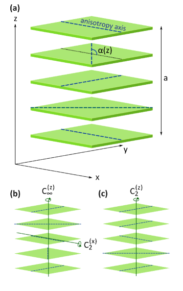
Figure 1: (a) A sketch of the multilayered structure composed of anisotropic layers rotated relative to each other. (b) Point symmetry axes in case of spiral symmetry. (c) Point symmetry axis for the arbitrary rotation of the layers $\alpha(z)$.

III Derivation of the effective material parameters: normal incidence scenario

In our theoretical analysis, we assume that the first anisotropic layer is located at $z=0$ possessing the permittivity tensor

$$\hat{\varepsilon}_{01}=\begin{pmatrix}\varepsilon_{1}&0&0\\ 0&\varepsilon_{2}&0\\ 0&0&\varepsilon_{3}\end{pmatrix}.$$ (6)

Other layers with identical properties are rotated by different angles $\alpha$ in $Oxy$ plane. Hence, the permittivity of the layer with the coordinate $z$ is given by

$$\begin{split}\hat{\varepsilon}(z)&=\hat{R}(\alpha)\hat{\varepsilon}_{01}\hat{R}^{-1}(\alpha)\\ =&\begin{pmatrix}\bar{\varepsilon}&0&0\\ 0&\bar{\varepsilon}&0\\ 0&0&\varepsilon_{3}\end{pmatrix}+\Delta\varepsilon\begin{pmatrix}-\cos(2\alpha)&-\sin(2\alpha)&0\\ -\sin(2\alpha)&\cos(2\alpha)&0\\ 0&0&0\end{pmatrix},\end{split}$$ (7)

where $\hat{R}$ matrix describes counterclockwise rotation with respect to $z$ axis

$$\hat{R}(\alpha)=\begin{pmatrix}\cos\alpha&-\sin\alpha&0\\ \sin\alpha&\cos\alpha&0\\ 0&0&1\end{pmatrix}\>,$$ (8)

$\bar{\varepsilon}=(\varepsilon_{1}+\varepsilon_{2})/2$ is the average permittivity, $\Delta\varepsilon=(\varepsilon_{2}-\varepsilon_{1})/2$ is the half-difference between the principal permittivity components and $b=2\pi/a$ is the reciprocal lattice period.

In the case of monochromatic fields and monochromatic external sources $\mathbf{j}$ Maxwell’s equations yield

$$\Delta\mathbf{E}-\nabla(\operatorname{div}\mathbf{E})+q^{2}\mathbf{D}=-\frac{4\pi\,i\,q}{c}\,\mathbf{j},$$ (9)

where $q=\omega/c$, $\omega$ is the frequency of the wave, $c$ is the speed of light and CGS system of units is employed.

Periodicity of the system allows to expand the electric field in the form

$$\mathbf{E}(\mathbf{r})=\sum_{n}\mathbf{E}_{n}\exp\left[i{\bf k}_{\bot}\cdot{\bf r}+i(k_{z}+nb)z\right],$$ (10)

where $\mathbf{E}_{n}$ are the Floquet harmonics of electric field, $\mathbf{k}$ is the wave vector with in-plane component $\mathbf{k}_{\bot}$ and the similar expansion is valid for the electric displacement $\mathbf{D}$.

Deriving the effective medium description, we focus on the behavior of the averaged fields represented by the zeroth order Floquet harmonic of the expansion Eq. (10). Assuming that the external current density $\mathbf{j}$ has only zeroth order Floquet harmonic $\mathbf{j}_{0}$, we aim to compute higher-order Floquet harmonics in terms of the averaged fields and recover the link between $\mathbf{D}_{0}$ and $\mathbf{E}_{0}$, which defines the effective material parameters of interest. In turn, the presence of external sources $\mathbf{j}$ allows to distinguish frequency and spatial dispersion as $\mathbf{k}$ and $\omega$ become independent.

To illustrate the above strategy, we consider first the scenario when the wave vector is orthogonal to the layers, $\mathbf{k}=(0,0,k_{z})^{\mathsf{T}}$, while electric field lies in the $Oxy$ plane: $\mathbf{E}=(E_{x},E_{y},0)^{\mathsf{T}}$. As the electric field is orthogonal to $\mathbf{k}$ and $\mathbf{k}+nb\,{\bf e}_{z}$, the problem simplifies, $\nabla\left(\mathop{\rm div}\nolimits{\mathbf{E}}\right)$ drops out from Eq. (9) and we immediately recover the connection between higher-order Floquet harmonics of electric field and displacement:

$$\mathbf{E}_{n}=\frac{q^{2}}{(k_{z}+nb)^{2}}\,\mathbf{D}_{n}\approx\frac{q^{2}}{n^{2}b^{2}}\left(1-\frac{2k_{z}}{nb}\right)\mathbf{D}_{n}+O(\xi^{4}),$$ (11)

where $\xi=q/b=a/\lambda$ is a small parameter and $n\neq 0$.

On the other hand, electric field and electric displacement at a given point are related to each other via the usual constitutive relation $\mathbf{D}(z)=\hat{\varepsilon}(z)\,\mathbf{E}(z)$. Expanding the permittivity in the Fourier series $\hat{\varepsilon}(z)=\sum\limits_{n}\hat{\varepsilon}_{n}\,e^{inbz}$ and using the Floquet expansion of the fields, Eq. (10), we recover

$$\mathbf{D}_{n}=\sum_{n^{\prime}}\hat{\varepsilon}_{n-n^{\prime}}\mathbf{E}_{n^{\prime}}=\hat{\varepsilon}_{n}\mathbf{E}_{0}+O(\xi^{2}).$$ (12)

Combining Eqs. (11) and (12), we deduce the averaged displacement in the form

$$\mathbf{D}_{0}=\sum_{n}\hat{\varepsilon}_{-n}\mathbf{E}_{n}=\hat{\varepsilon}_{0}\mathbf{E}_{0}+\sum_{n\neq 0}\hat{\varepsilon}_{-n}\mathbf{E}_{n}\approx$$

$$\approx\hat{\varepsilon}_{0}\mathbf{E}_{0}+\frac{q^{2}}{b^{2}}\sum_{n\neq 0}\frac{\hat{\varepsilon}_{-n}\hat{\varepsilon}_{n}}{n^{2}}\mathbf{E}_{0}-\frac{2k_{z}q^{2}}{b^{3}}\sum_{n\neq 0}\frac{\hat{\varepsilon}_{-n}\hat{\varepsilon}_{n}}{n^{3}}\mathbf{E}_{0}=$$

$$=\left[\hat{\varepsilon}_{0}+\frac{q^{2}}{b^{2}}{\sum_{n=1}^{\infty}\frac{\{\hat{\varepsilon}_{-n},\hat{\varepsilon}_{n}\}}{n^{2}}}\right]\mathbf{E}_{0}-\frac{2k_{z}q^{2}}{b^{3}}{\sum_{n=1}^{\infty}\frac{[\hat{\varepsilon}_{-n},\hat{\varepsilon}_{n}]}{n^{3}}}\mathbf{E}_{0},$$ (13)

where the terms proportional to $\xi^{4}$ or higher powers of small parameter $\xi$ are neglected.

Such connection between the averaged fields is a typical example of spatial dispersion, when the electric displacement depends not only on the field at the same point, but also on its spatial derivatives (see the term $\propto k_{z}$). However, the first derivative of $\mathbf{E}$ yields magnetic field $\mathbf{H}$ and therefore such corrections are equivalent to bianisotropy [16] with the material equations Eq. (1). The connection between the nonlocal permittivity tensor $\hat{\epsilon}(\omega,\mathbf{k})$ and local effective material parameters $\hat{\varepsilon}$ and $\hat{\kappa}$ reads [24]:

$$\hat{\epsilon}(\omega,\mathbf{k})=\left[\hat{\varepsilon}-\hat{\kappa}\hat{\kappa}^{\mathsf{T}}\right]+\frac{i}{q}\,\left[\hat{\kappa}\mathbf{k}^{\times}+\mathbf{k}^{\times}\hat{\kappa}^{\mathsf{T}}\right]\>,$$ (14)

where $\mathbf{k}_{il}=e_{ijl}\,k_{j}$ and $e_{ijl}$ is a fully antisymmetric tensor with $e_{123}=1$.

For the general structure of chirality tensor Eq. (5) and normal incidence geometry, spatial dispersion correction in Eq. (14) takes a simple form

$$\delta\hat{\epsilon}(\omega,\mathbf{k})=2i\kappa_{\text{eff}}k_{z}/q\,{\bf e}_{z}^{\times}\>,$$ (15)

where $\kappa_{\text{eff}}=(\kappa_{11}+\kappa_{22})/2$. To proceed further, we evaluate $\hat{\varepsilon}_{n}$ Fourier components with $n\not=0$ explicitly from Eq. (7):

$$\hat{\varepsilon}_{n}\equiv\frac{1}{a}\int_{0}^{a}\hat{\varepsilon}(z)e^{-inbz}dz=-\Delta\varepsilon\,\left(\sigma_{z}\,C_{n}+\sigma_{x}\,S_{n}\right)\>,$$ (16)

where we consider $xy$ subspace, $\sigma_{x}$ and $\sigma_{z}$ denote Pauli matrices and the dimensionless coefficients $C_{n}$ and $S_{n}$ are given by

$$C_{n}=\frac{1}{a}\,\int\limits_{0}^{a}\,e^{-inbz}\,\cos 2\alpha(z)\,dz\>,$$ (17)

$$S_{n}=\frac{1}{a}\,\int\limits_{0}^{a}\,e^{-inbz}\,\sin 2\alpha(z)\,dz$$ (18)

and depend on the specific way how the anisotropy axis is rotated from layer to layer.

Straightforward calculation and the comparison of Eqs. (13), (15) yield the general expression for effective chirality

$$\kappa_{\text{eff}}=-\frac{4\Delta\varepsilon^{2}\,q^{3}}{b^{3}}\,\sum\limits_{n=1}^{\infty}\,\frac{\operatorname{Im}\left(C_{n}\,S_{n}^{*}\right)}{n^{3}}\>,$$ (19)

while $xx$ and $yy$ components of effective permittivity read

$$\varepsilon_{\text{eff}}=\bar{\varepsilon}+\frac{2q^{2}\Delta\varepsilon^{2}}{b^{2}}\,\sum\limits_{n=1}^{\infty}\,\frac{|C_{n}|^{2}+|S_{n}|^{2}}{n^{2}}\>.$$ (20)

Equations (19),(20) define the effective material parameters of a multilayer for the arbitrary law of anisotropy axis rotation. Interestingly, the correction to the effective permittivity appears already in the second order in $\xi=q/b$, while chirality arises only in the third order vanishing in the subwavelength limit $\xi\ll 1$.

It is instructive to examine the case of spiral medium with a specific law of anisotropy axis rotation, Eq. (2). In this case, for $n\geq 1$ $C_{n}=1/2\,\delta_{n1}$ and $S_{n}=-i/2\,\delta_{n1}$ and thus

$$\varepsilon_{\text{eff}}=\bar{\varepsilon}+\Delta\varepsilon^{2}\frac{q^{2}}{b^{2}},$$ (21)

$$\kappa_{\text{eff}}=-\Delta\varepsilon^{2}\frac{q^{3}}{b^{3}}.$$ (22)

Note that the latter equations were obtained previously [19, 23] without using homogenization theory but examining the eigenmodes of a spiral medium instead (Supplementary Materials, Sec. I). Indeed, electromagnetic chirality is imprinted in the structure of the eigenmodes which have circular polarizations and different refractive indices

$$n_{\pm}=\sqrt{\varepsilon\mu}\pm\kappa,$$ (23)

which allows to probe chirality via eigenmode simulations.

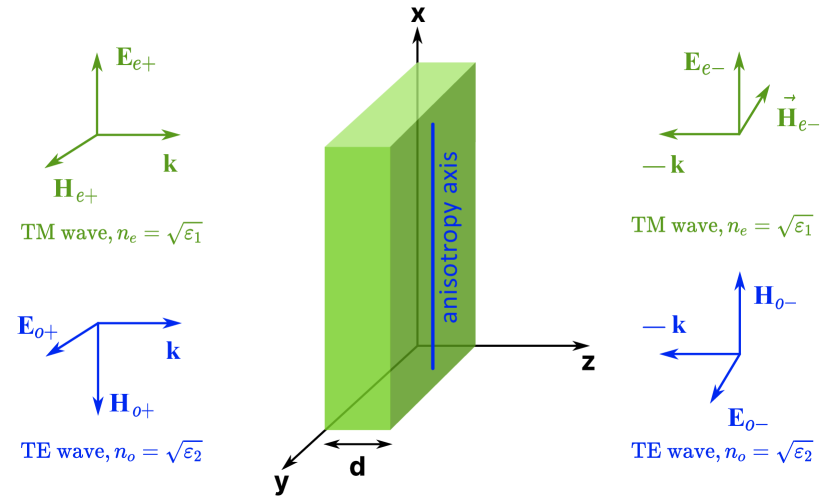
Figure 2: Reflection and transmission of waves in anisotropic dielectric slab and construction of the transfer matrix.

It should be stressed that the solution Eqs. (19), (20) presented here is more general and allows to compute chiral response in other physically relevant situations – for instance, when the unit cell of the lattice contains few anisotropic layers and the rotation of anisotropy axis from layer to layer is not continuous but rather stepwise (see Supplementary Materials, Sec. II).

IV Validation of the effective medium description

To test the validity of the effective medium description, we simulate multilayered metamaterial using rigorous transfer matrix method. We introduce the vector of the fields $\mathbf{v}=(E_{x},E_{y},H_{x},H_{y})^{\mathsf{T}}$ and define the transfer matrix as

$$\mathbf{v}(d)=\hat{M}(d)\,\mathbf{v}(0)\>.$$ (24)

Then, given the eigenmodes of anisotropic dielectric [Fig. 2], the tranfer matrix $\hat{M}(d)$ for the homogeneous slab with $x$-oriented anisotropy axis reads

$$\begin{pmatrix}\cos{(qn_{e}d)}&0&0&\frac{i}{n_{e}}\sin{(qn_{e}d)}\\ 0&\cos{(qn_{o}d)}&-\frac{i}{n_{0}}\sin{(qn_{o}d)}&0\\ 0&-in_{0}\sin{(qn_{o}d)}&\cos{(qn_{o}d)}&0\\ in_{e}\sin{(qn_{e}d)}&0&0&\cos{(qn_{e}d)}\end{pmatrix}.$$

If the layer is rotated, its transfer matrix is computed as

$$\hat{M}_{m}=\hat{T}(\alpha_{m})\hat{M}_{0}\hat{T}^{-1}(\alpha_{m}),$$

with

$$\hat{T}(\alpha)=\begin{pmatrix}R_{2}(\alpha)&0_{2}\\ 0_{2}&R_{2}(\alpha)\end{pmatrix}\>,$$

where $R_{2}(\alpha)$ is the $xy$ block of the rotation matrix Eq. (8) and $0_{2}$ is $2\times 2$ zero matrix. The transfer matrix for the lattice period is recovered by multiplying the matrices of all constituent layers

$$\hat{M}_{\text{period}}=\hat{M}_{N}\cdot\hat{M}_{N-1}\cdot...\cdot\hat{M}_{2}\cdot\hat{M}_{1}\cdot\hat{M}_{0}.$$ (25)

The eigenmodes of the periodic structure are found from the equation

$$\left[\hat{M}_{\text{period}}-e^{ik_{z}a}\right]\,\mathbf{v}(0)=0\>,$$ (26)

where the eigenvalues $k_{z}$ are related to the refractive indices of the eigenmodes, while the respective eigenvectors ${\bf v}$ define their polarization at the point $z=0$.

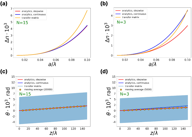
Figure 3: Probing the eigenmodes of a multilayered structure composed of anisotropic layers. (a,b) Refractive index difference for the two forward-propagating modes versus $a/\lambda$ ratio when the period consists of (a) $N=15$ and (b) $N=3$ layers, respectively. Orange, blue and red line depict the results of rigorous transfer matrix simulation and analytical calculation for the continuous and stepwise anisotropy axis rotation, respectively. (c,d) Polarization plane rotation for the linearly polarized wave propagating in the bulk metamaterial with $a/\lambda=0.01$. Light blue line depicts the results of transfer matrix simulation, orange dots correspond to the moving average over 200 and 500 layers, 10 dots are taken within each layer. Blue and red curves show the analytical results for the continuous and stepwise rotation of anisotropy axis. The permittivity of the layers is $\varepsilon_{1}=10$, $\varepsilon_{2}=7$. The overall number of periods is equal to 15000.

We solve Eq. (26) for experimentally relevant parameters [23] at normal incidence ($k_{z}=nq$). Assuming that the lattice period is formed by $N=15$ anisotropic layers with a uniform rotation of anistropy axis from layer to layer, in Fig. 3(a) we plot the difference of the refractive indices of the two forward-propagating eigenmodes which quantifies the effective chirality [see Eq. (23)]. As chirality is proportional to $(a/\lambda)^{3}$, $\Delta n$ is tiny in the deeply subwavelength region $\xi=a/\lambda\ll 1$. However, with the increase of $\xi$ up to 0.06, $\Delta n$ grows rapidly. At this point, the developed perturbation theory is no longer valid, and the discrepancy between the effective medium model and transfer matrix method mounts. At the same time, the assumption about the continuous rotation of anisotropy axis remains good approximation for $N=15$ layers in the period.

A qualitatively similar behavior of $\Delta n$ is observed, when the period of the lattice includes just $N=3$ layers [Fig.  3(b)]. In this case, however, one has to take into account that the rotation of anisotropy axis from layer to layer is not continuous, but rather stepwise, as further analyzed in the Supplementary Materials, Sec. II.

Another aspect of chirality is the rotation of polarization plane of the linearly polarized wave propagating in the chiral medium. Decomposing the wave into two circularly polarized modes and taking into account the difference of the refractive indices, Eq. (23), we recover the rotation $\theta=-q\kappa_{\text{eff}}\,z$. The results for $N=15$ and $N=3$ layers in the period for the fixed ratio $a/\lambda=0.01$ are presented in Fig. 3(c,d). We compare these results with the transfer matrix calculation. In the latter case, however, polarization varies strongly within the layer, being elliptical in the general case. We compute the angle of rotation at each point as

$$\theta=\frac{1}{2}\arctan{\left(\frac{2E_{tx}E_{ty}\cos(\Delta\phi)}{E_{tx}^{2}-E_{ty}^{2}}\right)},$$

where $E_{tx}$ and $E_{ty}$ are the amplitudes of light transmitted through each layer and $\Delta\phi$ is the phase difference between those components. These results are depicted by the thin blue line in Fig. 3(c,d) creating a uniform shading due to the rapid oscillations of polarization within the metamaterial period. Next we average the rotation angle taking a sliding averaging window. The obtained averaged results are in full agreement with the analytical theory demonstrating the rotation of polarization plane linearly growing with distance indicating the onset of effective chirality.

V Maximization of effective chirality

To illustrate the power of the obtained general solution for chirality $\kappa_{\text{eff}}$, we explore the following problem. Assume that the multilayered structure is composed of very thin layers with the given principal components of permittivity tensor $\varepsilon_{1}$, $\varepsilon_{2}$, and the period $a$ of the lattice is fixed. In this setting, emergent chirality depends on the orientation of the layers described by the periodic function $\alpha(z)$. Below, we aim to find the arrangement of the layers maximizing chiral response $\kappa_{\text{eff}}$.

To do so, we compare Eqs. (13) and (15) and present chirality in the form

$$\kappa_{\text{eff}}\,\mathbf{e}_{z}^{\times}=i\frac{q^{3}}{b^{3}}\sum_{n\not=0}\frac{1}{n^{3}}\hat{\varepsilon}_{-n}\hat{\varepsilon}_{n}\>.$$ (27)

For our analysis, it is convenient to transform Eq. (27) replacing the summation of the Fourier harmonics by the integration in the real space. Assuming that arbitrary periodic function $f(z)$ is presented in the form

$$f(z)=\sum_{n=-\infty}^{\infty}f_{n}e^{inbz}$$

we introduce the operator $\mathcal{J}$ acting in the Fourier space as

$$(\mathcal{J}f)_{n}=\begin{cases}\frac{1}{ibn}f_{n},&n\neq 0\\ 0,&n=0.\end{cases}$$ (28)

Essentially, this substracts the average from the function $f(z)$, integrates it over the interval $[0,z]$ and substracts the average from the resulting function. Accordingly, in the real space the operator $\mathcal{J}$ acts as

$$\mathcal{J}f(z)=\int\limits_{0}^{a}\,K_{1}\left(\frac{z-z^{\prime}}{a}\right)\,f(z^{\prime})\,dz^{\prime}\>,$$ (29)

$$K_{1}(\xi)=\frac{1}{2}\,\text{sign}\left(\xi\right)-\xi\>.$$ (30)

Having Eq. (29), it is straightforward to compute the repeated action of the operator $\mathcal{J}$. For instance,

$$\mathcal{J}^{3}f(z)=a^{2}\,\int\limits_{0}^{a}\,K_{3}\left(\frac{z-z^{\prime}}{a}\right)\,f(z^{\prime})\,dz^{\prime}\>,$$ (31)

$$K_{3}(\xi)=-\frac{1}{12}\,\xi\left(1-3|\xi|+2\xi^{2}\right)\>.$$ (32)

Yet another ingredient needed for our calculation are the definitions of the scalar product and norm

$$\langle f,g\rangle =\int_{0}^{a}f^{*}(z)g(z)dz=a\sum_{n=-\infty}^{\infty}f_{n}^{*}g_{n},$$ (33)

$$\|f\|^{2} =\langle f,f\rangle=a\sum_{n=-\infty}^{\infty}|f_{n}|^{2}\>.$$ (34)

As the permittivity tensor of the layers is real, $\hat{\varepsilon}_{-n}=\hat{\varepsilon}_{n}^{*}$ and therefore

$$\kappa_{\text{eff}}\,\mathbf{e}_{z}^{\times}=q^{3}\,\sum_{n\not=0}\hat{\varepsilon}_{n}^{*}\,\frac{\hat{\varepsilon}_{n}}{(ibn)^{3}}=q^{3}\,\sum_{n\not=0}\hat{\varepsilon}_{n}^{*}\,\left(\mathcal{J}^{3}\hat{\varepsilon}\right)_{n}$$

$$=\frac{q^{3}}{a}\int\limits_{0}^{a}\hat{\varepsilon}(z)\,\left[\mathcal{J}^{3}\hat{\varepsilon}(z)\right]\,dz$$

$$=q^{3}\,a\int\limits_{0}^{a}\int\limits_{0}^{a}\,\hat{\varepsilon}(z)\,K_{3}\left(\frac{z-z^{\prime}}{a}\right)\,\hat{\varepsilon}(z^{\prime})\,dz^{\prime}dz$$

$$=\frac{q^{3}\,a}{2}\int\limits_{0}^{a}\int\limits_{0}^{a}\,K_{3}\left(\frac{z-z^{\prime}}{a}\right)\,\left[\hat{\varepsilon}(z),\hat{\varepsilon}(z^{\prime})\right]\,dz^{\prime}dz\>.$$ (35)

Straightforward calculation of the commutator using Eq. (7) yields

$$[\hat{\varepsilon}(z),\hat{\varepsilon}(z^{\prime})]=2\Delta\varepsilon^{2}\operatorname{Im}\left(e^{2i\alpha(z)}\,e^{-2i\alpha(z^{\prime})}\right)\mathbf{e}_{z}^{\times}$$ (36)

giving an explicit formula for chirality

$$\kappa_{\text{eff}}=q^{3}a\Delta\varepsilon^{2}\,\operatorname{Im}\int\limits_{0}^{a}\int\limits_{0}^{a}\,K_{3}\left(\frac{z-z^{\prime}}{a}\right)\,e^{2i\alpha(z)}\,e^{-2i\alpha(z^{\prime})}\,dzdz^{\prime}$$

$$=\frac{q^{3}}{a}\Delta\varepsilon^{2}\,\operatorname{Im}\left<\psi,\mathcal{J}^{3}\psi\right>\>,$$ (37)

where $\psi(z)=\exp(-2i\alpha(z))$ is an auxiliary scalar function. The latter expression can be readily estimated as follows:

$$|\operatorname{Im}\langle\psi,\mathcal{J}^{3}\psi\rangle| =a\left|\operatorname{Im}\sum_{n\neq 0}\frac{\psi^{*}_{n}\psi_{n}}{-ib^{3}n^{3}}\right|$$

$$\leq\frac{a}{b^{3}}\sum_{n\neq 0}\left|\frac{1}{n^{3}}\right|\psi^{*}_{n}\psi_{n}\leq\frac{a}{b^{3}}\sum_{n}\psi^{*}_{n}\psi_{n}$$

$$=\frac{1}{b^{3}}\|\psi\|^{2}=\frac{a}{b^{3}}$$

Hence, an upper bound for chirality $\kappa_{\text{eff}}$ reads:

$$|\kappa_{\text{eff}}|\leq\frac{q^{3}}{b^{3}}\Delta\varepsilon^{2}\>.$$ (38)

This value is achieved for $\psi=e^{-ibz}$. Thus, we conclude that the arrangement of the layers maximizing chiral response is the continuous rotation of anisotropy axis, i.e. spiral symmetry.

To illustrate that, we chose a specific set of $\alpha(z)$ functions, parameterized by $\gamma$ as follows:

$$\alpha_{\gamma}(z)=\pi\left[\frac{z}{a}+\gamma\frac{z}{a}\left(1-\frac{z}{a}\right)\right]$$ (39)

In Fig. 4 we plot the dependence of effective chirality $\kappa_{\text{eff}}$ on $\gamma$. We chose a range $[-1,1]$ for $\gamma$, so that the rotation angle $\alpha(z)$ changes monotonously with $z$. As anticipated from our general analysis, chiral response reaches its maximum exactly for $\gamma=0$.

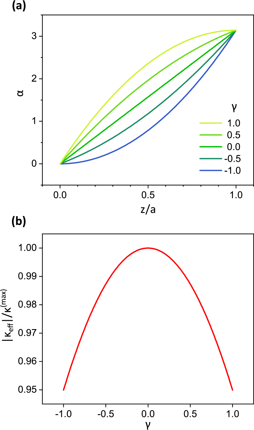
Figure 4: Illustration of effective chirality maximization. (a) Various laws of anisotropy axis rotation $\alpha(z)$ distinguished by the $\gamma$ parameter. (b) Relative effective chirality as a function of $\gamma$. Chirality reaches its maximum for the uniform rotation of anisotropy axis, i.e. in case of spiral symmetry.

VI Reconstruction of the full chirality tensor

In this section, we generalize our treatment and examine an arbitrary direction of $\mathbf{k}$ vector. In experimental situation, this corresponds to the oblique incidence scenario. For simplicity, we assume that the anisotropy axis rotates continuously according to Eq. (2), so that the effective chirality tensor has the diagonal structure, Eq. (4). While $\kappa_{11}$ component is calculated above, $\kappa_{33}$ term is only manifested at oblique incidence.

As we consider an unbounded medium with spiral symmetry, without loss of generality we can rotate the coordinate system and assume that the wave vector is $\mathbf{k}=(k_{x},0,k_{z})^{\mathsf{T}}$, while all components of electric field are nonzero $\mathbf{E}=(E_{x},E_{y},E_{z})^{\mathsf{T}}$. In such setting, the wave equation Eq. (9) results in the system:

$$-(k_{z}+nb)^{2}E_{nx}+k_{x}(k_{z}+nb)E_{nz}+q^{2}D_{nx}=0,$$ (40)

$$k_{x}(k_{z}+nb)E_{nx}-k_{x}^{2}E_{nz}+q^{2}D_{nz}=0,$$ (41)

$$-(k_{z}+nb)^{2}E_{ny}-k_{x}^{2}E_{ny}+q^{2}D_{ny}=0.$$ (42)

Equations (40) and (41) can be combined to yield

$$k_{x}D_{nx}+(k_{z}+nb)D_{nz}=0.$$ (43)

In turn, the material equation for the Floquet harmonics of electric field reads

$$\mathbf{D}_{n}=\sum_{m}\hat{\varepsilon}_{n-m}\mathbf{E}_{m},$$ (44)

or, alternatively, introducing the inverse permittivity $\hat{\zeta}$,

$$\mathbf{E}_{n}=\sum_{m}\hat{\zeta}_{n-m}\mathbf{D}_{m}.$$ (45)

Next we employ the perturbation theory with the small parameter $\xi=a/\lambda$ presenting the Floquet harmonics with $n\not=0$ as a series

$$\begin{cases}E_{ni}=E_{ni}^{(0)}+\xi E_{ni}^{(1)}+\xi^{2}E_{ni}^{(2)}+...\\ D_{ni}=D_{ni}^{(0)}+\xi D_{ni}^{(1)}+\xi^{2}D_{ni}^{(2)}+...\end{cases}$$ (46)

where index $i=x,y,z$ labels the Cartesian component.

Performing the calculations similarly to the normal incidence case (see details in Supplementary Materials, Section III), we recover the effective material parameters:

$$\hat{\varepsilon}_{\text{eff}}=\begin{pmatrix}\bar{\varepsilon}+\frac{\Delta\varepsilon^{2}}{2b^{2}}\left(2q^{2}-\frac{k_{x}^{2}}{\varepsilon_{3}}\right)&0&0\\ 0&\bar{\varepsilon}+\frac{\Delta\varepsilon^{2}}{2b^{2}}\left(2q^{2}-\frac{k_{x}^{2}}{\varepsilon_{3}}\right)&0\\ 0&0&\varepsilon_{3}\end{pmatrix},$$

$$\hat{\kappa}_{\text{eff}}=-\frac{q}{2}\frac{\Delta\varepsilon^{2}}{b^{3}}\left(2q^{2}-\frac{k_{x}^{2}}{\varepsilon_{3}}\right)\begin{pmatrix}1&0&0\\ 0&1&0\\ 0&0&-1\end{pmatrix}.$$ (47)

Interestingly, effective permittivity tensor $\hat{\varepsilon}_{\text{eff}}$ acquires second-order spatial dispersion correction, while effective chirality is cubic in $\xi$ and also contains spatial dispersion contribution. Equation (47) suggests that $\kappa_{33}$ component is nonzero and has different sign compared to $\kappa_{11}$.

To validate such behavior of effective chiral response, we analyze both refractive indices and polarizations of the modes supported by the structure at oblique incidence.

First, we fix the frequency $q=\omega/c$ and calculate the isofrequency contour in the $Oxz$ plane. To isolate the effects due to chirality and spatial dispersion, we subtract from the propagation constant $k_{z}$ its dominant part $k_{z}^{\text{(u)}}$ – a value obtained for a uniaxial non-chiral crystal with

$$\hat{\varepsilon}^{\text{(u)}}=\text{diag}\left(\bar{\varepsilon},\bar{\varepsilon},\varepsilon_{3}\right),\quad\hat{\kappa}^{\text{(u)}}=\hat{0}\>.$$ (48)

Figure 5(a) shows the corrections to the propagation constants of two forward-propagating ($k_{z}>0$) modes at different incidence angles quantified by the $k_{x}$. We observe that the effective medium model correctly reproduces $k_{z}$ values at all incidence angles.

To support our effective medium model further, we calculate the polarizations of the same modes quantifying them by the Stokes parameters defined as

$$S_{0} =|E_{0x^{\prime}}|^{2}+|E_{0y^{\prime}}|^{2},$$ (49)

$$S_{1} =|E_{0x^{\prime}}|^{2}-|E_{0y^{\prime}}|^{2},$$ (50)

$$S_{2} =2\operatorname{Re}\left(E_{0x^{\prime}}E_{0y^{\prime}}^{*}\right),$$ (51)

$$S_{3} =-2\operatorname{Im}\left(E_{0x^{\prime}}E_{0y^{\prime}}^{*}\right).$$ (52)

Here, $\mathbf{E}_{0}$ denotes the averaged field calculated as

$$\mathbf{E}_{0}=\frac{1}{a}\int_{0}^{a}\mathbf{E}(z)e^{-ik_{z}z}dz,$$

and $k_{z}$ is recovered from the eigenmode calculation, Eq.(26). The Stokes parameters are evaluated in the plane $Ox^{\prime}y^{\prime}$ spanned by $\operatorname{Re}\mathbf{E}_{0}$ and $\operatorname{Im}\mathbf{E}_{0}$ vectors; $Ox^{\prime}$ corresponds to the projection of $Ox$ axis onto the polarization plane, while $Oy^{\prime}$ axis satisfies the conditions

$$[\mathbf{e}_{x^{\prime}}\times\mathbf{e}_{y^{\prime}}]\cdot\mathbf{e}_{z}>0,\quad\mathbf{e}_{x^{\prime}}\cdot\mathbf{e}_{y^{\prime}}=0.$$

This choice of the coordinate system ensures that $S_{2}=0$.

In our calculation, we choose $\varepsilon_{3}=\bar{\varepsilon}$ in order to mitigate the effect of optical anisotropy in the limit $\xi\to 0$ and isolate the influence of $\kappa_{33}$ chirality component. We perform the effective medium calculation for various $k_{x}$ and for the set of chirality tensors with different values of $\kappa_{33}$ component: $\kappa_{33}=-s\,\kappa_{11}$ comparing the results for a mode with a larger $k_{z}$ in Fig. 5(b,c). Comparing the analytical results with the transfer matrix calculation, we recover that the best approximation corresponds to $s=1$, meaning that $\kappa_{33}=-\kappa_{11}$ in agreement with the theoretical prediction.

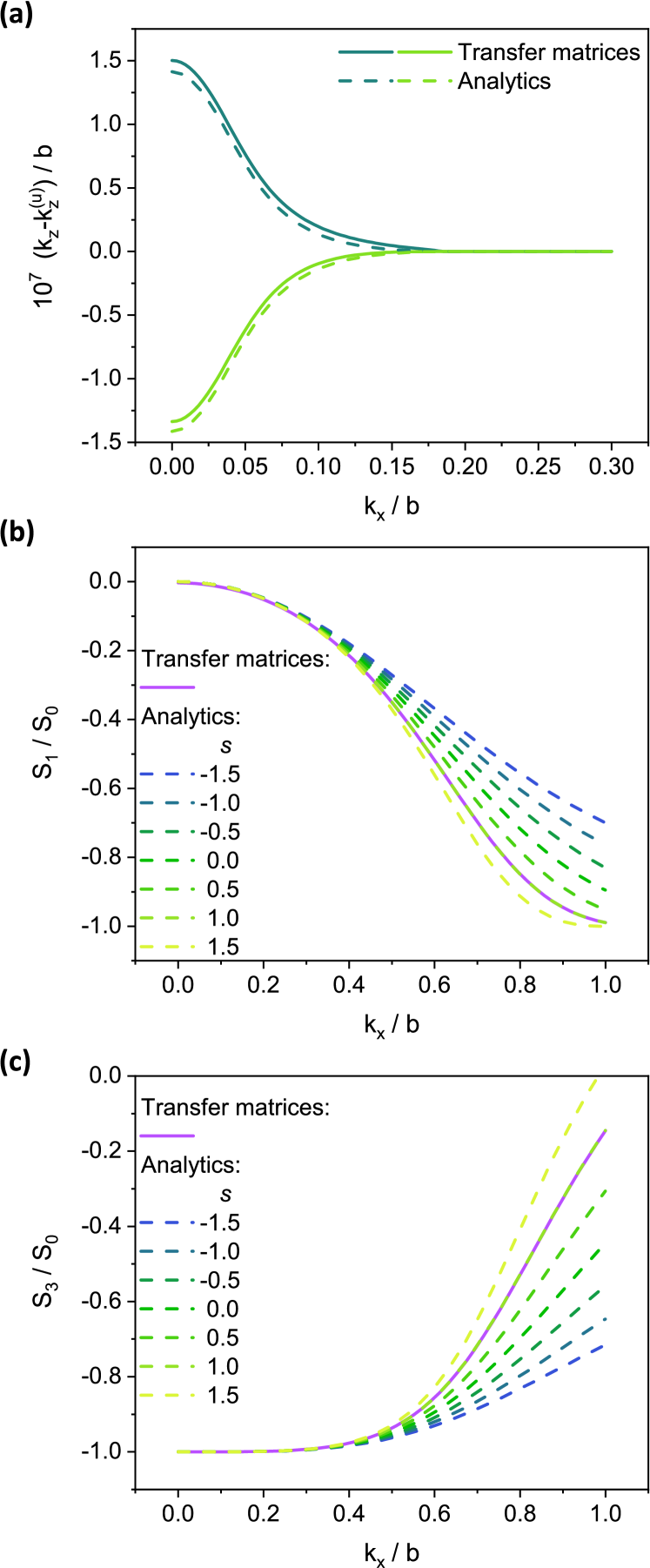
Figure 5: Validation of effective medium description at oblique incidence. (a) Isofrequency contour in $Oxz$ plane with $k_{z}^{(u)}$ for a uniaxial crystal subtracted. $a/\lambda=0.01$ is fixed, the permittivity values for a single layer are $\varepsilon_{1}=10.0$, $\varepsilon_{2}=7.0$, $\varepsilon_{3}=8.5$. (b, c) Stokes parameters for a single eigenmode with the larger $k_{z}$, calculated by the transfer matrix method, superposed with analytical results corresponding to different values of $\kappa_{33}$. $a/\lambda=0.06$, layer permittivities are the same as above.

VII Discussion and conclusions

In summary, we have derived a complete effective medium description of the multilayered structure composed of anisotropic layers rotated relative to each other. Our description captures the metamaterial regime when the lattice period is much smaller than the wavelength. In such case, electromagnetic chirality is proportional to $\left(a/\lambda\right)^{3}$ and features spatial dispersion contribution at oblique incidence.

As we proved, continuous rotation of anisotropy axis from layer to layer maximizes the effective chirality compared to any other configuration with the same lattice period $a$ and permittivities of the individual layers $\varepsilon_{1}$ and $\varepsilon_{2}$.

While our analysis provides insights into the emergence of effective chirality in a stack of anisotropic layers, we believe that our methodology is more general and enables understanding of other layered geometries featuring more exotic responses. It could also pave a way to the reverse engineering of metamaterial structures with the prescribed effective properties.

References

- Veselago [1968] V. G. Veselago, The electrodynamics of substances with simultaneously negative values of and , Soviet Physics Uspekhi 10, 509 (1968).
- Eleftheriades and Balmain [2005] G. V. Eleftheriades and K. G. Balmain, Negative-Refraction Metamaterials: Fundamental Principles and Applications (John Wiley & Sons, New Jersey, 2005).
- Marques et al. [2008] R. Marques, F. Martin, and M. Sorolla, Metamaterials with negative parameters (John Wiley & Sons, New Jersey, 2008).
- Belotelov et al. [2007] V. I. Belotelov, L. L. Doskolovich, and A. K. Zvezdin, Extraordinary Magneto-Optical Effects and Transmission through Metal-Dielectric Plasmonic Systems, Physical Review Letters 98, 077401 (2007).
- Asadchy et al. [2018] V. S. Asadchy, A. Díaz-Rubio, and S. A. Tretyakov, Bianisotropic metasurfaces: physics and applications, Nanophotonics 7, 1069 (2018).
- Belov et al. [2003] P. A. Belov, R. Marqués, S. I. Maslovski, I. S. Nefedov, M. Silveirinha, C. R. Simovski, and S. A. Tretyakov, Strong spatial dispersion in wire media in the very large wavelength limit, Physical Review B 67, 113103 (2003).
- Orlov et al. [2011] A. A. Orlov, P. M. Voroshilov, P. A. Belov, and Y. S. Kivshar, Engineered optical nonlocality in nanostructured metamaterials, Physical Review B 84, 045424 (2011).
- Shaposhnikov et al. [2023] L. Shaposhnikov, M. Mazanov, D. A. Bobylev, F. Wilczek, and M. A. Gorlach, Emergent axion response in multilayered metamaterials, Physical Review B 108, 115101 (2023).
- Safaei Jazi et al. [2024] S. Safaei Jazi, I. Faniayeu, R. Cichelero, D. C. Tzarouchis, M. M. Asgari, A. Dmitriev, S. Fan, and V. Asadchy, Optical Tellegen metamaterial with spontaneous magnetization, Nature Communications 15, 1293 (2024).
- Semnani et al. [2020] B. Semnani, J. Flannery, R. Al Maruf, and M. Bajcsy, Spin-preserving chiral photonic crystal mirror, Light: Science & Applications 9, 23 (2020).
- Voronin et al. [2022] K. Voronin, A. S. Taradin, M. V. Gorkunov, and D. G. Baranov, Single-Handedness Chiral Optical Cavities, ACS Photonics 9, 2652 (2022).
- Baranov et al. [2023] D. G. Baranov, C. Schäfer, and M. V. Gorkunov, Toward Molecular Chiral Polaritons, ACS Photonics 10, 2440 (2023).
- Tang and Cohen [2010] Y. Tang and A. E. Cohen, Optical Chirality and Its Interaction with Matter, Physical Review Letters 104, 163901 (2010).
- Fernandez-Corbaton et al. [2016] I. Fernandez-Corbaton, M. Fruhnert, and C. Rockstuhl, Objects of Maximum Electromagnetic Chirality, Physical Review X 6, 031013 (2016).
- Chen et al. [2024] W. Chen, Z. Wang, M. V. Gorkunov, J. Qin, R. Wang, C. Wang, D. Wu, J. Chu, X. Wang, Y. Kivshar, and Y. Chen, Uncovering Maximum Chirality in Resonant Nanostructures, Nano Letters 24, 9643 (2024).
- Serdyukov et al. [2001] A. Serdyukov, I. Semchenko, S. Tretyakov, and A. Sihvola, Electromagnetics of Bi-anisotropic Materials: Theory and Applications (Gordon and Breach Science Publishers, Amsterdam, 2001).
- Yin et al. [2013] X. Yin, M. Schäferling, B. Metzger, and H. Giessen, Interpreting Chiral Nanophotonic Spectra: The Plasmonic Born–Kuhn Model, Nano Letters 13, 6238 (2013).
- Barron [2004] L. Barron, Molecular Light Scattering and Optical Activity, 2nd ed. (Cambridge University Press, Cambridge, UK, 2004).
- Vetrov et al. [2020] S. Y. Vetrov, I. V. Timofeev, and V. F. Shabanov, Localized modes in chiral photonic structures, Physics-Uspekhi 63, 33 (2020).
- Rebholz et al. [2024] L. Rebholz, M. Krstić, B. Zerulla, M. Pawlak, W. Lewandowski, I. Fernandez-Corbaton, and C. Rockstuhl, Separating the Material and Geometry Contribution to the Circular Dichroism of Chiral Objects Made from Chiral Media, ACS Photonics 11, 1771 (2024).
- de Gennes and Prost [1993] P. G. de Gennes and J. Prost, The Physics of Liquid Crystals (Clarendon Press, Oxford, England, UK, 1993).
- Khoo [2022] I.-C. Khoo, Liquid Crystals, 3rd Edition (Wiley, Hoboken, NJ, USA, 2022).
- Voronin et al. [2024] K. V. Voronin, A. N. Toksumakov, G. A. Ermolaev, A. S. Slavich, M. K. Tatmyshevskiy, S. M. Novikov, A. A. Vyshnevyy, A. V. Arsenin, K. S. Novoselov, D. A. Ghazaryan, et al., Chiral Photonic Super-Crystals Based on Helical van der Waals Homostructures, Laser & Photonics Reviews 18, 2301113 (2024).
- Silveirinha [2007] M. G. Silveirinha, Metamaterial homogenization approach with application to the characterization of microstructured composites with negative parameters, Physical Review B 75, 115104 (2007).
- Gorlach and Lapine [2020] M. A. Gorlach and M. Lapine, Boundary conditions for the effective-medium description of subwavelength multilayered structures, Physical Review B 101, 075127 (2020).