Optimizing DNN Inference on Multi-Accelerator SoCs at Training-time

Abstract

The demand for executing Deep Neural Networks (DNNs) with low latency and minimal power consumption at the edge has led to the development of advanced heterogeneous Systems-on-Chips (SoCs) that incorporate multiple specialized computing units (CUs), such as accelerators. Offloading DNN computations to a specific CU from the available set often exposes accuracy vs efficiency trade-offs, due to differences in their supported operations (e.g., standard vs. depthwise convolution) or data representations (e.g., more/less aggressively quantized). A challenging yet unresolved issue is how to map a DNN onto these multi-CU systems to maximally exploit the parallelization possibilities while taking accuracy into account. To address this problem, we present ODiMO, a hardware-aware tool that efficiently explores fine-grain mapping of DNNs among various on-chip CUs, during the training phase. ODiMO strategically splits individual layers of the neural network and executes them in parallel on the multiple available CUs, aiming to balance the total inference energy consumption or latency with the resulting accuracy, impacted by the unique features of the different hardware units. We test our approach on CIFAR-10, CIFAR-100, and ImageNet, targeting two open-source heterogeneous SoCs, i.e., DIANA and Darkside. We obtain a rich collection of Pareto-optimal networks in the accuracy vs. energy or latency space. We show that ODiMO reduces the latency of a DNN executed on the Darkside SoC by up to $8\times$ at iso-accuracy, compared to manual heuristic mappings. When targeting energy, on the same SoC, ODiMO produced up to $50.8\times$ more efficient mappings, with minimal accuracy drop ($<0.3\%$).

I Introduction

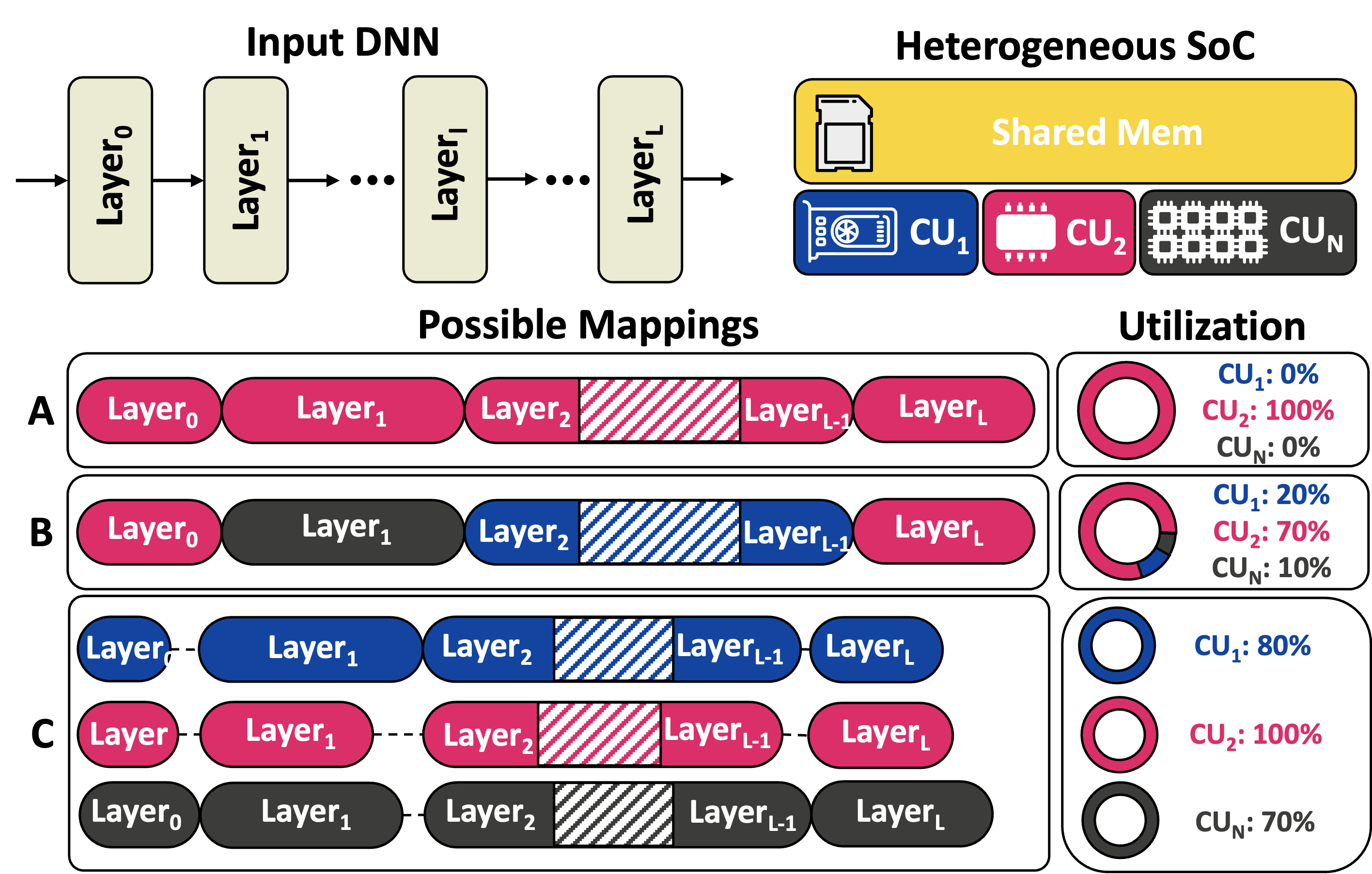
Figure 1: Different possible execution strategies of a DNN on a Heterogeneous SoC with shared memory. Strategy A offloads the DNN computation to a single CU. Strategy B uses a layer-wise scheme where each layer can be computed by one of the available CU. Strategy C is the intra-layer mapping scheme enabled by ODiMO, where the computation of each layer can be split among the different CUs.

Deploying DNNs for inference at the edge offers well-known advantages in terms of latency, predictability, energy consumption, and data privacy [1, 2]. However, the execution of computationally intensive DNNs on edge devices, which operate under stringent energy and memory constraints, poses a significant challenge. Current research addresses this problem in multiple, complementary ways. On the software side, various optimization techniques are employed to enhance the efficiency and accuracy of DNN models. These include Neural Architecture Search (NAS), which automates the design of DNN architectures under specified resource limits, pruning, which reduces the model size by removing redundant parameters, and quantization, which decreases the precision of the model weights and activations to lower computational demands and memory usage [2, 3, 4]. On the hardware side, efficiency is mostly improved through specialization. This involves the design and integration of heterogeneous Systems-on-Chip (SoCs) that incorporate domain-specific Computing Units (CUs) dedicated to DNN processing. These specialized hardware accelerators are tailored to handle specific computational patterns of DNN workloads, thereby significantly enhancing performance and/or energy efficiency [5, 6, 7, 8, 9], while sacrificing generality. In this work, we concentrate on heterogeneous SoCs architectures that present multiple CUs, communicating with each other through a shared on-chip memory (depicted in yellow in Fig. 1). Nonetheless, this work could be easily extended to any SoC with private CUs’ memories by taking into account the cost of broadcasting load and store operations among them.

Optimizing a DNN model for execution on these multi-CU systems remains a significant challenge. Traditionally, entire networks are executed on a single CU, as depicted Fig. 1 (Mapping A). More recent research has explored multi-CU inference [10, 11, 12, 6, 13, 14] with layer-wise partitioning (as in Mapping B). However, layer-wise partitioning leads to suboptimal hardware utilization, since for a standard sequential DNN, only one CU is active at any time. The possibility of partitioning at a finer grain, with each layer partitioned among multiple CUs (as in Mapping C of Fig. 1) is studied almost exclusively for the case of homogeneous CUs (e.g., multiple GPUs/TPUs) [15, 16], and still under-explored for systems with heterogeneous accelerators. Moreover, these studies generally assume that all CUs can execute all layers of a DNN, and deliver equally accurate results. However, this assumption does not hold in many real-world cases [8, 7, 9]. A notable counter-example are SoCs that incorporate both Digital and Analog In-Memory Computing (AIMC) CUs [7, 8]. AIMC can be faster and more energy-efficient, but produces approximated results due to the use of extreme quantization bit-width for weights, such as binary or ternary levels. In contrast, digital CUs, while slower and more energy-hungry, handle data with higher numerical precision and thus deliver more accurate results. Other SoCs [9] are equipped with CUs that can only execute specific DNN layers, such as depthwise convolutions. Using these CUs implies constraining the DNN to certain architectural patterns, which again can affect the accuracy (usually in exchange for improved efficiency).

In this work, which extends [17], we present One-shot Differentiable Mapping Optimizer (ODiMO) a novel approach to optimize and map DNN execution onto heterogeneous systems. In ODiMO, the mapping problem is framed as a training-time optimization where both functional (i.e., task performance) and non-functional (i.e., energy efficiency or latency) properties of each CU are taken into account, thus enabling the discovery of accurate yet efficient mappings. The main technical novelties of this work are detailed below:

• Our method operates at fine grain, using a gradient-based search technique at training time, to divide each DNN layer into sub-layers, which are then executed in parallel by various CUs, as depicted in Mapping C of Fig. 1. By considering potential accuracy losses due to quantization or layer type selection (e.g., normal convolution vs depthwise convolution), our approach aims to balance the tradeoff between accuracy and energy consumption or latency through the use of analytical and differentiable hardware-aware cost models.

• We evaluate the proposed approach on three well-known edge-relevant benchmarks from computer vision, namely CIFAR-10, CIFAR-100, and ImageNet. On these three datasets, we use ODiMO to explore mappings for two state-of-the-art open-source heterogeneous SoC designs, i.e., DIANA [8] and Darkside [9].

• Thanks to our fine-grain mapping discovery procedure we obtain novel solutions that outperform manual heuristic mappings. In particular, ODiMO improves latency by up to $4.9\times$/$8\times$ on DIANA and Darkside respectively, with an accuracy drop $<2\%$/no-accuracy drop compared to manual heuristic mappings. Similarly, ODiMO improves DIANA’s/Darkside’s energy efficiency, by up to $1.41\times$/$50.8\times$ with an accuracy drop $<0.5\%$.

Our code is open-sourced at: https://github.com/eml-eda/odimo-journal. The rest of the paper is structured as follows. Sec. II summarizes the required background concepts, while Sec. III covers the most relevant works related to our research. Sec. IV discusses the proposed methodology, which is experimentally validated in Sec. V. Finally, Sec. VI concludes the manuscript.

II Background

II-A Specialized hardware for edge DNN inference

In recent years, specialized architectures for DNN processing at the edge have proliferated, with numerous designs emerging from both industry and academia [18]. Many modern SoCs feature multiple specialized CUs capable of executing DNN layers with varying trade-offs in terms of latency, throughput, energy consumption, and accuracy. For instance, the Jetson AGX Xavier series from NVIDIA is a commercial device including an 8-core ARM CPU, an NVIDIA Volta GPU with 512 CUDA cores, and two NVIDIA Deep Learning Accelerators (NVDLAs). Users can distribute the workload between the GPU, which is faster but more energy-intensive, and the NVDLAs, which are slightly slower but more efficient [6]. Another commercial alternative is represented by the GAP9  SoC which includes a cluster of 8 general purpose cores based on the RISC-V ISA along with the Neural Engine 16 [19], a custom accelerator tailored to execute specific convolutional kernels with varying integer precision from 2 to 8 bits.

A similar architecture is used by Darkside [9], an academic and open-source design. Darkside includes an 8-core cluster of general-purpose RISC-V processors supporting integer arithmetic along with a custom CU, the Depthwise Convolution Engine (DWE). The DWE accelerates depthwise convolutions, an operation notoriously characterized by low arithmetic intensity and thus poor performance on general-purpose cores. The cluster and the DWE share an L1 memory composed of 32 4-kB SRAM banks capable of serving up to 32 requests in parallel. The memory hierarchy is completed by 256 kB of L2 accessed through a dedicated Direct Memory Access (DMA) co-processor. Moreover, Darkside also includes a 16-bit floating-point Tensor Product Engine (TPE) originally proposed to enable on-device learning.

Another emerging paradigm towards heterogeneity is represented by SoCs including CUs based on Near-Memory Computing (NMC) and Analog In-Memory Computing (AIMC). In the architecture presented in [7], a control CPU assigns the workload to either a 590k-cell AIMC CU, optimized for 1-bit multiply-and-accumulate (MAC) operations, or a digital NMC CU, which supports variable precision from 1 to 8 bits. Choosing between these two CUs involves a trade-off, as the NMC offers potentially higher accuracy at the cost of increased latency and energy consumption. Similarly, the DIANA architecture described in [8] incorporates a single-core RISC-V CPU as control processor, and two distinct DNN-specific CUs. One is a 16$\times$16 grid of digital processing elements that perform MACs at 8-bit precision and include a 64 kB weight memory, while the other is a 500k-cell AIMC CU with ternary weights. Both CUs share a dedicated 256 kB L1 memory, accessed via DMA.

In this work, we consider DIANA and Darkside as target HW platforms as two representatives of the heterogeneous edge SoCs landscape, different from each other. In particular, DIANA includes two CUs supporting different quantization precision, whereas Darkside includes a unit supporting only a specific layer type (the DWE). Nonetheless, all techniques discussed in this paper are sufficiently general to be applicable to other platforms too.

II-B Training-time Optimization of DNNs

Over the years, coupled with the introduction of new specialized SoCs, many DNN optimization strategies have been developed to build lightweight networks appropriate to be deployed on edge devices. Initially, the design of architectures encompassed the study of efficient operators [20, 21] along with careful hyperparameter tuning. Additional methods include quantization [3], which lowers the precision of the network’s weights and activations to minimize memory and computational costs, and pruning [4], which reduces the number of parameters in a network by removing unimportant or redundant ones. All these optimizations combined create a very large space of design choices. How to efficiently, optimally, and automatically explore this space is an open research problem.

Early approaches towards the automated exploration of DNN optimizations were based upon black-box optimization agents, typically using Reinforcement Learning (RL) [22] or Evolutionary Algorithms (EA) [23], which sampled points in an iterative fashion from the search space. Then, each point was evaluated against functional (e.g., accuracy) and non-functional metrics (e.g., latency, memory footprint) to provide the agent with a reward used to refine subsequent samplings. In this approach, evaluating each candidate solution’s accuracy requires a full DNN training, a severe bottleneck hindering its adoption. Indeed, this strategy scales poorly with the search-space dimension requiring 100s of GPU hours for a single search [22].

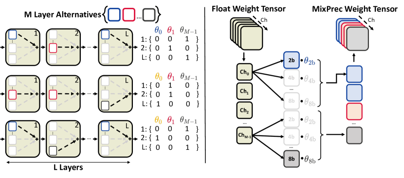
Figure 2: Examples of $\theta$ encoding for Layer Selection (left) and for Mixed-Precision Assignment (right).

A more recent and time-efficient exploration scheme is based upon parametrizing the search space via a set of trainable parameters $\theta$, and optimizing these parameters using gradient descent as a search strategy [24]. Each point of the search space is identified by a specific combination of $\theta$ values. Fig. 2 shows two examples of this parametrization. On the left, arrays of $\theta_{i}$ parameters encode the choice between mutually exclusive layer alternatives. On the right, each $\theta_{i}$ is similarly associated with a specific quantization format (e.g., 2-, 4-, 8-bit) for every channel (or filter) of a convolution’s weights. The main benefit of parametrizing the search space in this way is that we can explore it (i.e., optimize the $\theta$ values) in a standard training loop, jointly with the normal network parameters $W$. This can be achieved either through a continuous relaxation of the sampling followed by a discretization at the end of training [24], or through various forms of differentiable discrete sampling [25]. Regardless of the sampling scheme, these methods commonly train $W$ and $\theta$ to optimize a loss function in the form:

$$\min_{W,\theta}\left[\mathcal{L}_{\text{task}}(W,\theta)+\lambda\mathcal{C}(\theta)\right]$$ (1)

where $\mathcal{C}$ is a differentiable cost estimate that takes into account non-functional metrics, $\mathcal{L}$ is the standard task-specific loss function (e.g., cross-entropy loss), and $\lambda$ is a scalar controlling the trade-off between $\mathcal{C}$ and $\mathcal{L}$. For instance, $\mathcal{C}$ might encode with a differentiable function metrics such as the model size, or the inference latency [26].

This work tackles the problem of DNNs mapping on heterogeneous CUs as a differentiable optimization, performed at training time, following the scheme detailed above. The problem is framed either as layer selection or mixed-precision assignment. These two techniques are generally introduced in Sec. II-B1 and Sec. II-B2, while Sec. IV details how they are applied to the mapping problem studied in this manuscript.

II-B1 Layer Selection

The first and most straightforward application of the differentiable DNN optimization paradigm is layer selection. In this case, the search space is encoded by building a supernet [24] which is a DNN that incorporates multiple alternative paths for each layer, with each path representing a candidate solution. For example, as shown in the left part of Fig. 2, each layer of a reference DNN can be replaced with a module containing various alternatives, such as convolutions with different filter sizes or depthwise vs standard convolutions. During training, the selection of each of these alternatives is associated with trainable parameters $\theta$, optimized according to Eq. 1. After training, a discretization stage selects the best path by combining the alternatives with the highest $\theta$ in each supernet layer. In the literature, this approach is often known as path-based Differentiable Neural Architecture Search (DNAS) [27].

II-B2 Mixed-Precision Assignment

Mixed-precision quantization refers to an optimization in which different parts of a DNN are quantized to different data formats, possibly providing time, memory, and energy savings with respect to fixed-precision solutions, especially when native hardware support for sub-byte operations is available [28, 29, 19, 8]. However, the space of possible bit-widths assignments for different parts of the network is huge and exponential with the depth of the DNN. Thus finding an optimal assignment, e.g., to minimize the latency with a certain accuracy constraint is far from trivial.

Some solutions to this problem use sensitivity-based heuristics [30] or RL [28]. More recently, the differentiable optimization paradigm has been exploited also for this problem [31, 29] where the bit-width assignment is optimized during training by solving an optimization problem of the form of Eq. 1. In this case, as shown in the right part of Fig. 2, the $\theta$ trainable parameters are associated to different versions of the same tensor quantized at different bit widths. Then, an appropriate cost function $\mathcal{C}$ is used to guide the optimization promoting the $\theta$ parameters associated with quantizations that yield a good trade-off between inference cost and accuracy. At the end of the training, the bit-widths that have been assigned the largest $\theta$ coefficient are selected for each tensor.

TABLE I: Summary of state-of-the-art Mapping strategies on Heterogeneous Hardware

Method	Partitioning Engine	Platform	Target Metric	Network Type	Mapping Granularity	Acc. awareness
Wang et al. [10]	Fastest First	CPU+GPU+NPU	Latency/Energy	CNN	Entire Network	✗
HDA [32]	Heuristic	Multiple NPUs	Latency	CNN	Entire Network	Partial
Vasiliadis et al. [11]	RF Scheduler	CPU+GPU	Latency/Energy	CNN	Layer-wise	✗
Tu et al. [12]	Heuristic	GPU+FPGA	Latency/Energy	CNN	Layer-wise	✗
AxoNN [33]	Linear Programming	GPU+NVDLA	Latency/Energy	CNN	Layer-wise	✗
Jeong et al. [13]	Heuristic	GPU+NVDLA	Throughput	CNN	Layer-wise	✗
HaX-CoNN [34]	SAT Solver	GPU+NVDLA	Latency	CNN	Layer-wise	✗
Omniboost [35]	Monte Carlo Tree Search	CPU+GPU	Throughput	CNN	Layer-wise	✗
H3M [36]	Evolutionary	FPGA	Energy-Delay Product	CNN/Transformer	Layer-wise	✗
MaGNAS [37]	Evolutionary	GPU+NVDLA	Latency/Energy	GNN	Layer-wise	✓
AccPar [15]	Dynamic Programming	TPU-v2/v3	Training Latency	CNN	Intra-Layer	✗
Map-and-Conquer [38]	Evolutionary	GPU+NVDLA	Latency/Energy	CNN/Transformer	Intra-Layer	Partial
Ours	Gradient-based	DIANA, Darkside	Latency/Energy	CNN	Intra-Layer	✓

III Related Works

How to efficiently map computationally expensive workloads onto the CUs available on heterogeneous systems represents a compelling problem. Initial studies concentrated on general-purpose workloads, such as OpenCL programs [39]. However, in recent years, there has been a growing interest in the more specific domain of DNN inference. In [10], a mobile SoC composed of CPU, GPU, and NPU is considered. At any time the fastest available CU is selected to map the entire DNN, parallelizing multiple inference requests. Similarly, HDA [32] considers the case of an edge inference server equipped with custom NPUs with 8, 7, and 6-bit quantization. In this case, a scheduling approach is proposed to map entirely and concurrently multiple DNN inference requests to minimize latency. Namely, when a new request arrives, the fastest available NPU that satisfies a certain accuracy threshold is selected. This accuracy threshold is defined task-wise and takes into account the resiliency of the considered DNNs to quantization (profiled offline). [11] explores DNN mapping on CPU and GPU at the granularity of single layers. At runtime, layers are mapped to CUs to minimize the overall inference energy or latency using a Random Forest (RF) predictor, that uses the layer’s hyper-parameters as input features. [12] profiles DNNs execution over a multi-accelerator system including a GPU (NVIDIA Jetson TX2) and an FPGA (Xilinx Artix7), coming up with a heuristic mapping strategy consisting of offloading the whole network to the GPU, except for Fully-Connected (FC) layers which are executed on the FPGA. AxoNN [6] considers partitioning DNNs at the layer level on an NVIDIA Jetson AGX Xavier. Using a linear programming approach, the energy versus latency trade-offs offered by offloading parts of a DNN to the GPU or the NVDLAs are explored. [13] proposes an alternative mapping scheme for the same platform, where the focus is improving throughput by exploiting data parallelism and pipelining among GPU and NVDLAs. HaX-CoNN [34] uses a SAT solver to optimize the latency of the interleaved execution of multiple DNNs, mapped at the layer granularity over the CUs of an NVIDIA Jetson TX2. Similarly, Omniboost [35] proposes an layer-wise mapping scheme based on Monte Carlo Tree Search for serving multi-DNN workloads to minimize throughput on a platform including 2 CPUs and a GPU. H3M [36] targets datacenter FPGAs with an evolutionary-based strategy to map onto the HW multiple DNNs with layer granularity to minimize energy-delay product. MaGNAS [37] explores the per-layer mapping of Graph Neural Networks (GNNs) over GPU and NVDLAs. Concurrently the architecture of the GNN is also optimized. Both mapping and architecture are optimized using an evolutionary algorithm to maximize accuracy on the considered task while reducing the energy or latency.

All these previous works consider coarse mappings where the atomic element that is assigned to a certain CU is an entire layer. Conversely, AccPar [15], explores finer-granularity intra-layer partitions. Taking into account compute performance and communication overheads, dynamic programming is used to optimize DNN training latency over a cluster of multiple Google TPU-v2/v3 accelerators. The considered partitioning axes are: over batches (i.e., data parallelism), input channels, or output channels. Targeting inference, instead, Map-and-Conquer [38] explores intra-layer mappings considering again a Jetson AGX Xavier as the target platform. An evolutionary algorithm is used to explore different partitioning schemes to find the optimal energy-delay product. The intra-layer mapping is achieved at the channel level in Convolutional Neural Networks (CNN) and the head level in Vision Transformers (ViT) by neglecting the data dependencies between contiguous groups of weights. This operation is performed post-training considering the optimization objective defined in [40], originally proposed for pruning, thus the impact on accuracy is only partially taken into account. Moreover, as in MaGNAS [37], the accuracy effect is not related to specific characteristics of the CUs, but only to the architecture of the network.

Conversely, our method considers fine-grained intra-layer mappings aimed at optimizing any cost metric such as energy or latency while being completely accuracy-aware.

We report in Table I a summary of the state-of-the-art mapping schemes on heterogeneous platforms. Importantly, to our knowledge, ours is the first approach in the literature to consider a gradient-descent-based method to optimize the mapping/partitioning of DNN computations onto multiple hardware accelerators.

IV Proposed Method

The majority of the related works discussed in Sec. III are accuracy-unaware, and only explore the trade-off between latency and throughput or latency and energy. Therefore, they do not consider heterogeneous platforms where the execution on different CUs may affect the final task accuracy. This is the case of new edge-oriented platforms such as [7, 8, 9] where due to different data representations or limitations in the accelerable operations (e.g., depthwise vs standard convolution) accuracy can be heavily impacted by mapping choices. For these reasons, existing methods cannot be applied to such new hardware straightforwardly. HDA [32] which is the sole strategy aware of the possible accuracy impact of different CUs, addresses the different problem of serving multiple inference requests concurrently. In contrast, we concentrate on optimizing a single, unbatched inference, which is the common case in extreme-edge devices. Indeed, these devices usually process newly available inputs immediately, often in real-time.

To the best of our knowledge, ODiMO is the first DNN mapping optimization tool explicitly designed for SoCs that include multiple CUs with the aforementioned accuracy-impacting constraints. It optimizes the hyper-parameters of a DNN (e.g., layer type or quantization precision) and its consequent partitioning onto heterogeneous CUs, at training time, optimizing the trade-off between accuracy and energy or latency.

In practice, our method stems from the observation that, for systems including heterogeneous CUs with the incompatibilities described above, optimizing a DNN’s architecture (e.g. layer type or quantization format), and determining its mapping onto the various CUs, reduce to the same problem. In fact, assigning a certain operation or data format to part of the DNN, automatically means that such part will be executed on the specific CU(s) that supports it. Therefore, we can adapt existing gradient-based DNN optimization techniques to address the heterogeneous mapping problem.

Furthermore, while the majority of the other mapping strategies limit the search space to coarse layer-wise mappings (where entire layers are executed on a single CU), ODiMO enables a fine-grain intra-layer partitioning, which increases the utilization of all CUs.

The rest of this section is organized as follows. Sec. IV-A formalizes the network optimization/mapping problem and the proposed ODiMO strategy. Sec. IV-B shows how to use ODiMO to map DNNs onto CUs characterized by incompatible quantization formats, while Sec. IV-C presents the case of mapping onto SoCs with specialized HW units.

IV-A Mapping optimization strategy

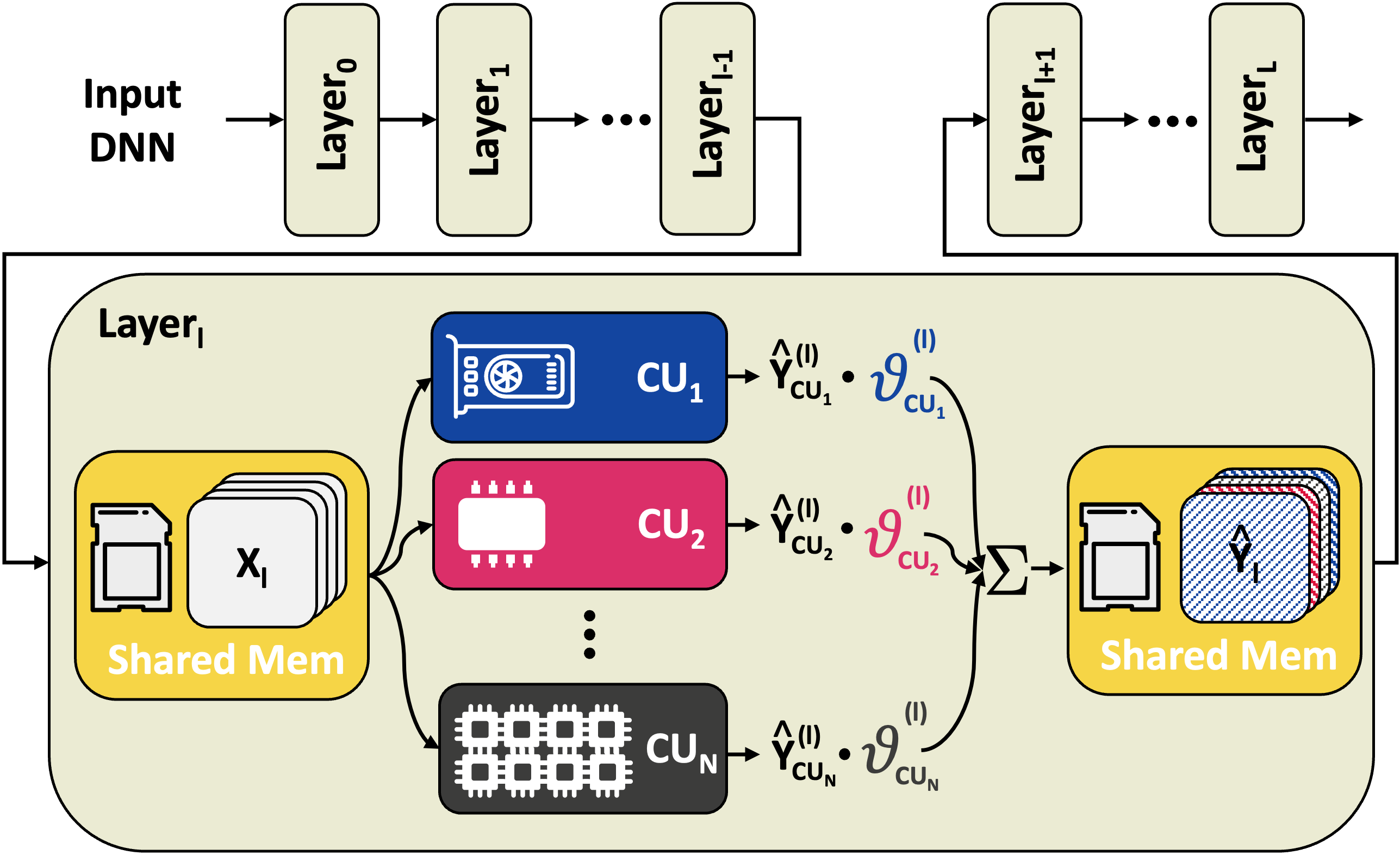
Figure 3: General ODiMO mapping strategy for a layer.

Given a SoC with $N$ different Computing Units (CUs) and a DNN, ODiMO explores how to partition each Convolutional (Conv) or FC layer, at the level of individual output channels/neurons, among the available CUs. In the following discussion, we will always use the term output channels, without loss of generality. Fig. 3 shows an example of the mapping operated by ODiMO for a Conv layer: all accelerators take the entire layer’s input, and produce a subset of the output activations’ channels. As anticipated in Sec. I, we consider heterogeneous systems where all the CUs can access a shared memory region (represented in yellow in Fig. 3) for loading/storing the layer input/partial output. This requirement is met by many different real-world designs such as [15, 8, 7, 9]. Nonetheless, as said before, this work could be easily extended to CUs with private memories by considering the overhead of broadcasting the required input data to them.

Given this fine-grain intra-layer mapping, the size of the search space explodes: e.g., for just $N=2$ CUs and a ResNet18 CNN, there are about $10^{39}$ possible ways to assign each channel of each layer to one of the two units. To efficiently explore a search space of such size, ODiMO adopts a differentiable optimization strategy, where the possible mappings are parametrized through trainable parameters $\theta$.

In this way, by solving an optimization problem similar to the one of Eq. 1 we can efficiently explore mappings while training the DNN, balancing cost and task-accuracy in one-shot. In particular, ODiMO is inspired by recent work on differentiable fine-grained mixed-precision quantization [29] and differentiable layer-selection [24].

As shown in Fig. 3, first, ODiMO identifies the layers $l$ that can be mapped onto the available CUs. Then, it simulates the effect of offloading the computation of every entire layer’s output $\hat{Y}_{i}^{(l)}$ to every CU. The result is a set of $N$ possible outputs $\left\{\hat{Y}_{CU_{j}}^{(l)}\right\}_{j}^{N}$. Finally, the effective output feature map $\hat{Y}^{(l)}$ is built by forming each of the $C_{out}^{(l)}$ output channels as a linear combination of the output produced by each accelerator, weighted by the set of trainable parameters $\theta=\left\{\theta^{(l)}_{CU_{j},\>c}\right\}_{j,\>c}^{N,\>C_{out}^{(l)}}$. In this way, ODiMO builds each layer’s output as a mixture of what would be produced by all available accelerators, given their computing scheme. Mathematically, we compute each output channel $c$ of each layer $l$ as:

$$\hat{Y}^{(l)}_{c}=\sum_{j}^{N}\theta^{(l)}_{c,\text{CU}_{j}}\hat{Y}^{(l)}_{c,\text{CU}_{j}}$$ (2)

The final goal of the ODiMO optimization is to set $\theta^{(l)}_{c,\text{CU}_{j}}=1$ if offloading the $c$-th output channel of the $l$-th layer to the $j$-th CU yields the best accuracy vs energy/latency tradeoff, and $\theta^{(l)}_{c,\text{CU}_{k}}=0$ for all other accelerators with $k\neq j$. During the optimization, the values of $\theta$ can be either sampled discretely [25] or relaxed to assume continuous values in [0,1], e.g., by applying a $\mathrm{softmax}$ operator to a vector of free trainable parameters $\bar{\theta}$ [24]. At the end of the training, the CU whose $\theta_{CU_{j,c}}$ is associated with the largest sampling probability (or value, in the case of a continuous relaxation) is selected as the final offloading target for the $c$-th channel. After the final assignment of channels to accelerators is determined, the layer is reorganized into N parallel sub-layers, each comprising the subset of channels that have been assigned to the $j$-th CU. These $N$ sub-layers can be executed in parallel, and their outputs will be concatenated in the shared memory to be used as inputs for the next layers. More details on this conversion process are provided in Sec. IV-B.

The assignment of channels is optimized by training the DNN, modified as detailed above with the additional $\theta$ parameters, to minimize the loss function of Eq. 1. Namely, the $\theta$ and the normal weights $W$ are trained jointly. In the loss function, the cost term $\mathcal{C}(\theta)$ can change depending on the optimization’s non-functional goal. The formulation can be extended to any cost metric that can be expressed as a differentiable function of $\theta$. For example, when considering latency, the objective of ODiMO is to minimize:

$$\mathcal{C}=\sum_{l}M^{(l)}\mathrm{,\ }M^{(l)}=\max(LAT^{(l)}_{1}(\theta),...,LAT^{(l)}_{n}(\theta))\vspace{-0.2cm}$$ (3)

where each $LAT^{(l)}_{i}(\theta)$ is a differentiable model, parametrized by $\theta$, of the $l$-th layer’s execution latency on the $i$-th CU, as a function of the channels assigned to it. $M^{(l)}$ is the latency of the entire layer, computed with a $\mathrm{max}()$ operation since we assume that all CUs run in parallel. We consider this scenario because minimizing the idleness represents the optimal choice for both time and energy reduction. In practice, since we need a fully-differentiable loss term, we substitute the $\mathrm{max}$ operation of Eq. 3 with its smooth differentiable approximation, computed as the sum of the different terms weighted by the corresponding $\mathrm{softmax}$-ed parameters. For energy reduction, instead, we use the following model:

$$\mathcal{L}_{\mathcal{R}}=\sum_{l}\sum_{i}P_{act,\>i}\cdot LAT^{(l)}_{i}+P_{idle,\>i}\cdot(M^{(l)}-LAT^{(l)}_{i})\vspace{-0.2cm}$$ (4)

The first term of the sum takes into account the energy consumption of the $i$-th CU when it is performing computations, where $P_{act,\>i}$ represents its average active power consumption. The second term represents the energy spent by the $i$-th CU when idle due to waiting for other CUs to finish executing their portions of the considered layer. $P_{idle,\>i}$ is the average idle power consumption.

Regardless of the specific hardware platform considered, ODiMO entails three training phases to generate an optimized mapping. In the first phase (Warmup), the mapping parameters $\theta$ are kept frozen, and the network is trained to minimize the task loss $\mathcal{L}$ only (without considering cost) through the $W$ parameters. Then, we move to the Search phase where cost $\mathcal{C}$ and task loss $\mathcal{L}$ are jointly optimized as in Eq. 1, and both the $\theta$ and the standard weights $W$ are trained, in order to find a well-performing assignment of layer portions to CUs. Finally, during the Final Training phase, the assignment of channels to CUs is frozen based on the values of the $\theta$ parameters at the end of the search, and, similarly to warm up, the $W$ weights are trained for some more epochs to optimize $\mathcal{L}$ alone. This phase allows the model to recover possible accuracy drops due to the final discretization of the mapping.

During the Search phase, the scalar value $\lambda$ of Eq. 1 is used as a knob to control the trade-off between the task loss $\mathcal{L}$ and the cost $\mathcal{C}$. Namely, large values of $\lambda$ will prioritize solutions with a low non-functional cost $\mathcal{C}$, while smaller values will give more importance to the task loss $\mathcal{L}$. Repeating the optimization varying $\lambda$, ODiMO can generate a complete Pareto front in the accuracy versus cost space.

IV-B SoC with Incompatible Data Formats

In this section, we describe a first practical instance of the ODiMO scheme for SoCs with multiple CUs with incompatible quantization. An example of this kind of SoC is represented by DIANA [8] which includes a Digital and an Analog CU with respectively 8bit and ternary precision for the weights. Other examples include the custom variable precision NPUs considered in HDA [32] or the SoC presented in [7], where an NMC CU is coupled with an AIMC one.

In this case, the problem of selecting which CU will execute each layer’s channel can be transformed to a precision assignment problem, similar to the one tackled in [29]. Differently from standard precision assignment, however, in this case, the selected precision does not only influence the model accuracy, but also the inference energy/latency costs, by implicitly limiting the mapping options for that channel to the accelerator(s) supporting the selected precision. For example, in the case of DIANA, assigning ternary precision to the $c$-th channel automatically means that it will be executed on the AIMC CU, with a certain associated cost. Similarly, assigning a channel to 8-bit precision implicitly corresponds to mapping its execution onto the digital CU, with a different impact on latency/energy, and accuracy.

Therefore, with reference to the general ODiMO formulation of Sec. IV-A (Eq. 2), in this case the different CU outputs $\hat{Y}^{(l)}_{c,\text{CU}_{j}}$ represent the results of different versions of the same layer, with weights quantized at different precision. Then, using the 3-phase training scheme discussed above, ODiMO optimizes the assignment of each channel to a given quantization bitwidth, and therefore, to the corresponding CU.

However, one important caveat is that, in the optimization output, the channels assigned to a given CU for each layer are not ordered. For instance, for a layer with $C_{out}^{(l)}$=8 and two CUs, channels 0, 3, and 5 could be assigned to $\text{CU}_{0}$, and channels 1, 2, 4, 6, and 7 to $\text{CU}_{1}$. Deploying the layer as is could lead to an inefficient implementation, as different CU outputs will be interleaved in the shared memory. A more efficient alternative is represented by grouping all channels associated to the same CU in contiguous output locations. Therefore, Fig. 4 shows a layer transformation pass applied to the DNN after the optimization, and before the deployment on the target SoC. We show it for a Conv layer, as an example, representing activation channels side-by-side with squares, and weight filters as “cubes”. The colors used for the shapes’ outlines encode the assignment to a certain accelerator. Color patterns are added to some filters/output slices to clarify the process. The starting point is an ODiMO output, depicted in the top-left part of the figure. We then group the channels in $Y^{(l)}$ and the corresponding filters in $W^{(l)}$ that will be dispatched to the same accelerator. Moreover, the weights of the next layer $W^{(l+1)}$ are also reordered across the input channels dimensions to preserve the network functionality. This process is depicted in the middle part of Fig. 4. Finally, as shown in the right part of Fig. 4, $N$ independent sub-layers, executable in parallel, are obtained by splitting the original one. This step enables the deployment of the obtained mapping onto the $N$ available CUs, without requiring any data-marshaling overhead to aggregate their outputs.

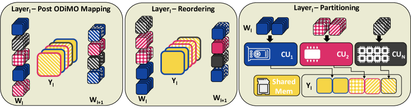
Figure 4: Final layer re-organization pass to support partitioning.

Note that, in the previous part of this section, we presented the case of CUs with incompatible weight quantization formats as a specific case of the general ODiMO mathematical framework (Eq. 2). While this formulation is perfectly valid, our actual implementation is different, purely for training efficiency reasons. Namely, rather than combining the output activations produced by layers with differently quantized weights, we exploit the linearity of Conv/FC operations to directly combine the weights. Namely, we exploit the following factorization, equivalent to Eq. 2:

$$\hat{Y}^{(l)}_{c}=(\sum_{j}^{N}\theta^{(l)}_{c,\text{CU}_{j}}W^{(l)}_{c,\text{CU}_{j}})*X^{(l)}$$ (5)

where $W^{(l)}_{c,\text{CU}_{j}}$ is the c-th weights kernel of the l-th layer, quantized at the precision supported by the j-th CU. The part inside parentheses represents an effective weights filter. The advantage of this alternative formulation is that it does not require computing multiple separate convolutions for each layer. Rather, it just requires constructing the effective weights, through simpler element-wise operations. Therefore, it reduces the execution time of ODiMO.

IV-C SoC with Specialized HW Units

This section presents how to tailor ODiMO to CUs that are compatible from the data format standpoint, but support the execution of different types of layers. This is the case of SoCs such as Darkside [9] where a general-purpose multi-core cluster of RISC-V processors is coupled with an accelerator specialized to efficiently execute depthwise convolutions, the DepthWise Engine (DWE). Another example that fits this scheme is Kraken [41], a RISC-V heterogenous SoC that includes a multicore cluster, and a Sparse Neural Engine to execute event-based spiking DNNs. Usually, layers such as normal and DW Convolutions are alternated sequentially, leading to a situation in which only one CU is used at any time. Exploiting the ODiMO optimization framework, we can instead execute multiple sub-layers in parallel, e.g., one normal Conv and one DW, each with fewer output channels. The fraction of channels produced by each sub-layer can be optimized with ODiMO, considering both the relative speeds (or energy consumptions) of the CUs, and the impact of each type of layer on accuracy. As for the case of quantization, executing standard and DW Convs in parallel exposes an interesting trade-off, i.e., a DW Conv will encompass much fewer OPs with respect to a standard one but it will probably impact accuracy more.

More formally, we use once again the scheme of Eq. 2, where this time, $Y^{(l)}_{c,\text{CU}_{j}}$ and $Y^{(l)}_{c,\text{CU}_{k}}$ with $k\neq j$ represent two (possibly different) tensor operations, as supported by each CU. While this scheme can in general accommodate different types of layers (e.g., convolutions with different filter sizes), we test it in practice for the combination of normal and DW convolutions.

Also in this case, the raw ODiMO output has to be slightly altered to produce practically usable DNNs. Namely, we need once again to assign consecutive channels to the same CU. In general, if we map the first $n_{c}$ channels to the DW conv, then the trailing $C_{out}-n_{c}$ channels should be executed as a normal convolution. As for the quantization case, this constraint is needed to avoid costly data marshaling operations during the actual execution of the workload on the SoC. However, differently from what is discussed in Sec. IV-B, such “grouping” cannot be achieved through a post-optimization step. In fact, due to the constraints of DW layers (each output channel being a function of just one input channel), the presence of two or more consecutive layers of this kind, each enforcing a different reordering, would make a transformation like the one of Fig. 4 impossible. Instead, we can enforce the generation of an output with all channels assigned to the same CU “grouped”, by constraining the optimization process. Namely, rather than generating the $\theta$ array of each layer just by soft-maxing independent elements, we further combine the array elements as follows:

$$\theta^{(l)}_{i}=\sum_{j=1}^{N-i}\hat{\theta}^{(l)}_{N-j}$$ (6)

This formulation enforces that if $i>j$, then $\theta^{(l)}_{i}\leq\theta^{(l)}_{j}$. This, in turn ensures that the channels mapped to the same CU are always contiguous. Despite this additional constraint in the optimization, as shown in Sec. V, ODiMO is still able to discover Pareto-optimal mappings that exploit the HW better than manual mappings.

V Experimental Results

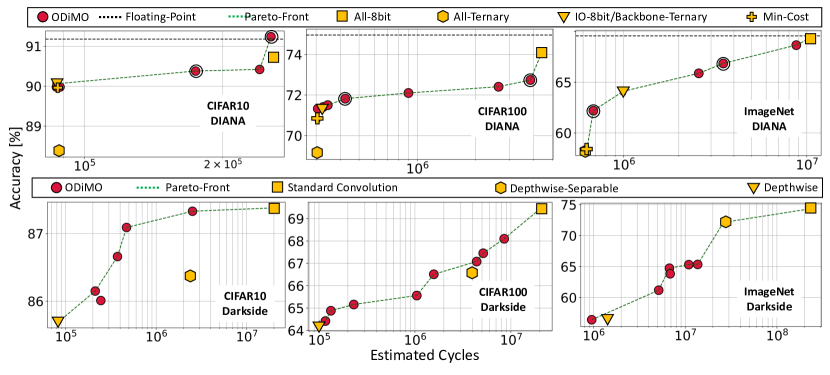
Figure 5: Mappings obtained using ODiMO with latency as optimization target.

V-A Setup

We benchmark ODiMO on three edge-relevant image classification datasets: i) CIFAR-10 [42]; ii) CIFAR-100 [42]; iii) ImageNet-1k [43]. We target two different platforms, namely Diana [8] and Darkside [9] as examples of SoCs including CUs with incompatible data formats (case of Sec. IV-B) and supporting different layer types (Sec. IV-C), respectively.

One key element of our methodology that changes for different hardware targets is the expression of the cost term $\mathcal{C}$ in the optimization objective (Eq. 1). Moreover, the details of the 3-phase training protocol described in Sec. IV-A, also need to be slightly modified depending on the target. For details on both these platform-specific customizations, we refer the readers to Appendix A.

For each dataset, we use as blueprint for our optimization DNNs well-suited to be mapped either on DIANA or on Darkside. We choose MobileNetV1 [20] for Darkside, for all three benchmarks, to properly exploit the depthwise engine. Starting from the original MobileNet architecture, we let ODiMO optimize a supernet that includes two alternatives (normal Conv and DW Conv) for each layer that has $C_{out}=C_{in}$. Conversely, for the DIANA platform, which is not optimized to execute depthwise layers (depthwise convolutions can only be executed on the digital CU, and with lower efficiency w.r.t. standard conv), we adopted networks of the ResNet [44] family. In particular, we employed a ResNet20 for CIFAR-10 and a ResNet18 for both CIFAR-100 and ImageNet. ODiMO is implemented in Python 3.10 and PyTorch v2.3, extending the PLiNIO [27] DNN optimization library.

We compare ODiMO with several baseline mapping alternatives depending on the considered HW. On DIANA, we consider the following baselines: i) All-8bit and All-Ternary, which are simple mappings utilizing exclusively the digital and AIMC accelerators, respectively; ii) IO-8bit/Backbone Ternary, a heuristic method proposed in [8] that assigns the first and last layers to the 8-bit accelerator and the intermediate layers to the AIMC accelerator, based on the general guideline that aggressively quantizing the layers near the input and output can significantly impair accuracy; iii) Min-Cost, an optimized deterministic mapping that employs the same channel-wise partitioning as ODiMO, aiming solely at minimizing cost, without considering accuracy. Specifically, it statically assigns the channels of each layer to the AIMC and digital accelerators before training, intending to minimize Eq.3 or Eq.4. If multiple solutions yield equivalent costs, digital channels are maximized as this is expected to enhance accuracy.

On Darkside, we consider three baselines. The first is the standard MobileNet with Depthwise-Separable convolutions, i.e., alternations of DW and pointwise convolutions (standard Conv with 1x1 filters). Then, we consider the case of layers entirely mapped either on the cluster or on the DWE. When the entirety of the network is mapped on the cluster we always execute $3\times 3$ standard convolution in place of the original Depthwise-Separable, while in the case of the DWE, a $3\times 3$ DW convolution is used. Additionally, we apply our optimization to MobileNets initialized with different width multipliers.

V-B Training Hyper-Parameters

For each of the three tasks, we use different training hyper-parameters. We report the main choices here for reproducibility, referring the reader to our open-source code for the remaining details.

We set the training epochs for the warmup, search, and fine-tuning phases to 500, 200, and 130 for the CIFAR-10, CIFAR-100, and ImageNet benchmarks, respectively. We apply early-stopping using as control metric the validation accuracy with patience equal respectively to 50, 100, and 30 epochs for CIFAR-10, CIFAR-100, and ImageNet. For each benchmark, the standard cross-entropy loss is used as task loss $\mathcal{L}$.

On DIANA, we use the SGD optimizer for the weights $W$, with a learning rate of 1e-2, a momentum of 0.9, and a weight-decay of 1e-4. Instead, for the $\theta$ parameters, we use the Adam optimizer with a learning rate of 1e-3. On Darkside, we use the Adam optimizer for both kinds of optimization parameters with a learning rate of 1e-3 for CIFAR-10 and CIFAR-100 and of 1e-4 for ImageNet.

V-C Search-Space Exploration

V-C1 Latency Optimization

Fig. 5 presents the results obtained with ODiMO on the three benchmarks in the accuracy versus estimated latency for DIANA (top row) and Darkside (bottom row), with latency estimated using the cost models described in Appendix A. All the reported accuracies are on the test set with Pareto points selected on the validation set. Each ODiMO point is obtained varying the regularization strength $\lambda$ of Eq. 1. We also report the baselines discussed in Sec. V-A in green and the floating point DNN accuracy as a horizontal dashed line.

In all graphs, the majority of the ODiMO points either dominate the baselines or are part of the Pareto frontier. This demonstrates the effectiveness of our approach. Importantly, ODiMO produces a rich set of intermediate Pareto-optimal mappings, achieving intermediate accuracy vs latency-tradeoffs in-between the various baselines, that could not be obtained otherwise.

On DIANA, ODiMO can trade-off the estimated latency and accuracy with respect to the All-8bit baseline on CIFAR-10 (3rd red dot from the right in the top-left graph) achieving a $1.48\times$ speedup with an accuracy drop lower than $0.5\%$. Moreover, it also discovers a mapping (1st red dot from the right) that matches the floating-point accuracy, thus improving by +$0.5\%$ the accuracy of All-8bit, thanks to the regularizing effect of ternarization. On CIFAR-100, our tool discovers solutions spanning more than one order of magnitude on the x-axis, that can offer a speed-up of $1.15\times$ and $4.9\times$ for an accuracy drop $<$$1.5\%$ and $<$$2\%$ w.r.t. the 8bit baseline, respectively (1st and 3rd red dot from the right, top-middle figure). When comparing to the min-cost baseline, we can achieve a $0.5\%$ improvement in accuracy at iso-cycles. Also on the ImageNet task, ODiMO is able to obtain a collection of Pareto points spanning more than one order of magnitude of estimated cycles. In particular, w.r.t. All-8bit we improve the latency by up-to $1.2\times$ and $3\times$ for a drop of $<$$1\%$ and $<$$2.5\%$ accuracy (1st and 2nd red points from the right). Moreover, at the cost of $1.08\times$ more cycles, we are able to improve by +$3.8\%$ the Min-Cost accuracy (leftmost red point).

The bottom row of Fig. 5 shows the results obtained targeting the Darkside platform. On the CIFAR-10 benchmark (bottom-left figure) we reduce latency by up to $8\times$ while being as accurate as the standard convolution baseline (rightmost red point in the bottom-left plot). Instead, when comparing with the Depthwise-Separable baseline (i.e., vanilla MBV1) we can improve accuracy by +$0.7\%$ while also offering a $4.98\times$ speed-up (2nd red point from the right). On CIFAR-100, ODiMO offers Pareto optimal points spanning two orders of magnitude in latency. Noteworthy, with an accuracy drop respectively of -$1.5\%$ and -$0.1\%$ we achieve in both cases a speed-up of $2.4\times$ when comparing to standard and depthwise-separable convolutions respectively (1st and 4th red points from the right in the bottom-middle plot). Finally, the rightmost plot in the bottom row of Fig. 5 shows the mappings obtained using ODiMO for Darkside on the ImageNet task. In this case, we limit the search space between the Depthwise and the Depthwise-Separable baselines as corner mappings. To do this, we consider as layer alternatives either DW or DW-Separable (DW + Pointwise) Convolutions, as opposed to DW versus normal Conv. We opted for this choice because, in our preliminary experiments, we discovered that when considering the whole search space the discovered mappings would collapse either on the Depthwise or the Standard Convolution baselines. Also on this challenging task, we are able to obtain Pareto-optimal mappings. Noteworthy, we can reduce the number of cycles by $1.49\times$ while improving accuracy by $0.2\%$ compared to the Depthwise baseline (leftmost red point). In the higher accuracy range, the drop with respect to the Depthwise-Separable baseline is 6.8%, which is traded for a cycles reduction of 2.5$\times$.

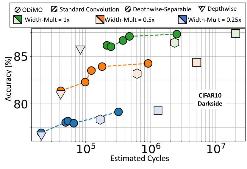
Figure 6: Mappings obtained using ODiMO with latency as optimization target and different width multiplier.

In Fig. 6 we show the mapping obtained using ODiMO with the Darkside latency model, on the CIFAR-10 task, using the same MBV1 net with three different width-multipliers. Namely, we consider $1\times$ (i.e., the same DNN as in Fig. 5), $0.5\times$, i.e., with half of the original channels and $0.25\times$, i.e., with a quarter of the original channels. In all these three variants we always obtain a rich collection of Pareto-optimal mappings. This demonstrates how ODiMO is effective regardless of the number of channels, which is the geometric dimension of the convolution operation used to perform the partitioning over the different CUs. Moreover, we can notice how the mappings discovered with a width-multiplier of $1\times$ (green curve) always Pareto dominate the solutions obtained with smaller width multipliers (including the baselines). This is due to the high efficiency of the DWE accelerator, which can compute a high number of DW output channels with low latency. For instance, when comparing vanilla MBV1 with half/quarter of the original channels we are able to improve accuracy by up to $4\%$ and $6.7\%$ at iso-latency. This experiment demonstrates how partitioning the execution of each DNN layer over heterogeneous computing units with fine-grained mappings can be a way to reduce latency without incurring the accuracy drop associated with channel pruning.

V-C2 Energy Consumption Optimization

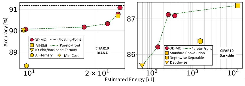
Figure 7: Mappings obtained using ODiMO with energy as optimization target.

To demonstrate the generality of ODiMO to the specific non-functional cost metric we built an energy cost model in the form of Eq. 4 for both DIANA and Darkside. Fig. 7 depicts the results obtained with ODiMO on the CIFAR-10 task. For both hardware platforms, also in this case we obtain Pareto-optimal mappings effectively balancing energy consumption and accuracy. In particular, in the leftmost plot, we present the results obtained with DIANA. Noteworthy, when accepting an accuracy drop of -$0.37\%$ we can reduce the energy by $1.41\times$ compared to the All-8bit baseline. Instead, with the Darkside energy model (rightmost plot), with an accuracy drop of -$0.26\%$ and -$0.15\%$ we can improve the energy efficiency by $50.8\times$ and $11\times$ when comparing respectively with the Standard and Depthwise Convolution baselines. When comparing to the Depthwise-Separable baseline, i.e., the vanilla MobileNet, ODiMO discovered a $6.11\times$ more energy efficient mapping while improving accuracy by $0.76\%$.

V-D Embedded Deployment

This section validates the solutions presented in Sec. V-C. We first validate the DIANA and Darkside hardware models with a micro-benchmarking procedure on selected layers. Then, we present the deployment of a subset of the DNNs found by ODiMO on the DIANA SoC. Please note, that while we were able to perform the micro-benchmarking on Darkside, using numbers reported in the paper [9] as ground truth reference, we do not have the possibility of deploying entire networks on it because the physical HW is not available.

V-D1 Hardware Models Micro-Benchmarking

TABLE II: Micro-benchmarking of DIANA and Darkside HW models on ResNet and MobileNet layers.

	CU	Error	Pearson	Spearman
DIANA	Digital	42%	88%	95%
	Analog	37%	79%	94%
Darkside	DWE	9%	99.9%	99.8%
	Cluster	18%	95%	89%

In this section, we validate the four analytical HW models detailed in Appendix A, respectively for DIANA and Darkside. In particular, we compare the number of predicted cycles against the ones measured on the actual SoCs for the same DNN workloads. The different workloads refer to layers taken from ResNet and MobileNet architectures respectively, with different geometries. For each model, we computed the Pearson and the Spearman correlation coefficients which measure respectively the strength of the linear relationship and the rank monotonicity between the modeled and real cycles. Moreover, we also computed the average absolute percentage error between the real and the modeled number of cycles. Table II summarizes the results obtained with the four models. Although some models exhibit relatively high average errors, they demonstrate strong correlations with actual measurements, as indicated by a Spearman coefficient consistently above 89%.

V-D2 DIANA Deployment

This section examines the deployment of a subset of the solutions from Fig. 5 on the DIANA SoC, operating at a frequency of 260 MHz, replacing modeled latency and energy with measured values. For each benchmark, we deploy the All-8bit and Min-Cost baselines along with a selection of ODiMO results (indicated by a black circle in Fig. 5). Specifically, we select two points from the Pareto front (Accurate and Fast) for all benchmarks. Each entry of Table III represents a deployed DNNs for which we report accuracy, latency, energy consumption, the percentage of time each CU is utilized during a complete inference (D./A. util.), and the percentage of channels executed on the AIMC CU, i.e., the fraction $\nicefrac{{C_{out}^{aimc}}}{{C_{out}}}$ for the whole DNN (A. Ch.).

TABLE III: Deployment on DIANA of selected solutions from Fig. 5

	Network	Acc.	lat. [ms]	E. [uJ]	D./A. util.	A. Ch.
CIFAR10	All-8bit	90.70	1.55	38.70	100% / 0%	0%
	ODiMO Accurate	91.24	1.55	42.50	100% / 18.6%	5.4%
	ODiMO Fast	90.38	1.07	34.44	100% / 44.8%	51.8%
	Min Cost	90.06	0.47	13.6	9.5% / 93.6%	97.5%
CIFAR100	All-8bit	74.10	30.3	756	100% / 0%	0%
	ODiMO Accurate	72.74	26.2	669	100% / 7.3%	15%
	ODiMO Fast	71.82	2.14	65.9	70% / 58%	96%
	Min Cost	70.86	1.62	47.6	34% / 77.3%	96%
ImageNet	All-8bit	69.33	63.2	1578	100% / 0%	0%
	ODiMO Accurate	66.85	33.4	881	94% / 31%	59%
	ODiMO Fast	62.19	4.6	136	27% / 87%	97%
	Min Cost	58.38	4.25	129	35% / 86%	95%

On CIFAR10, ODiMO-Fast reduces latency by $1.45\times$ w.r.t All-8bit, for a limited accuracy drop (-$0.32\%$). This result validates the $1.48\times$ reduction estimated with the analytical model (ref Sec. V-C). The reduction is achieved by offloading roughly half of the channels to the analog accelerator. Further, the digital CU is always active while the AIMC CU is active for $44.8\%$ of the inference time. ODiMO Accurate improves the accuracy of the All-8bit baseline by $0.54\%$ by assigning a small fraction ($5.4\%$) of channels to the analog CU, which probably enforces a regularizing effect. Moreover, we can appreciate how the ranking of different mappings discovered by ODiMO (i.e., using the analytical models) is preserved in the deployment on the real HW. Indeed, the $1.45\times$ speed-up of ODiMO-Fast w.r.t. ODiMO-Accurate is well-tracked by the DIANA’s models, which predict a $1.46\times$ speed-up.

On CIFAR100, ODiMO-Fast reduces latency/energy by $14.2\times$/$11.5\times$ with an accuracy drop $<2.5\%$ w.r.t. All-8bit. On the other hand, ODiMO Accurate limits the accuracy drop to $1.36\%$ while being $1.16\times$ faster and $1.13\times$ more energy efficient. When comparing ODiMO Fast with the Min Cost baseline, we achieve 0.96% improved accuracy with a latency/energy overhead of $24.2\%$/$27.8\%$. The fraction of channels assigned to the analog CU is similar for the two mappings (i.e., $96\%$). However, the specific channels assigned to it in different layers change. The accuracy improvement is imputable to this difference, which also causes a higher median usage (+$26\%$) of the digital CU.

On the ImageNet dataset, w.r.t. All-8bit the ODiMO Accurate solution improves latency/energy by $1.89\times$/$1.79\times$ with an accuracy drop $<2.48\%$. This is achieved by offloading $59\%$ of the channels to the analog CU. ODiMO Fast improves the accuracy of Min Cost by $3.81\%$ while being only $1.08\times$/$1.05\times$ slower/less energy efficient. As in the case of CIFAR100, this is achieved by assigning different channels to the digital CU w.r.t. the ones selected by the Min Cost heuristic (which is accuracy unaware). Moreover, the latency penalty of such channel assignments to the digital CU is mitigated by an overall higher number of channels assigned to the analog CU ($97\%$ vs $95\%$). This stresses the importance of a fine-grained mapping methodology, as the one proposed in this work, which is both accuracy- and hardware-aware.

VI Conclusion

We have introduced ODiMO, a tool that partitions a DNN execution at fine grain among multiple accelerators with incompatible quantization formats or implementing different layer alternatives. To do so, it formulates the problem as a cost-aware differentiable optimization addressed simultaneously with the training of DNN weights. With results on different benchmarks and DNN architectures, we have shown that ODiMO can obtain rich Pareto-fronts in both the accuracy vs energy or latency spaces and reduce latency/energy by up to $8\times$/$50.8\times$ with limited accuracy drops compared to single-accelerator solutions or heuristic mappings.

Matteo Risso received his B.Sc degree in Physical Engineering and M.Sc degree in Electronic Engineering at the Politecnico di Torino, Italy, in 2018 and 2020. He is currently working toward his Ph.D. degree at Politecnico di Torino, Italy. His research interests include Embedded Machine Learning and Energy-Efficient Embedded Systems.

Alessio Burrello received his B.Sc and M.Sc degree in Electronic Engineering at the Politecnico of Turin, Italy, in 2016 and 2018. He is currently working toward his Ph.D. degree at the Department of Electrical, Electronic and Information Technologies Engineering (DEI) of the University of Bologna, Italy. His research interests include parallel programming models for embedded systems, machine and deep learning, hardware oriented deep learning, and code optimization for multi-core systems.

Daniele Jahier Pagliari received the M.Sc. and Ph.D. degrees in computer engineering from the Politecnico di Torino, Turin, Italy, in 2014 and 2018, respectively. He is currently an Assistant Professor with the Politecnico di Torino. His research interests are in the computer-aided design and optimization of digital circuits and systems, with a particular focus on energy-efficiency aspects and on emerging applications, such as machine learning at the edge.

Appendix A Real SoC Case Studies

In this appendix, we detail the implementation aspects of our proposed method for the two considered hardware targets, DIANA [8] and Darkside [9]. As discussed in the main part of the manuscript, these two platforms represent respectively an example of SoC that includes CUs with incompatible data formats (Sec. IV-B) and one that includes CUs with specialized HW units (Sec. IV-C). Therefore, through these two examples, this appendix also provides a guide on how ODiMO can be adapted to other similar targets. For each of the two platforms, we detail the analytical latency models that we use as part of our training-time mapping optimization (Sec. A-A1 and Sec. A-B1) and then discuss how we customized the general ODiMO training protocol (Sec. A-A2 and Sec. A-B2).

Latency modeling has been studied extensively in recent NAS literature. A common approach [26] uses a small NN model trained on many profiled layers to predict latency based on the layer geometry. Although this method is compatible with ODiMO, given the high predictability of our considered CUs’ execution, we found that using simpler analytical models that account for the respective parallelism and dataflow yields good-enough results while making the optimization faster.

A-A DIANA

A-A1 DIANA Hardware Models

The DIANA latency models take into account the cycles required for loading inputs, executing GEMMs/Convolutions (accounting for each CU’s parallelism dimension and unrolling factor), and storing outputs. Non-idealities such as programming overheads and memory stalls are ignored. Nonetheless, as experimentally shown in Sec. V-D1 they can exhibit good correlation with actual latencies measured on the hardware. Considering a Convolutional layer, without loss of generality, the latency model for the digital accelerator is:

$$LAT_{dig}^{(l)}(\theta)= \lceil\frac{C_{out,dig}^{(l)}(\theta)}{16}\rceil\lceil\frac{o_{y}^{(l)}}{16}\rceil\times C_{in}^{(l)}\times o_{x}^{(l)}\times f_{x}^{(l)}\times f_{y}^{(l)}+$$

$$C_{in}^{(l)}\times C_{out,dig}^{(l)}(\theta)\times f_{x}^{(l)}\times f_{y}^{(l)}$$

where $C_{in}^{(l)}$, $o_{x}^{(l)}$/$o_{y}^{(l)}$ and $f_{x}^{(l)}$/$f_{y}^{(l)}$ are the layer’s input channels, output spatial dimensions, and kernel sizes respectively. $C_{out,dig}^{(l)}$ is the number of output channels assigned by ODiMO to the digital CU (as a function of the learned $\theta$ parameters). The two addends in the latency model simply compute the number of MAC and DMA cycles respectively, where the former considers the spatial parallelism of the accelerator (16x16 PEs). The model for the AIMC CU is:

$$LAT_{aimc}^{(l)}(\theta)= \lceil\frac{C_{in}^{(l)}\times f_{x}^{(l)}\times f_{y}^{(l)}}{1152}\rceil\lceil\frac{C_{out,aimc}^{(l)}(\theta)}{512}\rceil\times o_{x}^{(l)}\times o_{y}^{(l)}$$

$$+2\times 4\times C_{in}^{(l)}\times\lceil\frac{C_{out,aimc}^{(l)}(\theta)}{512}\rceil$$

also in this case the first term models the number of MAC operations as function of the CU’s parallelism (1152$\times$512) and the second one accounts for DMA cycles.

A-A2 Training Protocol

In this section, we detail how the general training protocol introduced in Sec. IV-A is customized for the case of DIANA. The Warmup consists of training the given DNN in floating-point. Then, since the DIANA accelerators do not implement Batch Normalization (BN) in hardware, the BN layers are folded with Conv/FC. To simulate the effect of quantization during the optimization, we follow the scheme of [45]:

$$Q(x)=\frac{e^{s}}{2^{n-1}-1}\cdot\mathrm{round}(2^{n-1}-1\cdot\mathrm{clip}(x,-1,1))\vspace{-0.1cm}$$ (7)

where $s$ is a trainable scale parameter and $n$ is the bit-width. With reference to Eq. 7, we use $n=8$ for the digital accelerator weights, while $n=2$ is used to perform ternarization i.e., the quantization format of DIANA’s AIMC accelerator weights. Concerning activations, the AIMC and digital blocks have slightly different formats on 7- and 8-bit respectively. During the optimization phase, we use the worst case of the two (7-bit) as fake-quantization bit-width for layers’ inputs/outputs. As long as the DNN is appropriately fine-tuned (see below), we found this approximation not to degrade our results.

During the Search phase, the fake-quantized DNN is optimized until convergence, with an early-stop mechanism. Then, after discretizing the final channel assignment to each CU, the model undergoes the final Final Training step. In this phase, we use the exact quantization format also for activations, i.e., shared data are stored on 8-bit but the AIMC accelerator D/A and A/D converters are on 7-bit, effectively truncating the LSB of inputs/outputs.

A-B Darkside

A-B1 Darkside Hardware Models

Darkside includes a cluster of eight SIMD-enabled general-purpose RISC-V cores coupled with an HW accelerator, the DWE, to execute Depthwise Convolutions with high arithmetic intensity. The latency model of the DWE is defined as:

$$LAT_{DWE}^{(l)}(\theta)= \lfloor\frac{C_{out,DWE}^{(l)}(\theta)+15}{16}\rfloor\times(o_{x}o_{y}\tau_{\text{comp}}+o_{x}\tau_{i}+\tau_{w})$$

where $C_{out,DWE}^{(l)}=C_{in,DWE}^{(l)}$ denotes the number of output/input channels of the layer. $\tau_{\text{comp}},\tau_{i},\tau_{w}$ are constants set respectively to $4,9,$ and $9$ that take into account the number of cycles necessary to compute the fraction of the output pixels corresponding to the loaded input, load a new input portion and load the necessary weights.

Conversely, the model for the RISC-V cluster is derived by analyzing the software routine that implements Conv layers, described in [46]. The model is:

$$LAT_{\text{clust}}^{(l)}(\theta)= \lfloor\frac{o_{y}^{(l)}+1}{2}\rfloor\lfloor\frac{o_{x}^{(l)}+7}{8}\rfloor\times($$

$$2f_{x}^{(l)}f_{y}^{(l)}C_{in}^{(l)}+$$

$$\lfloor\frac{C_{out,clust}^{(l)}(\theta)+3}{4}\rfloor(15+14\lfloor\frac{f_{x}^{(l)}f_{y}^{(l)}C_{in}^{(l)}+3}{4}\rfloor))$$

where the two addends within round brackets take into account respectively the cycles required to perform the so-called im2col transformation, and the cycles spent doing matrix multiplications. The term multiplied by this sum is the number of iterations required to produce the complete output feature map, which accounts for the parallelization over the eight cores, performed on the ox dimension, and for the inner loop unrolling (with a factor of 2) over oy.

A-B2 Training Protocol

The SuperNet used by ODiMO to optimize the layer selection for Darkside includes a normal Conv and a DW Conv as alternatives for each layer, matching the cluster and DWE CUs respectively. Before Warmup, the weights of both alternatives are randomly initialized. To ensure that all paths of the supernet are properly trained, in each iteration of the Warmup phase, we uniformly sample a random number of channels from each of the two alternatives, independently for every layer.

During the Search phase, to avoid the fast convergence of the optimization algorithm towards solutions with low cost but degraded performance, we found it beneficial to implement a strength-scheduling approach, similar to the one proposed in [25], where the target value of the regularization strength $\lambda$ is divided by $100$ and linearly increased over the epochs until the original value is reached, then it is kept constant.

At the end of the search phase, the mapping is discretized and the final discovered network is trained from-scratch by optimizing only the task loss $\mathcal{L}$ with respect to the weights $W$. Differently for DIANA, where fine-tuning was sufficient, in this case, we foundwthat training from scratch is beneficial.

References

- [1] Z. Zhou, X. Chen, E. Li, L. Zeng, K. Luo, and J. Zhang, “Edge Intelligence: Paving the Last Mile of Artificial Intelligence With Edge Computing,” Proceedings of the IEEE, vol. 107, no. 8, pp. 1738–1762, 2019.
- [2] V. Sze, Y.-H. Chen, T.-J. Yang, and J. S. Emer, “Efficient processing of deep neural networks,” Synthesis Lectures on Computer Architecture, vol. 15, no. 2, pp. 1–341, 2020.
- [3] B. Jacob et al., “Quantization and Training of Neural Networks for Efficient Integer-Arithmetic-Only Inference,” in Proceedings of the IEEE Conference on Computer Vision and Pattern Recognition (CVPR). IEEE, 2018.
- [4] M. Risso, A. Burrello, F. Conti, L. Lamberti, Y. Chen, L. Benini, E. Macii, M. Poncino, and D. J. Pagliari, “Lightweight neural architecture search for temporal convolutional networks at the edge,” IEEE Transactions on Computers, vol. 72, no. 3, pp. 744–758, 2023.
- [5] K. Seshadri, B. Akin, J. Laudon, R. Narayanaswami, and A. Yazdanbakhsh, “An evaluation of edge tpu accelerators for convolutional neural networks,” 2021.
- [6] I. Dagli, A. Cieslewicz, J. McClurg, and M. E. Belviranli, “Axonn: Energy-aware execution of neural network inference on multi-accelerator heterogeneous socs,” in Proceedings of the 59th ACM/IEEE Design Automation Conference, ser. DAC ’22. New York, NY, USA: Association for Computing Machinery, 2022, p. 1069–1074.
- [7] H. Jia, H. Valavi, Y. Tang, J. Zhang, and N. Verma, “A programmable heterogeneous microprocessor based on bit-scalable in-memory computing,” IEEE Journal of Solid-State Circuits, vol. 55, no. 9, pp. 2609–2621, 2020.
- [8] K. Ueyoshi, I. A. Papistas, P. Houshmand, G. M. Sarda, V. Jain, M. Shi, Q. Zheng, S. Giraldo, P. Vrancx, J. Doevenspeck et al., “Diana: An end-to-end energy-efficient digital and analog hybrid neural network soc,” in 2022 IEEE International Solid-State Circuits Conference (ISSCC), vol. 65. IEEE, 2022, pp. 1–3.
- [9] A. Garofalo, Y. Tortorella, M. Perotti, L. Valente, A. Nadalini, L. Benini, D. Rossi, and F. Conti, “Darkside: A heterogeneous risc-v compute cluster for extreme-edge on-chip dnn inference and training,” IEEE Open Journal of the Solid-State Circuits Society, vol. 2, pp. 231–243, 2022.
- [10] S. Wang, A. Pathania, and T. Mitra, “Neural network inference on mobile socs,” IEEE Design & Test, vol. 37, no. 5, pp. 50–57, 2020.
- [11] G. Vasiliadis, R. Tsirbas, and S. Ioannidis, “The best of many worlds: Scheduling machine learning inference on cpu-gpu integrated architectures,” in 2022 IEEE International Parallel and Distributed Processing Symposium Workshops (IPDPSW), 2022, pp. 55–64.
- [12] Y. Tu, S. Sadiq, Y. Tao, M.-L. Shyu, and S.-C. Chen, “A power efficient neural network implementation on heterogeneous fpga and gpu devices,” in 2019 IEEE 20th International Conference on Information Reuse and Integration for Data Science (IRI), 2019, pp. 193–199.
- [13] E. Jeong, J. Kim, S. Tan, J. Lee, and S. Ha, “Deep learning inference parallelization on heterogeneous processors with tensorrt,” IEEE Embedded Systems Letters, vol. 14, no. 1, pp. 15–18, 2022.
- [14] Y. Kang, J. Hauswald, C. Gao, A. Rovinski, T. Mudge, J. Mars, and L. Tang, “Neurosurgeon: Collaborative Intelligence Between the Cloud and Mobile Edge,” in Proceedings of the Twenty-Second International Conference on Architectural Support for Programming Languages and Operating Systems. New York, NY, USA: ACM, 2017, pp. 615–629.
- [15] L. Song, F. Chen, Y. Zhuo, X. Qian, H. Li, and Y. Chen, “AccPar: Tensor Partitioning for Heterogeneous Deep Learning Accelerators,” in 2020 IEEE International Symposium on High Performance Computer Architecture (HPCA), Feb. 2020, pp. 342–355.
- [16] L. Zheng, Z. Li, H. Zhang, Y. Zhuang, Z. Chen, Y. Huang, Y. Wang, Y. Xu, D. Zhuo, E. P. Xing et al., “Alpa: Automating inter-and Intra-Operator parallelism for distributed deep learning,” in 16th USENIX Symposium on Operating Systems Design and Implementation (OSDI 22), 2022, pp. 559–578.
- [17] M. Risso, A. Burrello, G. M. Sarda, L. Benini, E. Macii, M. Poncino, M. Verhelst, and D. J. Pagliari, “Precision-aware latency and energy balancing on multi-accelerator platforms for dnn inference,” in 2023 IEEE/ACM International Symposium on Low Power Electronics and Design (ISLPED), 2023, pp. 1–6.
- [18] A. Reuther, P. Michaleas, M. Jones, V. Gadepally, S. Samsi, and J. Kepner, “AI Accelerator Survey and Trends,” in 2021 IEEE High Performance Extreme Computing Conference (HPEC), Sep. 2021, pp. 1–9.
- [19] A. S. Prasad, L. Benini, and F. Conti, “Specialization meets flexibility: a heterogeneous architecture for high-efficiency, high-flexibility ar/vr processing,” in 2023 60th ACM/IEEE Design Automation Conference (DAC), 2023, pp. 1–6.
- [20] A. G. Howard, M. Zhu, B. Chen, D. Kalenichenko, W. Wang, T. Weyand, M. Andreetto, and H. Adam, “Mobilenets: Efficient convolutional neural networks for mobile vision applications,” arXiv preprint arXiv:1704.04861, 2017.
- [21] M. Tan and Q. Le, “Efficientnet: Rethinking model scaling for convolutional neural networks,” in International conference on machine learning. PMLR, 2019, pp. 6105–6114.
- [22] M. Tan, B. Chen, R. Pang, V. Vasudevan, M. Sandler, A. Howard, and Q. V. Le, “Mnasnet: Platform-aware neural architecture search for mobile,” in Proceedings of the IEEE/CVF conference on computer vision and pattern recognition, 2019, pp. 2820–2828.
- [23] E. Real, S. Moore, A. Selle, S. Saxena, Y. L. Suematsu, J. Tan, Q. V. Le, and A. Kurakin, “Large-scale evolution of image classifiers,” in International conference on machine learning. PMLR, 2017, pp. 2902–2911.
- [24] H. Liu, K. Simonyan, and Y. Yang, “Darts: Differentiable architecture search,” arXiv:1806.09055, 2018.
- [25] A. Burrello, M. Risso, B. A. Motetti, E. Macii, L. Benini, and D. J. Pagliari, “Enhancing neural architecture search with multiple hardware constraints for deep learning model deployment on tiny iot devices,” IEEE Transactions on Emerging Topics in Computing, pp. 1–15, 2023.
- [26] H. Cai, L. Zhu, and S. Han, “Proxylessnas: Direct neural architecture search on target task and hardware,” arXiv preprint arXiv:1812.00332, 2018.
- [27] D. J. Pagliari, M. Risso, B. A. Motetti, and A. Burrello, “Plinio: A user-friendly library of gradient-based methods for complexity-aware dnn optimization,” in 2023 Forum on Specification & Design Languages (FDL), 2023, pp. 1–8.
- [28] K. Wang, Z. Liu, Y. Lin, J. Lin, and S. Han, “Haq: Hardware-aware automated quantization with mixed precision,” in Proceedings of the IEEE/CVF Conference on Computer Vision and Pattern Recognition, 2019, pp. 8612–8620.
- [29] M. Risso, A. Burrello, L. Benini, E. Macii, M. Poncino, and D. J. Pagliari, “Channel-wise mixed-precision assignment for dnn inference on constrained edge nodes,” arXiv preprint arXiv:2206.08852, 2022.
- [30] Z. Dong, Z. Yao, D. Arfeen, A. Gholami, M. W. Mahoney, and K. Keutzer, “Hawq-v2: Hessian aware trace-weighted quantization of neural networks,” Advances in neural information processing systems, vol. 33, pp. 18 518–18 529, 2020.
- [31] Z. Cai and N. Vasconcelos, “Rethinking differentiable search for mixed-precision neural networks,” in Proceedings of the IEEE/CVF Conference on Computer Vision and Pattern Recognition, 2020, pp. 2349–2358.
- [32] O. Spantidi, G. Zervakis, S. Alsalamin, I. Roman-Ballesteros, J. Henkel, H. Amrouch, and I. Anagnostopoulos, “Targeting dnn inference via efficient utilization of heterogeneous precision dnn accelerators,” IEEE Transactions on Emerging Topics in Computing, vol. 11, no. 1, pp. 112–125, 2022.
- [33] I. Dagli, A. Cieslewicz, J. McClurg, and M. E. Belviranli, “Axonn: energy-aware execution of neural network inference on multi-accelerator heterogeneous socs,” in Proceedings of the 59th ACM/IEEE Design Automation Conference, 2022, pp. 1069–1074.
- [34] I. Dagli and M. E. Belviranli, “Shared memory-contention-aware concurrent dnn execution for diversely heterogeneous system-on-chips,” in Proceedings of the 29th ACM SIGPLAN Annual Symposium on Principles and Practice of Parallel Programming, ser. PPoPP ’24. New York, NY, USA: Association for Computing Machinery, 2024, p. 243–256. [Online]. Available: https://doi.org/10.1145/3627535.3638502
- [35] A. Karatzas and I. Anagnostopoulos, “Omniboost: Boosting throughput of heterogeneous embedded devices under multi-dnn workload,” 2023.
- [36] S. Zeng, G. Dai, N. Zhang, X. Yang, H. Zhang, Z. Zhu, H. Yang, and Y. Wang, “Serving multi-dnn workloads on fpgas: A coordinated architecture, scheduling, and mapping perspective,” IEEE Transactions on Computers, vol. 72, no. 5, pp. 1314–1328, 2023.
- [37] M. Odema, H. Bouzidi, H. Ouarnoughi, S. Niar, and M. A. Al Faruque, “Magnas: A mapping-aware graph neural architecture search framework for heterogeneous mpsoc deployment,” ACM Trans. Embed. Comput. Syst., vol. 22, no. 5s, sep 2023. [Online]. Available: https://doi.org/10.1145/3609386
- [38] H. Bouzidi, M. Odema, H. Ouarnoughi, S. Niar, and M. A. Al Faruque, “Map-and-conquer: Energy-efficient mapping of dynamic neural nets onto heterogeneous mpsocs,” in 2023 60th ACM/IEEE Design Automation Conference (DAC), 2023, pp. 1–6.
- [39] K. Moren and D. Göhringer, “Automatic mapping for opencl-programs on cpu/gpu heterogeneous platforms,” in Computational Science – ICCS 2018, Y. Shi, H. Fu, Y. Tian, V. V. Krzhizhanovskaya, M. H. Lees, J. Dongarra, and P. M. A. Sloot, Eds. Cham: Springer International Publishing, 2018, pp. 301–314.
- [40] P. Molchanov, A. Mallya, S. Tyree, I. Frosio, and J. Kautz, “Importance estimation for neural network pruning,” in Proceedings of the IEEE/CVF Conference on Computer Vision and Pattern Recognition (CVPR), June 2019.
- [41] A. D. Mauro, M. Scherer, D. Rossi, and L. Benini, “Kraken: A direct event/frame-based multi-sensor fusion soc for ultra-efficient visual processing in nano-uavs,” in 2022 IEEE Hot Chips 34 Symposium (HCS). Los Alamitos, CA, USA: IEEE Computer Society, aug 2022, pp. 1–19. [Online]. Available: https://doi.ieeecomputersociety.org/10.1109/HCS55958.2022.9895621
- [42] A. Krizhevsky, “Learning multiple layers of features from tiny images,” Tech. Rep., 2009.
- [43] J. Deng, W. Dong, R. Socher, L.-J. Li, K. Li, and L. Fei-Fei, “Imagenet: A large-scale hierarchical image database,” in 2009 IEEE Conference on Computer Vision and Pattern Recognition, 2009, pp. 248–255.
- [44] K. He, X. Zhang, S. Ren, and J. Sun, “Deep residual learning for image recognition,” in Proceedings of the IEEE conference on computer vision and pattern recognition, 2016, pp. 770–778.
- [45] B.-E. Verhoef, N. Laubeuf, S. Cosemans, P. Debacker, I. Papistas, A. Mallik, and D. Verkest, “Fq-conv: Fully quantized convolution for efficient and accurate inference,” arXiv preprint arXiv:1912.09356, 2019.
- [46] A. Garofalo, M. Rusci, F. Conti, D. Rossi, and L. Benini, “Pulp-nn: accelerating quantized neural networks on parallel ultra-low-power risc-v processors,” Philosophical Transactions of the Royal Society A, vol. 378, no. 2164, p. 20190155, 2020.