A quantum algorithm for advection-diffusion equation
by a probabilistic imaginary-time evolution operator

Abstract

In this paper, we propose a quantum algorithm for solving the linear advection-diffusion equation by employing a new approximate probabilistic imaginary-time evolution (PITE) operator which improves the existing approximate PITE. First, the effectiveness of the proposed approximate PITE operator is justified by the theoretical evaluation of the error. Next, we construct the explicit quantum circuit for realizing the imaginary-time evolution of the Hamiltonian coming from the advection-diffusion equation, whose gate complexity is logarithmic regarding the size of the discretized Hamiltonian matrix. Numerical simulations using gate-based quantum emulator for 1D/2D examples are also provided to support our algorithm. Finally, we extend our algorithm to the coupled system of advection-diffusion equations, and we also compare our proposed algorithm to some other algorithms in the previous works. We find that our algorithm gives comparable result to the Harrow-Hassidim-Lloyd (HHL) algorithm with similar gate complexity, while we need much less ancillary qubits. Besides, our algorithm outperforms a specific HHL algorithm and a variational quantum algorithm (VQA) based on the finite difference method (FDM).

1 Introduction

Analysis of partial differential equations (PDEs) is one of the central research topics in mathematical physics since it helps to quantitatively describe the physical phenomena in electrodynamics, fluid dynamics, viscoelastic mechanics, quantum mechanics, etc. [1] Accompanying the establishment of the mathematical theory, there are great progresses in the derivations of the numerical solutions with plenty of methods, e.g. [2, 3]. However, large-scale numerical simulations for PDEs is still an intractable problem because of the unpractical execution time and the capacity limitations of memory.

One prospect to overcome this crucial problem is to use quantum computers, which are expected to achieve exponential speedup [4, 5, 6, 7]. Harrow, Hassidim, and Lloyd [8] provided a pioneer work in solving linear systems of equations by quantum computers, which is now called the HHL algorithm. This work exploited the potential exponential speedup of the computational complexity of the quantum solver (compared to the classical ones) regarding the size of the system assuming the oracle for the matrix and the vector. Since then, there are many follow-up works, known as the quantum linear system algorithms (QLSAs) [9, 10, 11, 12, 13, 14, 15, 16, 17, 18, 19], on this topic since linear PDEs can be discretized to linear systems using well-known numerical methods. Moreover, the QLSAs are recently developed to solve nonlinear differential equations using the method of Carleman linearization [20, 21].

The mentioned previous works demonstrated the frameworks for solving general PDEs on quantum computers with at best logarithmic dependence, while naive classical counterparts give polynomial dependence, on both the discretization/grid parameter and the reciprocal of the error tolerance in the gate complexity and query complexity (queries to the oracles for the discretized matrices and vectors), but the detailed pre-factors of the required quantum resources, including the gate count and the ancillary count, remain unclear for specific PDEs that are frequently used in practical applications. As a result, to the authors’ best knowledge, there is few work on the quantum gate level simulation of the above quantum algorithms even for simple differential equations, such as the Poisson equations and the advection-diffusion equations. On the other hand, recently there are other frameworks for solving the time-evolution PDEs: (1) quantization approach [22, 23]; (2) Schrödingerisation approach [24, 25, 26]. The convection/advection equations [22, 25], the diffusion equations [23, 25], and the acoustic equations [22, 23] were addressed. The most significant features of the quantization/Schrödingerisation approaches are the explicit quantum gate level implementations of the specific equations, so that the gate count and the required ancillary qubits can be explicitly estimated.

For a given (time-independent) Hamiltonian $\mathcal{H}$, the solution to the first-order time evolution equation:

$$\partial_{t}u(t)+\mathcal{H}u(t)=0,\quad t\in(0,T],\quad u(0)=u_{0},$$

can be directly expressed using imaginary-time evolution (ITE) operator as follows:

$$u(t)=e^{-t\mathcal{H}}u_{0},\quad t\in(0,T].$$

In general, the quantum solution is to find a quantum circuit implementing a good approximation of the non-unitary ITE operator after the Hamiltonian $\mathcal{H}$ is discrectized into a matrix $H_{N}$ whose size is $N\times N$. Although the quantum computers can treat only unitary operations, we know that any non-unitary operations can be embedded into a unitary operation using ancillary qubits, which is known as block encoding (see Chapter 6 in [27] and the references therein). The non-unitary operation is thus realized by measuring the ancillary qubits in some desired states, and we call the probability of deriving the desired states the success probability. Here, we refer to the block encoding of the ITE operator with only one ancillary qubit as the probabilistic imaginary-time evolution (PITE) operator according to the previous works [28, 29, 30].

In this paper, we propose a quantum algorithm for solving time evolution PDEs, especially the advection-diffusion equation (with possible self-reaction, see Eq. (12)), using a new approximate PITE operator that is called the alternative approximate PITE in the following contexts. We organize our contributions as follows:

• In Sect. 2, we propose the alternative approximate PITE operator, which overcomes the crucial problem (vanishing success probability) of the previous ones [28, 29] as a quantum differential equation solver. Theoretical estimations on the $l^{2}$-error between the alternative approximate PITE and the ITE operators as well as the success probability are established to justify the effectiveness of the new approximate PITE operator.

• In Sect. 3, based on the grid method for the first-quantized Hamiltonian simulation, we apply the alternative approximate PITE to address the ITE operator for the advection-diffusion equation. Employing the approach in [31] to implement the real-time evolution (RTE) of the discretized Hamiltonian, we obtain the explicit construction of an efficient quantum circuits, whose gate complexity is logarithmic in the size of the discretized matrix. Moreover, we require only $2$ ancillary qubits for one-dimensional cases and at most $2n+2+\lceil\log_{2}d\rceil$ (the requirement of additional $2n+\lceil\log_{2}d\rceil$ qubits owes to the introduction of a distance register in multi-dimensional cases) for $d$-dimensional cases, where $n=\log_{2}N$ is number of qubits to describe the grids in each dimension.

• In Sect. 4, we demonstrate the numerical simulations of our quantum algorithm for a 1D example and a 2D example with absorption potential in the center of the domain by using a quantum emulator [32]. Moreover, we check the numerical dependence on the parameters of the approximate PITE as well as the coefficients of the differential equation for the $l^{2}$-errors between the quantum solutions and the analytical solution (or the exact solution by matrix operations). Owing to minimal use of ancillary qubits, we believe our proposed algorithm well suits the early fault-tolerant quantum computers (eFTQC), for which limited qubits (one to several hundred logical qubits) are allowed.

• In Sect. 5, we compare our quantum algorithm with the HHL algorithm. Here, the HHL algorithm for time evolution equations is regarded as the implementation of an inverse matrix. Under the same spatial discretization (i.e., the same discretized Hamiltonian matrix), we show that our approximate PITE and the HHL algorithms give comparable results while our proposal has an advantage in the pre-factor (see Sect. 5.1). In addition, compared to the original HHL algorithm based on quantum phase estimation (QPE) [8] or the modified one implemented by linear combination of unitaries (LCU), e.g. [13], our approximate PITE circuit uses less ancillary qubits, which is exactly one (ancillary qubits for discretized Hamiltonian matrix are not included). Moreover, we compare our quantum solution with the ones in a previous work using either a specific HHL algorithm or a VQA based on the FDMs [33]. The numerical results indicate the theoretical advantage of the Fourier spectral method (FSM) over the FDMs, so we suggest the FSM for the spatial discretization if the boundary condition is periodic or is open (i.e., it does not influence the solution in the interested domain). Also, we compare the alternative approximate PITE with the previous approximate PITE algorithms [28, 29] and show that this new approximate PITE greatly outperforms the previous ones as a quantum solver for differential equations.

• In Sect. 6, we extend our quantum algorithm for a single advection-diffusion equation to a coupled system of equations, and we provide the explicit quantum circuit in the specific case of two equations. Moreover, we mention that the proposed quantum algorithm can be applied to nonlinear systems if time-step-wise measurement/tomography of the statevectors are allowed. Simulations of Turing Pattern formulation and Burgers’ equation are provided for the future prospects.

2 Probabilistic imaginary-time evolution (PITE)

Let $n\in\mathbb{N}$ and suppose we are given a Hamiltonian $\mathcal{H}\in\mathbb{C}^{2^{n}\times 2^{n}}$. Our target is the implementation of the ITE operator $m_{0}e^{-\Delta\tau\mathcal{H}}$ for a given time step $\Delta\tau>0$ and $m_{0}\in(0,1]$. Since only unitary operations are allowed on the gate-based quantum computers, a conventional way is to introduce one ancillary qubit and implement the following unitary operation on $n+1$ qubits (provided that $\mathcal{H}$ is a positive semi-definite Hermite operator):

$$\mathcal{M}(\Theta):=\begin{pmatrix}\cos\Theta&\mathrm{i}\sin\Theta\\ \mathrm{i}\sin\Theta&\cos\Theta\end{pmatrix},$$

where $\Theta:=\arccos(m_{0}e^{-\Delta\tau\mathcal{H}})$. Then, for an arbitrary input quantum state $\left|\psi\right\rangle$, we have

$$\mathcal{M}(\Theta)(\left|0\right\rangle\otimes\left|\psi\right\rangle)=\left|0\right\rangle\otimes\cos\Theta\left|\psi\right\rangle+\left|1\right\rangle\otimes\mathrm{i}\sin\Theta\left|\psi\right\rangle.$$

By post-selecting the ancillary qubit to be $\left|0\right\rangle$, we obtain the desired non-unitary operation

$$\left|\psi\right\rangle\longrightarrow\frac{e^{-\Delta\tau\mathcal{H}}\left|\psi\right\rangle}{\|e^{-\Delta\tau\mathcal{H}}\left|\psi\right\rangle\|}.$$

Here, we need the assumption that $\mathcal{H}$ is positive semi-definite and Hermitian, so that $\mathcal{H}$ is diagonalizable and all the eigenvalues are non-negative. This guarantees that all the eigenvalues of $e^{-\Delta\tau\mathcal{H}}$ lie in $(0,1]$, and hence $\mathcal{M}(\Theta)$ is well-defined. The quantum circuit for the PITE based on the cosine function is given in Fig. 1.

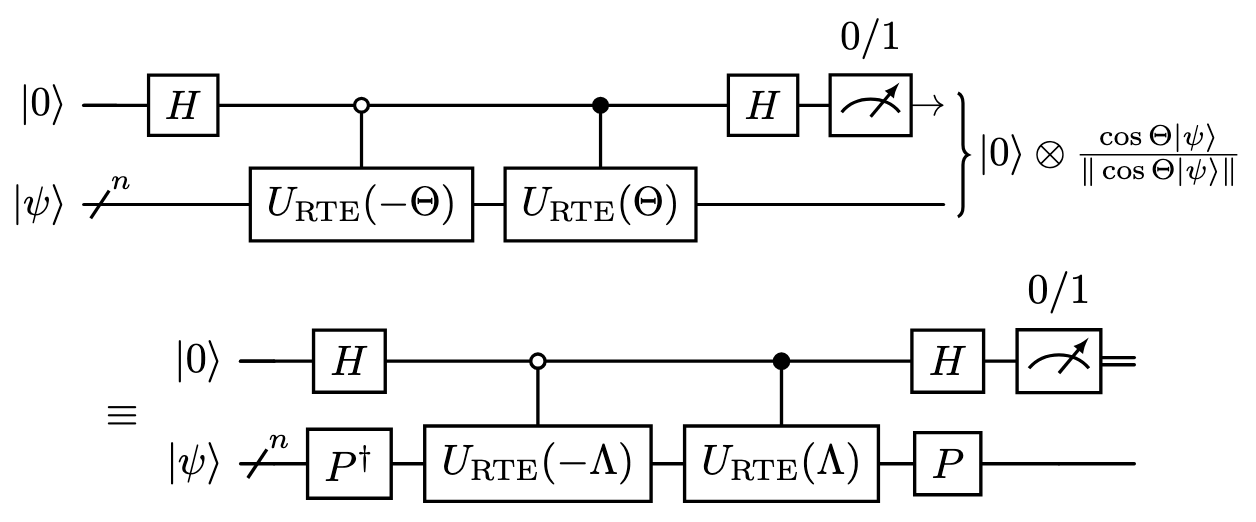
Figure 1: Quantum circuits for PITE based on the cosine function. Here, $U_{\text{RTE}}(\Theta)$ denotes the RTE operator for the operator $\Theta=m_{0}e^{-\Delta\tau\mathcal{H}}$ defined by $U_{\text{RTE}}(\Theta):=e^{-\mathrm{i}\Theta}$. Measuring the ancillary qubit, the PITE operator is implemented with the success probability $m_{0}^{2}\|e^{-\Delta\tau\mathcal{H}}\left|\psi\right\rangle\|^{2}$. The upper circuit is equivalent to the lower one provided that $\Theta$ is diagonalized by $P^{\dagger}\Theta P=\Lambda$.

Although most previous works [28, 29, 30] consider the unitary operation:

$$\widetilde{\mathcal{M}}(\Theta):=\begin{pmatrix}\cos\Theta&-\sin\Theta\\ \sin\Theta&\cos\Theta\end{pmatrix},$$

instead of $\mathcal{M}(\Theta)$, these two implementations of $e^{-\Delta\tau\mathcal{H}}$ based on $\mathcal{M}(\Theta)$ and $\widetilde{\mathcal{M}}(\Theta)$ are equivalent under the following unitary operations (i.e., two single-qubit gates):

$$\mathcal{M}(\Theta)=(Q\otimes I^{\otimes n})\widetilde{\mathcal{M}}(\Theta)(Q^{\dagger}\otimes I^{\otimes n}),$$

where

$$Q:=\frac{1}{\sqrt{2}}\begin{pmatrix}1+\mathrm{i}&0\\ 0&-1+\mathrm{i}\end{pmatrix}.$$

Moreover, thanks to our assumption on $\mathcal{H}$, there exist a unitary operator $P$ and a diagonal matrix $\Lambda$ such that

$$\mathcal{M}(\Theta)=(I\otimes P)\mathcal{M}(\Lambda)(I\otimes P^{\dagger}),\quad\widetilde{\mathcal{M}}(\Theta)=(I\otimes P)\widetilde{\mathcal{M}}(\Lambda)(I\otimes P^{\dagger}).$$

Then, the exact implementation of the PITE operator is demonstrated by the lower circuit in Fig. 1, in which the RTE operators for the diagonal unitary matrices $U_{\text{RTE}}(\pm\Lambda)$ can be realized by using $2^{n}$ phase rotation gates and $2^{n}-2$ CNOT gates with depth $2^{n}$ [34]. On the other hand, Mangin-Brinet et al. [30] used the quantum circuit proposed in [35], and gave the detailed circuit for $\widetilde{\mathcal{M}}(\Lambda)$ by $2^{n}$ $y$-axis rotation gates and $2^{n}$ CNOT gates with depth $2^{n+1}$. Although we also need to calculate the unitary $P$ using the eigenvalue decomposition and implement it by the quantum gates, which is not an easy task in general, there are some kinds of $\mathcal{H}$ such that $P$ is known and can be implemented efficiently within depth $O(n)$. For example, $P=I$ if $\mathcal{H}$ itself is diagonal and $P$ is the shifted/centered quantum Fourier transform (QFT) if $\mathcal{H}$ is generated from the kinetic energy in the first-quantized formalism [36, 28], equivalently, $\mathcal{H}$ is the discretized matrix of the Laplacian with periodic boundary condition.

Let $N=2^{n}$, we find that for the exact implementation of $e^{-\Delta\tau\mathcal{H}}$, one needs $O(N)$ operations of single-qubit and two-qubit gates with depth $O(N)$, which is comparable to the classical counterpart that has a polynomial dependence on $N$. In order to achieve the quantum advantage regarding $N$, we consider an approximate PITE operator whose implementation is efficient for the Hamiltonian appeared in differential equations.

2.1 Alternative approximate PITE

Kosugi et al. proposed an approximate PITE circuit in [28] with a restriction that $m_{0}$ does not equal to $1$. By a shift of energy, this approximate PITE circuit and its derivatives are efficient in the problem of ground state preparation [28, 29, 37]. However, such an approximate PITE and its derivatives are not efficient for the target of ITE because they have an exponentially vanishing success probability $O(m_{0}^{2K})$ as the number of the PITE steps $K$ increases. Since the error of the approximation tends to $\infty$ as $m_{0}$ tends to $1$, one has to take $m_{0}$ away from $1$ (e.g., $m_{0}=0.9$). Then, the success probability decreases rapidly as the number of the steps increases. The details on the approximate PITE [28] are reconsidered in Appendix A. Here, we propose a new approximate PITE with $m_{0}=1$, which we call the alternative approximate PITE, to avoid such a crucial problem.

Let $m_{0}=1$. We rewrite $\Theta=\arccos(m_{0}e^{-\Delta\tau\mathcal{H}})=\arccos(e^{-(\sqrt{\Delta\tau\mathcal{H}})^{2}})$. The notation $\sqrt{\Delta\tau\mathcal{H}}$ makes sense since we assume that $\mathcal{H}$ is a positive semi-definite Hermite operator. Denote $g(x):=\arccos(e^{-x^{2}})$, $x\geq 0$. By the Taylor expansion around $x_{0}\geq 0$ up to the first order, we obtain

$$g(x)=g(x_{0})+g^{\prime}(x_{0})(x-x_{0})+O(|x-x_{0}|^{2}).$$

We calculate directly or use L’Hospital’s rule and obtain

$$\lim_{x\to 0}g(x)=0,\quad\lim_{x\to 0+}g^{\prime}(x)=\lim_{x\to 0+}\frac{2x}{\sqrt{e^{2x^{2}}-1}}=\lim_{x\to 0+}\frac{(2x)^{\prime}}{(\sqrt{e^{2x^{2}}-1})^{\prime}}=\lim_{x\to 0+}\frac{\sqrt{e^{2x^{2}}-1}}{xe^{2x^{2}}}=\sqrt{2}.$$

Taking $x_{0}=0$, we obtain the approximation:

$$\Theta=g(\sqrt{\Delta\tau\mathcal{H}})=\sqrt{2}\sqrt{\Delta\tau\mathcal{H}}+O(\Delta\tau)\approx\sqrt{2\Delta\tau\mathcal{H}}.$$

In other words,

$$e^{-\Delta\tau\mathcal{H}}=\cos(g(\sqrt{\Delta\tau\mathcal{H}}))\approx\cos(\sqrt{2\Delta\tau\mathcal{H}}).$$

Then, we obtain the quantum circuit for the alternative approximate PITE in Fig. 2.

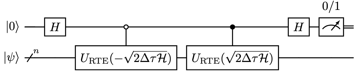
Figure 2: A quantum circuit for the alternative approximate PITE.

We mention the quantum resources used in a single PITE step. The main costs lie in the part of the controlled RTE operator related to $\sqrt{\mathcal{H}}$ for a given Hermite operator $\mathcal{H}$. For such controlled RTE operators, we expect efficient implementations in gate complexity $O(\mathrm{poly}\log N)$, which yields an exponential improvement compared to the exact implementation. In the next section, we will provide the implementation of the RTE of such a half-order operator for the Hamiltonian dynamics in real space. Here, we stick to the justification of the alternative approximate PITE and establish the theoretical error estimate and the success probability.

2.2 Error estimate

For $K\in\mathbb{N}$, we consider the operation of applying the alternative approximate PITE for $K$ times. Assume that $\mathcal{H}$ owes the eigensystem: $\{(\lambda_{k},\psi_{k})\}_{k=0}^{N-1}$ where $0\leq\lambda_{0}\leq\lambda_{1}\leq\cdots\leq\lambda_{N-1}$ are real-valued, and $\{\psi_{k}\}_{k=0}^{N-1}$ forms a complete orthonormal basis of $\mathbb{C}^{N}$. First, we define the error after normalization by

$$\mathrm{Err}:=\left\|\frac{\cos^{K}(\sqrt{2\Delta\tau\mathcal{H}})\left|\psi\right\rangle}{\|\cos^{K}(\sqrt{2\Delta\tau\mathcal{H}})\left|\psi\right\rangle\|}-\frac{e^{-K\Delta\tau\mathcal{H}}\left|\psi\right\rangle}{\|e^{-K\Delta\tau\mathcal{H}}\left|\psi\right\rangle\|}\right\|,$$

where $\left|\psi\right\rangle$ is an initial state. By the triangle inequality, we have

$$\mathrm{Err} \leq\left\|\frac{\cos^{K}(\sqrt{2\Delta\tau\mathcal{H}})\left|\psi\right\rangle}{\|\cos^{K}(\sqrt{2\Delta\tau\mathcal{H}})\left|\psi\right\rangle\|}-\frac{\cos^{K}(\sqrt{2\Delta\tau\mathcal{H}})\left|\psi\right\rangle}{\|e^{-K\Delta\tau\mathcal{H}}\left|\psi\right\rangle\|}\right\|+\frac{\|\cos^{K}(\sqrt{2\Delta\tau\mathcal{H}})\left|\psi\right\rangle-e^{-K\Delta\tau\mathcal{H}}\left|\psi\right\rangle\|}{\|e^{-K\Delta\tau\mathcal{H}}\left|\psi\right\rangle\|}$$

$$\leq\frac{2\|\cos^{K}(\sqrt{2\Delta\tau\mathcal{H}})\left|\psi\right\rangle-e^{-K\Delta\tau\mathcal{H}}\left|\psi\right\rangle\|}{\|e^{-K\Delta\tau\mathcal{H}}\left|\psi\right\rangle\|}.$$

Then, it is sufficient to estimate the error before normalization:

$$\widetilde{\mathrm{Err}}:=\|\cos^{K}(\sqrt{2\Delta\tau\mathcal{H}})\left|\psi\right\rangle-e^{-K\Delta\tau\mathcal{H}}\left|\psi\right\rangle\|.$$

Next, for any $\delta\in[0,1)$, we introduce

$$N_{\delta}(\psi) :=\left\{k\in[\tilde{N}]:=\{0,\ldots,N-1\};\sum_{j=0}^{k-1}|\langle\psi_{j}|\psi\rangle|^{2}<1-\delta,\sum_{j=0}^{k}|\langle\psi_{j}|\psi\rangle|^{2}\geq 1-\delta\right\},$$ (1)

$$\mathcal{K}_{\delta}(\psi) :=\left\{0,\ldots,N_{\delta}(\psi)\right\}\subset[\tilde{N}].$$ (2)

Then, we estimate the upper bound of $\widetilde{\mathrm{Err}}^{2}$ as follows:

$$\quad\widetilde{\mathrm{Err}}^{2}=\sum_{k=0}^{N-1}|\langle\psi_{k}|\psi\rangle|^{2}\left|\cos^{K}(\sqrt{2\Delta\tau\lambda_{k}})-(e^{-\Delta\tau\lambda_{k}})^{K}\right|^{2}$$

$$=\sum_{k=0}^{N-1}|\langle\psi_{k}|\psi\rangle|^{2}\left|(\cos(\sqrt{2\Delta\tau\lambda_{k}}))^{K}-(e^{-\Delta\tau\lambda_{k}})^{K}\right|^{2}$$

$$\leq\sum_{k\in\mathcal{K}_{\delta}}|\langle\psi_{k}|\psi\rangle|^{2}\left|\cos(\sqrt{2\Delta\tau\lambda_{k}})-e^{-\Delta\tau\lambda_{k}}\right|^{2}\left(\sum_{j=0}^{K-1}|\cos(\sqrt{2\Delta\tau\lambda_{k}})|^{j}|e^{-\Delta\tau\lambda_{k}}|^{K-1-j}\right)^{2}+4\delta$$

$$\leq K^{2}\sum_{k\in\mathcal{K}_{\delta}}|\langle\psi_{k}|\psi\rangle|^{2}\left|\cos(\sqrt{2\Delta\tau\lambda_{k}})-e^{-\Delta\tau\lambda_{k}}\right|^{2}+4\delta.$$ (3)

We define

$$h(x):=\cos(x)-e^{-\frac{1}{2}x^{2}},\quad x\in\mathbb{R}.$$

By a direct calculation, we have

$$h^{\prime}(x)=-\sin(x)+xe^{-\frac{1}{2}x^{2}},\quad h^{\prime}(0)=0,$$

$$h^{(2)}(x)=-\cos(x)+(1-x^{2})e^{-\frac{1}{2}x^{2}},\quad h^{(2)}(0)=0,$$

$$h^{(3)}(x)=\sin(x)+(x^{3}-3x)e^{-\frac{1}{2}x^{2}},\quad h^{(3)}(0)=0,$$

$$h^{(4)}(x)=\cos(x)+(-x^{4}+6x^{2}-3)e^{-\frac{1}{2}x^{2}},\quad h^{(4)}(0)=-2,$$

where $h^{(k)}$ denotes the $k$-th derivative of $h$. It is clear that $h\in C^{\infty}(\mathbb{R})$. By employing the Taylor’s theorem near the origin with the Lagrange form of the remainder, we have

$$h(x) =h(0)+h^{\prime}(0)x+\frac{1}{2}h^{(2)}(0)x^{2}+\frac{1}{6}h^{(3)}(0)x^{3}+\frac{1}{24}h^{(4)}(\xi)x^{4}$$

$$=\frac{1}{24}\left(\cos\xi+(-\xi^{4}+6\xi^{2}-3)e^{-\frac{1}{2}\xi^{2}}\right)x^{4},$$

for any $x>0$ and some $\xi\in[0,x]$. For any $k=0,1,\ldots,N-1$, letting $x=\sqrt{2\Delta\tau\lambda_{k}}$, we obtain

$$\left|\cos(\sqrt{2\Delta\tau\lambda_{k}})-e^{-\Delta\tau\lambda_{k}}\right|^{2} =\left|\frac{1}{24}\left(\cos\xi_{k}+(-\xi_{k}^{4}+6\xi_{k}^{2}-3)e^{-\frac{1}{2}\xi_{k}^{2}}\right)(4(\Delta\tau)^{2}\lambda_{k}^{2})\right|^{2}$$

$$=\left|\frac{1}{6}\left(\cos\xi_{k}+(-\xi_{k}^{4}+6\xi_{k}^{2}-3)e^{-\frac{1}{2}\xi_{k}^{2}}\right)\right|^{2}\lambda_{k}^{4}(\Delta\tau)^{4},$$

for some $\xi_{k}\in[0,\sqrt{2\Delta\tau\lambda_{k}}]$. By noting

$$\sup_{x\geq 0}|-x^{2}+6x-3|e^{-\frac{1}{2}x}=3,$$

we obtain

$$\left|\cos(\sqrt{2\Delta\tau\lambda_{k}})-e^{-\Delta\tau\lambda_{k}}\right|^{2} \leq\frac{4}{9}\lambda_{k}^{4}(\Delta\tau)^{4},$$

for any $k=0,1,\ldots,N-1$. We insert this into Eq. (3) and obtain

$$\widetilde{\mathrm{Err}}^{2}\leq\frac{4K^{2}}{9}(\Delta\tau)^{4}\sum_{k\in\mathcal{K}_{\delta}}\lambda_{k}^{4}|\langle\psi_{k}|\psi\rangle|^{2}+4\delta.$$

By setting

$$C_{1}(\left|\psi\right\rangle,\delta):=\left(\sum_{k\in\mathcal{K}_{\delta}}\lambda_{k}^{4}|\langle\psi_{k}|\psi\rangle|^{2}\right)^{1/2},$$

we obtain

$$\widetilde{\mathrm{Err}}\leq\frac{2C_{1}(\left|\psi\right\rangle,\delta)T}{3}\Delta\tau+2\sqrt{\delta},$$ (4)

where $T=K\Delta\tau$. Therefore, we reach the error estimate

$$\mathrm{Err}\leq(4C_{1}(\left|\psi\right\rangle,\delta)T\Delta\tau/3+4\sqrt{\delta})/\|e^{-T\mathcal{H}}\left|\psi\right\rangle\|,$$ (5)

for any $\delta\in[0,1)$.

For a given error bound $\varepsilon>0$, we can choose

$$\delta\leq\left(\frac{\|e^{-T\mathcal{H}}\left|\psi\right\rangle\|\varepsilon}{8}\right)^{2},\quad\text{and}\quad\Delta\tau\leq\frac{3\sqrt{\delta}}{C_{1}(\left|\psi\right\rangle,\delta)T},$$ (6)

so that $\mathrm{Err}\leq\varepsilon$ is fulfilled. If we focus on the order with respect to $\varepsilon$, then we derive $\sqrt{\delta}=O(\varepsilon)$, and thus,

$$\Delta\tau=O\left(\varepsilon C_{1}(\left|\psi\right\rangle,\delta(\varepsilon))^{-1}\right),\quad\text{or equivalently, }\quad K=\Omega\left(\varepsilon^{-1}C_{1}(\left|\psi\right\rangle,\delta(\varepsilon))\right).$$

Since $\lim_{\varepsilon\to 0}\delta(\varepsilon)=0$, we have $C_{1}(\left|\psi\right\rangle,\delta(\varepsilon))=O(\lambda_{N-1}^{2})$ for the worst initial state $\left|\psi\right\rangle$. This means in the worst scenario (i.e., $\delta=0$ and $|\langle\psi_{N-1}|\psi\rangle|^{2}=\Omega(1)$), the total gate complexity is proportional to $K$, and hence, has polynomial dependence on $N$ if $\lambda_{N-1}=\Omega(\mathrm{poly}\,N)$. Here, we introduce a tolerance $\delta>0$, and then we can remove the dependence on $N$ if the overlaps $|\langle\psi_{k}|\psi\rangle|^{2}$ for all large $k$ are sufficiently small (this holds true if the initial state is good enough). Quantitatively, we use $C_{1}(\left|\psi\right\rangle,\delta)$, depending on the tolerance $\delta$ and the initial state $\left|\psi\right\rangle$, to describe the relation between gate complexity and such factors.

2.3 Success probability

We note that the quantum state after applying the alternative PITE for $j$ times is

$$\cos^{j}\left(\sqrt{2\Delta\tau\mathcal{H}}\right)\left|\psi\right\rangle/\left\|\cos^{j}\left(\sqrt{2\Delta\tau\mathcal{H}}\right)\left|\psi\right\rangle\right\|,$$

and the (total) success probability is

$$\mathbb{P}_{1}(\left|0\right\rangle)=\prod_{j=1}^{K}\left\|\cos\left(\sqrt{2\Delta\tau\mathcal{H}}\right)\frac{\cos^{j-1}\left(\sqrt{2\Delta\tau\mathcal{H}}\right)\left|\psi\right\rangle}{\left\|\cos^{j-1}\left(\sqrt{2\Delta\tau\mathcal{H}}\right)\left|\psi\right\rangle\right\|}\right\|^{2}=\|\cos^{K}(\sqrt{2\Delta\tau\mathcal{H}})\left|\psi\right\rangle\|^{2}.$$

By the definition of $\widetilde{\mathrm{Err}}$ and the triangle inequalities, we obtain

$$\|e^{-T\mathcal{H}}\left|\psi\right\rangle\|-\widetilde{\mathrm{Err}}\leq\|\cos^{K}(\sqrt{2\Delta\tau\mathcal{H}})\left|\psi\right\rangle\|\leq\|e^{-T\mathcal{H}}\left|\psi\right\rangle\|+\widetilde{\mathrm{Err}}.$$ (7)

On the other hand, Eqs. (4) and (6) yield

$$\widetilde{\mathrm{Err}}\leq 4\sqrt{\delta}\leq\frac{\varepsilon}{2}\|e^{-T\mathcal{H}}\left|\psi\right\rangle\|.$$

Inserting this into Eq. (7), we estimate the success probability as follows:

$$\left(\frac{2-\varepsilon}{2}\right)^{2}\|e^{-T\mathcal{H}}\left|\psi\right\rangle\|^{2}\leq\mathbb{P}_{1}(\left|0\right\rangle)\leq\left(\frac{2+\varepsilon}{2}\right)^{2}\|e^{-T\mathcal{H}}\left|\psi\right\rangle\|^{2}.$$

By noting that $\|e^{-T\mathcal{H}}\left|\psi\right\rangle\|^{2}$ is independent of the choice of $\Delta\tau$ or $K$, and $(2-\varepsilon)/2$ and $(2+\varepsilon)/2$ are both of order $\Omega(1)$ with respect to $\varepsilon$, we find that the success probability is proportional to $\|e^{-T\mathcal{H}}\left|\psi\right\rangle\|^{2}$, which depends on $\left|\psi\right\rangle$ and $T$, with a proportional constant of almost $1$.

3 Application to advection-diffusion equations

In this section, we investigate the quantum circuit for an ITE operator $e^{-T\mathcal{H}}$ for which $\mathcal{H}$ is a given Hamiltonian matrix corresponding to the following operator appeared in the advection-diffusion equations:

$$\hat{H}=-a\nabla^{2}+\mathbf{v}\cdot\nabla+V,$$ (8)

where $a>0$ is a positive constant, $\mathbf{v}=(v_{1},v_{2},\ldots,v_{d})^{\mathrm{T}}\in\mathbb{R}^{d}$ is a constant vector, and $V=V(\mathbf{x})\in\mathbb{R}$ is a real-valued potential function defined on the cubic domain $[0,L]^{d}$. Here, $d\in\mathbb{N}$ denotes the space dimension and $L>0$ is the length of the domain in each direction. Let $n\in\mathbb{N}$ and $N=2^{n}$. In terms of the grid method, we introduce the grid points, which are described by a $d$-dimensional vector $\mathbf{\ell}=(\ell_{1},\ell_{2},\ldots,\ell_{d})^{\mathrm{T}}\in[\tilde{N}]^{d}:=\{0,1,\ldots,N-1\}^{d}$:

$$\mathbf{p}_{\mathbf{\ell}}=\left(\ell_{1}\frac{L}{N},\ell_{2}\frac{L}{N},\ldots,\ell_{d}\frac{L}{N}\right)^{\mathrm{T}}\in\mathbb{R}^{d}.$$ (9)

Then, the above Hamiltonian can be discretized into an $N\times N$ matrix:

$$H_{N}:=F_{N}\left(D_{N}^{(2)}-\mathrm{i}D_{N}^{(1)}\right)F_{N}^{\dagger}+V_{N},$$ (10)

where

$$F_{N}=\frac{1}{N^{d/2}}\sum_{\mathbf{k}\in[\tilde{N}]^{d}}\sum_{\mathbf{\ell}\in[\tilde{N}]^{d}}\mathrm{exp}\left(\mathrm{i}\frac{2\pi}{N}\left(\mathbf{k}-\frac{N}{2}\right)\cdot\mathbf{\ell}\right)\left|\mathbf{\ell}\right\rangle\left\langle\mathbf{k}\right|,$$

$$D_{N}^{(1j)}=\sum_{\mathbf{k}\in[\tilde{N}]^{d}}v_{j}(2\pi/L)\left(k_{j}-\frac{N}{2}\right)\left|\mathbf{k}\right\rangle\left\langle\mathbf{k}\right|,\quad j=1,\ldots,d,\quad D_{N}^{(1)}=\sum_{j=1}^{d}D_{N}^{(1j)},$$

$$D_{N}^{(2)}=\sum_{\mathbf{k}\in[\tilde{N}]^{d}}a(2\pi/L)^{2}\left|\mathbf{k}-\frac{N}{2}\right|^{2}\left|\mathbf{k}\right\rangle\left\langle\mathbf{k}\right|,$$

$$V_{N}=\sum_{\mathbf{\ell}\in[\tilde{N}]^{d}}V(\mathbf{p}_{\mathbf{\ell}})\left|\mathbf{\ell}\right\rangle\left\langle\mathbf{\ell}\right|=\sum_{\mathbf{\ell}\in[\tilde{N}]^{d}}V\left(\frac{L}{N}\mathbf{\ell}\right)\left|\mathbf{\ell}\right\rangle\left\langle\mathbf{\ell}\right|.$$

For the completeness, we provide the theoretical derivation and its justification of the grid method in Appendix B. We mention that $F_{N}$ and $F_{N}^{\dagger}$ are the shifted QFT of $d$ dimension and its inverse, respectively. According to the definition of $F_{N}$, the $F_{N}$ operation on $dn$ qubits is equivalent to $d$ operations of the one-dimensional shifted QFT on each $n$ qubits.

3.1 Gate complexity

We consider the ITE operator $e^{-TH_{N}}$, where $T>0$ is a given target time. If we directly use the alternative approximate PITE circuit, then we need to know at least a lower bound of the eigenvalues of $H_{N}$, and give an implementation of the RTE operator $U_{\text{RTE}}(\sqrt{2\Delta\tau H_{N}})$, which is not easy since the operator $H_{N}$ is not diagonal. Here, we choose $K\in\mathbb{N}$ and $\Delta\tau=T/K$, and we apply the first-order Suzuki-Trotter formula, for simplicity, to obtain

$$e^{-TH_{N}}=\left(e^{-\Delta\tau H_{N}}\right)^{K} \approx\left(e^{-\Delta\tau F_{N}(D_{N}^{(2)}-\mathrm{i}D_{N}^{(1)})F_{N}^{\dagger}}e^{-\Delta\tau V_{N}}\right)^{K}$$

$$=\left(e^{-V_{0}\Delta\tau}F_{N}e^{\mathrm{i}\Delta\tau D_{N}^{(1)}}e^{-\Delta\tau D_{N}^{(2)}}F_{N}^{\dagger}e^{-\Delta\tau(V_{N}-V_{0}I)}\right)^{K}$$

$$=e^{-V_{0}T}\left(F_{N}e^{\mathrm{i}\Delta\tau D_{N}^{(1)}}e^{-\Delta\tau D_{N}^{(2)}}F_{N}^{\dagger}e^{-\Delta\tau(V_{N}-V_{0}I)}\right)^{K}.$$

Here, $V_{0}:=\min_{\mathbf{x}\in[0,L]^{d}}V(\mathbf{x})$. Then, we can apply the alternative approximate PITE circuit to $\mathcal{H}=D_{N}^{(2)}$ and $\mathcal{H}=V_{N}-V_{0}I$, respectively. Under this approximation, the RTE operators $U_{\text{RTE}}\left(\sqrt{2\Delta\tau D_{N}^{(2)}}\right)$ and $U_{\text{RTE}}\left(\sqrt{2\Delta\tau(V_{N}-V_{0}I)}\right)$ can be implemented with gate complexity $O(\mathrm{poly}\log N)$ since $D_{N}^{(2)}$ and $V_{N}-V_{0}I$ are both diagonal matrices with underlying functions. Then, the quantum circuit for the alternative approximate PITE can be constructed as Fig. 3 in each time step.

Figure 3: A quantum circuit of one time step for the ITE for Hamiltonian $H_{N}$. Here, two approximate PITE circuits are employed. The first one is for the potential part, and the other are for the kinetic part.

In fact, using the well-known strategies in Hamiltonian simulation, we can approximate the diagonals of both diagonal matrices by piecewise polynomials, whose gate complexity is $O(\mathrm{poly}\,n)$. In the case of $d=1$, the operator $U_{\text{RTE}}\left(\sqrt{2\Delta\tau D_{N}^{(2)}}\right)$ can be further efficiently implemented. Note that the eigenvalues of $\sqrt{2\Delta\tau D_{N}^{(2)}}$ are $\lambda_{k,D_{N}^{(2)}}=\sqrt{2a\Delta\tau}(2\pi/L)|k-N/2|$, $k=0,\ldots,N-1$, which is a piecewise linear function of $k$ with only two sub-intervals. Thus, it can be implemented with gate complexity $O(n)$ by the LIU method proposed in [31]. If the potential function $V$ can be efficiently approximated by piecewise linear or quadratic function, then the total gate complexity of a single PITE step is of order $O(n^{2})$. On the other hand, in the case of $d\geq 2$, we can first derive a squared distance register $\left||\mathbf{k}-N/2|^{2}\right\rangle_{2n-1+\lceil\log_{2}d\rceil}$, and then $U_{\text{RTE}}\left(\sqrt{2\Delta\tau D_{N}^{(2)}}\right)$ is implemented by applying a unitary diagonal matrix corresponding to a square root function to the squared distance register. Using piecewise $p$-th degree polynomial approximation for the square root function, the gate complexity is $O(n^{p})$ [31]. If the potential function $V$ are sufficiently smooth and can be efficiently approximated, e.g., localized potential $V=V(|\mathbf{x}-\mathbf{x_{0}}|)$ for some point $\mathbf{x_{0}}\in\mathbb{R}^{d}$, then we can again introduce a squared distance register and implement $U_{\text{RTE}}\left(\sqrt{2\Delta\tau(V_{N}-V_{0}I)}\right)$ with gate complexity $O(\mathrm{poly}\,n)$.

3.2 Error estimate and success probability

We continue to estimate the error between the alternative approximate PITE operator and the exact ITE operator. Define the non-unitary operator of the alternative approximate PITE circuit:

$$U_{\text{AAPITE}}(\Delta\tau)\left|\psi\right\rangle:=\frac{F_{N}e^{\mathrm{i}\Delta\tau D_{N}^{(1)}}\cos\left(\sqrt{2\Delta\tau D_{N}^{(2)}}\right)F_{N}^{\dagger}\cos\left(\sqrt{2\Delta\tau\tilde{V}_{N}}\right)\left|\psi\right\rangle}{\left\|F_{N}e^{\mathrm{i}\Delta\tau D_{N}^{(1)}}\cos\left(\sqrt{2\Delta\tau D_{N}^{(2)}}\right)F_{N}^{\dagger}\cos\left(\sqrt{2\Delta\tau\tilde{V}_{N}}\right)\left|\psi\right\rangle\right\|},$$

for any quantum state $\left|\psi\right\rangle$. Here and henceforth, we denote the shifted $H_{N}$ and $V_{N}$ by $\tilde{H}_{N}=H_{N}-V_{0}I$ and $\tilde{V}_{N}=V_{N}-V_{0}I$ so that the real parts of the eigenvalues of $\tilde{H}_{N}$ and $\tilde{V}_{N}$ are both non-negative. A direct calculation yields

$$U_{\text{AAPITE}}^{K}(\Delta\tau)\left|\psi\right\rangle=\frac{\left(F_{N}e^{\mathrm{i}\Delta\tau D_{N}^{(1)}}\cos\left(\sqrt{2\Delta\tau D_{N}^{(2)}}\right)F_{N}^{\dagger}\cos\left(\sqrt{2\Delta\tau\tilde{V}_{N}}\right)\right)^{K}\left|\psi\right\rangle}{\left\|\left(F_{N}e^{\mathrm{i}\Delta\tau D_{N}^{(1)}}\cos\left(\sqrt{2\Delta\tau D_{N}^{(2)}}\right)F_{N}^{\dagger}\cos\left(\sqrt{2\Delta\tau\tilde{V}_{N}}\right)\right)^{K}\left|\psi\right\rangle\right\|}.$$

For a given initial state $\left|\psi_{(0)}\right\rangle$, we aim at an upper bound of the total error defined by

$$\quad E_{\text{tot}}(\Delta\tau;\left|\psi_{(0)}\right\rangle,K)$$

$$:=\left\|\frac{e^{-K\Delta\tau H_{N}}\left|\psi_{(0)}\right\rangle}{\left\|e^{-K\Delta\tau H_{N}}\left|\psi_{(0)}\right\rangle\right\|}-U_{\text{AAPITE}}^{K}(\Delta\tau)\left|\psi_{(0)}\right\rangle\right\|$$

$$\,=\left\|\frac{e^{-K\Delta\tau(H_{N}-V_{0}I)}\left|\psi_{(0)}\right\rangle}{\left\|e^{-K\Delta\tau(H_{N}-V_{0}I)}\left|\psi_{(0)}\right\rangle\right\|}-\frac{\left(F_{N}e^{\mathrm{i}\Delta\tau D_{N}^{(1)}}\cos\left(\sqrt{2\Delta\tau D_{N}^{(2)}}\right)F_{N}^{\dagger}\cos\left(\sqrt{2\Delta\tau\tilde{V}_{N}}\right)\right)^{K}\left|\psi_{(0)}\right\rangle}{\left\|\left(F_{N}e^{\mathrm{i}\Delta\tau D_{N}^{(1)}}\cos\left(\sqrt{2\Delta\tau D_{N}^{(2)}}\right)F_{N}^{\dagger}\cos\left(\sqrt{2\Delta\tau\tilde{V}_{N}}\right)\right)^{K}\left|\psi_{(0)}\right\rangle\right\|}\right\|$$

$$\,\leq\frac{2\left\|e^{-K\Delta\tau\tilde{H}_{N}}\left|\psi_{(0)}\right\rangle-\left(F_{N}e^{\mathrm{i}\Delta\tau D_{N}^{(1)}}\cos\left(\sqrt{2\Delta\tau D_{N}^{(2)}}\right)F_{N}^{\dagger}\cos\left(\sqrt{2\Delta\tau\tilde{V}_{N}}\right)\right)^{K}\left|\psi_{(0)}\right\rangle\right\|}{\left\|e^{-K\Delta\tau\tilde{H}_{N}}\left|\psi_{(0)}\right\rangle\right\|}$$

$$=\frac{2e^{-K\Delta\tau V_{0}}}{\left\|e^{-K\Delta\tau H_{N}}\left|\psi_{(0)}\right\rangle\right\|}\left\|e^{-K\Delta\tau\tilde{H}_{N}}\left|\psi_{(0)}\right\rangle-\left(F_{N}e^{\mathrm{i}\Delta\tau D_{N}^{(1)}}\cos\left(\sqrt{2\Delta\tau D_{N}^{(2)}}\right)F_{N}^{\dagger}\cos\left(\sqrt{2\Delta\tau\tilde{V}_{N}}\right)\right)^{K}\left|\psi_{(0)}\right\rangle\right\|,$$

for $K\in\mathbb{N}$. Then, it is sufficient to estimate

$$\tilde{E}_{\text{tot}}(\Delta\tau;\left|\psi_{(0)}\right\rangle,K):=\left\|e^{-K\Delta\tau\tilde{H}_{N}}\left|\psi_{(0)}\right\rangle-\left(F_{N}e^{\mathrm{i}\Delta\tau D_{N}^{(1)}}\cos\left(\sqrt{2\Delta\tau D_{N}^{(2)}}\right)F_{N}^{\dagger}\cos\left(\sqrt{2\Delta\tau\tilde{V}_{N}}\right)\right)^{K}\left|\psi_{(0)}\right\rangle\right\|,$$

for $K\in\mathbb{N}$. By denoting $P=F_{N}e^{\mathrm{i}\Delta\tau D_{N}^{(1)}}\cos\left(\sqrt{2\Delta\tau D_{N}^{(2)}}\right)F_{N}^{\dagger}\cos\left(\sqrt{2\Delta\tau\tilde{V}_{N}}\right)$, we have $\|P\|\leq 1$. Hence, a direct estimate yields

$$\tilde{E}_{\text{tot}}(\Delta\tau;\left|\psi_{(0)}\right\rangle,K) =\left\|\sum_{j=0}^{K-1}P^{K-1-j}\left(P-e^{-\Delta\tau\tilde{H}_{N}}\right)(e^{-\Delta\tau\tilde{H}_{N}})^{j}\left|\psi_{(0)}\right\rangle\right\|$$

$$\leq\sum_{j=0}^{K-1}\left\|\left(P-e^{-\Delta\tau\tilde{H}_{N}}\right)(e^{-\Delta\tau\tilde{H}_{N}})^{j}\left|\psi_{(0)}\right\rangle\right\|$$

$$=\sum_{j=0}^{K-1}\tilde{E}_{\text{tot}}(\Delta\tau;\left|\psi_{(j)}\right\rangle,1).$$

Here and henceforth, we denote $\left|\psi_{(j)}\right\rangle=(e^{-\Delta\tau\tilde{H}_{N}})^{j}\left|\psi_{(0)}\right\rangle$ for simplicity. Moreover, we have

$$\tilde{E}_{\text{tot}}(\Delta\tau;\left|\psi_{(j)}\right\rangle,1) =\left\|\left(P-e^{-\Delta\tau\tilde{H}_{N}}\right)\left|\psi_{(j)}\right\rangle\right\|$$

$$\leq\left\|\left(P-F_{N}e^{\mathrm{i}\Delta\tau D_{N}^{(1)}}e^{-\Delta\tau D_{N}^{(2)}}F_{N}^{\dagger}e^{-\Delta\tau\tilde{V}_{N}}\right)\left|\psi_{(j)}\right\rangle\right\|$$

$$\quad+\left\|\left(e^{-\Delta\tau F_{N}(D_{N}^{(2)}-\mathrm{i}D_{N}^{(1)})F_{N}^{\dagger}}e^{-\Delta\tau\tilde{V}_{N}}-e^{-\Delta\tau\tilde{H}_{N}}\right)\left|\psi_{(j)}\right\rangle\right\|$$

$$=:\tilde{E}_{\text{appr}}\left(\Delta\tau;\left|\psi_{(j)}\right\rangle\right)+\tilde{E}_{\text{trot}}\left(\Delta\tau;\left|\psi_{(j)}\right\rangle\right),$$

for $j=0,\ldots,K-1$. We estimate the Suzuki-Trotter error and the approximation error, respectively.

First, we consider the Suzuki-Trotter error, which can be estimated by the following lemma.

Lemma 1.

Let $(X,\|\cdot\|_{X})$ be a Banach space. Assume that $-A$ is a generator of a strongly continuous semigroup $e^{-tA}$ on $X$, and $B$ is a bounded linear operator on $X$. Moreover, we assume

$$\|e^{-tA}\|\leq 1,\quad\|e^{-tB}\|\leq 1,\quad\|e^{-t(A+B)}\|\leq 1,$$ (11)

for all $t>0$. Then, for any $x\in X$ and $t>0$, we have

$$\left\|\left(e^{-tA}e^{-tB}-e^{-t(A+B)}\right)x\right\|_{X}\leq\left(\|B\|^{2}\|x\|_{X}+\frac{1}{2}\max_{0\leq s\leq t}\|[A,B]e^{-s(A+B)}x\|\right)t^{2}.$$

Proof.

We follow the strategy of [38] in which the error estimate of the Strang splitting (second-order splitting) was obtained. According to the variation-for-constant formula, for any $x\in X$ and $t>0$, we have

$$e^{-t(A+B)}x=e^{-tA}x-\int_{0}^{t}e^{-(t-s)A}Be^{-s(A+B)}x\,ds,$$

On the other hand, by the series expansion of $e^{-tB}$, we find

$$e^{-tA}e^{-tB}x=e^{-tA}x-te^{-tA}Bx+R_{1}x,$$

where $\|R_{1}x\|:=\|e^{-tA}(e^{-tB}-I+tB)x\|\leq\frac{t^{2}}{2}\|B\|^{2}\|x\|_{X}$ by Eq. (11). Then, we estimate

$$e^{-tA}e^{-tB}x-e^{-t(A+B)}x=-te^{-tA}Bx+\int_{0}^{t}e^{-(t-s)A}Be^{-s(A+B)}x\,ds+R_{1}x=:R_{2}x+R_{1}x.$$

We introduce a series of operator $W(s):=e^{-(t-s)A}Be^{-s(A+B)}$, $s\geq 0$, then we have

$$R_{2}x=-tW(0)x+\int_{0}^{t}W(s)x\,ds=t^{2}\int_{0}^{1}(1-\theta)W^{\prime}(\theta t)x\,d\theta.$$

Since $W^{\prime}(s)=e^{-(t-s)A}[A,B]e^{-s(A+B)}-e^{-(t-s)A}B^{2}e^{-s(A+B)}$, by Eq. (11), we have

$$\|W^{\prime}(s)x\|\leq\|[A,B]e^{-s(A+B)}x\|+\|B\|^{2}\|x\|_{X},\quad 0\leq s\leq t.$$

Therefore, we have

$$\|R_{2}x\|\leq\frac{t^{2}}{2}\left(\max_{0\leq s\leq t}\|[A,B]e^{-s(A+B)}x\|+\|B\|^{2}\|x\|_{X}\right).$$

Then, the desired estimate follows immediately from the triangle inequality. ∎

Letting $X=\mathbb{C}^{N}$, $A=F_{N}(D_{N}^{(2)}-\mathrm{i}D_{N}^{(1)})F_{N}^{\dagger}$, and $B=\tilde{V}_{N}$ in Lemma 1, we obtain

$$\tilde{E}_{\text{trot}}\left(\Delta\tau;\left|\psi_{(j)}\right\rangle\right) \leq\left(\|\tilde{V}_{N}\|^{2}\left\|\left|\psi_{(j)}\right\rangle\right\|+\frac{1}{2}\max_{0\leq s\leq\Delta\tau}\|[F_{N}(D_{N}^{(2)}-\mathrm{i}D_{N}^{(1)})F_{N}^{\dagger},\tilde{V}_{N}]e^{-s\tilde{H}_{N}}\left|\psi_{(j)}\right\rangle\|\right)(\Delta\tau)^{2}$$

$$\leq C_{2}(\Delta\tau)^{2}.$$

Here, $C_{2}$ is a positive constant depending on $V,V^{\prime},V^{(2)}$ and the a priori bound of the derivative of the solution to the continuous equation (see e.g. Chapter 5 in [27]).

Next, we consider the approximate error. By the triangle inequality, we obtain

$$\tilde{E}_{\text{appr}}\left(\Delta\tau;\left|\psi_{(j)}\right\rangle\right) \leq\left\|\left(F_{N}e^{\mathrm{i}\Delta\tau D_{N}^{(1)}}\cos\left(\sqrt{2\Delta\tau D_{N}^{(2)}}\right)F_{N}^{\dagger}-F_{N}e^{\mathrm{i}\Delta\tau D_{N}^{(1)}}e^{-\Delta\tau D_{N}^{(2)}}F_{N}^{\dagger}\right)e^{-\Delta\tau\tilde{V}_{N}}\left|\psi_{(j)}\right\rangle\right\|$$

$$\quad+\left\|\left(F_{N}e^{\mathrm{i}\Delta\tau D_{N}^{(1)}}\cos\left(\sqrt{2\Delta\tau D_{N}^{(2)}}\right)F_{N}^{\dagger}\right)\left(\cos\left(\sqrt{2\Delta\tau\tilde{V}_{N}}\right)-e^{-\Delta\tau\tilde{V}_{N}}\right)\left|\psi_{(j)}\right\rangle\right\|.$$

Recall that

$$\quad F_{N}e^{\mathrm{i}\Delta\tau D_{N}^{(1)}}\cos\left(\sqrt{2\Delta\tau D_{N}^{(2)}}\right)F_{N}^{\dagger}-F_{N}e^{\mathrm{i}\Delta\tau D_{N}^{(1)}}e^{-\Delta\tau D_{N}^{(2)}}F_{N}^{\dagger}$$

$$=\left(F_{N}e^{\mathrm{i}\Delta\tau D_{N}^{(1)}}F_{N}^{\dagger}\right)\left(\cos\left(\sqrt{2\Delta\tau F_{N}D_{N}^{(2)}F_{N}^{\dagger}}\right)-e^{-\Delta\tau F_{N}D_{N}^{(2)}F_{N}^{\dagger}}\right).$$

We let $K=1$, $\mathcal{H}=F_{N}D_{N}^{(2)}F_{N}^{\dagger}$ and $\tilde{V}_{N}$, respectively, in Sect. 2.2. Then, we have

$$\left\|\left(F_{N}e^{\mathrm{i}\Delta\tau D_{N}^{(1)}}\cos\left(\sqrt{2\Delta\tau D_{N}^{(2)}}\right)F_{N}^{\dagger}-F_{N}e^{\mathrm{i}\Delta\tau D_{N}^{(1)}}e^{-\Delta\tau D_{N}^{(2)}}F_{N}^{\dagger}\right)e^{-\Delta\tau\tilde{V}_{N}}\left|\psi_{(j)}\right\rangle\right\|\leq C_{3}(\Delta\tau)^{2},$$

$$\left\|\left(F_{N}e^{\mathrm{i}\Delta\tau D_{N}^{(1)}}\cos\left(\sqrt{2\Delta\tau D_{N}^{(2)}}\right)F_{N}^{\dagger}\right)\left(\cos\left(\sqrt{2\Delta\tau\tilde{V}_{N}}\right)-e^{-\Delta\tau\tilde{V}_{N}}\right)\left|\psi_{(j)}\right\rangle\right\|\leq C_{4}(\Delta\tau)^{2}.$$

Here, $C_{3}$ depends on the state $e^{-\Delta\tau\tilde{V}_{N}}\left|\psi_{(j)}\right\rangle$ and may depend on the maximal eigenvalue of $D_{N}^{(2)}$ in the worst case scenario. On the other hand, $C_{4}$ depends only on the variation of $V$: $V_{1}-V_{0}$, where $V_{1}:=\max_{\mathbf{x}\in[0,L]^{d}}V(\mathbf{x})\geq V_{0}$. To sum up, we find that

$$\tilde{E}_{\text{tot}}(\Delta\tau;\left|\psi_{(0)}\right\rangle,K)\leq C_{5}K(\Delta\tau)^{2},$$

for a constant $C_{5}$. By noting that $T=K\Delta\tau$, we have

$$E_{\text{tot}}(\Delta\tau;\left|\psi_{(0)}\right\rangle,T/\Delta\tau)\leq\frac{2C_{5}Te^{-TV_{0}}}{\left\|e^{-TH_{N}}\left|\psi_{(0)}\right\rangle\right\|}\Delta\tau=O(\Delta\tau).$$

If we set the error upper bound of $E_{\text{tot}}(\Delta\tau;\left|\psi_{(0)}\right\rangle,T/\Delta\tau)$ by $\varepsilon$, then we have the order of $\Delta\tau=O(\varepsilon)$, and hence $K=\Omega(\varepsilon^{-1})$.

Finally, we consider the total success probability. According to our construction of the alternative approximate PITE circuit, the success probability is given by

$$\mathbb{P}_{\text{tot}}(\left|0\right\rangle)=\left\|\left(F_{N}e^{\mathrm{i}\Delta\tau D_{N}^{(1)}}\cos\left(\sqrt{2\Delta\tau D_{N}^{(2)}}\right)F_{N}^{\dagger}\cos\left(\sqrt{2\Delta\tau\tilde{V}_{N}}\right)\right)^{K}\left|\psi_{(0)}\right\rangle\right\|^{2}.$$

Thanks to the above error estimate, we have

$$\left\|e^{-T\tilde{H}_{N}}\left|\psi_{(0)}\right\rangle\right\|-\tilde{E}_{\text{tot}}(\Delta\tau;\left|\psi_{(0)}\right\rangle,T/\Delta\tau)\leq\sqrt{\mathbb{P}_{\text{tot}}(\left|0\right\rangle)}\leq\left\|e^{-T\tilde{H}_{N}}\left|\psi_{(0)}\right\rangle\right\|+\tilde{E}_{\text{tot}}(\Delta\tau;\left|\psi_{(0)}\right\rangle,T/\Delta\tau),$$

which implies

$$\mathbb{P}_{\text{tot}}(\left|0\right\rangle)\approx\left\|e^{-T\tilde{H}_{N}}\left|\psi_{(0)}\right\rangle\right\|^{2}=e^{2TV_{0}}\left\|e^{-TH_{N}}\left|\psi_{(0)}\right\rangle\right\|^{2},$$

for any sufficiently small $\Delta\tau$. We mention that $\left\|e^{-TH_{N}}\left|\psi_{(0)}\right\rangle\right\|^{2}$ approximates the square of the $L^{2}$-norm of the solution to the continuous equation $(\partial_{t}+\hat{H})u(t)=0$ with a normalized initial condition as $N\to\infty$. In other words, we have $\left\|e^{-TH_{N}}\left|\psi_{(0)}\right\rangle\right\|^{2}$ approaches $\|u(T)\|^{2}/\|u(0)\|^{2}$, which is uniform regarding $N$, as $N$ tends infinity.

3.3 Quantum resources estimation

We sum up the required quantum resources for the total ITE operator $e^{-T\mathcal{H}}$ using the alternative approximate PITE with the first-order Suzuki-Trotter formula in Table 1.

Table 1: Resources requirement for the total ITE operator using the alternative approximate PITE with the first-order Suzuki-Trotter formula.

	CNOT count (Case 1)	CNOT count (Case 2)	Ancilla count
$d=1$	$O((n+n^{p})\varepsilon^{-1})$	$O((n+n^{p}\varepsilon^{-1/(p+1)})\varepsilon^{-1})$	$2$
$d\geq 2$	$O(dn^{p}\varepsilon^{-1-1/(p+1)})$	$O(dn^{p}\varepsilon^{-1-1/(p+1)})$	$2n+2+\lceil\log_{2}d\rceil$

Here, Case 1 denotes the case that the potential function itself is a piecewise polynomial of degree $p\in\mathbb{N}$, while Case 2 denotes the case that the potential function is a piecewise $C^{(p+1)}([0,L]^{d})$ function, so that it can be well approximated by a piecewise polynomial of degree $p$. Although we list only the CNOT count in Table 1, we mention that the circuit depth is at most of the same order as the CNOT count due to our implementation. Moreover, $\varepsilon$ denotes the error bound, and we need additional gate count of $O(\varepsilon^{-1/(p+1)})$ in Case 2, which comes from the approximate error regarding the potential function. For $d\geq 2$, since we approximate a square root function for the kinetic part, we need the additional gate count even for Case 1. Furthermore, for $d=1$, we only need one ancillary qubit for the PITE and another for the potential function. Whereas, for $d\geq 2$, we need the other $2n+\lceil\log_{2}d\rceil$ qubits for constructing the squared distance register. Finally, if we employ a $p$th-order alternative approximate PITE (higher order alternative approximate PITE operators is discussed around Eqs. (17)–(18) in Sect. 5.1) as well as a $p$th-order Suzuki-Trotter formula [39], then the dependence $\varepsilon^{-1}$ can be reduced to $\varepsilon^{-1/p}$ at the cost of increasing the pre-factor according to $p$.

To clarify the result, we have several comments as follows. First, the error bound in Table 1 describes the $l^{2}$-norm of the difference of the normalized approximate PITE operator and the normalized ITE operator, and hence, this table includes only the quantum resources in the approximate ITE of the Hamiltonian (the resources for the statevector preparation and readout are not included). Some comments on the statevector preparation/readout are provided in Appendix C. Second, if we choose $N=\Omega(\log\varepsilon^{-1})$, or equivalently, $n=\Omega(\log\log\varepsilon^{-1})$ such that the discretization error of the Fourier methods (e.g., Appendix B.2 using Lemma 1 in [40]) is also upper bound by $\varepsilon$, then we can insert this into Table 1 to derive a resource estimations with only one parameter, i.e., the error bound $\varepsilon$. Third, our algorithm has a fractional power dependence on $\varepsilon^{-1}$, which seems worse than the logarithmic dependence in [12, 19]. The reason is that we use the multistep strategy, that is, iterate the quantum circuit for each time step. We can also mimic the strategy in [12] to include a quantum register for the temporal variable and improve the dependence on $\varepsilon$. However, this yields a more complicated time-space discretized Hamiltonian whose gate level implementation is not so clear and uses many ancillary qubits. In this paper, keeping in mind the application for the eFTQC, we minimize the use of ancillary qubits and consider the multistep strategy. Another justification of such a power dependence owes to the the result in [41], in which the authors proved that to obtain an approximation of the original solution instead of the normalized one, repetition of $O(\varepsilon^{-1})$ is needed. So it is reasonable to use a quantum algorithm for the ITE with a fractional power dependence on $\varepsilon^{-1}$.

4 Numerical examples

Considering the Hamiltonian $\hat{H}$ given in Eq. (8), a direct application of the alternative approximate PITE operator is to solve the following advection-diffusion equation:

$$\partial_{t}u(\mathbf{x},t)-a\nabla^{2}u(\mathbf{x},t)+\mathbf{v}\cdot\nabla u(\mathbf{x},t)+V(\mathbf{x})u(\mathbf{x},t)=0,\quad\mathbf{x}\in[0,L]^{d},\,0<t\leq T,$$ (12)

where $d\in\mathbb{N}$, $L$ and $T$ are given positive constants which denote the space dimension, the length of the spatial domain, and the final time, respectively. Moreover, $a\in\mathbb{R}_{>0}$ and $\mathbf{v}\in\mathbb{R}^{d}$ are given diffusion coefficient and advection coefficient, respectively, while $V$ is a given zeroth-order (potential) term describing the self-reaction. In the following context, we consider the periodic boundary condition (as we try to adopt our mathematical framework based on the grid/real-space method) with the initial condition:

$$u(\mathbf{x},0)=u_{0}(\mathbf{x}),\quad\mathbf{x}\in[0,L]^{d},$$ (13)

where $u_{0}$ is a sufficiently smooth function. In this paper, the numerical results are simulated by Qiskit [32], a quantum gate-based emulator. Although we mention some efficient techniques [42, 43] for (approximate) encoding in Appendix C, to avoid discussing the additional error from encoding and readout, we realize the quantum statevector preparation and readout by the Qiskit functions: set_statevector() and get_statevector(), respectively, and the success probability is calculated by the $l^{2}$-norm of partial statevector (without stochastic error).

4.1 1D advection-diffusion equation

First, we consider a simple example in 1D case. Let $d=1$, $L=1$, $T=0.1$, $a=0.5$, $\mathbf{v}=5$, and $V=0$. Moreover, we assume $u_{0}(x)=\sin(\pi x)$, $x\in[0,1]$. Actually, in this case, we can solve Eq. (12) analytically using the Fourier series and obtain

$$u(x,t)=\frac{2}{\pi}+\sum_{k=1}^{\infty}-\frac{4}{\pi(4k^{2}-1)}e^{-2\pi^{2}k^{2}t}\cos(2\pi k(x-5t)),\quad x\in[0,1],\ t\in[0,0.1].$$ (14)

As a reference solution, we introduce the truncated solution with a even number $N$:

$$u_{N}(x,t):= \frac{2}{\pi}+\sum_{k=1}^{N/2-1}-\frac{4}{\pi(4k^{2}-1)}e^{-2\pi^{2}k^{2}t}\cos(2\pi k(x-5t))$$

$$-\frac{2}{\pi(N^{2}-1)}e^{-\pi^{2}N^{2}t/2}e^{-\mathrm{i}N\pi(x-5t)},\quad x\in[0,1],\ t\in[0,0.1],$$

which is the solution to Eq. (12) with a truncated initial condition:

$$u_{0,N}(x):=\sum_{k=-N/2}^{N/2-1}\int_{0}^{1}u_{0}(\xi)e^{-\mathrm{i}2\pi k\xi}d\xi\,e^{\mathrm{i}2\pi kx}=\sum_{k=-N/2}^{N/2-1}-\frac{2}{\pi(4k^{2}-1)}e^{\mathrm{i}2\pi kx},\quad x\in[0,1].$$

Here, we define the truncated solution as the linear combination of $N$ dominant Fourier bases ($k=-N/2,-N/2+1,\ldots,N/2-1$), which is the solution using the exact ITE operator if $N=2^{n}$ with some $n\in\mathbb{N}$. Although such truncated solution may be unphysical due to its complex values coming from the third term for any $t>0$, no problem will occur in our mathematical discussion below and it converges to the analytical solution exponentially fast as $N\to\infty$. Furthermore, we call $u_{N}(t):=(u_{N}(p_{0},t),\ldots,u_{N}(p_{N-1},t))^{\mathrm{T}}\in\mathbb{C}^{N}$ the $N$-truncated solution for any $t\in[0,T]$ where $p_{\ell}$, $\ell=0,\ldots,N-1$ are the grid points defined by Eq. (9). Let $\tilde{u}_{N}(t)\in\mathbb{C}^{N}$ be the “$N$-quantum solution” to Eq. (12) using the alternative approximate PITE operator. See Appendix C for the derivation of an “$N$-quantum solution”.

Visualization of the quantum solution We plot the proposed $N$-quantum solution and the $N_{\text{trun}}$-truncated solution at simulation time $t=0.01,0.05,0.1$ in Fig. 4. Here, we take $N_{\text{trun}}=2000$ so that it is almost an analytical solution, and the classical numerical solutions by the FDM in space and the Euler methods in time are also provided for the comparison of the results.

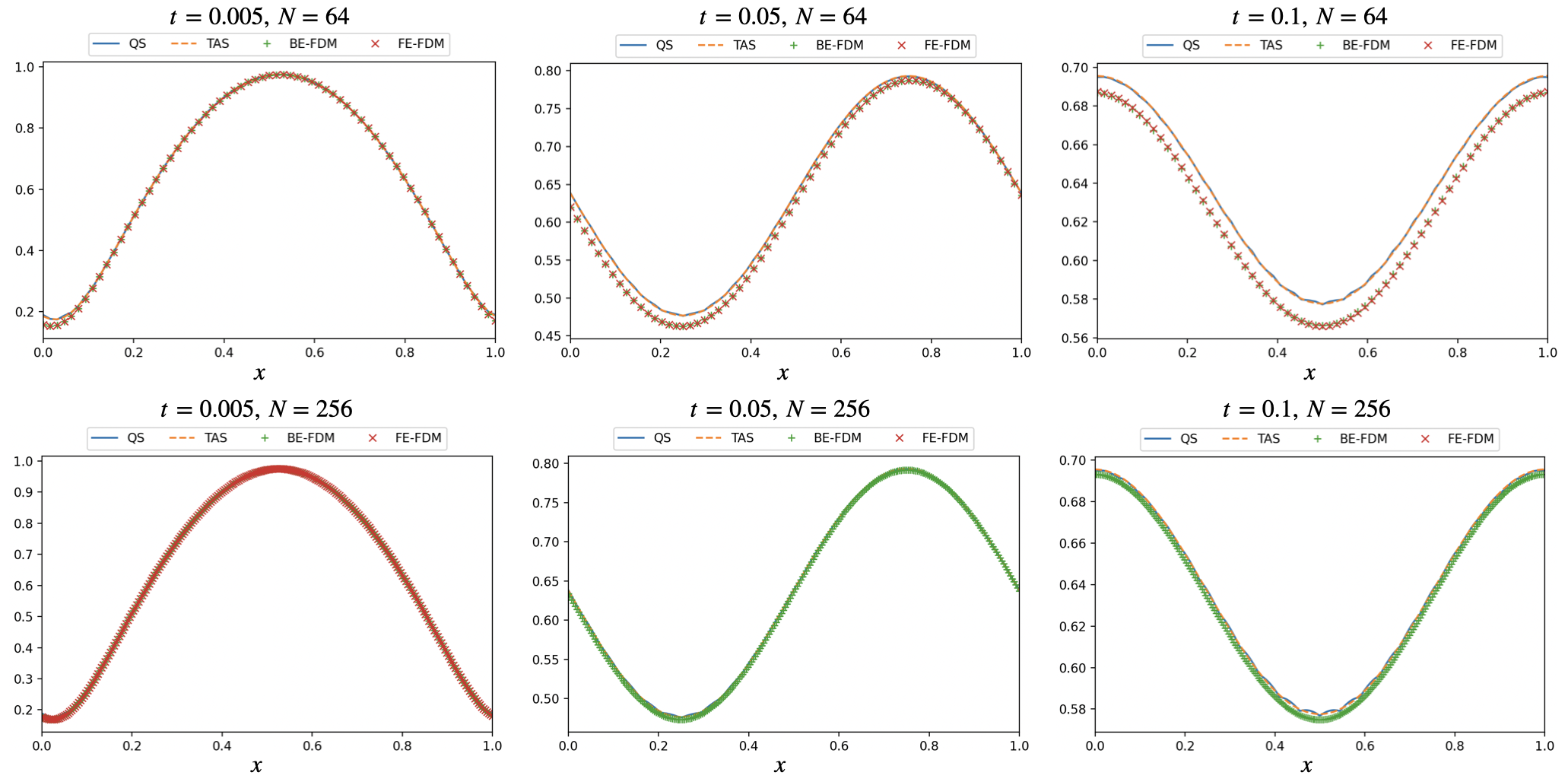
Figure 4: Plot of solutions at time $t=0.005,0.05,0.1$. The $N$-quantum solution (QS), the $N_{\text{trun}}$-truncated analytical solution (TAS), the classical solutions by the backward Euler FDM (BE-FDM) and the forward Euler FDM (FE-FDM) are illustrated by line, dashed line, plus marker, and cross marker, respectively. In the first row, we take $N=2^{6}=64$ while we take $N=2^{8}=256$ in the second row. Moreover, we choose

the time step $\Delta\tau=0.0005$ for the quantum solution, and the time step $\Delta\tau=t/10^{3}$ for the classical FDM solutions.

We find that the proposed quantum solution approaches the analytical solution much better than the classical FDM solutions when the grid parameter $N$ is fixed, especially for a large simulation time and a small grid parameter. The underlying reason is that our quantum solution is based on the FSM whose $N$ describes the number of bases, and thus, it has a better precision than the FDM methods with the same grid parameter $N$. Besides, the quantum solutions in Fig. 4 exhibit arc-like shapes, which owes to the error in the high frequency wave (Fourier coefficients with large indices), and can be relieved by taking smaller $\Delta\tau$. Here, we plot the classical FDM solutions to indicate the best possible performance of the quantum algorithms based on the backward Euler FDM, e.g. [12, 23, 33]. It is clear from Fig. 4 that our quantum solution outperforms the quantum solutions based on the FDMs. More insight discussions and comments on the error are provided in Sect. 4.3, and we compare our proposed quantum algorithm with some other quantum algorithms in Sect. 5.

Linear dependence on time step Next, we plot the $l^{2}$-error between the “$N$-quantum solution” and the $N$-truncated solution in Fig. 5 where we choose $N=2^{6}=64$.

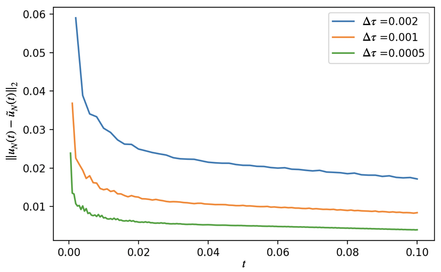
Figure 5: The $l^{2}$-error between the $N$-quantum solution using the alternative approximate PITE operator and the $N$-truncated solution as a time-varying function. Here, $N=2^{6}=64$ and three different time steps of $\Delta\tau=0.002,0.001,0.0005$ are considered in the implementations of the alternative approximate PITE operator. The success probabilities of the approximate PITE circuit are $0.81387$, $0.81395$, and $0.81400$, respectively. The quantum solutions and the success probabilities are both derived by Qiskit emulator [32].

This indicates the convergence of the quantum solution to the truncated solution as the time step $\Delta\tau$ tends to $0$. In this example, we do not have the Suzuki-Trotter error because $V=0$, and we have only the approximation error whose overhead is estimated by $O(\Delta\tau)$ in the previous section. This theoretical linear order can be confirmed numerically, and we put the details into Sect. 4.3.3.

Numerical dependence on diffusion/advection coefficient Finally, we consider the numerical dependence on the diffusion and advection coefficients $a$ and $\mathbf{v}$. The $l^{2}$-errors between the $N$-quantum solutions and the $N$-truncated solutions are shown in Fig. 6.

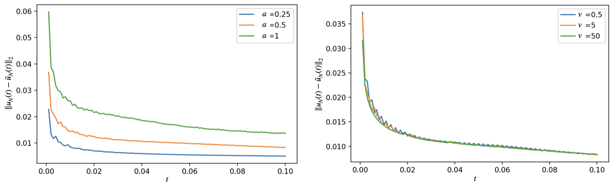
Figure 6: The $l^{2}$-error between the $N$-quantum solution using the alternative approximate PITE operator and the $N$-truncated solution as a time-varying function. Here, $N=2^{6}=64$ and $\Delta\tau=0.001$ are fixed. In the left subplot, three different diffusion coefficients of $a=0.25,0.5,1$ are considered with fixed $\mathbf{v}=5$, while in the right subplot, three different advection coefficients of $\mathbf{v}=0.5,5,50$ are considered with fixed $a=0.5$.

This indicates that the error increases as the diffusion coefficient $a$ becomes larger for small $t$, but it does not depend on the advection coefficient $\mathbf{v}$. The dependence on $a$ can be understood by the following change of variable: $\tilde{t}=at$ to make the diffusion coefficient $1$. Then, keeping $K$ invariant, we have $\widetilde{\Delta\tau}=a\Delta\tau$. This yields an at most linear dependence of $a$ since the error overhead depends linearly on $\widetilde{\Delta\tau}$ (Sect. 3.2). In other words, if we consider the following unified equation by change of variables:

$$\partial_{t}u(\mathbf{x},t)-\nabla^{2}u(\mathbf{x},t)+\mathbf{\bar{v}}\cdot\nabla u(\mathbf{x},t)=0,\quad\mathbf{x}\in[0,L]^{d},\,\bar{t}>0,$$

then the $l^{2}$-error at $\bar{t}=t_{0}$ depends only on $t_{0}$ and $\Delta\tau$, but is independent of $\mathbf{\bar{v}}$.

4.2 2D advection-diffusion equation

Next, we consider a more involved example where we put an absorption potential at the center of the domain. More precisely, we let $d=2$, $L=2\pi$, $T=0.1$, $a=0.5$, $\mathbf{v}=(20,0)^{\mathrm{T}}$, and

$$V(x_{1},x_{2})=\left\{\begin{aligned} &10,&&|x_{1}-\pi|\leq\pi/2\text{ and }|x_{2}-\pi|\leq\pi/2,\\ &0,&&\text{ otherwise. }\end{aligned}\right.$$

Moreover, we consider the initial condition of the Gaussian function:

$$u_{0}(\mathbf{x})=A\,\mathrm{exp}\left(-\frac{|\mathbf{x}-\mathbf{x}_{0}|^{2}}{2\sigma^{2}}\right),$$

with $\mathbf{x}_{0}=(\pi/2,\pi/2)^{\mathrm{T}}$, $\sigma=0.5$ and $A=1$.

Visualization of the quantum solution The $(2^{4},2^{7})$-quantum solutions (see Appendix C for the definition) at several fixed time are illustrated by colormap plots in Fig. 7. The initial source moves in $x_{1}$-direction as expected, and the solution at the center part of the domain decreases rapidly owing to the center absorption potential.

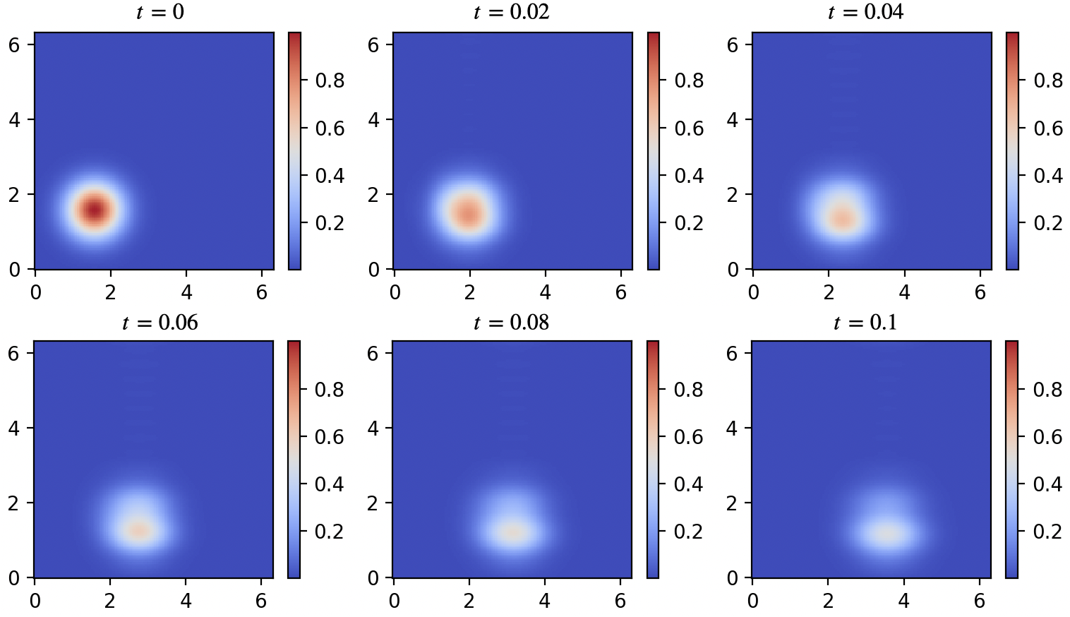
Figure 7: Time evolution of the $(2^{4},2^{7})$-quantum solution using the alternative approximate PITE operator. The quantum solutions at $t=0,0.02,0.04,0.06,0.08,0.1$ are visualized using colormap plots. In each subplot, the $x$ and $y$ axes describe the location in $x_{1}$-direction and $x_{2}$-direction, respectively. The result is simulated by Qiskit, and we take $\Delta\tau=0.0025$ with a second-order Suzuki-Trotter formula.

Dependence on time step With the presence of the spatial varying potential $V$, there is no analytical solution formula. To demonstrate the performance of the alternative approximate PITE, we choose

$$\psi(t):=e^{-tH_{N}}\psi_{\text{init}},\quad\psi(t)\equiv\sum_{\mathbf{\ell}\in[\tilde{N}]^{2}}\psi_{\mathbf{\ell}}(t)\left|\mathbf{\ell}\right\rangle,$$

and

$$u_{N,N_{f}}(t):=\sum_{\mathbf{\tilde{\ell}}\in[\tilde{N}]^{2}}\psi_{\mathbf{\tilde{\ell}}}(t)g_{N}(\mathbf{p}_{\mathbf{\ell}};\mathbf{p}_{\mathbf{\tilde{\ell}}}),\quad\ell\in[\tilde{N}_{f}]^{2},$$

as the reference solution, where $\psi_{\text{init}}$ is the initial state defined by (36), and $g_{N}$ is the two-dimensional pixel function defined in Appendix B.2. According to the discussion in Appendix B, this reference solution converges to the true solution rapidly as $N\to\infty$. Fig. 8 shows the $l^{2}$-error between the $(2^{4},2^{7})$-quantum solution and the reference solution.

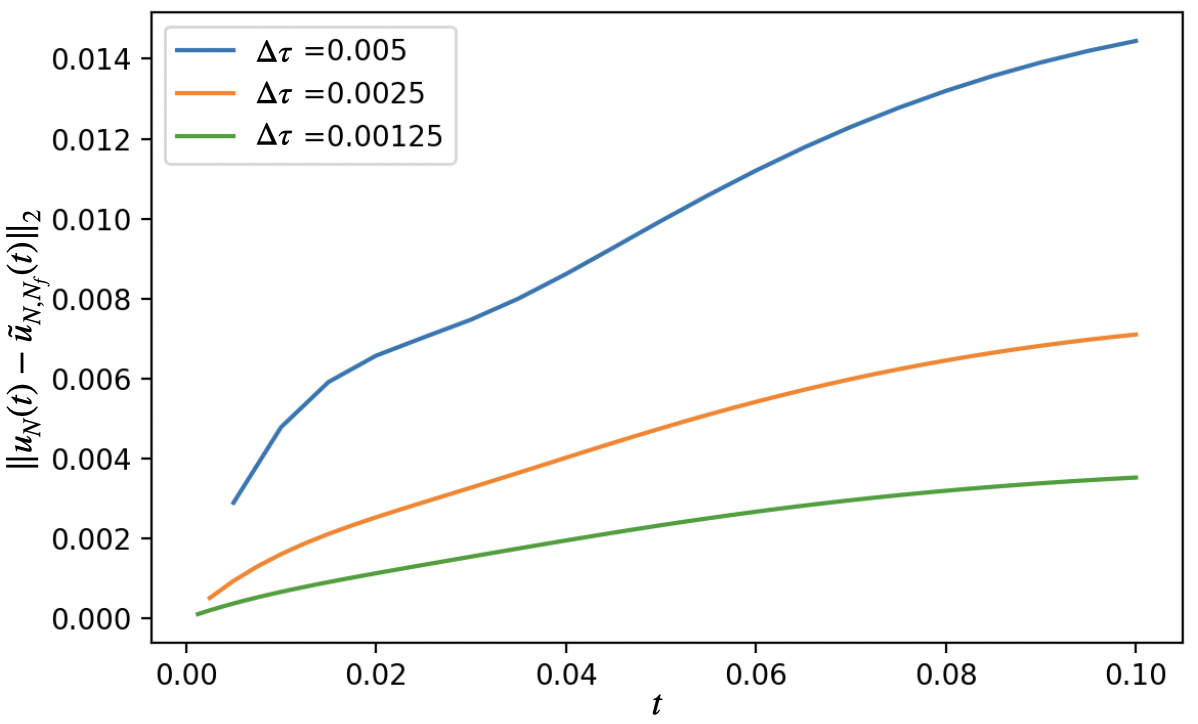
Figure 8: The $l^{2}$-error between the $(2^{4},2^{7})$-quantum solution using the alternative approximate PITE operator and the reference solution as a time-varying function. Here, three different time steps of $\Delta\tau=0.005,0.0025,0.00125$ are considered in the implementations of the alternative approximate PITE operator. The success probabilities of the approximate PITE circuit are $0.26172$, $0.26187$, $0.26194$, respectively. The quantum solutions and the success probabilities are both derived by Qiskit emulator [32], and a second-order Suzuki-Trotter formula is employed in the alternative approximate PITE circuit.

This time, the error comes from both the Suzuki-Trotter formula and the approximation of the PITE operator. In fact, we find that the approximation error depends on the time step linearly, while the Suzuki-Trotter error has a dependence on the time step according to its splitting order. We provide further details on each error regarding the time step in Sect. 4.3.3, 4.3.4. Here, we observe that different from the decreasing errors (with respect to simulation time $t$) in the simple cases of vanishing potential (see Fig. 5), the errors in Fig. 8 increase as $t$ becomes larger. This is consistent with our theoretical overhead in Sect. 3.2 that the error may increase for a long-time simulation when the potential is nonzero.

4.3 Discussion

In this part, we discuss further details on the error of our proposed method using numerical examples. According to the theoretical results in Appendix B.2 and Sect. 3.2, we find the total $l^{2}$-error can be divided into the following three parts:

– Discretization error: This describes the difference between the solution to the original continuous problem and the exact solution to the discretized problem. Here, there is a grid parameter $N$, indicating the size of the matrix, and the error goes to zero as the grid parameter $N$ goes to infinity.

– Suzuki-Trotter error: This error comes from the Suzuki-Trotter formula when the two (or several) operators under considerations are not commutable. Here, there is a time step parameter $\Delta\tau$, and the error goes to zero as the time step $\Delta\tau$ goes to zero.

– Approximation error: This error describes the difference between the numerical solution using the exact PITE circuit and numerical solution using the proposed approximate PITE circuit. Here, there is also a time step parameter $\Delta\tau$, and the error goes to zero as the time step $\Delta\tau$ goes to zero.

In the following context, we investigate the three types of errors regarding the grid parameter $N$ and the time step $\Delta\tau$, respectively.

4.3.1 Discretization error: numerical dependence on grid parameter

We consider the 1D example in Sect. 4.1 and focus on the discretization error. To do this, we take “the analytical solution” (more precisely, we cut off the infinite series in Eq. (14) after $1000$ terms) as the reference solution. In the following plot of error, we compare the quantum solutions using the exact PITE operator to highlight the discretization error under different choices of $N=2^{4},2^{5},2^{6}$.

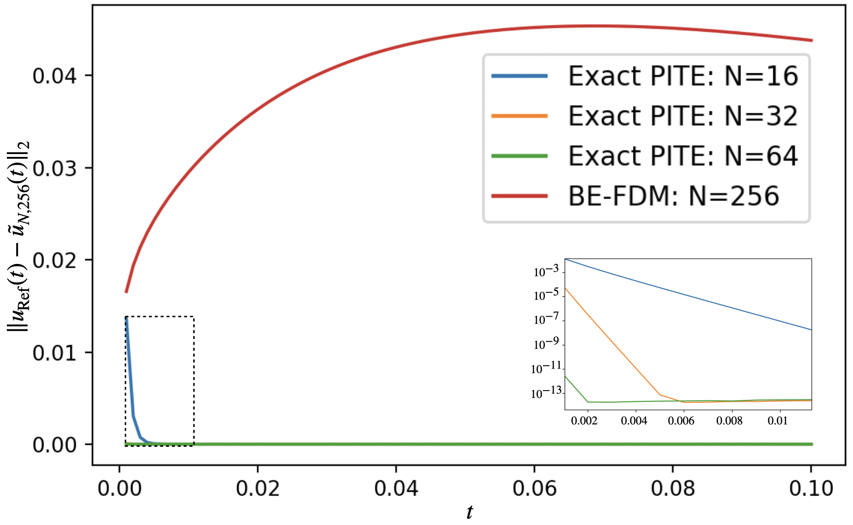
Figure 9: (1D example) Plot of $l^{2}$-error between the quantum solutions and the reference solution. The blue, orange and green lines denotes the $(N,2^{8})$-quantum solutions using the exact PITE with $N=16,32,64$ and $\Delta\tau=10^{-3}$, respectively. The classical solutions by the backward Euler FDM with time step $\Delta\tau=t/10^{3}$ is provided in red.

A zoom-in plot in log-scale is provided to distinguish the orange line and the green line.

According to Fig. 9, we observe that the quantum solutions with small $N=16$ outperform the backward Euler FDM solution with a large $N=256$, which shows that the Fourier spectral approach has better precision than the FDM based approach regarding the grid parameter. Besides, in this example, even $4$ qubits ($N=2^{4}=16$) are enough to derive a sufficiently good solution with error bound $10^{-7}$ after $t\geq 0.01$, and it is clear from the zoom-in plot that the decay of $l^{2}$-error with respect to $N$ is faster than linear, which is actually an exponential decay $O((N/2)^{-N/2})$ according to the theoretical bound in Appendix B.2 using Lemma 1 in [40].

Thanks to the vanishing of the reaction term (i.e., potential $V$), the ITE keeps invariant in any $N$-dimensional spaces $\mathcal{V}_{N}$ spanned by the Fourier bases. In other words, $e^{-t\mathcal{H}}\mathcal{V}_{N}\subset\mathcal{V}_{N}$ for any $t>0$ and $N\in\mathbb{N}$. Since the Fourier coefficients of the initial condition given by a sine function have a rapid decay as the indices increase, only several Fourier coefficients are enough for deriving a good approximation of the initial condition. This is the reason why small $N$ is enough for the example in Sect. 4.1. On the other hand, with the presence of the reaction term in $\mathcal{H}$, $\mathcal{V}_{N}$ is no longer invariant regarding $e^{-t\mathcal{H}}$. This leads to a possible increase of the error as simulation time becomes larger (see e.g., Fig. 8 in Sect. 4.2).

4.3.2 Approximation and/or Suzuki-Trotter errors: numerical dependence on grid parameter

Next, we discuss the $N$ dependence in the approximation and the Suzuki-Trotter errors. Recall Eq. (5) in Sect. 2.2:

$$\text{Err}\leq\left(4C_{1}(\left|\psi\right\rangle,\delta)T\Delta\tau/3+4\sqrt{\delta}\right)/\|e^{-T\mathcal{H}}\left|\psi\right\rangle\|,$$

where

$$C_{1}(\left|\psi\right\rangle,\delta)=\left(\sum_{k\in\mathcal{K}_{\delta}}\lambda_{k}^{4}|\langle\psi_{k}|\psi\rangle|^{2}\right)^{1/2}.$$

By the definition, $C_{1}(\left|\psi\right\rangle,\delta)$ depends also on $N$. As we mentioned, it can increase as $N$ becomes larger, and its upper bound is $\lambda_{N-1}^{2}=O(d^{2}N^{4})$ in the worst scenario. On the other hand, for suitably given initial state $\left|\psi\right\rangle$ and error tolerance $\delta$, the $N$ dependence in the approximation error could be relieved to some extent. In Fig. 10, the approximation error regarding $N$ is demonstrated under the 1D example without potential in Sect. 4.1 and another similar 1D example with a piecewise constant potential function:

$$V(x)=\left\{\begin{aligned} &10,&&|x-1/2|\leq 1/4,\\ &0,&&\text{otherwise},\end{aligned}\right.$$ (15)

where the initial states are both sine functions. Here, we take the reference solution as the one calculated by exact matrix multiplication (i.e., in a similar fashion of the one in Sect. 4.2) to address the errors beyond the discretization error. Our numerical plots imply the $N$-uniform bounds in the case of a good initial state, which means to achieve a given error bound $\delta>0$, we do not need to choose $\Delta\tau\to 0$ as $N\to\infty$. Fig. 10 illustrates that for fixed time step $\Delta\tau$, the $l^{2}$-error seems to converge as $N$ increases. This gives an evidence that the required number of PITE steps $K=t/\Delta\tau$ is uniformly bounded with respect to $N$, and it mainly depends on the initial state and the desired error bound. Since the gate complexity of the approximate PITE circuit is proportional to $K$, Fig. 10 hence implies the exponential speedup regarding the grid parameter $N$ in the quantum solving step, compared to the classical calculations using the matrix multiplications or the optimizations.

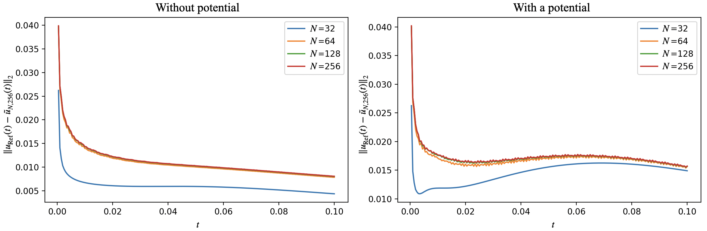
Figure 10: (1D examples) Plot of $l^{2}$-errors between the $(N,2^{8})$-quantum solutions and the reference solution with different $N=32,64,128,256$. Here, we take the same time step $\Delta\tau=0.0005$ in all subplots. The left subplot is for a 1D case without any potential, while the right subplot is for a similar 1D case with an absorption potential in the center part of the domain.

We give a remark on the previous quantum speedup statement. Many existing algorithms for the PDEs, including [13, 41] considered the high precision case and [13] showed the exponential speedup (in the quantum solving step) with respect to the precision $\varepsilon$ by fixing $N=N(\varepsilon)$. However, in many practical applications, the desired error bound is given in advance, or we are interested in the highest precision (largest discretized matrix) under a given computational resource/time. Thus, we have to confirm the quantum speedup regarding the grid parameter $N$. In fact, following the QLSA in [13] using the (best known) Hamiltonian simulation in [44], one can derive an at most polynomial speedup due to the polynomial dependence on $N$ in the conditional numbers for the discretized matrices of many PDEs. Although [10] suggested a preconditioning technique using SPAI preconditioner to reduce the conditional number, there is no guarantee that it works for all discretized matrices [41]. Therefore, a large amount of existing QLSAs do not clarify the exponential speedup in $N$, while [41] showed that exponential speedup is possible only for the quantum solving step provided that the preconditioner works and reduces the conditional number to $O(1)$. In this work, we confirmed the exponential speedup in $N$ for constant coefficient advection-diffusion equation using the approximate PITE based on the grid method (i.e., a specific FSM) for the discretization. Besides, such an exponential speedup in $N$ was confirmed for the constant coefficient hyperbolic equations using an other quantum algorithm in [22].

4.3.3 Approximation error: numerical dependence on time step

According to the theoretical analysis in Sect 3, we find the overhead of the $l^{2}$-error between the quantum solution and the reference solution (truncated solution) is linear in the time step. Here, the reference solution is chosen the exact ITE for the $N$-discretized Hamiltonian $H_{N}$ of the initial state (by the matrix multiplication). In particular, if the potential $V$ vanishes, then the reference solution is the $N$-truncated (analytical) solution which is the projection of the true solution to an $N^{d}$-dimensional subspace $\mathcal{V}_{N}$ spanned by $N^{d}$ eigenvectors of the Laplace operator.

In the numerical example in Sect. 4.1, we plotted the evolution of the $l^{2}$-error for different time steps: $\Delta\tau=0.002,0.001,0.0005$. Here, we provide another plot of the error regarding $\Delta\tau$ at $4$ time points $t=0.002,0.01,0.05,0.1$ in Fig. 11.

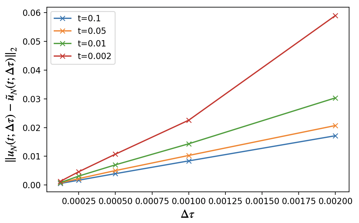
Figure 11: (1D example) Plot of $l^{2}$-errors between the $2^{6}$-quantum solutions and the reference solution regarding time steps $\Delta\tau=0.000125,0.00025,0.0005,0.001,0.002$. The results at $4$ different time points $t=0.002,0.01,0.05,0.1$ are shown in different colors.

We find that for sufficiently large simulation time $t$ ($t=0.05,0.1$) or sufficiently small time step $\Delta\tau$ ($\Delta\tau\leq 0.001$), the linear dependence on the time step is confirmed numerically, which coincides with the theoretical overhead.

Next, we confirm the numerical dependence on time step in the more involved 2D example in Sect. 4.2. Since the potential $V$ does not vanish in this example, we should split the error into the Suzuki-Trotter error and the approximation error. To obtain the approximation error, we introduce an intermediate solution by the quantum circuit in Fig. 3, replacing the approximate PITE circuit by the exact PITE circuit, as the reference solution. The $l^{2}$-errors between the $(2^{4},2^{7})$-quantum solutions and the reference solution are shown in Fig. 12.

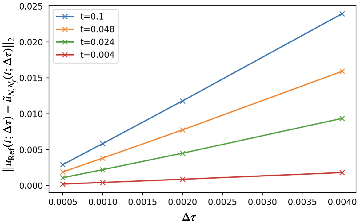
Figure 12: (2D example) Plot of $l^{2}$-errors between the $(2^{4},2^{7})$-quantum solutions and the reference solution regarding time steps $\Delta\tau=0.0005,0.001,0.002,0.004$. The results at $4$ different time points $t=0.004,0.024,0.048,0.1$ are shown in different colors.

A linear dependence on $\Delta\tau$ is again confirmed, but the slope becomes larger for larger simulation time $t$, which is opposite to the 1D example in Fig. 11. According to our comment in the last paragraph of Sect. 4.3.1, this owes to the presence of a function potential $V$. Without providing the details, we also confirmed another 1D example with a quadratic function potential with a peak at the center of the domain, and the result shows that the $l^{2}$-error decreases at first and then keeps increasing. This implies that the approximation error depends on $\Delta\tau$ linearly, but its dependence on $t$ is not clear, which is influenced by the initial condition and the form of the potential.

4.3.4 Suzuki-Trotter error: numerical dependence on time step

Finally, We check the Suzuki-Trotter error numerically, and pay attention to its dependence on the time step. In the 2D example in Sect. 4.2, we choose the reference solution as the exact ITE for the $N$-discretized Hamiltonian $H_{N}$ of the initial condition, which is calculated by the matrix multiplication. Here, we consider the intermediate solution described in Sect. 4.3.3 that has no approximation error as the quantum solution. The intermediate solution is derived by the quantum circuit in Fig. 3, where we substitute the RTE operators

$$U_{\text{RTE}}\left(\pm\sqrt{2\Delta\tau D_{N}^{(2)}}\right)\quad\text{and}\quad U_{\text{RTE}}\left(\pm\sqrt{2\Delta\tau(V_{N}-V_{0}I))}\right)$$

with

$$U_{\text{RTE}}\left(\pm\arccos\left(e^{-\Delta\tau D_{N}^{(2)}}\right)\right)\quad\text{and}\quad U_{\text{RTE}}\left(\pm\arccos\left(e^{-\Delta\tau(V_{N}-V_{0}I))}\right)\right),$$

respectively. Since $D_{N}^{(2)}$ and $V_{N}-V_{0}I$ are both diagonal matrices, for the above RTE operators, we can use the quantum circuit in [34] for the exact implementation. With a first-order Suzuki-Trotter formula:

$$e^{-TH_{N}}\approx e^{-V_{0}T}\left(F_{N}e^{\mathrm{i}\Delta\tau D_{N}^{(1)}}e^{-\Delta\tau D_{N}^{(2)}}F_{N}^{\dagger}e^{-\Delta\tau(V_{N}-V_{0}I)}\right)^{K},$$

or a second-order Suzuki-Trotter formula:

$$e^{-TH_{N}}\approx e^{-V_{0}T}\left(F_{N}e^{\mathrm{i}\Delta\tau D_{N}^{(1)}/2}e^{-\Delta\tau D_{N}^{(2)}/2}F_{N}^{\dagger}e^{-\Delta\tau(V_{N}-V_{0}I)}F_{N}e^{\mathrm{i}\Delta\tau D_{N}^{(1)}/2}e^{-\Delta\tau D_{N}^{(2)}/2}F_{N}^{\dagger}\right)^{K},$$

where $V_{0},D_{N}^{(1)},D_{N}^{(2)}$, and etc. are defined in Sect. 3.1, we plot the $l^{2}$-errors between the quantum solutions and the reference solution regarding $\Delta\tau$ or $\Delta\tau^{2}$ in Fig. 13.

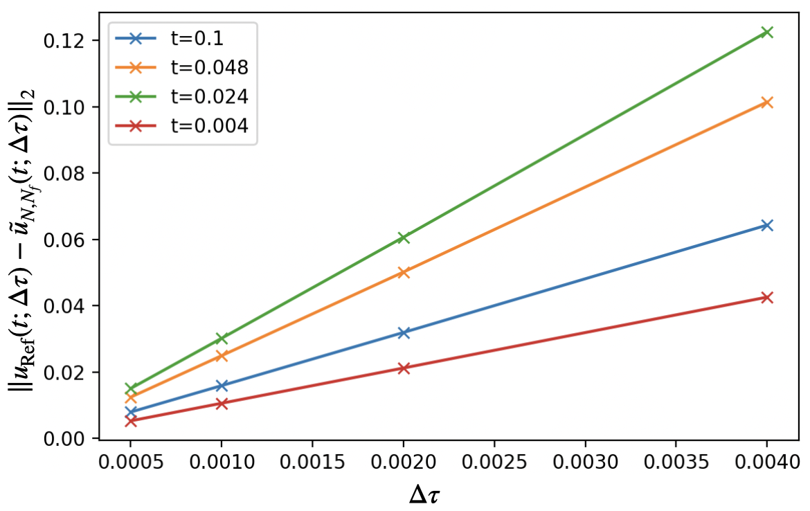
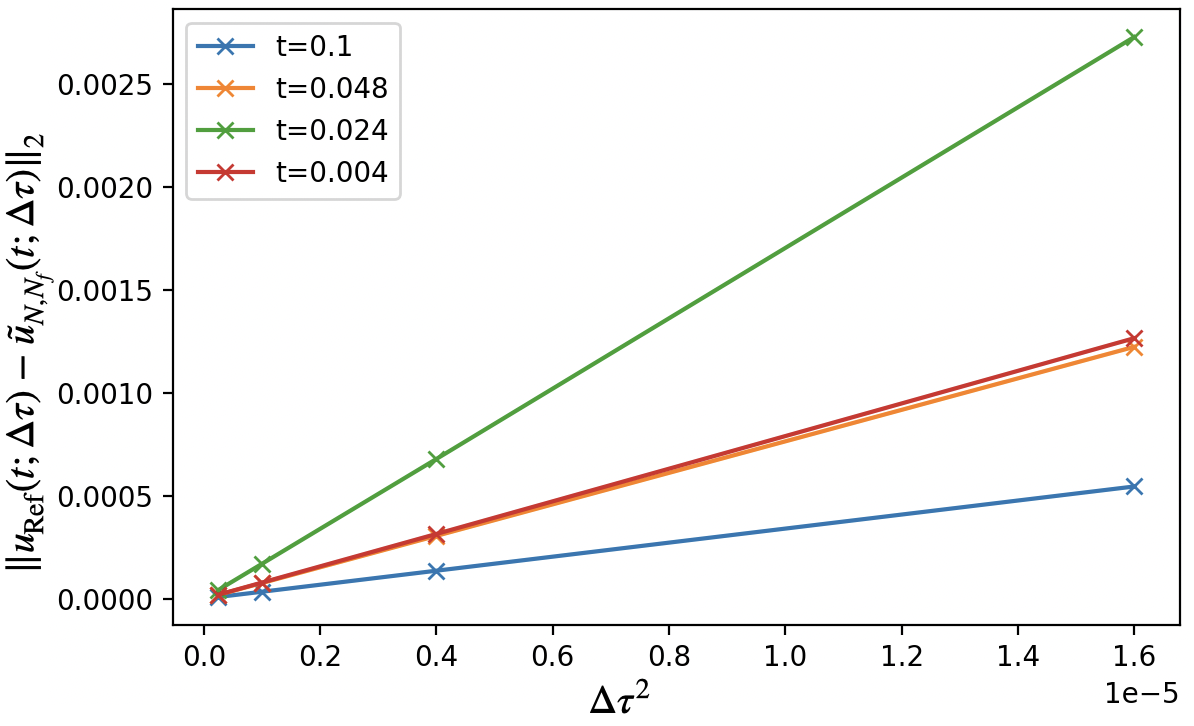
Figure 13: (2D example) Plot of $l^{2}$-errors between the $(2^{4},2^{7})$-quantum solutions without approximate PITE errors and the reference solution regarding time steps $\Delta\tau=0.0005,0.001,0.002,0.004$. In the left subplot, a first-order Suzuki-Trotter formula is employed to derive the quantum solutions, while in the right subplot, a second-order Suzuki-Trotter formula is employed, and the $x$-axis is set to be $\Delta\tau^{2}$. The results at $4$ different time points $t=0.004,0.024,0.048,0.1$ are shown in different colors.

For fixed simulation time $t$, we find linear dependence and quadratic dependence on $\Delta\tau$ for the cases using a first-order Suzuki-Trotter formula and a second-order Suzuki-Trotter formula, respectively. This coincides with the theoretical overheads discussed in Sect. 3.2 and [38], and it seems that the theoretical linear/quadratic dependence on $\Delta\tau$ is not only an overhead but also a sharp estimate. Moreover, we find by focusing on the slopes that the Suzuki-Trotter errors are relatively small for both a small time and a large time. In Fig. 13 for the current 2D example, the Suzuki-Trotter errors are most significant at $t=0.024$, when the initial point source completely enters the zone of absorption (see Fig. 7).

5 Comparisons

In this section, we mainly compare the alternative approximate PITE algorithm with the HHL algorithm and the previous approximate PITE algorithm.

5.1 Theoretical comparison

In this part, we intend to discuss the essential difference between the alternative approximate PITE algorithm and the HHL algorithm. We consider the spatial discretized equation:

$$\partial_{t}\mathbf{v}(t)=-H_{N}\mathbf{v}(t),\quad t>0,$$ (16)

where $H_{N}$ is the discretized matrix in (10). Then, we apply the backward Euler method in time and obtain

$$\frac{\mathbf{\tilde{v}}(m\Delta\tau)-\mathbf{\tilde{v}}((m-1)\Delta\tau)}{\Delta\tau}=-H_{N}\mathbf{\tilde{v}}(m\Delta\tau),\quad m=1,2,\ldots,$$

which implies the updated operation in each time step:

$$\mathbf{\tilde{v}}(m\Delta\tau)=(I+\Delta\tau H_{N})^{-1}\mathbf{\tilde{v}}((m-1)\Delta\tau),\quad m=1,2,\ldots.$$

We regard such a multistep method as the HHL algorithm for the time evolution equations, where one uses an original HHL algorithm to implement the inverse operator in each time step. On the other hand, the alternative approximate PITE solves

$$\mathbf{\hat{v}}(m\Delta\tau)=\cos\left(\sqrt{2\Delta\tau H_{N}}\right)\mathbf{\hat{v}}((m-1)\Delta\tau),\quad m=1,2,\ldots,$$

in each time step, instead. Recalling that the exact solution to Eq. (16) satisfies

$$\mathbf{v}(m\Delta\tau)=e^{-\Delta\tau H_{N}}\mathbf{v}((m-1)\Delta\tau),\quad m=1,2,\ldots.$$

Thus, the theoretical difference between the HHL algorithm and the alternative approximate PITE algorithm lies in the different ways of approximation to the ITE operator in each time step. As a result, to compare their performance with small time step $\Delta\tau$, we only need to check the first several Taylor coefficients of the underlying functions: $g_{\text{exa}}(y)=e^{-y}$ (exact), $g_{\text{HHL}}(y)=1/(1+y)$ (HHL), and $g_{\text{AAP}}(y)=\cos(\sqrt{2y})$ (alternative approximate PITE), respectively. By a direct calculation, we obtain

$$g_{\text{exa}}(y)=1-y+\frac{1}{2}e^{-\xi_{0}}y^{2},\quad\xi_{0}\in[0,y],$$

$$g_{\text{HHL}}(y)=1-y+\frac{1}{(1+\xi_{1})^{3}}y^{2},\quad\xi_{1}\in[0,y],$$

$$g_{\text{AAP}}(y)=1-y+\frac{\sin\sqrt{2\xi_{2}}-\sqrt{2\xi_{2}}\cos\sqrt{2\xi_{2}}}{2(\sqrt{2\xi_{2}})^{3}}y^{2},\quad\xi_{2}\in[0,y].$$

Moreover, we have

$$\lim_{\xi_{0}\to 0}\frac{1}{2}e^{-\xi_{0}}=\frac{1}{2},\ \lim_{\xi_{1}\to 0}\frac{1}{(1+\xi_{1})^{3}}=1,\ \lim_{\xi_{2}\to 0+}\frac{\sin\sqrt{2\xi_{2}}-\sqrt{2\xi_{2}}\cos\sqrt{2\xi_{2}}}{2(\sqrt{2\xi_{2}})^{3}}=\frac{1}{6},$$

which implies that $g_{\text{HHL}}$ and $g_{\text{AAP}}$ are both the first-order approximations of $g_{\text{exa}}$ near the origin $y=0$. Therefore, we conclude that:

(a) The HHL algorithm and the alternative approximate PITE algorithm have comparable precision as the time step $\Delta\tau$ decreases.

(b) The alternative approximate PITE algorithm has slightly better precision for sufficiently small $\Delta\tau$ since the second-order coefficient is closer to the exact one (i.e., $|1/6-1/2|<|1-1/2|$).

(c) One needs a shift of eigenvalues for the alternative approximate PITE algorithm if the smallest eigenvalue of $H_{N}$ is negative, but the HHL algorithm is valid for any Hermitian $H_{N}$ provided that we take a sufficiently small $\Delta\tau$.

We also discuss the gate complexity and the number of ancillary qubits of the two algorithms. If we consider the original HHL algorithm [8] that uses a subroutine of the quantum phase estimation (QPE), then we require the controlled Hamiltonian simulation for $m$ times under the help of an ancillary register of $m$ qubits. Here, $m$ is the number of qubits representing the eigenvalues, which is usually $O(\log N)$. In our setting, the required Hamiltonian simulation for the HHL algorithm is approximated as follows:

$$e^{-\mathrm{i}(I+\Delta\tau H_{N})}\approx e^{-\mathrm{i}\Delta\tau F_{N}(D_{N}^{(2)}-\mathrm{i}D_{N}^{(1)})F_{N}^{\dagger}}e^{-\mathrm{i}(I+\Delta\tau V_{N})}=F_{N}e^{-\mathrm{i}\Delta\tau(D_{N}^{(2)}-\mathrm{i}D_{N}^{(1)})}F_{N}^{\dagger}e^{-\mathrm{i}(I+\Delta\tau V_{N})},$$

which shares the a similar gate complexity as the Hamiltonian simulation for our proposed approximate PITE algorithm. Therefore, using the Suzuki-Trotter formula, we conclude that:

(d) The original HHL algorithm and the proposed approximate PITE algorithm have comparable gate complexity $O(\mathrm{poly}\log N)$, and the alternative approximate PITE is slightly better since its polynomial degree is smaller than that for the HHL algorithm by $1$ (i.e., $2$ uses of controlled Hamiltonian simulation for the alternative approximate PITE, while $m=O(\log N)$ uses of controlled Hamiltonian simulation for the HHL algorithm).

(e) The original HHL algorithm uses $O(\log N)$ ancillary qubits, while our proposed approximate PITE algorithm requires only one ancillary qubit.

Next, we can discuss the original approximate PITE in a similar fashion. The underlying function for the original approximate PITE is

$$g_{\text{OAP}}(y)=\frac{1}{m_{0}}\cos\left(\arccos m_{0}+\frac{m_{0}}{\sqrt{1-m_{0}^{2}}}y\right),\quad m_{0}\in(0,1),$$

which is expanded by

$$g_{\text{OAP}}(y)=1-y-\frac{m_{0}}{2(1-m_{0}^{2})}\cos\left(\arccos m_{0}+\frac{m_{0}}{\sqrt{1-m_{0}^{2}}}\xi\right)y^{2},\quad\xi\in[0,y].$$

Then, we calculate

$$\lim_{\xi\to 0}-\frac{m_{0}}{2(1-m_{0}^{2})}\cos\left(\arccos m_{0}+\frac{m_{0}}{\sqrt{1-m_{0}^{2}}}\xi\right)=-\frac{m_{0}^{2}}{2(1-m_{0}^{2})}\in(-\infty,0),$$

for $m_{0}\in(0,1)$. We find that this is much far away from the desired value $1/2$ than both the alternative approximate PITE and the HHL algorithms, e.g., this limit is $-81/38$ for $m_{0}=0.9$ (the sign itself is opposite). This implies that one needs to take extremely small time step $\Delta\tau$ to make the approximation relatively good. From this point, the alternative approximate PITE is much better than the original one. Besides, according to the theoretical estimate in Appendix A.2, the success probability of the original approximate PITE has a rapid decay since $m_{0}$ is strictly smaller than $1$. This crucial problem is avoided in the alternative approximate PITE. The numerical confirmation can be found in the next subsection.

Furthermore, we can introduce the higher order alternative approximate PITE operators by keeping more terms in the Taylor expansion of $\arccos(e^{-x^{2}})$ near $x=0+$. For example, the second-order alternative PITE operator is given by

$$\cos\left(\sqrt{2\Delta\tau\mathcal{H}}-\sqrt{2\Delta\tau^{3}\mathcal{H}^{3}}/6\right)=e^{-\Delta\tau\mathcal{H}}+O(\Delta\tau^{3}),$$ (17)

and the fourth-order one is

$$\cos\left(\sqrt{2\Delta\tau\mathcal{H}}-\sqrt{2\Delta\tau^{3}\mathcal{H}^{3}}/6+\sqrt{2\Delta\tau^{5}\mathcal{H}^{5}}/120+\sqrt{2\Delta\tau^{7}\mathcal{H}^{7}}/336\right)=e^{-\Delta\tau\mathcal{H}}+O(\Delta\tau^{5}).$$ (18)

The above coefficients come from the Taylor expansion:

$$\arccos(e^{-x^{2}})=\sqrt{2}x-\frac{\sqrt{2}}{6}x^{3}+\frac{\sqrt{2}}{120}x^{5}+\frac{\sqrt{2}}{336}x^{7}+\cdots.$$

We plot the underlying functions of the different approximations of the ITE operator to provide an intuitive comparison of the above mentioned methods. Under a relatively large scale $[0,1]$ and a relatively small scale $[0,0.01]$, Fig. 14 shows that the errors of the different methods do not change a lot if the time step $\Delta\tau$ is sufficiently close to $0$, while the higher order alternative PITE operators give good approximation even for relatively large $\Delta\tau$.

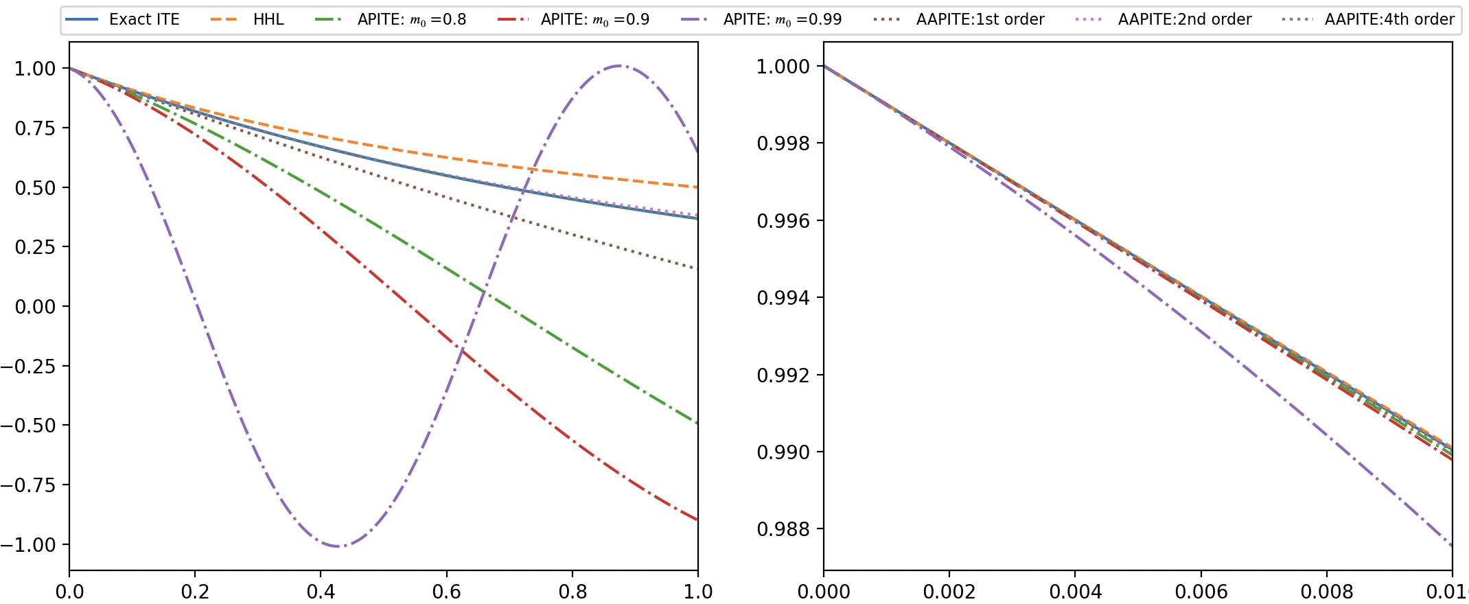
Figure 14: Plot of the underlying functions of different approximations. The $x$-axis is the variable and the $y$-axis denotes the underlying functions of the different approximations. The functions in a relatively large interval $[0,1]$ are plotted in the left subplot, while those near $x=0$ are plotted in the right subplot.

Since the gate complexity of the quantum algorithm is proportional to $\Delta\tau^{-1}$, the higher order alternative approximate PITE operators can be more efficient if its implementation does not require substantially additional gate complexity than the first-order alternative approximate PITE operator. In practice, we conjecture that there is an optimal order, which may depend on the differential equation, the error bound, as well as the order of the Suzuki-Trotter formula.

We end up this section by a remark on some other QLSAs. In [13], the authors proposed a modified algorithm of the HHL algorithm using the LCU techniques in [45, 44] to implement the non-unitary operation $A^{-1}$. One can apply such an idea to our problem by taking $A=I+\Delta\tau H_{N}$. The LCU uses multiple ancillary qubits whose number depends on the desired non-unitary operation and the error bound. Besides, although [13] stated a better dependence regarding the error bound $\varepsilon$: $O(\log\varepsilon^{-1})$ in the gate complexity, this does not count the temporal error from the Euler methods in our problem. By multiplying the number of time steps $T/\Delta\tau=O(\varepsilon^{-1})$, we find that using the algorithm in [13] gives a comparable gate complexity to our proposed one, and it requires more ancillary qubits than ours. On the other hand, there are ideas of applying the truncated Taylor series [45, 12], Dyson series [19] in the time variable and derive a larger time-space discretized Hamiltonian matrix to reach the currently sharp order $O(\log\varepsilon^{-1})$ in the gate complexity, but such methods require more ancillary qubits and more complicated implementation of the discretized Hamiltonian matrix, and they share the problem of small probability to obtain the solution at a specific time. Moreover, there are QLSAs giving other approximate implementations of the ITE operator $e^{-TH_{N}}$, e.g., [15]. However, to the authors’ best knowledge, we do not find any references on the quantum gate level implementations of the ideas in [15] for some detailed partial differential equations. As a result, we are not sure about the comparison between our PITE algorithm and the QLSAs therein regarding the required quantum resources, including the gate count and circuit depth, which needs to be investigated in a proceeding work.

5.2 Numerical comparison by case study

In this part, we compare our proposed approximate PITE algorithm with some previous works in detail using 1D numerical examples.

Comparison with previous work using the HHL algorithm/a VQA We compare our quantum algorithm with a previous work for a one-dimensional advection-diffusion equation [33], where the authors compared two quantum algorithms. One of them is a QLSA based on the HHL algorithm and the other is a VQA. According to Fig. 6 in [33], the simulation results of both the QLSA and the VQA are comparable in the mean squared error (MSE).

Here, we check the MSE of our quantum solution in the setting of [33]. Let $d=1$, $L=1$, $a=1$, $\mathbf{v}=10$, $T=0.04$, and $V=0$. Moreover, the initial condition is set to be the shifted Dirac delta function $\delta(x-L/2)$ which can be rewritten in the following Fourier series:

$$u_{0}(x)=\frac{1}{L}+\sum_{k=1}^{\infty}\frac{2}{L}\cos(k\pi)\cos\left(\frac{2k\pi}{L}x\right),\quad x\in[0,L].$$

Then, the analytical solution is known as follows:

$$u(x,t)=\frac{1}{L}+\sum_{k=1}^{\infty}\frac{2}{L}\cos(k\pi)\cos\left(\frac{2k\pi}{L}(x-vt)\right)\mathrm{exp}\left(-a\left(\frac{2k\pi}{L}\right)^{2}t\right),\quad x\in[0,L],\ t>0,$$

and we define the truncated analytical solution by

$$u_{N_{\text{trun}}}(x,t):=\frac{1}{L}+\sum_{k=1}^{N_{\text{trun}}}\frac{2}{L}\cos(k\pi)\cos\left(\frac{2k\pi}{L}(x-vt)\right)\mathrm{exp}\left(-a\left(\frac{2k\pi}{L}\right)^{2}t\right),\quad x\in[0,L],\ t>0,$$

with a parameter $N_{\text{trun}}\in\mathbb{N}$. We take sufficiently large $N_{\text{trun}}=1000$ above and regard it as the reference solution, which is almost an analytical solution because of the exponentially decay of the high frequency (i.e., large $k$) parts.

First, we plot the proposed quantum solutions with different parameters at two time points $t=0.005$ and $t=0.04$ in Fig. 15.

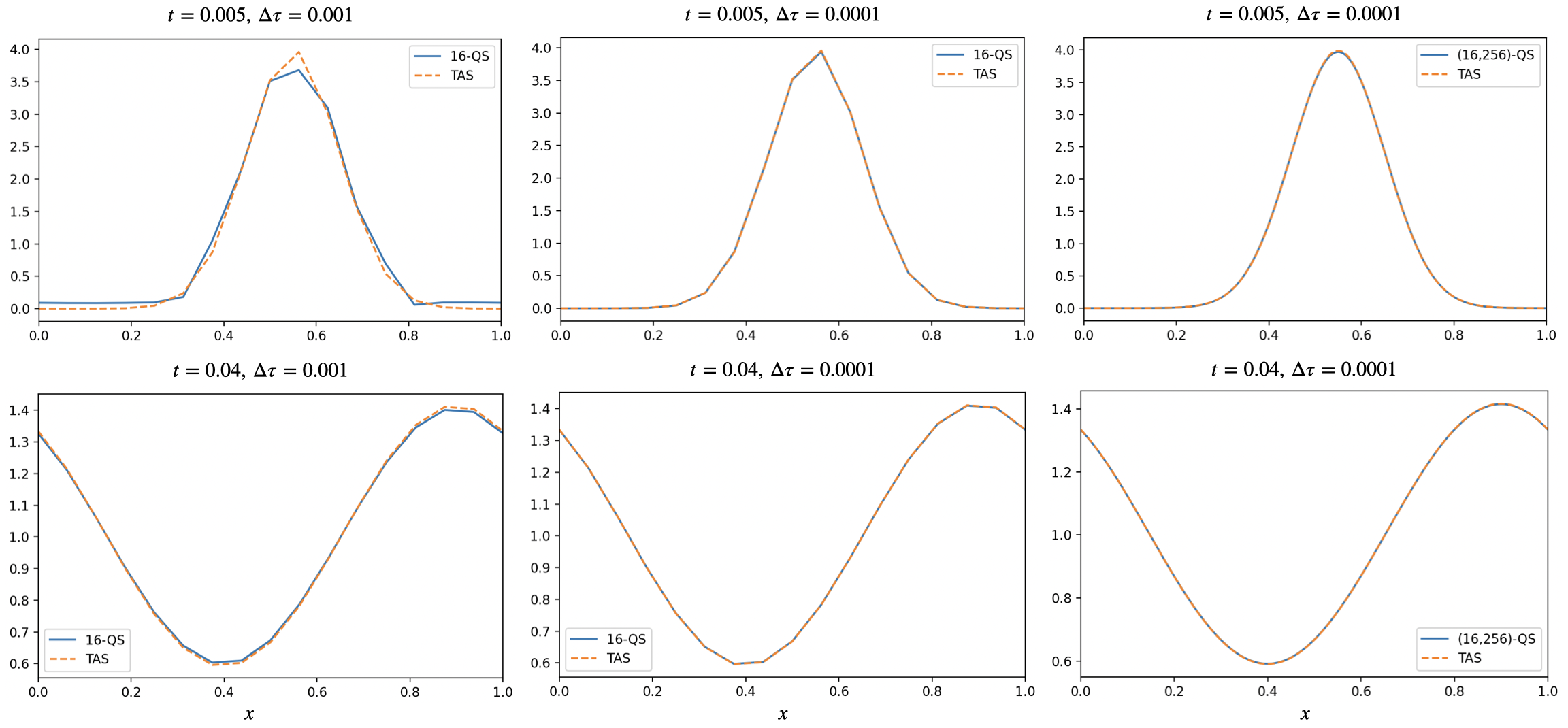
Figure 15: Proposed quantum solutions with different time steps $\Delta\tau=0.001,0.0001$ at $t=0.005,0.04$. The quantum solutions at $t=0.005$ is shown in the first row, while the solutions at $t=0.04$ is shown in the second row. The first column gives the $2^{4}$-quantum solutions with a relatively large time step $\Delta\tau=0.001$, the second column gives the $2^{4}$-quantum solutions with a smaller $\Delta\tau=0.0001$, and the third column gives the $(2^{4},2^{8})$-quantum solutions with $\Delta\tau=0.0001$ for comparison. In each subplot, the reference solution (TAS) is plotted in dashed line.

All the quantum solutions fit the analytical solution well. Focusing on the first two columns, we find that if a smaller time step $\Delta\tau$ is chosen, then the quantum solution approximates the analytical solution even better. The third column in Fig. 15 gives the $(2^{4},2^{8})$-quantum solutions, which indicates that our quantum solution using only $4$ qubits (one ancillary qubit is not counted) provides good approximation to the analytical solution on a $2^{8}$ grid.

Next, we provide a quantitative analysis by plotting the MSEs between the quantum solutions and the reference solution. Again, we choose two different time steps $\Delta\tau=0.001$ and $\Delta\tau=0.0001$. The results are demonstrated in Fig. 16.

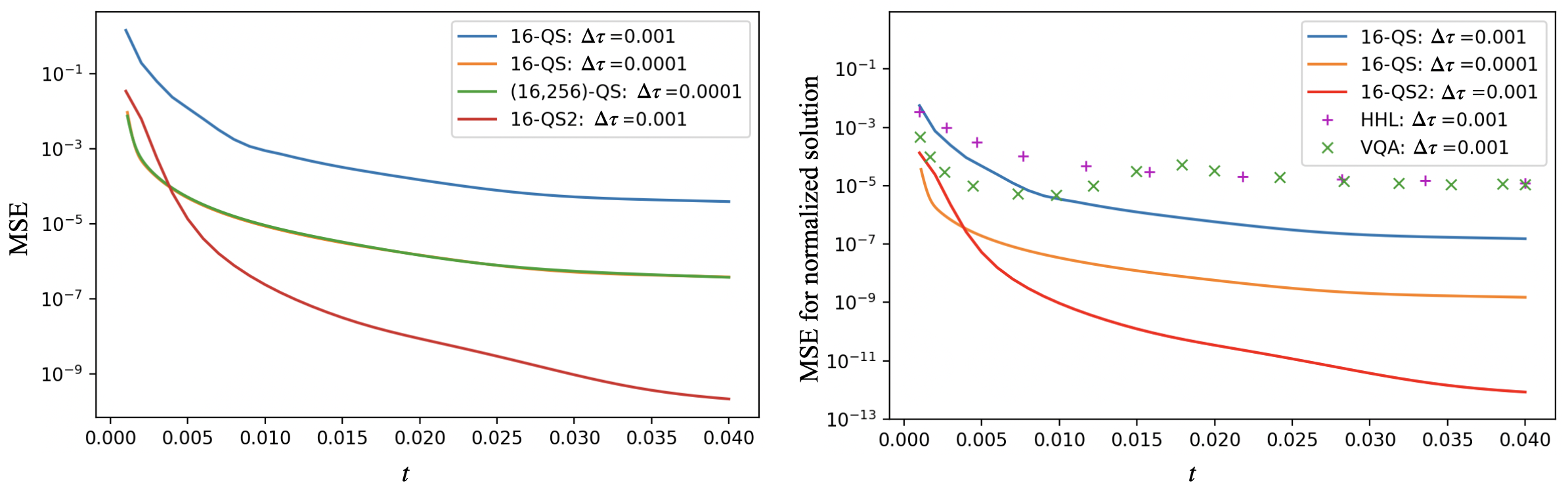
Figure 16: MSEs between the quantum solutions and the reference solution. The results by several quantum solutions are plotted in different colors, while $4+1$ qubits are used to derive the quantum solutions in all cases. Here, $16$-QS2 indicates a second-order alternative approximate PITE, which implements the operation in Eq. (17). The left subplot describes the MSEs between the quantum solutions and the reference solution. The right one describes the MSEs between the normalized quantum solutions and the normalized reference solution using our proposed quantum solution and the HHL algorithm and the VQA in [33]. The data of the HHL algorithm and the VQA are extracted from Fig. 6 in [33] by the application PlotDigitizer [46].

We find that the MSEs are relatively large near the initial time, and they decreases as $t$ becomes larger. Regarding the theoretical estimation of the $l^{2}$-error in Sect. 3.2, the MSE has a quadratic dependence on the time step $\Delta\tau$, which is also observed in Fig. 16 by comparing the blue and orange lines. Note that the orange line almost coincides with the green line in the left subplot of Fig. 16. This implies that the post-processing step in Appendix C.3 enables us to obtain the solutions in a finer grid keeping almost the same precision (MSE). To compare with the results in [33], we provide also the MSEs between the normalized quantum solutions and the normalized reference solution. Here, we choose the same normalized solutions as those in [33], that is, we divide the quantum/reference(analytical) solution by the grid parameter $N$ so that the $l^{2}$-norm of the initial state is normalized to $1$. By choosing the same $\Delta\tau=0.001$, we have a comparable result to Fig. 6 in [33] (see the blue line in the right subplot in Fig. 16). More precisely, we have similar MSE as the HHL and one-order worse MSE than the VQA near $t=0$, while we obtain two-order better MSE than both algorithms near $t=0.04$. Besides, we can achieve further better precision by choosing small $\Delta\tau$ for fixed $N=16$ (see the orange line), and obtain a precision of $10^{-9}$ at $t=0.04$, which is a huge improvement than the HHL algorithm and the VQA in [33].

Our algorithm outperforms the ones in [33] even for more complicated case of non-vanishing potential (see Fig. 17 where our quantum solution and the backward Euler FDM solution are plotted). The reason is as follows. With reference to the well-known theoretical error estimation of the Euler FDMs, the $l^{2}$-error scales as $O(\Delta\tau)+O(N^{-2})$, which means the MSE is $O(N^{-1}\Delta\tau^{2})+O(N^{-5})$. On the other hand, by the theoretical estimations in Sect. 3.2 for both the approximation error and the Suzuki-Trotter error, as well as the theoretical bound of the discretization error (see Lemma 1 in [40]), the $l^{2}$-error of the proposed alternative approximate PITE is $O(\Delta\tau)+O((N/2)^{-N/2})$. This implies that the MSE is $O(N^{-1}\Delta\tau^{2})+O(N^{-1}(N/2)^{-N})$, whose second part has an exponential decay in $N$. These theoretical estimates explain the superiority (in $N$) of our algorithm over the ones in [33] based on the Euler FDMs. Moreover, we can further consider the second-order alternative approximate PITE operator in Eq. (17). As long as we consider the Hamiltonian dynamics in real space, the quantum circuit for the second-order alternative approximate PITE operator can be similarly implemented as the proposed (first-order) alternative approximate PITE operator because the kinetic part is still diagonal in the Fourier domain and the potential part is diagonal. The only difference is that we need to implement a third-degree polynomial function, which can be precisely realized by the polynomial phase gates described in [37, 31] using $O(\mathrm{poly}\log N)$ quantum gates with depth $O(\mathrm{poly}\log N)$. The MSE for the $16$-quantum solution using the second-order alternative approximate PITE is denoted by the red line in Fig. 16. Owing to the higher-order dependence on $\Delta\tau$, the method based on the second-order approximate PITE greatly outperforms the previous work and achieves a precision of $10^{-12}$ at $t=0.04$. Combining such a high-order approximate PITE operator (see the discussion around Eqs. (17)–(18)) with a high-order Suzuki-Trotter formula, we can derive a quantum solution with $l^{2}$-error of $O(\Delta\tau^{p})+O((N/2)^{-N/2})$ for any $p\geq 2$ at the cost of larger gate count/depth (but still of the order $O(\mathrm{poly}\log N)$).

According to the above discussions, we have shown the better performance using our proposed algorithm than the HHL algorithm and the VQA based on the Euler FDMs in [33] when $N$ is fixed. For the total number of qubits, we use only $1+\log_{2}N$, that is, $\log_{2}N$ qubits for the spatial discretization and another ancillary qubit for the approximate PITE (we do not need more qubits because $d=1$ and $V=0$). This is the same as that for the VQA and smaller than that for the HHL algorithm, that is, $1+n_{q}+\log_{2}N$ where $n_{q}=O(\log_{2}N)$ is the number of ancillary qubits for the QPE. As for the execution time, since our algorithm needs much less classical computations, the total execution time for simulating the above example (by Qiskit with more than $400$ PITE steps) requires less than $3$ minutes on a laptop (MacBook Pro, Z16R0004VJ/A, FY2022, Apple M2, 8 Cores, 16GB), much faster than the VQA (a half hour to several hours, see Table C.1 in [33]). The circuit depth of our algorithm in each time step is $O(\log N)$ (in the case of $d=1$ and $V=0$, the main part of our quantum circuit is a shifted QFT, its inverse, a RTE operator for a linear function based diagonal unitary, and two controlled RTE operators for a piecewise-linear-function-based diagonal unitary), which is smaller than that for the HHL algorithm because even the QPE part of the HHL algorithm requires $O(\log N)$ queries to the controlled RTE operator for the discretized Hamiltonian.

As mentioned in the last subsection, the alternative approximate PITE algorithm theoretically provides a comparable result to the HHL algorithm provided that the same spatial discretization is used. Here, we find that our proposed algorithm using the grid method (i.e., a specific FSM) can achieve further better performance than the HHL algorithm based on the FDMs. Although the FSM is not flexible in boundary conditions compared to the other discretization methods including the FDMs, the finite element methods (FEMs), etc., it is compatible with the first-quantized Hamiltonian simulation so that the corresponding quantum circuit for solving the PDEs can be efficiently and explicitly constructed.

Comparison with the previous approximate PITE We also compare the alternative approximate PITE with the original approximate PITE in [28] and its derivative in [29] (variable-time-step PITE or VS-PITE) that takes varying time steps $\{\Delta\tau_{j}\}_{j=1}^{K}$ using a more involved case of $V\not=0$. Let $d=1$, $L=1$, $T=0.1$, $a=0.5$, $\mathbf{v}=5$, and $u_{0}(x)=\sin(\pi x)$, $x\in[0,1]$. Moreover, we consider the piecewise constant potential function Eq. (15) in Sect. 4.3.2, which has large absorption around the center of the domain. In such a case with non-vanishing potential, there is no analytical formula for the solution in general. We first check the classical solutions by the backward Euler FDM with different grid parameters $N=64,256,1024,4096$ to find that the solutions have small changes after $N\geq 1024$, and hence, we take the one with the largest $N=4096$ as the reference solution. Then, we demonstrate the quantum solutions using the original approximate PITE in [28], the variable-time-step approximate PITE in [29], and the alternative approximate PITE under the grid $N=2^{6}=64$ in Fig. 17.

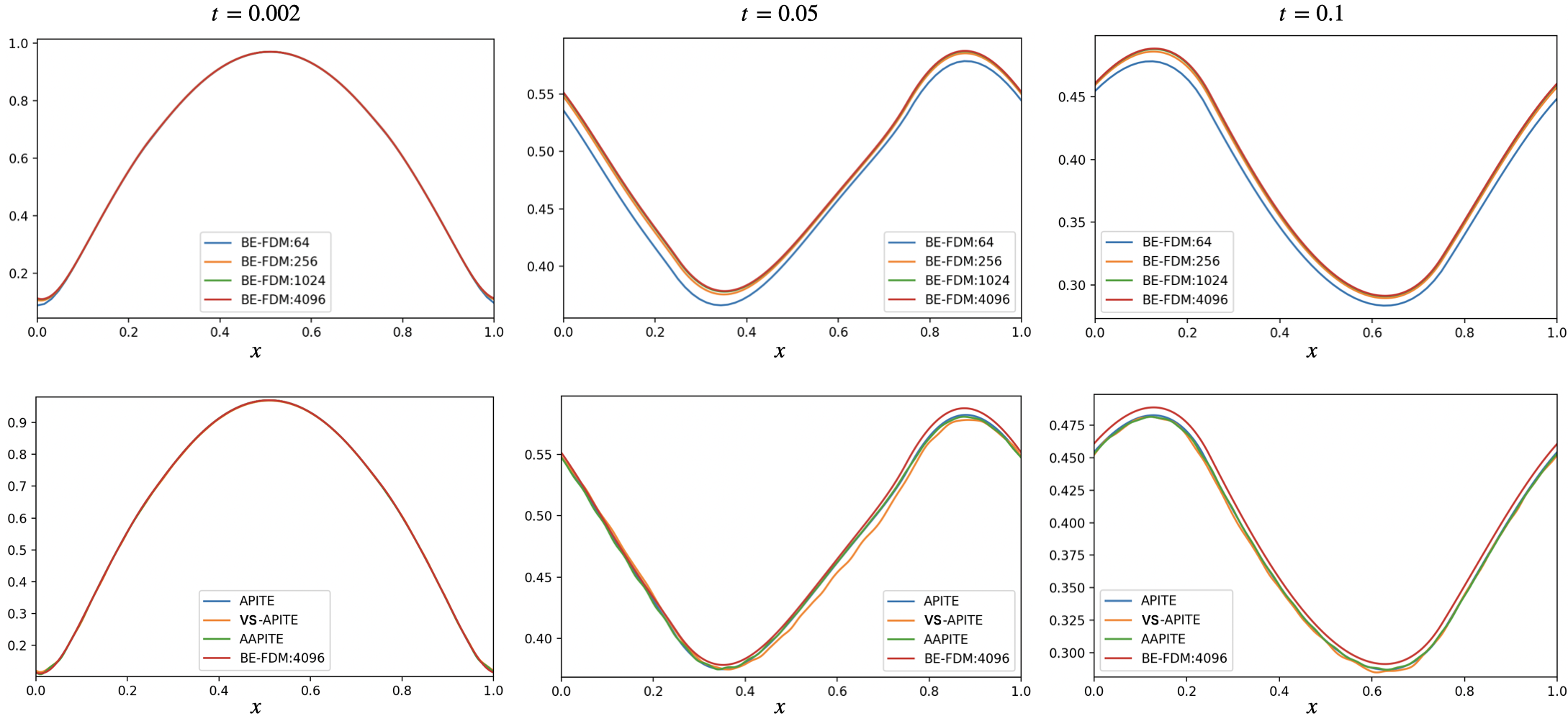
Figure 17: Plot of solutions at time $t=0.002,0.05,0.1$. In the first row, we plot the classical solutions by the backward Euler FDM with different grid parameters $N=64,256,1024,4096$. In the second row, we plot the $(2^{6},2^{8})$-quantum solutions using the approximate PITE [28] (APITE), the variable-time-step approximate PITE [29] (VS-APITE), and the alternative approximate PITE (AAPITE). A reference solution by the backward Euler FDM with large parameter $N=4096$ is also given in red. Here, the first-order Suzuki-Trotter formula is employed for the quantum solutions, and we choose the time step $\Delta\tau=0.00005$ for APITE and $\Delta\tau=0.0005$ for AAPITE, the linear-scheduled time steps $\Delta\tau_{j}\in[0.0001,0.0009]$ for VS-APITE, and the time step $\Delta\tau=t/10^{3}$ for the classical FDM solutions. Moreover, a relatively large parameter $m_{0}=0.9$ is chosen for both APITE and VS-APITE.

From the plot of the quantum solutions, we find that all the quantum solutions approximate the reference solution. As shown in the intuitive plot in Fig. 14, the original approximate PITE solution provides a good approximation for small $\Delta\tau=0.00005$, but we confirmed the numerical instability as we take a slightly larger $\Delta\tau=0.0001$ since $\Delta\tau$ should be smaller than $\pi/(2s_{0}\lambda_{N})$ by the estimation in Appendix A.1. On the contrary, the improved quantum solution with linear-scheduled varying time steps [29] taking from $\Delta\tau_{\text{min}}=0.0001$ to $\Delta\tau_{\text{max}}=0.0009$ demonstrates a normal approximation, and the alternative approximate PITE solution has already approached the reference solution with a relatively large $\Delta\tau=0.0005$. Therefore, we find that both the proposed approximate PITE and the variable-time-step approximate PITE have less restriction on $\Delta\tau$. However, the success probability of the previous approximate PITE algorithms is extremely small ($\leq 10^{-17}$ for VS-APITE and $\leq 10^{-183}$ for APITE at $t=0.1$) compared to our proposed one $(\approx 10^{-1})$, which is demonstrated in Fig. 18.

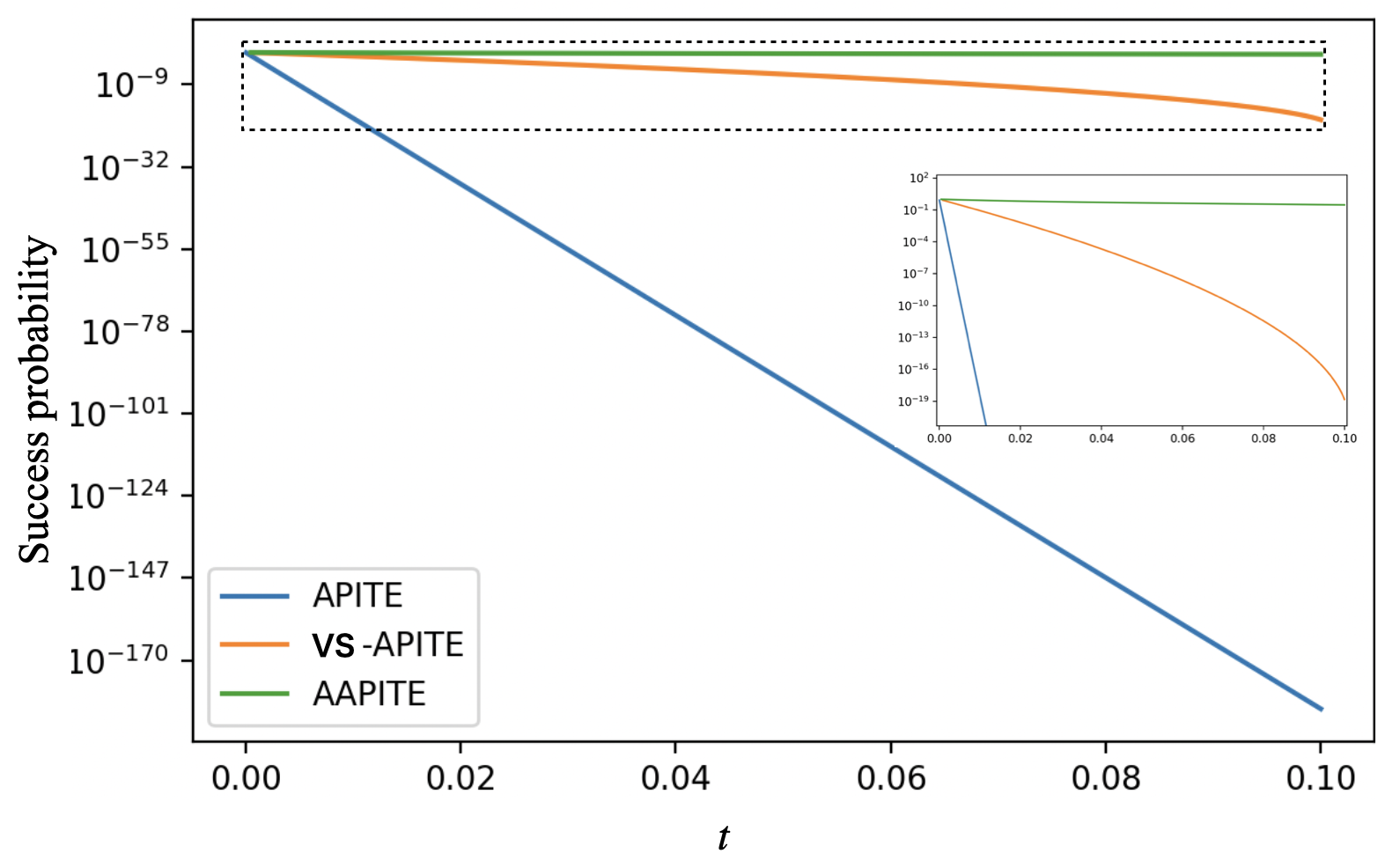
Figure 18: Success probabilities regarding simulation time $t$ for the quantum solutions by the original approximate PITE (APITE), the variable-time-step approximate PITE (VS-APITE) and the alternative approximate PITE (AAPITE). A zoom-in plot is given to show that the success probability is larger than $10^{-1}$ ($\approx 0.29889$) for AAPITE.

To provide a more quantitative comparison, we choose an exact PITE solution in a similar way as that in Sect. 4.2 as the reference solution (so that the discretization error is excluded), and we compare the $l^{2}$-errors between the quantum solutions by these three approximate PITE algorithms and the reference solution under several different choices of $\Delta\tau$ and $m_{0}$ in Fig. 19. For APITE, we find the $l^{2}$-error becomes larger for larger $m_{0}$, and actually we check that the quantum solution is unavailable due to the numerical instability if $m_{0}\geq 0.92$ and $\Delta\tau\geq 0.0001$. For VS-APITE, we find that we can choose $m_{0}=0.99$ and the minimum time step $\Delta\tau_{\text{min}}\geq 0.0001$, but larger $m_{0}$ or larger maximum time step $\Delta\tau_{\text{max}}$ leads to larger $l^{2}$-error. For AAPITE, we find that the quantum solution gives a precision of $10^{-2}$ even when we take $\Delta\tau\geq 0.0005$, and the $l^{2}$-error further decreases for smaller $\Delta\tau$. In the right subplot of Fig. 19, we confirm the crucial advantage of the alternative approximate PITE that the success probability almost remains constant whatever $\Delta\tau$ we choose. This is very important if the long-time simulations of differential equations are required.

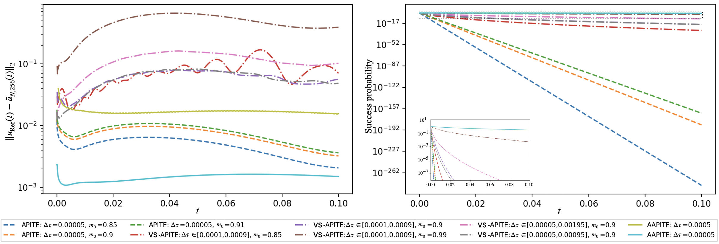
Figure 19: $l^{2}$-errors between the quantum solutions and the reference solution and corresponding success probabilities under several different choices of $\Delta\tau$ and $m_{0}$.

The time evolution of the success probabilities for the PITE algorithms are estimated theoretically in Sect. 3.2 and Appendix A.2, and we conclude the priority of the alternative approximate PITE compared to the previous ones as a quantum solver for the differential equations.

6 Extension to system of diffusion equations

We can also consider a coupled system of linear diffusion equations, which can be regarded as the linearized reaction-diffusion system. The governing equations are as follows:

$$\partial_{t}u^{(j)}(\mathbf{x},t)=a_{j}\nabla^{2}u^{(j)}(\mathbf{x},t)-\sum_{\ell=1}^{J}p_{j\ell}(\mathbf{x},t)u^{(\ell)}(\mathbf{x},t),\quad\mathbf{x}\in[0,L]^{d},\ t>0,$$ (19)

for $j=1,\ldots,J$, where $a_{j}\in\mathbb{R}_{>0}$, $j=1,\ldots,J$ are positive diffusion coefficients and $(p_{j\ell})_{j,\ell=1,\ldots,J}\in\mathbb{R}^{J\times J}$ denotes the coefficient matrix of reaction. Moreover, we include the initial conditions

$$u^{(j)}(\mathbf{x},0)=u_{0}^{(j)}(\mathbf{x}),\quad j=1,\ldots,J.$$ (20)

Let $n\in\mathbb{N}$, $N=2^{n}$, $[N]:=\{-N/2,-N/2+1,\ldots,N/2-1\}=[\tilde{N}]-N/2$, and introduce the basis $\phi_{\mathbf{k}}(\mathbf{x})=\frac{1}{L^{d/2}}e^{\mathrm{i}\frac{2\pi}{L}k_{1}x_{1}}\ldots e^{\mathrm{i}\frac{2\pi}{L}k_{d}x_{d}}$, $\mathbf{k}\in[N]^{d}$. We let the following linear combination of basis

$$u_{N}^{(j)}(\mathbf{x},t)=\sum_{\mathbf{k}\in[N]^{d}}\hat{u}_{\mathbf{k}}^{(j)}(t)\phi_{\mathbf{k}}(\mathbf{x}),$$

solve the governing equations (19) with the initial conditions

$$u_{N}^{(j)}(\mathbf{x},0)=\sum_{\mathbf{k}\in[N]^{d}}(\phi_{\mathbf{k}},u_{0}^{(j)})\phi_{\mathbf{k}}(\mathbf{x}),\quad j=1,\ldots,J,$$

which is derived from (20). By taking $\mathbf{x}=\mathbf{p}_{\mathbf{\ell}}$ (see Eq. (9)) for all $\mathbf{\ell}\in[\tilde{N}]$, we follow the discussion in Appendix B, that is, we apply the grid method to obtain a matrix equation:

$$\partial_{t}\begin{pmatrix}F_{N}&&\\ &\ddots&\\ &&F_{N}\end{pmatrix}\begin{pmatrix}\mathbf{\hat{u}}^{(1)}\\ \vdots\\ \mathbf{\hat{u}}^{(J)}\end{pmatrix}= -\begin{pmatrix}F_{N}&&\\ &\ddots&\\ &&F_{N}\end{pmatrix}\begin{pmatrix}D_{N}^{(1)}&&\\ &\ddots&\\ &&D_{N}^{(J)}\end{pmatrix}\begin{pmatrix}\mathbf{\hat{u}}^{(1)}\\ \vdots\\ \mathbf{\hat{u}}^{(J)}\end{pmatrix}$$

$$-\begin{pmatrix}P_{N}^{(11)}&\cdots&P_{N}^{(1J)}\\ \vdots&\ddots&\vdots\\ P_{N}^{(J1)}&\cdots&P_{N}^{(JJ)}\end{pmatrix}\begin{pmatrix}F_{N}&&\\ &\ddots&\\ &&F_{N}\end{pmatrix}\begin{pmatrix}\mathbf{\hat{u}}^{(1)}\\ \vdots\\ \mathbf{\hat{u}}^{(J)}\end{pmatrix},$$

where

$$\mathbf{\hat{u}}^{(j)}=\sum_{\mathbf{k}\in[\tilde{N}]^{d}}\hat{u}_{\mathbf{k}-N/2}^{(j)}(t)\left|\mathbf{k}\right\rangle,\quad j=1,\ldots,J,$$

$$D_{N}^{(j)}=\sum_{\mathbf{k}\in[\tilde{N}]^{d}}a_{j}(2\pi/L)^{2}\left|\mathbf{k}-\frac{N}{2}\right|^{2}\left|\mathbf{k}\right\rangle\left\langle\mathbf{k}\right|,\quad j=1,\ldots,J,$$

$$P_{N}^{(j\tilde{j})}(t)=\sum_{\mathbf{\ell}\in[\tilde{N}]^{d}}p_{j\tilde{j}}(\mathbf{p}_{\mathbf{\ell}},t)\left|\mathbf{\ell}\right\rangle\left\langle\mathbf{\ell}\right|=\sum_{\mathbf{\ell}\in[\tilde{N}]^{d}}p_{j\tilde{j}}\left(\frac{L}{N}\mathbf{\ell},t\right)\left|\mathbf{\ell}\right\rangle\left\langle\mathbf{\ell}\right|,\quad j,\tilde{j}=1,\ldots,J.$$

Since we intend to solve the equations on the quantum computers, we should assume $J=2^{j_{0}}$ for some integer $j_{0}\in\mathbb{N}$. Otherwise, we need to introduce some dummy equations. Henceforth, we consider the simplest case of $J=2$. Then, the above matrix equation yields

$$\partial_{t}\mathbf{y}=-\left(I\otimes F_{N}\right)\left(\left|0\right\rangle\left\langle 0\right|\otimes D_{N}^{(1)}+\left|1\right\rangle\left\langle 1\right|\otimes D_{N}^{(2)}\right)\left(I\otimes F_{N}^{\dagger}\right)\mathbf{y}-\begin{pmatrix}P_{N}^{(11)}&P_{N}^{(12)}\\ P_{N}^{(21)}&P_{N}^{(22)}\end{pmatrix}\mathbf{y}=:-H_{N}(t)\mathbf{y},$$

where $\mathbf{y}=\left(I\otimes F_{N}\right)\mathbf{\hat{u}}$ with $\mathbf{\hat{u}}=(\mathbf{\hat{u}}^{(1)};\mathbf{\hat{u}}^{(2)})$. For a given target time $T>0$, we intend to derive $\mathbf{y}(T)$. By choosing sufficiently large $K\in\mathbb{N}$ and $\Delta\tau=T/K$, we integrate the above system and obtain the approximation

$$\mathbf{y}(T)\approx\prod_{j=0}^{K-1}e^{-\Delta\tau H_{N}(j\Delta\tau)}\mathbf{y}(0),$$

with $\mathbf{y}=(\mathbf{y}^{(1)};\mathbf{y}^{(2)})$, and

$$\mathbf{y}^{(j)}(0)=\frac{1}{N^{d/2}}\sum_{\mathbf{\ell}\in[\tilde{N}]^{2}}\left(\sum_{\mathbf{k}\in[N]^{2}}(\phi_{\mathbf{k}},u_{0}^{(j)})e^{\mathrm{i}\frac{2\pi}{N}\mathbf{k}\cdot\mathbf{\ell}}\right)\left|\mathbf{\ell}\right\rangle\approx\left(\frac{L}{N}\right)^{d/2}\sum_{\mathbf{\ell}\in[\tilde{N}]^{2}}u_{0}^{(j)}(\mathbf{x}_{\mathbf{\ell}})\left|\mathbf{\ell}\right\rangle,\quad j=1,2.$$

Now, we are interested in the ITE operator $e^{-\Delta\tau H_{N}(j\Delta\tau)}$ for each $j=0,\ldots,K-1$. By the first-order Suzuki-Trotter formula, we have

$$e^{-\Delta\tau H_{N}(j\Delta\tau)} \approx e^{-\Delta\tau\left(I\otimes F_{N}\right)\left(\left|0\right\rangle\left\langle 0\right|\otimes D_{N}^{(1)}+\left|1\right\rangle\left\langle 1\right|\otimes D_{N}^{(2)}\right)\left(I\otimes F_{N}^{\dagger}\right)}e^{-\Delta\tau\left(\left|0\right\rangle\left\langle 0\right|\otimes P_{N}^{(11)}(j\Delta\tau)+\left|1\right\rangle\left\langle 1\right|\otimes P_{N}^{(22)}(j\Delta\tau)\right)}$$

$$\quad e^{-\frac{1}{2}\Delta\tau X\otimes\left(P_{N}^{(12)}(j\Delta\tau)+P_{N}^{(21)}(j\Delta\tau)\right)}e^{-\frac{1}{2}\mathrm{i}\Delta\tau Y\otimes\left(P_{N}^{(12)}(j\Delta\tau)-P_{N}^{(21)}(j\Delta\tau)\right)}.$$

Here and henceforth, $X$, $Y$, and $Z$ denote Pauli matrices. More precisely, we rewrite the four operations as follows:

$$e^{-\Delta\tau\left(I\otimes F_{N}\right)\left(\left|0\right\rangle\left\langle 0\right|\otimes D_{N}^{(1)}+\left|1\right\rangle\left\langle 1\right|\otimes D_{N}^{(2)}\right)\left(I\otimes F_{N}^{\dagger}\right)} =\left(\left|0\right\rangle\left\langle 0\right|\otimes e^{-\Delta\tau F_{N}D_{N}^{(1)}F_{N}^{\dagger}}\right)+\left(\left|1\right\rangle\left\langle 1\right|\otimes e^{-\Delta\tau F_{N}D_{N}^{(2)}F_{N}^{\dagger}}\right)$$

$$=(I\otimes F_{N})e^{-\Delta\tau\left(\left|0\right\rangle\left\langle 0\right|\otimes D_{N}^{(1)}+\left|1\right\rangle\left\langle 1\right|\otimes D_{N}^{(2)}\right)}(I\otimes F_{N}^{\dagger}),$$

$$e^{-\Delta\tau\left(\left|0\right\rangle\left\langle 0\right|\otimes P_{N}^{(11)}(j\Delta\tau)+\left|1\right\rangle\left\langle 1\right|\otimes P_{N}^{(22)}(j\Delta\tau)\right)} =e^{\Delta\tau P_{0}}e^{-\Delta\tau\left(\left|0\right\rangle\left\langle 0\right|\otimes P_{N}^{(11)}(j\Delta\tau)+\left|1\right\rangle\left\langle 1\right|\otimes P_{N}^{(22)}(j\Delta\tau)+P_{0}I\right)},$$

$$e^{-\frac{1}{2}\Delta\tau X\otimes\left(P_{N}^{(12)}(j\Delta\tau)+P_{N}^{(21)}(j\Delta\tau)\right)} =(H\otimes I)e^{-\frac{1}{2}\Delta\tau Z\otimes\left(P_{N}^{(12)}(j\Delta\tau)+P_{N}^{(21)}(j\Delta\tau)\right)}(H\otimes I)$$

$$=e^{\frac{1}{2}\Delta\tau P_{1}}(H\otimes I)e^{-\frac{1}{2}\Delta\tau\left(Z\otimes\left(P_{N}^{(12)}(j\Delta\tau)+P_{N}^{(21)}(j\Delta\tau)\right)+P_{1}I\right)}(H\otimes I),$$

$$e^{-\frac{1}{2}\mathrm{i}\Delta\tau Y\otimes\left(P_{N}^{(12)}(j\Delta\tau)-P_{N}^{(21)}(j\Delta\tau)\right)}=(W\otimes I)e^{-\frac{1}{2}\mathrm{i}\Delta\tau Z\otimes\left(P_{N}^{(12)}(j\Delta\tau)-P_{N}^{(21)}(j\Delta\tau)\right)}(W^{\dagger}\otimes I),$$

where

$$P_{0}(j\Delta\tau) =-\min\left\{\min_{\mathbf{x}\in[0,L]^{2}}p_{11}(\mathbf{x},j\Delta\tau),\min_{\mathbf{x}\in[0,L]^{2}}p_{22}(\mathbf{x},j\Delta\tau)\right\},$$

$$P_{1}(j\Delta\tau) =\max_{\mathbf{x}\in[0,L]^{2}}\left|p_{12}(\mathbf{x},j\Delta\tau)+p_{21}(\mathbf{x},j\Delta\tau)\right|,$$

and

$$H=\frac{1}{\sqrt{2}}\begin{pmatrix}1&1\\ 1&-1\end{pmatrix},\quad W=\frac{1}{\sqrt{2}}\begin{pmatrix}1&\mathrm{i}\\ \mathrm{i}&1\end{pmatrix}=R_{x}(-\pi/2).$$

Recalling that $D_{N}^{(j)}$, $j=1,2$ and $P_{N}^{(j\tilde{j})}$, $j,\tilde{j}=1,2$ are both diagonal matrices. The above calculations imply

$$e^{-\Delta\tau H_{N}(j\Delta\tau)} \approx e^{\Delta\tau(P_{0}+P_{1}/2)}(I\otimes F_{N})e^{-D_{1}}(I\otimes F_{N}^{\dagger})e^{-D_{2}}(H\otimes I)e^{-D_{3}}(HW\otimes I)e^{-\mathrm{i}D_{4}}(W^{\dagger}\otimes I),$$

where $D_{1},D_{2},D_{3}$ and $D_{4}$ are all diagonal matrices with non-negative entries. Therefore, we can apply the proposed approximate PITE operator for three times and a RTE operator once, all for real-valued diagonal matrices, to approximately implement the imaginary-time operator in each time step. The quantum circuit in one time step is demonstrated in Fig. 20.

Figure 20: A quantum circuit of one time step for solving a system of diffusion equations using the alternative approximate PITE. Here, three approximate PITE circuits are employed. The first one is for the diffusion, and the rest two are for the diagonal components and the symmetric part of the non-diagonal components of the reaction matrix, respectively.

If we are able to retrieve the solutions after each time step by measurements, then we can employ the solutions to construct the Hamiltonian in the next time step, which means we can deal with the nonlinear reaction-diffusion equations. For example, let $J=2$ in Eq. (19) and we have

$$\partial_{t}u^{(1)}(\mathbf{x},t)=a_{1}\nabla^{2}u^{(1)}(\mathbf{x},t)-p_{11}(\mathbf{x},t)u^{(1)}(\mathbf{x},t)-p_{12}(\mathbf{x},t)u^{(2)}(\mathbf{x},t),\quad\mathbf{x}\in[0,L]^{d},\ t>0,$$

$$\partial_{t}u^{(2)}(\mathbf{x},t)=a_{2}\nabla^{2}u^{(2)}(\mathbf{x},t)-p_{21}(\mathbf{x},t)u^{(1)}(\mathbf{x},t)-p_{22}(\mathbf{x},t)u^{(2)}(\mathbf{x},t),\quad\mathbf{x}\in[0,L]^{d},\ t>0.$$

Let $p_{ij}$, $i,j=1,2$ be some functions of $u^{(1)}$ and $u^{(2)}$. Then, we obtain the nonlinear reaction-diffusion equations. In the following context, we discuss two examples.

Example 1 Turing Pattern formulation

Let $a_{1}=0.005$, $a_{2}=0.1$, $L=2\pi$, $p_{11}=(u^{(1)})^{2}-0.6$, $p_{12}=1$, $p_{21}=-1.5$, $p_{22}=2$. We consider the initial conditions of four point sources described by the linear combination of the Gaussian functions:

$$u_{0}^{(1)}(\mathbf{x})=u_{0}^{(2)}(\mathbf{x})=A\sum_{j=1}^{4}\mathrm{exp}\left(-\frac{|\mathbf{x}-\mathbf{x}_{0}^{(j)}|^{2}}{2\sigma^{2}}\right).$$

Here, $\sigma^{2}=0.05$, $\mathbf{x}_{0}^{(1)}=(\pi/2,\pi/2)^{\mathrm{T}}$, $\mathbf{x}_{0}^{(2)}=(\pi/2,3\pi/2)^{\mathrm{T}}$, $\mathbf{x}_{0}^{(3)}=(3\pi/2,\pi/2)^{\mathrm{T}}$, $\mathbf{x}_{0}^{(4)}=(3\pi/2,3\pi/2)^{\mathrm{T}}$, and $A$ is a normalized parameter such that the $l^{2}$ norm of the function at $N^{2}$ grid points is normalized to $1$. We provide a simulation result with $N=2^{4}$ in Fig. 21.

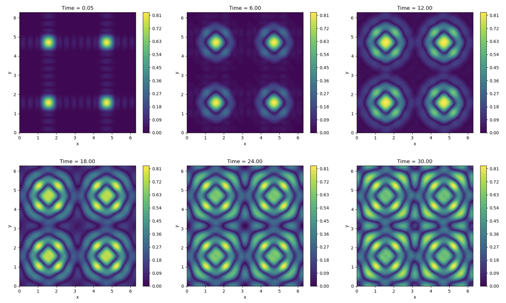
Figure 21: Time evolution of the $(2^{4},2^{7})$-quantum solution using the alternative approximate PITE operator with $\Delta\tau=0.05$ for the first component of a reaction-diffusion system. The quantum solutions at $t=0.05,6,12,18,24,30$ are visualized using colormap plots. In each subplot, the $x$ and $y$ axes describe the location in $x_{1}$-direction and $x_{2}$-direction, respectively.

It demonstrates the formulation of ring pattern around the initial point sources. The simulation is done by Qiskit emulator, and we directly obtain the success probability by the state vector after each PITE step. In this example, the total success probability is extremely small ($\approx 10^{-21}$).

Example 2 Burgers’ equation

Let $a_{1}=0.05$, $a_{2}=0.05$, $L=2\pi$, $p_{11}=\partial_{x_{1}}u^{(1)}$, $p_{12}=\partial_{x_{2}}u^{(1)}$, $p_{21}=\partial_{x_{1}}u^{(2)}$, $p_{22}=\partial_{x_{2}}u^{(2)}$. Then, Eq. (19) becomes (viscous) Burgers’ equation with viscosity $\nu=0.05$:

$$\partial_{t}\mathbf{u}(\mathbf{x},t)=\nu\nabla^{2}\mathbf{u}(\mathbf{x},t)-\mathbf{u}\cdot\nabla\mathbf{u}(\mathbf{x},t),\quad\mathbf{x}\in[0,L],\ t>0.$$

Here, the spatial derivatives of the solutions are calculated from the solutions using the fast Fourier transform on a classical computer. As a simple numerical example, we consider the initial conditions:

$$u_{0}^{(1)}(x_{1},x_{2})=\sin(2x_{1}), x_{1},x_{2}\in[0,2\pi],$$

$$u_{0}^{(2)}(x_{1},x_{2})=0.5, x_{1},x_{2}\in[0,2\pi].$$

Under these initial conditions, the 2D Burgers’ equation reduces to a 1D Burgers’ equation, and the simulation result is shown in Fig. 22.

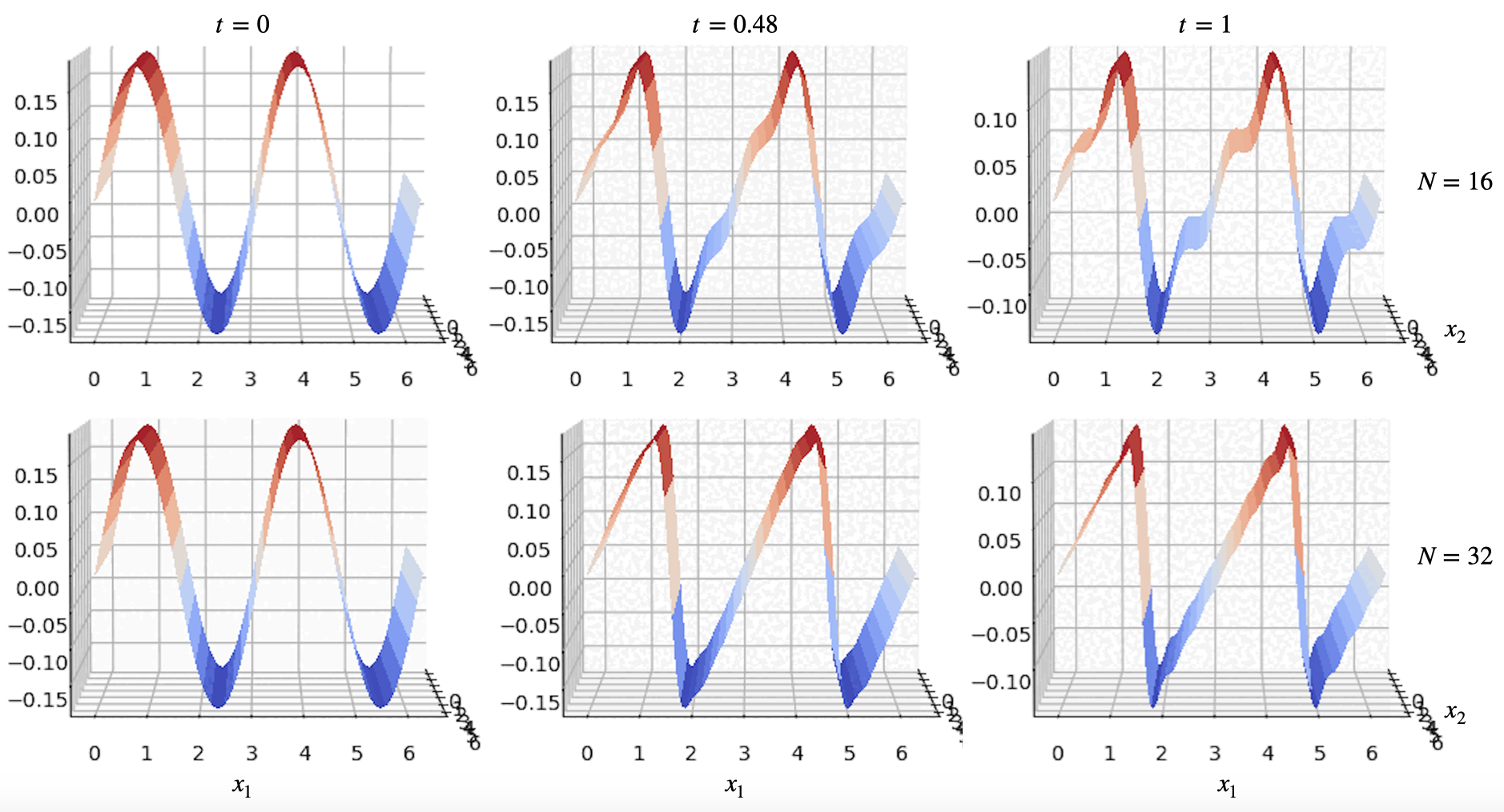
Figure 22: Time evolution of the $(N,2^{7})$-quantum solution using the alternative approximate PITE operator with $\Delta\tau=0.04$ for the first component of Burgers’ equation. The quantum solutions at $t=0,0.48,1$ are visualized using 3D plots from left to right. We take $N=2^{4}=16$ in the first row and $N=2^{5}=32$ in the second row. Despite of $N=16$ or $N=32$, the success probability is about $2\times 10^{-4}$.

We find that the initial sine wave becomes a sawtooth wave as time goes by. Moreover, the quantum solution has better performance for a larger grid parameter $N$ as we observe less numerical oscillation in the $(2^{5},2^{7})$-quantum solution than that in the $(2^{4},2^{7})$-quantum solution.

The success probability is about $2\times 10^{-4}$, which is relatively large compared to the extremely small success probability in the previous example. This implies nonlinearity does not necessarily lead to a small success probability. By the theoretical analysis in Sect. 3.2, we find the success probability mainly depends on the change of the $L^{2}$-norm of the solution compared to the initial condition. Therefore, quantum solvers may be more expensive (large number of repetitions and measurements) than their classical counterparts in the simulations of highly dissipative systems, whatever they are linear or nonlinear.

In the simulation of Burgers’ equation, a further observation is that smaller viscosity $\nu$ yields severer numerical oscillation (this is also a crucial problem in the classical simulations), and hence, we have to take larger grid parameter $N$ and smaller time step $\Delta\tau$ to relieve the oscillation.

7 Summary and concluding remarks

In this paper, we discuss a new approximate PITE and its application to solving the time evolution differential equations using examples of the advection-diffusion equations.

First, we proposed an alternative approximate PITE operator, which approximates the ITE operator $m_{0}e^{-\Delta\tau\mathcal{H}}$ with $m_{0}=1$. We obtained analytical estimations for both the $l^{2}$-error and its success probability. Compared to the original approximate PITE in [28] where $m_{0}$ is strictly smaller than one, the alternative approximate PITE relieves the restriction in the time step $\Delta\tau$. Moreover, it avoids the problem of the rapid vanishing of the success probability (see Sect. 2.3 and Appendix A.2). For the convenience of applications, the $l^{2}$-error and the success probability in the case of the Hamiltonian coming from the advection-diffusion equations were also estimated.

Second, as for the gate implementation of the alternative approximate PITE, we need to employ the RTE operator for the squared root Hamiltonian, that is, $U_{\text{RTE}}(\sqrt{2\Delta\tau\mathcal{H}})$. Although the squared root Hamiltonian is usually more complicated than the original one in general, one can use the general Hamiltonian simulation techniques in e.g., [44, 13]. In this paper, for the advection-diffusion equation, we provided an explicit gate implementation for the RTE of the discretized Hamiltonian matrix based on the grid method using the efficient quantum circuits for the diagonal unitary matrices [37, 31]. Applying the techniques in [31], we can implement the alternative approximate PITE operator by $O(\mathrm{poly}\,n)$ two-qubit gates with only $2$ ancillary qubits (one for the approximate PITE and the other for the diagonal unitary matrices) in 1D cases and $2n+2+\lceil\log_{2}d\rceil$ ancillary qubits (another $2n+\lceil\log_{2}d\rceil$ qubits for the distance register) in multi-dimensional cases. The required number of ancillary qubits is the least one among all the quantum algorithms to our best knowledge.

Third, we provided 1D/2D numerical examples for solving the advection-diffusion-reaction equations by the alternative approximate PITE. The simulations were executed by Qiskit (a quantum gate-based emulator). The numerical results demonstrated good agreement with the true solutions. Moreover, based on the mathematical theory for the grid method (Appendix B), we suggested pre-processing/post-processing steps on classical computers to improve the precision or derive the solutions on a finer mesh when the (quantum) computational grid is relatively small due to the limited capacity of the near-term quantum computers. Furthermore, we divided the error into the discretization error, the Suzuki-Trotter error and the (PITE) approximation error, and confirmed the important dependence on the grid parameter $N$ and the time step $\Delta\tau$ numerically, which coincides with the theoretical estimations.

Fourth, we compared our algorithm based on the alternative approximate PITE with the ones in the previous works [28, 29]. The result implies that the original approximate PITE [28] and even the improved version [29] with varying time steps are not suitable for the task of solving differential equations since they undergo the rapid decrease of the success probability owing to $m_{0}<1$. On the other hand, we also compared the alternative approximate PITE with the HHL algorithm and concluded that our proposed approximate PITE uses much less ancillary qubits while the performances are comparable. Besides, we used the comparison with a previous work on the advection-diffusion equation to address that our quantum algorithm based on the grid method (a specific FSM) outperforms the HHL algorithms using the sparse discretized matrices by the FDMs. If the boundary condition is not important or is periodic, then the discretization based on the FSM is recommended because it has better precision than many other discretization methods (FDM, FEMs, etc.) as $N$ increases and can be explicitly and efficiently implemented on quantum computers. Furthermore, our proposed approximate PITE circuit can also be applied to other discretized matrices deriving from the FDMs, FEMs, etc. In such cases, we need a subroutine implementing the RTE operator for the discretized Hamiltonian, which is possible by the general techniques in [44, 13] using more ancillary qubits.

Finally, we extended our algorithm to the (linearized) diffusion-reaction systems. For the quantum algorithm, we need only $dn\log_{2}J$ qubits to simulate the system consisted of $J$ equations, which seems more efficient than its classical counterpart. In the simplest case of $J=2$, we provided the detailed implementation of the system using three PITE operators in one time step. Moreover, if we allow the measurement of the solution after each time step, we can apply such information to update the Hamiltonian in the next time step, so that nonlinear systems can be treated. Simulations of Turing Pattern formulation and Burgers’ equation were provided for potential applications if efficient statevector preparation/readout techniques would be developed in the future.

One future topic is the application to the problem of ground state/eigenstate preparation. We know that the ITE operator of a given Hamiltonian $\mathcal{H}$ is useful in deriving its ground state since the overlaps regarding the excited states tend to zero exponentially as the time-like parameter increases. Different from solving the numerical solutions to differential equations, for the ground state preparation problem, the evolution of the excited states is not necessarily to be exactly an exponential decrease, and hence, one can use an energy shift technique to avoid the rapid decay of the success probability [29, 37] in the original approximate PITE. Although, the alternative approximate PITE definitely applies for such a problem, it remains open whether the alternative approximate PITE outperforms the original approximate PITE [28] and its derivative [29] in this case.

Another future work is the insight comparisons to other quantum algorithms. One is the improved QLSAs based on Fourier(-like) method in [15] and Sect. 4 in [16]. The theoretical overheads of the query complexity and the gate complexity were established, but the detailed implementations for the Hamiltonian simulation of the discretized matrices are not clear. Despite of the polynomial order $O(\mathrm{poly}\,n)$ of the gate complexity, the pre-factor seems large using the techniques mentioned therein. Another interesting one is the recently proposed Schrödingerisation method [24, 25]. According to [25], the discretization methods based on both the FDMs and the Fourier method can be considered in their framework. Although their algorithm needs additional ancillary qubits for the augmented matrix, it seems that the success probability may be independent of the norm change in the specific case that we seek only the normalized solution. Therefore, more insight discussions and comparison are indispensable to find which is the best quantum solver for the linear differential equations or whether we should choose a suitable one for each discrete scenario.

Appendix A Approximate PITE [Kosugi et al. 2022]

We provide detailed analysis for an approximate PITE that is equivalent to the one in [28]. Take $\Theta:=\arccos(m_{0}e^{-\Delta\tau\mathcal{H}})$ with an arbitrarily fixed parameter $m_{0}\in(0,1)$. We denote the real-valued function $g_{0}(x):=\arccos(m_{0}e^{-x})$, $x\geq 0$. By the Taylor expansion around $x_{0}\geq 0$ up to first order, we obtain

$$g_{0}(x)=g_{0}(x_{0})+g_{0}^{\prime}(x_{0})(x-x_{0})+O(|x-x_{0}|^{2}).$$

By noting

$$\lim_{x\to 0}g_{0}(x)=\arccos(m_{0})=:\theta_{0},\quad\lim_{x\to 0}g_{0}^{\prime}(x)=\lim_{x\to 0}\frac{m_{0}e^{-x}}{\sqrt{1-(m_{0}e^{-x})^{2}}}=\frac{m_{0}}{\sqrt{1-m_{0}^{2}}}=:s_{0},$$

and taking $x_{0}=0$, we reach the approximation

$$\Theta=g_{0}(\Delta\tau\mathcal{H})=\theta_{0}I+s_{0}\Delta\tau\mathcal{H}+O((\Delta\tau)^{2})\approx\theta_{0}I+s_{0}\Delta\tau\mathcal{H}.$$

In other words,

$$m_{0}e^{-\Delta\tau\mathcal{H}}=\cos(g_{0}(\Delta\tau\mathcal{H}))\approx\cos(\theta_{0}I+s_{0}\Delta\tau\mathcal{H}).$$

Here, we mention that $m_{0}\not=1$, otherwise, the above Taylor expansion does not converge. Since

$$U_{\text{RTE}}(\pm(\theta_{0}I+s_{0}\Delta\tau\mathcal{H}))=U_{\text{RTE}}(\pm\theta_{0}I)U_{\text{RTE}}(\pm s_{0}\Delta\tau\mathcal{H}),$$

and the four RTE operators $U_{\text{RTE}}(\pm\theta_{0}I)$, $U_{\text{RTE}}(\pm s_{0}\Delta\tau\mathcal{H})$ are commutable, from Fig. 1, we obtain the quantum circuit in Fig. 23, in which we used the relation

$$e^{\mathrm{i}\theta_{0}}\left|0\right\rangle\left\langle 0\right|+e^{-\mathrm{i}\theta_{0}}\left|1\right\rangle\left\langle 1\right|=R_{z}(-2\theta_{0}).$$

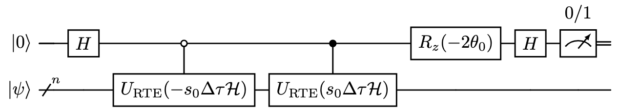
Figure 23: A quantum circuit for approximate PITE. This quantum circuit is equivalent to Fig. 1(b) in [28].

In the sense of possibly applying two single-qubit gates $Q$ and $Q^{\dagger}$ to the ancillary qubit, the proposed circuit in Fig. 23 is equivalent to Fig. 1(b) in [28].

Before the estimations of the error and the success probability, we mention the quantum resources used in a single PITE step. By the construction, it is clear that the main request of quantum resources comes from the part of controlled RTE operator of a given Hermite operator $\mathcal{H}$. In the practical applications in the first-quantized formulation, admitting the error from the Suzuki-Trotter expansion, it is well-known that such controlled RTE operators can be implemented efficiently in gate complexity $O(\mathrm{poly}\log N)$ (e.g., [28]). In the dependence of $N$, this is an exponential improvement compared to the exact implementation mentioned in Sect. 2.

A.1 Error estimate

For simplicity, we consider a $K$-step approximate PITE for $K\in\mathbb{N}$, and we assume that the eigenvalues of $\mathcal{H}$: $\{\lambda_{k}\}_{k=0}^{N-1}$ are non-negative without loss of generality. As long as we know the smallest eigenvalue of $\mathcal{H}$: $\lambda_{min}$, we can shift the operator $\mathcal{H}$ by $\lambda_{\ast}I$ for any $\lambda_{\ast}\leq\lambda_{min}$ and consider the shifted operator $\widetilde{\mathcal{H}}:=\mathcal{H}-\lambda_{\ast}I$. Thus,

$$e^{-\Delta\tau\mathcal{H}}=e^{-\Delta\tau\lambda_{\ast}}e^{-\Delta\tau\widetilde{\mathcal{H}}},$$

and we can moreover assume that the smallest eigenvalue of the shifted operator is exactly zero, provided that we know exactly the smallest eigenvalue of the original operator $\mathcal{H}$.

For an approximate PITE circuit, of course, we have error due to the approximation. We introduce the error after normalization, which is defined by

$$\mathrm{Err}_{2}:=\left\|\frac{\cos^{K}(\theta_{0}+s_{0}\Delta\tau\mathcal{H})\left|\psi\right\rangle}{\|\cos^{K}(\theta_{0}+s_{0}\Delta\tau\mathcal{H})\left|\psi\right\rangle\|}-\frac{e^{-K\Delta\tau\mathcal{H}}\left|\psi\right\rangle}{\|e^{-K\Delta\tau\mathcal{H}}\left|\psi\right\rangle\|}\right\|,$$

where $\left|\psi\right\rangle$ is an initial state. Moreover, we estimate by the triangle inequalities $|\|a\|-\|b\||\leq\|a-b\|\leq\|a\|+\|b\|$ that

$$\mathrm{Err}_{2} \leq\left\|\frac{\cos^{K}(\theta_{0}+s_{0}\Delta\tau\mathcal{H})\left|\psi\right\rangle}{\|\cos^{K}(\theta_{0}+s_{0}\Delta\tau\mathcal{H})\left|\psi\right\rangle\|}-\frac{m_{0}^{K}e^{-K\Delta\tau\mathcal{H}}\left|\psi\right\rangle}{\|\cos^{K}(\theta_{0}+s_{0}\Delta\tau\mathcal{H})\left|\psi\right\rangle\|}\right\|$$

$$\quad+\left\|\frac{m_{0}^{K}e^{-K\Delta\tau\mathcal{H}}\left|\psi\right\rangle}{\|\cos^{K}(\theta_{0}+s_{0}\Delta\tau\mathcal{H})\left|\psi\right\rangle\|}-\frac{e^{-K\Delta\tau\mathcal{H}}\left|\psi\right\rangle}{\|e^{-K\Delta\tau\mathcal{H}}\left|\psi\right\rangle\|}\right\|$$

$$\leq 2\frac{\|\cos^{K}(\theta_{0}+s_{0}\Delta\tau\mathcal{H})\left|\psi\right\rangle-m_{0}^{K}e^{-K\Delta\tau\mathcal{H}}\left|\psi\right\rangle\|}{\|\cos^{K}(\theta_{0}+s_{0}\Delta\tau\mathcal{H})\left|\psi\right\rangle\|}.$$

The denominator is the square root of the success probability:

$$\mathbb{P}_{2}(\left|0\right\rangle):=\|\cos^{K}(\theta_{0}+s_{0}\Delta\tau\mathcal{H})\left|\psi\right\rangle\|^{2}.$$

If we denote the numerator by

$$\widetilde{\mathrm{Err}_{2}}:=\|\cos^{K}(\theta_{0}+s_{0}\Delta\tau\mathcal{H})\left|\psi\right\rangle-m_{0}^{K}e^{-K\Delta\tau\mathcal{H}}\left|\psi\right\rangle\|,$$

then again by the triangle inequalities, we obtain

$$\|m_{0}^{K}e^{-K\Delta\tau\mathcal{H}}\left|\psi\right\rangle\|-\widetilde{\mathrm{Err}_{2}}\leq\|\cos^{K}(\theta_{0}+s_{0}\Delta\tau\mathcal{H})\left|\psi\right\rangle\|\leq\|m_{0}^{K}e^{-K\Delta\tau\mathcal{H}}\left|\psi\right\rangle\|+\widetilde{\mathrm{Err}_{2}}.$$ (21)

Thus, we find that the denominator goes to $m_{0}^{K}\|e^{-K\Delta\tau\mathcal{H}}\left|\psi\right\rangle\|$ as $\widetilde{\mathrm{Err}_{2}}\to 0$, and hence the success probability

$$\mathbb{P}_{2}(\left|0\right\rangle)\to m_{0}^{2K}\|e^{-K\Delta\tau\mathcal{H}}\left|\psi\right\rangle\|^{2}\quad\text{as }\ \widetilde{\mathrm{Err}_{2}}\to 0.$$

Therefore, it is essential to estimate the upper bound of the numerator $\widetilde{\mathrm{Err}_{2}}$. Here, we adapt the non-decreasing ordering $\lambda_{0}\leq\lambda_{1}\leq\cdots\leq\lambda_{N-1}$ of the eigenvalues, and we denote the corresponding eigenfunctions by $\{\psi_{k}\}_{k=0}^{N-1}$, which forms a complete orthonormal basis of $\mathbb{C}^{N}$. Recall that $N_{\delta}(\psi)$ and $\mathcal{K}_{\delta}(\psi)$ are defined by Eqs. (1) and (2), respectively. Then, we can calculate

$$\quad\left\|\cos^{K}(\theta_{0}+s_{0}\Delta\tau\mathcal{H})\left|\psi\right\rangle-m_{0}^{K}e^{-K\Delta\tau\mathcal{H}}\left|\psi\right\rangle\right\|^{2}$$

$$=\sum_{k=0}^{N-1}|\langle\psi_{k}|\psi\rangle|^{2}\left|\cos^{K}(\theta_{0}+s_{0}\Delta\tau\lambda_{k})-(m_{0}e^{-\Delta\tau\lambda_{k}})^{K}\right|^{2}$$

$$=m_{0}^{2K}\left(\sum_{k\in\mathcal{K}_{\delta}}+\sum_{k\in[\tilde{N}]\setminus\mathcal{K}_{\delta}}\right)|\langle\psi_{k}|\psi\rangle|^{2}\left|(\cos(\theta_{0}+s_{0}\Delta\tau\lambda_{k})/m_{0})^{K}-(e^{-\Delta\tau\lambda_{k}})^{K}\right|^{2}$$

$$\leq m_{0}^{2K}\left(\sum_{k\in\mathcal{K}_{\delta}}|\langle\psi_{k}|\psi\rangle|^{2}\left|(\cos(\theta_{0}+s_{0}\Delta\tau\lambda_{k})/m_{0}-e^{-\Delta\tau\lambda_{k}})\left(\sum_{j=0}^{K-1}(\cos(\theta_{0}+s_{0}\Delta\tau\lambda_{k})/m_{0})^{j}(e^{-\Delta\tau\lambda_{k}})^{K-1-j}\right)\right|^{2}+4\delta\right)$$

$$\leq m_{0}^{2K}\left(\sum_{k\in\mathcal{K}_{\delta}}|\langle\psi_{k}|\psi\rangle|^{2}\left|\cos(\theta_{0}+s_{0}\Delta\tau\lambda_{k})/m_{0}-e^{-\Delta\tau\lambda_{k}}\right|^{2}\left(\sum_{j=0}^{K-1}|\cos(\theta_{0}+s_{0}\Delta\tau\lambda_{k})/m_{0}|^{j}|e^{-\Delta\tau\lambda_{k}}|^{K-1-j}\right)^{2}+4\delta\right)$$

$$\leq m_{0}^{2K}\left(K^{2}\sum_{k\in\mathcal{K}_{\delta}}|\langle\psi_{k}|\psi\rangle|^{2}\left|\cos(\theta_{0}+s_{0}\Delta\tau\lambda_{k})/m_{0}-e^{-\Delta\tau\lambda_{k}}\right|^{2}+4\delta\right)$$

$$=m_{0}^{2K}\left(K^{2}\sum_{k\in\mathcal{K}_{\delta}}|\langle\psi_{k}|\psi\rangle|^{2}\left|\cos(s_{0}\Delta\tau\lambda_{k})-m_{0}^{-1}\sqrt{1-m_{0}^{2}}\sin(s_{0}\Delta\tau\lambda_{k})-e^{-\Delta\tau\lambda_{k}}\right|^{2}+4\delta\right).$$

Here, in the second last line, we used an assumption that $\Delta\tau$ is small enough such that $s_{0}\Delta\tau\lambda_{N_{\delta}}\in[0,\pi/2]$, which indicates a restriction

$$|\cos(\theta_{0}+s_{0}\Delta\tau\lambda_{k})/m_{0}|=\left|\cos(s_{0}\Delta\tau\lambda_{k})-\frac{\sqrt{1-m_{0}^{2}}}{m_{0}}\sin(s_{0}\Delta\tau\lambda_{k})\right|\leq 1,\quad\text{for all }k=0,\ldots,N_{\delta}.$$

Moreover, in the first inequality, we actually used an assumption that $|\cos(\theta_{0}+s\Delta\tau\lambda_{k})/m_{0}|\leq 1$ for $k\in[\tilde{N}]\setminus\mathcal{K}_{\delta}$. Such an assumption yields a hidden constraint among the choices of $m_{0}$, $\Delta\tau$ and the spectrum of the Hermite operator. Note that the trigonometric functions and the exponential functions are smooth in $\mathbb{R}$. By employing the Taylor’s theorem with the Lagrange form of the remainder, we obtain

$$\quad\cos(s_{0}\Delta\tau\lambda_{k})-\frac{\sqrt{1-m_{0}^{2}}}{m_{0}}\sin(s_{0}\Delta\tau\lambda_{k})-e^{-\Delta\tau\lambda_{k}}$$

$$=\lambda_{k}^{2}(\Delta\tau)^{2}\left(-s_{0}^{2}\cos(s_{0}\lambda_{k}\xi)+s_{0}\sin(s_{0}\lambda_{k}\xi)-e^{-\lambda_{k}\xi}\right)/2,$$

for some $0\leq\xi\leq\Delta\tau$. Therefore, we obtain

$$\quad\left\|\cos^{K}(\theta_{0}+s_{0}\Delta\tau\mathcal{H})\left|\psi\right\rangle-m_{0}^{K}e^{-K\Delta\tau\mathcal{H}}\left|\psi\right\rangle\right\|^{2}\leq m_{0}^{2K}\left(\left(\frac{K(s_{0}^{2}+1)(\Delta\tau)^{2}}{2}\right)^{2}\sum_{k\in\mathcal{K}_{\delta}}\lambda_{k}^{4}|\langle\psi_{k}|\psi\rangle|^{2}+4\delta\right).$$

Here, we used that $\cos(s_{0}\lambda_{k}\xi),\sin(s_{0}\lambda_{k}\xi)>0$ and $\sin(s_{0}\lambda_{k}\xi)$ is close to zero for all $k=0,\ldots,N_{\delta}$. By setting $T=K\Delta\tau$ and denoting

$$C_{m_{0}}(\left|\psi\right\rangle,\delta):=(1-m_{0}^{2})^{-1}\left(\sum_{k\in\mathcal{K}_{\delta}}\lambda_{k}^{4}|\langle\psi_{k}|\psi\rangle|^{2}\right)^{1/2},$$

we reach the estimate

$$\mathrm{Err}_{2}\leq m_{0}^{K}(C_{m_{0}}(\left|\psi\right\rangle,\delta)T\Delta\tau+4\sqrt{\delta})/\sqrt{\mathbb{P}_{2}(\left|0\right\rangle)}\leq m_{0}^{K}\left((1-m_{0}^{2})^{-1}\lambda_{N_{\delta}}^{2}T\Delta\tau+4\sqrt{\delta}\right)/\sqrt{\mathbb{P}_{2}(\left|0\right\rangle)},$$ (22)

for any $\delta\in[0,1)$. By Eq. (21), we have

$$\mathrm{Err}_{2}\leq\frac{(1-m_{0}^{2})^{-1}\lambda_{N_{\delta}}^{2}T\Delta\tau+4\sqrt{\delta}}{\|e^{-T\mathcal{H}}\left|\psi\right\rangle\|-\left((1-m_{0}^{2})^{-1}\lambda_{N_{\delta}}^{2}T\Delta\tau+4\sqrt{\delta}\right)},$$ (23)

for any $\delta\in[0,1)$. For any $\varepsilon>0$, we can choose

$$\Delta\tau\leq\frac{4(1-m_{0}^{2})\sqrt{\delta}}{\lambda_{N_{\delta}}^{2}T},\quad\delta\leq\left(\frac{\|e^{-T\mathcal{H}}\left|\psi\right\rangle\|\varepsilon}{4(2+\varepsilon)}\right)^{2},$$ (24)

and obtain $\mathrm{Err}_{2}\leq\varepsilon$. If we focus on the order with respect to $\varepsilon$ and $m_{0}$, then we derive $\sqrt{\delta}=O(\varepsilon)$, and thus,

$$\Delta\tau=O\left(\varepsilon(1-m_{0}^{2})\lambda_{N_{\delta(\varepsilon)}}^{-2}\right),\quad\text{or equivalently,}\quad K=\Omega\left(\varepsilon^{-1}(1-m_{0}^{2})^{-1}\lambda_{N_{\delta(\varepsilon)}}^{2}\right).$$ (25)

As we can see by the definition, $\lambda_{N_{\delta(\varepsilon)}}$ tends to $\lambda_{N-1}(=\lambda_{max})$ as $\varepsilon$ goes to $0$.

A.2 Success probability

According to Eq. (24), we obtain

$$\widetilde{\mathrm{Err}_{2}}\leq 4\sqrt{\delta}\leq\frac{\varepsilon}{2+\varepsilon}\|e^{-T\mathcal{H}}\left|\psi\right\rangle\|.$$

Together with Eq. (21), we estimate the success probability as follows:

$$\left(\frac{2}{2+\varepsilon}\right)^{2}m_{0}^{2K}\|e^{-T\mathcal{H}}\left|\psi\right\rangle\|^{2}\leq\mathbb{P}_{2}(\left|0\right\rangle)\leq\left(\frac{2+2\varepsilon}{2+\varepsilon}\right)^{2}m_{0}^{2K}\|e^{-T\mathcal{H}}\left|\psi\right\rangle\|^{2}.$$

By noting that $\|e^{-T\mathcal{H}}\left|\psi\right\rangle\|^{2}$ is independent of $\Delta\tau$ and $K$, and $2/(2+\varepsilon)$ and $(2+2\varepsilon)/(2+\varepsilon)$ are both of order $\Omega(1)$ with respect to $\varepsilon$, we find $\mathbb{P}_{2}(\left|0\right\rangle)=O(m_{0}^{2K})$ regarding $m_{0}$ and $K$. Since $m_{0}\in(0,1)$, this is an exponential decay with respect to $K$. Moreover, we have

$$m_{0}^{2K}\leq m_{0}^{\frac{2T^{2}\lambda_{N_{\delta(\varepsilon)}}^{2}(2+\varepsilon)}{\varepsilon(1-m_{0}^{2})\|e^{-T\mathcal{H}}\left|\psi\right\rangle\|}}=:p_{0}(m_{0},\varepsilon).$$

By substituting $m_{0}^{2}=1-\delta_{0}$, we have

$$p_{0}(m_{0},\varepsilon)=(1-\delta_{0})^{\frac{T^{2}\lambda_{N_{\delta(\varepsilon)}}^{2}(2+\varepsilon)}{\varepsilon\delta_{0}\|e^{-T\mathcal{H}}\left|\psi\right\rangle\|}}\leq e^{-\frac{T^{2}\lambda_{N_{\delta(\varepsilon)}}^{2}(2+\varepsilon)}{\varepsilon\|e^{-T\mathcal{H}}\left|\psi\right\rangle\|}}=O(e^{-\varepsilon^{-1}}).$$

Here, we used $\sup_{0<\delta_{0}<1}(1-\delta_{0})^{1/\delta_{0}}=e^{-1}$. This implies that even if we scale $m_{0}$ according to $K$, the success probability admits an exponential decay for the parameter $\varepsilon^{-1}$. Such an exponentially vanishing success probability is also observed in numerical experiments using a quantum emulator.

This rapidly vanishing of the success probability prevents us from obtaining an efficient quantum circuit for small $\varepsilon$ because we need to repeat the approximate PITE circuit for more and more times as $\varepsilon$ becomes smaller. The essential reason why the success probability vanishes rapidly lies on the restriction that $m_{0}$ is strictly smaller than $1$, and $K$ goes to infinity as $m_{0}$ tends $1$ (see Eq. (25)). We remark that although the restriction on the time step $\Delta\tau$ is relieved by using the variable-time-step approximate PITE in [29]. The success probability is still small according to the choice $m_{0}<1$, which is confirmed numerically in Sect. 5.2. Besides, Nishi et al. [29] used a constant energy shift to improve the success probability for the purpose of deriving the ground state. Rigorously speaking, the shifted operator realizes a cosine function peaked at the ground state energy instead of the original ITE operator. So such a shifted operator can not apply for the problem in which we need to approximate the ITE operator itself. In Sect. 2.1, we proposed another approximate PITE circuit to avoid this crucial problem.

Appendix B Mathematical theory of the grid method

We provide the derivation of the $N$-discretized matrix from a Hamiltonian operator in an infinite function space. This idea is not new, but we do rigorous estimates and provide it for the sake of completeness. Since the discussions for general time evolution equations are similar, for simplicity, we illustrate the discretization of the grid/real-space method using the following Schrödinger equation:

$$\mathrm{i}\partial_{t}u(\mathbf{x},t)=-a\nabla^{2}u(\mathbf{x},t)+V(\mathbf{x},t)u(\mathbf{x},t),\quad u(\mathbf{x},0)=u_{0}(\mathbf{x}),\quad\mathbf{x}\in[0,L]^{Md},\ t>0,$$

with periodic boundary condition where $a>0$ is a scaling parameter, $L$ is the length of the simulation cell, $d$ is the space dimension, $M$ is the number of particles and the potential $V$ is assumed to be sufficiently smooth. Usually we will denote the Hamiltonian operator $\hat{H}=-a\nabla^{2}+V$ and $u$ is the wave function for some one-/multi-particle systems.

Although one can discretize the space by finite difference method or alternatively apply finite element method as long as the spatial domain is irregular (not like a cubic), here we focus on the well-known method based on Fourier series expansion and so-called Galerkin approximation. The idea of Galerkin approximation is to project the solutions to differential equations from an infinite function space into an $N$ finite subspace, and then show the projected solution tends to the exact solution in some suitable function space as the parameter $N$ tends to infinity. Let the solution to the differential equation lie in a function space $X$ (we usually assume $X$ is a Hilbert space for the convenience of discussion), which admits a countable orthonormal basis $\{\phi_{n}(x)\}_{n=1}^{\infty}$. Then, we can represent the solution to the partial differential equation by an infinite linear combination of the basis with time-varying coefficients. That is, we have $\{\hat{u}_{k}(t)\}_{k=1}^{\infty}$ such that

$$u(x,t)=\sum_{k=1}^{\infty}\hat{u}_{k}(t)\phi_{k}(x).$$

In this section, we consider the Schrödinger equation with periodic boundary condition, for which a natural basis is $\{\phi_{\mathbf{k}}(\mathbf{x})=\frac{1}{L^{D/2}}e^{\mathrm{i}\frac{2\pi}{L}k_{1}x_{1}}\ldots e^{\mathrm{i}\frac{2\pi}{L}k_{D}x_{D}}\}_{-\infty}^{\infty}\subset L^{2}([0,L]^{D};\mathbb{C})$. Here and henceforth, we let $D=Md$ for simplicity. In other words, we apply the Fourier series expansion of the solution as

$${u}(\mathbf{x},t)=\sum_{k_{1},\ldots,k_{D}=-\infty}^{\infty}{\hat{u}}_{\mathbf{k}}(t)\phi_{\mathbf{k}}(\mathbf{x}).$$ (26)

For an arbitrarily fixed even integer $N\in\mathbb{N}$, we define $\mathcal{V}_{N}:=\mathrm{span}\{\phi_{\mathbf{k}},\mathbf{k}\in[N]^{D}=\{-N/2,\ldots,N/2-1\}^{D}\}$, which is an $N^{D}$-dimensional subspace of $L^{2}([0,L]^{D};\mathbb{C})$. Moreover, we denote a projection operator $P_{\mathcal{V}_{N}}:L^{2}([0,L]^{D};\mathbb{C})\to\mathcal{V}_{N}$ defined by

$$P_{\mathcal{V}_{N}}(f):=\sum_{\mathbf{k}\in[N]^{D}}(\phi_{\mathbf{k}},f)\phi_{\mathbf{k}},\quad f\in L^{2}([0,L]^{D};\mathbb{C})$$

where $(\cdot,\cdot)$ denotes the inner product in $L^{2}([0,L]^{D};\mathbb{C})$:

$$(f,g):=\int_{[0,L]^{D}}\bar{f}(x)g(x)dx.$$

Note that $\{\phi_{\mathbf{k}}(\mathbf{x})\}_{\mathbf{k}\in[N]^{D}}$ constructs an orthonormal basis, and thus $(\phi_{\mathbf{k}},\phi_{\mathbf{k^{\prime}}})=\delta_{\mathbf{k}\mathbf{k^{\prime}}}:=\delta_{k_{1}k_{1}^{\prime}}\ldots\delta_{k_{D}k_{D}^{\prime}}$ where $\delta_{ij}$ is the Kronecker delta notation. By inserting Eq. (26) into the Schrödinger equation, we obtain

$$\mathrm{i}\sum_{k_{1},\ldots,k_{D}=-\infty}^{\infty}\partial_{t}{\hat{u}}_{\mathbf{k}}(t)\phi_{\mathbf{k}}(\mathbf{x})=\sum_{k_{1},\ldots,k_{D}=-\infty}^{\infty}a(2\pi/L)^{2}|\mathbf{k}|^{2}{\hat{u}}_{\mathbf{k}}(t)\phi_{\mathbf{k}}(\mathbf{x})+V(\mathbf{x},t)\sum_{k_{1},\ldots,k_{D}=-\infty}^{\infty}{\hat{u}}_{\mathbf{k}}(t)\phi_{\mathbf{k}}(\mathbf{x}).$$ (27)

Then, we can multiply Eq. (27) by $\phi_{\mathbf{k}}$ for each $\mathbf{k}\in[N]^{D}$ separately and integrate over $[0,L]^{D}$ to obtain

$$\mathrm{i}\partial_{t}{\hat{u}}_{\mathbf{k}}(t) =a(2\pi/L)^{2}|\mathbf{k}|^{2}{\hat{u}}_{\mathbf{k}}(t)+\sum_{k_{1}^{\prime},\ldots,k_{D}^{\prime}=-\infty}^{\infty}(\phi_{\mathbf{k}},V(t)\phi_{\mathbf{k^{\prime}}}){\hat{u}}_{\mathbf{k}^{\prime}}(t)\quad\text{for any }\mathbf{k}\in[N]^{D},$$ (28)

with the initial condition

$${\hat{u}}_{\mathbf{k}}(0)=(\phi_{\mathbf{k}},{u}_{0}).$$

Multiplying Eq. (28) by $\phi_{\mathbf{k}}$ and taking summation over $\mathbf{k}\in[N]^{D}$, we find that the approximate solution defined by

$$u_{N}(\mathbf{x},t):=P_{\mathcal{V}_{N}}(u)(\mathbf{x},t)=\sum_{\mathbf{k}\in[N]^{D}}{\hat{u}}_{\textbf{k}}(t)\phi_{\mathbf{k}}(\mathbf{x})$$

solves

$$\mathrm{i}\partial_{t}{u}_{N}(\mathbf{x},t) =-a\nabla^{2}{u}_{N}(\mathbf{x},t)+P_{\mathcal{V}_{N}}(V{u})(\mathbf{x},t),$$ (29)

with the initial condition

$${u}_{N}(\mathbf{x},0)=P_{\mathcal{V}_{N}}(u_{0})(\mathbf{x}).$$

By introducing the residue

$$R_{N}(\mathbf{x},t):=P_{\mathcal{V}_{N}}(Vu)(\mathbf{x},t)-V(\mathbf{x},t)P_{\mathcal{V}_{N}}(u)(\mathbf{x},t),$$

we rewrite Eq. (29) by

$$\mathrm{i}\partial_{t}{u}_{N}(\mathbf{x},t) =-a\nabla^{2}{u}_{N}(\mathbf{x},t)+V(\mathbf{x},t)u_{N}(\mathbf{x},t)+R_{N}(\mathbf{x},t).$$ (30)

It is readily to see that if the residue $R_{N}$ vanishes, then the approximate solution exactly solves the same Schrödinger equation with a truncated initial condition. Then, the error between the exact solution ${u}$ and the approximate solution ${u}_{N}$ only depends on the truncate error of the Fourier series, which is a well-discussed classical issue [47]. However, this is not true for most cases in practical applications. Another important remark is that the residue does not lie in $\mathcal{V}_{N}^{\perp}$ in general due to the presence of the space-dependent potential $V$.

Eq. (30) is still a partial differential equation, which is not easy to solve numerically. Indeed, by Galerkin method, one intends to solve an approximate ordinary differential equation instead. Here, we review two methods to numerically solve the above equation.

B.1 Method 1: Standard spectral method

We go back to Eq. (28) and truncate the infinite series in the second term on the right-hand side, that is, we keep only the summation over $\mathbf{k}\in[N]^{D}$. Thus, we construct an approximate problem to Eq. (28):

$$\mathrm{i}\partial_{t}c_{\mathbf{k}}(t) =a(2\pi/L)^{2}|\mathbf{k}|^{2}c_{\mathbf{k}}(t)+\sum_{\mathbf{k}^{\prime}\in[N]^{D}}(\phi_{\mathbf{k}},V(t)\phi_{\mathbf{k^{\prime}}})c_{\mathbf{k}^{\prime}}(t)\quad\text{for any }\mathbf{k}\in[N]^{D},$$ (31)

with

$$c_{\mathbf{k}}(0)=(\phi_{\mathbf{k}},{u}_{0}).$$

By introducing matrices

$$T_{N}=a(2\pi/L)^{2}\sum_{\mathbf{k}\in[N]^{D}}|\mathbf{k}|^{2}\left|\tilde{k}_{1}\ldots\tilde{k}_{D}\right\rangle\left\langle\tilde{k}_{1}\ldots\tilde{k}_{D}\right|=a(2\pi/L)^{2}\sum_{\mathbf{k}\in[N]^{D}}|\mathbf{k}|^{2}\left|\mathbf{\tilde{k}}\right\rangle\left\langle\mathbf{\tilde{k}}\right|,\quad\tilde{k}=k+N/2,$$

$$V_{N}=\sum_{\mathbf{k},\mathbf{k}^{\prime}\in[N]^{D}}(\phi_{\mathbf{k}},V(t)\phi_{\mathbf{k^{\prime}}})\left|\mathbf{\tilde{k}}\right\rangle\left\langle\mathbf{\tilde{k}}^{\prime}\right|,$$

and denoting the vector $\mathbf{c}=\{c_{\mathbf{k}}\}\subset\mathbb{C}^{N^{D}}$, we arrive at a matrix equation

$$\mathrm{i}\partial_{t}\mathbf{c}(t)=T_{N}\mathbf{c}(t)+V_{N}(t)\mathbf{c}(t)=:H_{N}(t)\mathbf{c}(t).$$ (32)

Therefore, we can write the solution to Eq. (31) explicitly by

$$\mathbf{c}(t)=e^{-\mathrm{i}\int_{0}^{t}H_{N}(s)ds}\mathbf{c}(0),$$

and by

$$\mathbf{c}(t)=e^{-\mathrm{i}H_{N}t}\mathbf{c}(0),$$

provided that $H_{N}$ is t-independent. Hence we obtain a numerical solution

$$y_{N}(\mathbf{x},t):=\sum_{\mathbf{k}\in[N]^{D}}c_{\mathbf{k}}(t)\phi_{\mathbf{k}}(\mathbf{x}),$$

whose error depends on $(\phi_{\mathbf{k}},R_{N}(t))$, $\mathbf{k}\in[N]^{D}$. More precisely, if $H_{N}$ is t-independent, then we have

$$\|y_{N}(t)-u_{N}(t)\|_{L^{2}}^{2} =\sum_{\mathbf{k}\in[N]^{D}}|c_{\mathbf{k}}(t)-{\hat{u}}_{\mathbf{k}}(t)|^{2}\leq\int_{0}^{t}\sum_{\mathbf{k}\in[N]^{D}}\left|\sum_{\mathbf{k}^{\prime}\notin[N]^{D}}(\phi_{\mathbf{k}},V\phi_{\mathbf{k}^{\prime}}){\hat{u}}_{\mathbf{k}^{\prime}}(s)\right|^{2}ds$$

$$=\int_{0}^{t}\|V(u(s)-u_{N}(s))\|_{L^{2}}^{2}ds.$$

Thus,

$$\|y_{N}(t)-u_{N}(t)\|_{L^{2}}\leq\sqrt{t}|V|_{\infty}\max_{0\leq s\leq t}\left\|u(s)-P_{\mathcal{V}_{N}}(u)(s)\right\|_{L^{2}}.$$

Therefore, roughly speaking the error depends linearly on the $\ell^{2}$-norm of the Fourier coefficients of $u(s)$ beyond $\mathbf{k}\in[N]^{D}$ (the truncate error of the Fourier series), whose estimate could be found in e.g., Lasser et al. [47], on the maximum norm of the given potential $V$ and on the simulation time $t^{1/2}$.

B.2 Method 2: Grid/Real-space method

An alternative way is to take sufficient number of nodes in Eq. (30), which is also called the FSM in the literature [40]. One applies test functions of delta functions with respect to some grid points $\mathbf{x}\in[0,L]^{D}$ on both sides of Eq. (30). By introducing a uniform grid in each space dimension:

$$p_{j}=jL/N,\quad j=0,\ldots,N,$$

and denoting a set $P_{N}=\{p_{j};\ j=0,\ldots,N-1\}$, we take $\mathbf{x}=\mathbf{p}_{\mathbf{\ell}}\in(P_{N})^{D}$ and obtain

$$\mathrm{i}\partial_{t}{u}_{N}(\mathbf{p}_{\mathbf{\ell}},t) =-a\nabla^{2}{u}_{N}(\mathbf{p}_{\mathbf{\ell}},t)+V(\mathbf{p}_{\mathbf{\ell}},t)u_{N}(\mathbf{p}_{\mathbf{\ell}},t)+R_{N}(\mathbf{p}_{\mathbf{\ell}},t),$$ (33)

where $\mathbf{\ell}=(\ell_{1},\ldots,\ell_{D})^{\mathrm{T}}\in\{0,\ldots,N-1\}^{D}:=[\tilde{N}]^{D}$ and $\mathbf{p}_{\mathbf{\ell}}=(p_{\ell_{1}},\ldots,p_{\ell_{D}})^{\mathrm{T}}$. Now we construct an approximate problem to the above equations:

$$\mathrm{i}\sum_{\mathbf{k}\in[N]^{D}}\partial_{t}c_{\mathbf{k}}(t)\phi_{\mathbf{k}}(\mathbf{p}_{\mathbf{\ell}}) =\sum_{\mathbf{k}\in[N]^{D}}a(2\pi/L)^{2}|\mathbf{k}|^{2}c_{\mathbf{k}}(t)\phi_{\mathbf{k}}(\mathbf{p}_{\mathbf{\ell}})+V(\mathbf{p}_{\mathbf{\ell}},t)\sum_{\mathbf{k}\in[N]^{D}}c_{\mathbf{k}}(t)\phi_{\mathbf{k}}(\mathbf{p}_{\mathbf{\ell}}),\quad\ell\in[\tilde{N}]^{D},$$ (34)

with

$$c_{\mathbf{k}}(0)=(\phi_{\mathbf{k}},{u}_{0}).$$

Again we introduce some notations in the fashion of quantum mechanics:

$$\mathbf{c}(t)=\sum_{\mathbf{k}\in[N]^{D}}c_{\mathbf{k}}(t)\left|\mathbf{\tilde{k}}\right\rangle,$$

$$\Phi_{N}=\sum_{\mathbf{k}\in[N]^{D}}\sum_{\mathbf{\ell}\in[\tilde{N}]^{D}}\phi_{\mathbf{k}}(\mathbf{p}_{\mathbf{\ell}})\left|\mathbf{\ell}\right\rangle\left\langle\mathbf{\tilde{k}}\right|=\frac{1}{L^{D/2}}\sum_{\mathbf{k}\in[N]^{D}}\sum_{\mathbf{\ell}\in[\tilde{N}]^{D}}\mathrm{exp}\left(\mathrm{i}\frac{2\pi}{N}\mathbf{k}\cdot\mathbf{\ell}\right)\left|\mathbf{\ell}\right\rangle\left\langle\mathbf{\tilde{k}}\right|,$$

$$D_{N}=\sum_{\mathbf{k}\in[N]^{D}}a(2\pi/L)^{2}|\mathbf{k}|^{2}\left|\mathbf{\tilde{k}}\right\rangle\left\langle\mathbf{\tilde{k}}\right|,$$

$$V_{N}(t)=\sum_{\mathbf{\ell}\in[\tilde{N}]^{D}}V(\mathbf{p}_{\mathbf{\ell}},t)\left|\mathbf{\ell}\right\rangle\left\langle\mathbf{\ell}\right|=\sum_{\mathbf{\ell}\in[\tilde{N}]^{D}}V\left(\frac{L}{N}\mathbf{\ell},t\right)\left|\mathbf{\ell}\right\rangle\left\langle\mathbf{\ell}\right|.$$

Taking all $\mathbf{\ell}\in[\tilde{N}]^{D}$ in Eq. (34), we arrive at a matrix (evolution) equation

$$\mathrm{i}\partial_{t}(\Phi_{N}\mathbf{c})(t) =\Phi_{N}D_{N}\mathbf{c}(t)+V_{N}(t)\Phi_{N}\mathbf{c}(t),$$

with

$$\mathbf{c}(0)=\sum_{\mathbf{k}\in[N]^{D}}(\phi_{\mathbf{k}},{u}_{0})\left|\mathbf{\tilde{k}}\right\rangle.$$

Note that $\Phi_{N}$ is invertible, and we can construct a modified matrix from $\Phi_{N}$ as follows:

$$F_{N}:=\frac{L^{D/2}}{N^{D/2}}\Phi_{N}=\frac{1}{N^{D/2}}\sum_{\mathbf{k}\in[N]^{D}}\sum_{\mathbf{\ell}\in[\tilde{N}]^{D}}\mathrm{exp}\left(\mathrm{i}\frac{2\pi}{N}\mathbf{k}\cdot\mathbf{\ell}\right)\left|\mathbf{\ell}\right\rangle\left\langle\mathbf{\tilde{k}}\right|.$$

Actually we have

$$F_{N}^{\dagger}=\frac{1}{N^{D/2}}\sum_{\mathbf{k}\in[N]^{D}}\sum_{\mathbf{\ell}\in[\tilde{N}]^{D}}\mathrm{exp}\left(-\mathrm{i}\frac{2\pi}{N}\mathbf{k}\cdot\mathbf{\ell}\right)\left|\mathbf{\tilde{k}}\right\rangle\left\langle\mathbf{\ell}\right|,$$

and $F_{N}F_{N}^{\dagger}=F_{N}^{\dagger}F_{N}=I$, which implies that $F_{N}$ is unitary. Then, we rewrite the above matrix equation by

$$\mathrm{i}\partial_{t}(F_{N}\mathbf{c})(t) =F_{N}D_{N}\mathbf{c}(t)+V_{N}(t)F_{N}\mathbf{c}(t)=(F_{N}D_{N}F_{N}^{\dagger}+V_{N}(t))(F_{N}\mathbf{c})(t)=:H_{N}(t)(F_{N}\mathbf{c})(t),$$ (35)

with

$$F_{N}\mathbf{c}(0)=\sum_{\mathbf{\ell}\in[\tilde{N}]^{D}}\left(\frac{1}{N^{D/2}}\sum_{\mathbf{k}\in[N]^{D}}(\phi_{\mathbf{k}},{u}_{0})\mathrm{exp}\left(\mathrm{i}\frac{2\pi}{N}\mathbf{k}\cdot\mathbf{\ell}\right)\right)\left|\mathbf{\ell}\right\rangle.$$ (36)

In a similar way, we derive the explicit solution:

$$F_{N}\mathbf{c}(t)=e^{-\mathrm{i}\int_{0}^{t}H_{N}(s)ds}F_{N}\mathbf{c}(0),$$

and

$$F_{N}\mathbf{c}(t)=e^{-\mathrm{i}H_{N}t}F_{N}\mathbf{c}(0),$$

provided that $H_{N}$ is t-independent. $F_{N}\mathbf{c}(t)$ is the discrete wave function at a fixed time $t$, which we denote by $\sum_{\mathbf{\ell}\in[\tilde{N}]^{D}}\psi_{\mathbf{\ell}}(t)\left|\mathbf{\ell}\right\rangle$. Therefore, we construct the approximate (continuous) wave function by

$$y_{N}(\mathbf{x},t) :=\sum_{\mathbf{k}\in[N]^{D}}c_{\mathbf{k}}(t)\phi_{\mathbf{k}}(\mathbf{x})=\frac{1}{N^{D/2}}\sum_{\mathbf{k}\in[N]^{D}}\sum_{\mathbf{\ell}\in[\tilde{N}]^{D}}\mathrm{exp}\left(-\mathrm{i}\frac{2\pi}{N}\mathbf{k}\cdot\mathbf{\ell}\right)\psi_{\mathbf{\ell}}(t)\phi_{\mathbf{k}}(\mathbf{x})$$

$$=\sum_{\mathbf{\ell}\in[\tilde{N}]^{D}}\psi_{\mathbf{\ell}}(t)\left(\frac{1}{(NL)^{D/2}}\sum_{\mathbf{k}\in[N]^{D}}\mathrm{exp}\left(\mathrm{i}\frac{2\pi}{L}(\mathbf{k}\cdot\mathbf{x}-(L/N)\mathbf{k}\cdot\mathbf{\ell})\right)\right)$$

$$=\sum_{\mathbf{\ell}\in[\tilde{N}]^{D}}\psi_{\mathbf{\ell}}(t)\left(\frac{1}{(NL)^{D/2}}\sum_{\mathbf{k}\in[N]^{D}}\mathrm{exp}\left(\mathrm{i}\frac{2\pi}{L}\mathbf{k}\cdot(\mathbf{x}-\mathbf{p}_{\mathbf{\ell}})\right)\right)=:\sum_{\mathbf{\ell}\in[\tilde{N}]^{D}}\psi_{\mathbf{\ell}}(t)g_{N}(\mathbf{x};\mathbf{p}_{\mathbf{\ell}}).$$

Moreover, we can rewrite $g_{N}(\mathbf{x};\mathbf{p}_{\mathbf{\ell}})$ as the product of $D$ functions:

$$g_{N}(\mathbf{x};\mathbf{p}_{\mathbf{\ell}}) =\frac{1}{(NL)^{D/2}}\sum_{\mathbf{k}\in[N]^{D}}\mathrm{exp}\left(\mathrm{i}\frac{2\pi}{L}\mathbf{k}\cdot(\mathbf{x}-\mathbf{p}_{\mathbf{\ell}})\right)=\frac{1}{(NL)^{D/2}}\sum_{k_{1},\ldots,k_{D}\in[N]}e^{\mathrm{i}\frac{2\pi}{L}k_{1}(x_{1}-p_{\ell_{1}})}\ldots e^{\mathrm{i}\frac{2\pi}{L}k_{D}(x_{D}-p_{\ell_{D}})}$$

$$=\prod_{j=1}^{D}\frac{1}{(NL)^{1/2}}\sum_{k_{j}=-N/2}^{N/2-1}e^{\mathrm{i}\frac{2\pi}{L}k_{j}(x_{j}-p_{\ell_{j}})}=\prod_{j=1}^{D}\frac{1}{(NL)^{1/2}}e^{-\mathrm{i}\frac{\pi}{L}(x_{j}-p_{\ell_{j}})}\sum_{k_{j}=-N/2}^{N/2-1}e^{\mathrm{i}\frac{\pi}{L}(2k_{j}+1)(x_{j}-p_{\ell_{j}})}$$

$$=\prod_{j=1}^{D}\frac{1}{(NL)^{1/2}}e^{-\mathrm{i}\frac{\pi}{L}(x_{j}-p_{\ell_{j}})}\sum_{k_{j}=0}^{N/2-1}\left(e^{\mathrm{i}\frac{\pi}{L}(2k_{j}+1)(x_{j}-p_{\ell_{j}})}+e^{-\mathrm{i}\frac{\pi}{L}(2k_{j}+1)(x_{j}-p_{\ell_{j}})}\right)$$

$$=\prod_{j=1}^{D}\frac{2}{(NL)^{1/2}}e^{-\mathrm{i}\frac{\pi}{L}(x_{j}-p_{\ell_{j}})}\sum_{k_{j}=0}^{N/2-1}\cos{\frac{\pi}{L}(2k_{j}+1)(x_{j}-p_{\ell_{j}})}=:\prod_{j=1}^{D}h_{N}(x_{j};p_{\ell_{j}}).$$

The function $h_{N}(x;p)$ is called a “pixel function” in some previous paper, e.g., Chan et al. [48], which serves an approximation of the delta function $\delta(x-p)$ as $N\to\infty$. If $N$ is large enough, then $\psi_{\mathbf{\ell}}(t)$ itself is close to $y_{N}(\mathbf{x}_{\mathbf{\ell}},t)$, and hence gives a good approximation to $u(\mathbf{x}_{\mathbf{\ell}},t)$. On the contrary, the approximate solution should be $\sum_{\mathbf{\tilde{\ell}}\in[\tilde{N}]^{D}}\psi_{\mathbf{\tilde{\ell}}}(t)g_{N}(\mathbf{x}_{\mathbf{\ell}};\mathbf{p}_{\mathbf{\tilde{\ell}}})$ instead of $\psi_{\mathbf{\ell}}(t)$ for any $\mathbf{\ell}\in[\tilde{N}]^{D}$.

Next, we investigate the error of Method 2. Let us compare $c_{\mathbf{k}}(t)$ with ${\hat{u}}_{\mathbf{k}}(t)$ by using Eqs. (33) and (34). In the case of t-independent potential $V$, we can write down the difference explicitly

$${\hat{u}}_{\mathbf{k}}(t)-c_{\mathbf{k}}(t)=\frac{L^{D/2}}{N^{D/2}}\int_{0}^{t}e^{-\mathrm{i}H_{N}(t-s)}\mathbf{R}_{N}(s)ds,$$

where $\mathbf{R}_{N}(s)=\{R_{N}(\mathbf{p}_{\mathbf{\ell}},t)\}_{\mathbf{\ell}\in[\tilde{N}]^{D}}$. Therefore, we estimate

$$\|y_{N}(t)-u_{N}(t)\|_{L^{2}}^{2}=\sum_{\mathbf{k}\in[N]^{D}}|c_{\mathbf{k}}(t)-{\hat{u}}_{\mathbf{k}}(t)|^{2}\leq\int_{0}^{t}\sum_{\mathbf{k}\in[N]^{D}}\frac{L^{D}}{N^{D}}\sum_{\mathbf{\ell}\in[\tilde{N}]^{D}}\left|R_{N}(\mathbf{p}_{\mathbf{\ell}},s)\right|^{2}ds$$

$$\quad\leq 2\int_{0}^{t}\sum_{\mathbf{k}\in[N]^{D}}\frac{L^{D}}{N^{D}}\sum_{\mathbf{\ell}\in[\tilde{N}]^{D}}\left|(P_{\mathcal{V}_{N}}(Vu)-Vu)(\mathbf{p}_{\mathbf{\ell}},s)\right|^{2}+\left|V(\mathbf{p}_{\mathbf{\ell}})(u-P_{\mathcal{V}_{N}}(u))(\mathbf{p}_{\mathbf{\ell}},s)\right|^{2}ds.$$

Thus,

$$\|y_{N}(t)-u_{N}(t)\|_{L^{2}} \leq L^{D/2}\sqrt{2t}\bigg{(}|V|_{\infty}\max_{0\leq s\leq t}\left\|u(s)-P_{V_{N}}(u)(s)\right\|_{L^{\infty}}$$

$$\quad+\max_{0\leq s\leq t}\left\|Vu(s)-P_{V_{N}}(Vu)(s)\right\|_{L^{\infty}}\bigg{)}.$$

As a result, roughly speaking the error depends linearly on the pointwise truncate error of the Fourier series expansions of both $Vu$ and $u$, which decays exponentially as $N$ increases (e.g., Childs et al. [40]), and on the simulation time $t^{1/2}$. Compared to Method 1, the error bound here needs additionally a stronger norm and linear dependence on $L^{D/2}$. However, we do not know whether this upper bound is sharp or not, and actually by noting that $(\frac{L}{N})^{D}\sum_{\mathbf{\ell}\in[\tilde{N}]^{D}}|f(\mathbf{p}_{\mathbf{\ell}})|^{2}\to\|f\|_{L^{2}}^{2}$ as $N\to\infty$, we find that the ratio of the upper bounds for Method 2 and Method 1 should go to a constant as $N\to\infty$.

B.3 Comparison between the methods

We compare the two methods by discussing their possible implementations on quantum computers. In order to investigate the Hamiltonian simulation, we refer to Eqs. (32) and (35) for Method 1 and Method 2, respectively. The common key point is to implement the unitary operation $e^{-\mathrm{i}H_{N}\Delta t}$. Henceforth, we use the first-order Suzuki-Trotter formula for simplicity.

As for Method 1, we have

$$e^{-\mathrm{i}H_{N}t}\approx(e^{-\mathrm{i}T_{N}t/K}e^{-\mathrm{i}V_{N}t/K})^{K}.$$

Here, $T_{N}$ is a diagonal matrix so that $e^{-\mathrm{i}T_{N}t/K}$ could be implemented directly by the circuit in [34] or the subroutine for quadratic functions in the phase, both based on $\{\mathrm{CNOT,R_{z}}\}$ gates. On the other hand, $V_{N}$ is not diagonal, and first one needs to carry out numerical/analytical calculations to obtain all the entries which are integrals over the space domain. This could be tough work for large $N$ (at least to the authors’ best knowledge) and a general potential $V$. Moreover, the derivation of the circuit to implement $e^{-\mathrm{i}V_{N}t/K}$ could be a hard task since $V_{N}$ may be a dense $N\times N$ matrix whose encoding needs the complexity $\mathcal{O}(N^{2})$ in general. If we assume the quantum circuit is prepared, then we arrive at a quantum state that encodes the Fourier coefficient $\mathbf{c}(t)$. One way to obtain a discrete wave function as the quantum state is to simply apply a shifted quantum Fourier transform $F_{N}$ to the input registers after the quantum circuit of RTE.

As for Method 2, we have

$$e^{-\mathrm{i}H_{N}t}\approx(e^{-\mathrm{i}F_{N}D_{N}F_{N}^{\dagger}t/K}e^{-\mathrm{i}V_{N}t/K})^{K}.$$

Since $D_{N}$ is a diagonal matrix and $F_{N}$ is unitary, we have $e^{-\mathrm{i}F_{N}D_{N}F_{N}^{\dagger}t/K}=F_{N}e^{-\mathrm{i}D_{N}t/K}F_{N}^{\dagger}$. Moreover, we note that $V_{N}$ in Method 2 is also a diagonal matrix, then we can employ either the subroutine for unitary diagonal matrices or the one for piecewise polynomials in the phase to deal with both $e^{-\mathrm{i}D_{N}t/K}$ and $e^{-\mathrm{i}V_{N}t/K}$. Therefore, with the help of shifted quantum Fourier transform $F_{N}$, Method 2 seems to provide a more direct and simple quantum circuit of the RTE operator than Method 1. Furthermore, the quantum state has already encoded a discrete wave function as we discussed above.

B.4 Example of a two-particle Schrödinger equation

We discuss an example of a Schrödinger equation for a two-particle system in one dimension. In this simple case, we have $D=2$ and we write down the time-independent potential $V(\mathbf{x})$ into the following two parts:

$$V(\mathbf{x})=V_{\text{ext}}(x_{1})+V_{\text{ext}}(x_{2})+V_{\text{int}}(|x_{1}-x_{2}|),$$

where $V_{\text{int}}$ denotes the interaction potential, and $V_{\text{ext}}$ denotes the rest potential felt by each particle. For arbitrarily fixed $N=2^{n}$ with some positive integer $n$, by the above discussion on Method 2, we find

$$\mathrm{i}\partial_{t}(F_{N}\mathbf{c})(t) =F_{N}D_{N}\mathbf{c}(t)+V_{N}(t)F_{N}\mathbf{c}(t)=(F_{N}D_{N}F_{N}^{\dagger}+V_{N}(t))(F_{N}\mathbf{c})(t),$$

where

$$\mathbf{c}(t)=\sum_{k_{1},k_{2}\in[N]}c_{k_{1},k_{2}}(t)\left|\tilde{k}_{1}\right\rangle\left|\tilde{k}_{2}\right\rangle,$$

$$F_{N}=\frac{1}{N}\sum_{k_{1},k_{2}\in[N]}\sum_{\ell_{1},\ell_{2}\in[\tilde{N}]}\mathrm{exp}\left(\mathrm{i}\frac{2\pi}{N}(k_{1}\ell_{1}+k_{2}\ell_{2})\right)\left|\ell_{1}\right\rangle\left|\ell_{2}\right\rangle\left\langle\tilde{k}_{1}\right|\left\langle\tilde{k}_{2}\right|,$$

$$D_{N}=\sum_{k_{1},k_{2}\in[N]}\frac{a}{2}(2\pi/L)^{2}(k_{1}^{2}+k_{2}^{2})\left|\tilde{k}_{1}\right\rangle\left|\tilde{k}_{2}\right\rangle\left\langle\tilde{k}_{1}\right|\left\langle\tilde{k}_{2}\right|,$$

$$V_{N}=\sum_{\ell_{1},\ell_{2}\in[\tilde{N}]}V(\ell_{1}L/N,\ell_{2}L/N)\left|\ell_{1}\right\rangle\left|\ell_{2}\right\rangle\left\langle\ell_{1}\right|\left\langle\ell_{2}\right|.$$

Moreover, we calculate

$$F_{N} =\frac{1}{N}\sum_{k_{1},k_{2}\in[N]}\sum_{\ell_{1},\ell_{2}\in[\tilde{N}]}e^{\mathrm{i}\frac{2\pi}{N}k_{1}\ell_{1}}e^{\mathrm{i}\frac{2\pi}{N}k_{2}\ell_{2}}\left|\ell_{1}\right\rangle\left|\ell_{2}\right\rangle\left\langle\tilde{k}_{1}\right|\left\langle\tilde{k}_{2}\right|$$

$$=\left(\frac{1}{\sqrt{N}}\sum_{k_{1}\in[N]}\sum_{\ell_{1}\in[\tilde{N}]}e^{\mathrm{i}\frac{2\pi}{N}k_{1}\ell_{1}}\left|\ell_{1}\right\rangle\left\langle\tilde{k}_{1}\right|\right)\otimes\left(\frac{1}{\sqrt{N}}\sum_{k_{2}\in[N]}\sum_{\ell_{2}\in[\tilde{N}]}e^{\mathrm{i}\frac{2\pi}{N}k_{2}\ell_{2}}\left|\ell_{2}\right\rangle\left\langle\tilde{k}_{2}\right|\right),$$

$$e^{-\mathrm{i}D_{N}t/K} =\sum_{k_{1},k_{2}\in[N]}e^{-\mathrm{i}\frac{at}{2K}(2\pi/L)^{2}(k_{1}^{2}+k_{2}^{2})}\left|\tilde{k}_{1}\right\rangle\left|\tilde{k}_{2}\right\rangle\left\langle\tilde{k}_{1}\right|\left\langle\tilde{k}_{2}\right|$$

$$=\left(\sum_{k_{1}\in[N]}e^{-\mathrm{i}\frac{at}{2K}(2\pi/L)^{2}k_{1}^{2}}\left|\tilde{k}_{1}\right\rangle\left\langle\tilde{k}_{1}\right|\right)\otimes\left(\sum_{k_{2}\in[N]}e^{-\mathrm{i}\frac{at}{2K}(2\pi/L)^{2}k_{2}^{2}}\left|\tilde{k}_{2}\right\rangle\left\langle\tilde{k}_{2}\right|\right),$$

$$e^{-\mathrm{i}V_{N}t/K} =\sum_{\ell_{1},\ell_{2}\in[\tilde{N}]}e^{-\mathrm{i}V_{\text{ext}}(\ell_{1}L/N)t/K}e^{-\mathrm{i}V_{\text{ext}}(\ell_{2}L/N)t/K}e^{-\mathrm{i}V_{\text{int}}(|\ell_{1}-\ell_{2}|L/N)t/K}\left|\ell_{1}\right\rangle\left|\ell_{2}\right\rangle\left\langle\ell_{1}\right|\left\langle\ell_{2}\right|$$

$$=\left(\sum_{\ell_{1}\in[\tilde{N}]}e^{-\mathrm{i}V_{\text{ext}}(\ell_{1}L/N)t/K}\left|\ell_{1}\right\rangle\left\langle\ell_{1}\right|\right)\otimes\left(\sum_{\ell_{2}\in[\tilde{N}]}e^{-\mathrm{i}V_{\text{ext}}(\ell_{2}L/N)t/K}\left|\ell_{2}\right\rangle\left\langle\ell_{2}\right|\right)$$

$$\quad\left(\sum_{\ell_{1},\ell_{2}\in[\tilde{N}]}e^{-\mathrm{i}V_{\text{int}}(|\ell_{1}-\ell_{2}|L/N)t/K}\left|\ell_{1}\right\rangle\left|\ell_{2}\right\rangle\left\langle\ell_{1}\right|\left\langle\ell_{2}\right|\right)$$

$$=\left(\sum_{\ell_{1}\in[\tilde{N}]}e^{-\mathrm{i}V_{\text{ext}}(\ell_{1}L/N)t/K}\left|\ell_{1}\right\rangle\left\langle\ell_{1}\right|\right)\otimes\left(\sum_{\ell_{2}\in[\tilde{N}]}e^{-\mathrm{i}V_{\text{ext}}(\ell_{2}L/N)t/K}\left|\ell_{2}\right\rangle\left\langle\ell_{2}\right|\right)$$

$$\quad\left(\sum_{\ell_{1},\ell_{2}\in[\tilde{N}]}\left|\ell_{1}\right\rangle\left|\ell_{2}\right\rangle\left\langle\ell_{1}\right|\left\langle|\ell_{1}-\ell_{2}|\right|\right)\left(I\otimes\sum_{\ell\in[\tilde{N}]}e^{-\mathrm{i}V_{\text{int}}(\ell L/N)t/K}\left|\ell\right\rangle\left\langle\ell\right|\right)$$

$$\quad\left(\sum_{\ell_{1},\ell_{2}\in[\tilde{N}]}\left|\ell_{1}\right\rangle\left||\ell_{1}-\ell_{2}|\right\rangle\left\langle\ell_{1}\right|\left\langle\ell_{2}\right|\right).$$

Therefore, we find $e^{-\mathrm{i}H_{N}t/K}\approx F_{N}e^{-\mathrm{i}D_{N}t/K}F_{N}^{\dagger}e^{-\mathrm{i}V_{N}t/K}$ could be implemented by quantum adder/subtractor, shifted Fourier transform and some subroutines for diagonal unitary matrices.

Appendix C Derivation of quantum solution

In this section, we explain how to derive a quantum solution to Eq. (12) with Eq. (13). According to the mathematical formulation in Appendix B (method 2), we include a pre-processing step, a quantum solving step, and a post-processing step. In the appendix, we use $D$ for the dimension while we use $d$ in the main manuscript.

C.1 Pre-processing step

For the given initial condition $u_{0}$, we first calculate the coefficients of its Fourier series:

$$c_{\mathbf{k}}(0)=(\phi_{\mathbf{k}},u_{0})=\frac{1}{L^{D/2}}\int_{[0,L]^{D}}u_{0}(\mathbf{x})e^{-\mathrm{i}2\pi\mathbf{k}\cdot\mathbf{x}/L}d\mathbf{x},\quad\mathbf{k}\in[N]^{D}.$$

In order to prepare the initial quantum state for a quantum solver, we need to normalize the coefficients:

$$\tilde{c}_{\mathbf{k}}(0):=\frac{c_{\mathbf{k}}(0)}{\sqrt{\sum_{\mathbf{\ell}\in[N]^{D}}|c_{\mathbf{\ell}}(0)|^{2}}},\quad\mathbf{k}\in[N]^{D},$$

and we use the amplitude encoding to derive a quantum state

$$\left|\mathbf{\tilde{c}}(0)\right\rangle:=\sum_{\mathbf{k}\in[N]^{D}}\tilde{c}_{\mathbf{k}}(0)\left|\mathbf{\tilde{k}}\right\rangle,\quad\mathbf{\tilde{k}}=\mathbf{k}+N/2.$$

C.2 Quantum solving step

Preparation of initial quantum state We prepare the initial quantum state $F_{N}\left|\mathbf{\tilde{c}}(0)\right\rangle$ by an oracle $U_{\mathbf{\tilde{c}}(0)}$:

$$U_{\mathbf{\tilde{c}}(0)}\left|0\right\rangle_{Dn}:=\left|\mathbf{\tilde{c}}(0)\right\rangle,$$

and a shifted QFT. In general, the oracle is expensive and requires $O(N^{D})$ quantum gates and circuit depth. In the case of separable variable $u_{0}$, that is, $u_{0}(\mathbf{x})=u_{0,1}(x_{1})u_{0,2}(x_{2})\cdots u_{0,D}(x_{D})$, we have

$$c_{\mathbf{k}}(0)=\prod_{j=1}^{D}\frac{1}{\sqrt{L}}\int_{0}^{L}u_{0,j}(x)e^{-\mathrm{i}2\pi k_{j}x/L}dx=\prod_{j=1}^{D}c_{k_{j},j}(0),\quad c_{k,j}(0):=\frac{1}{\sqrt{L}}\int_{0}^{L}u_{0,j}(x)e^{-\mathrm{i}2\pi kx/L}dx,$$

and

$$\tilde{c}_{k,j}(0):=\frac{c_{k,j}(0)}{\sqrt{\sum_{\ell\in[N]}|c_{\ell,j}(0)|^{2}}},\quad k\in[N],\ j=1,\ldots,D.$$

Hence,

$$\left|\mathbf{\tilde{c}}(0)\right\rangle=\bigotimes_{j=1}^{D}\left(\sum_{k_{j}\in[N]}\tilde{c}_{k_{j},j}(0)\left|\tilde{k}_{j}\right\rangle\right),$$

and

$$U_{\mathbf{\tilde{c}}(0)}\left|0\right\rangle_{Dn}=\bigotimes_{j=1}^{D}U_{\mathbf{\tilde{c}}(0),j}\left|0\right\rangle_{n},\quad U_{\mathbf{\tilde{c}}(0),j}\left|0\right\rangle_{n}:=\sum_{k\in[N]}\tilde{c}_{k,j}(0)\left|\tilde{k}\right\rangle_{n}$$

In such a case, we can prepare the state for each dimension in parallel, and the oracle requires $O(DN)$ quantum gates with depth $O(N)$. Moreover, if the functions $u_{0,j}$ can be well approximated using the Fourier Series Loader (FSL) method [42] or the localized functions [43], then the computational cost further reduces to $O(\mathrm{poly}\log N)$. Another technique called quantum cosine transform (QCT) [49] may be also useful in some cases.

Evolution by PITE By applying the PITE circuit $U_{\text{PITE}}$ to the prepared quantum state, we obtain an approximate quantum state of

$$\left|\psi(t)\right\rangle\approx\frac{e^{-tH_{N}}F_{N}\left|\mathbf{\tilde{c}}(0)\right\rangle}{\|e^{-tH_{N}}F_{N}\left|\mathbf{\tilde{c}}(0)\right\rangle\|},$$

for an arbitrarily given $t\in(0,T]$ with success probability

$$\mathbb{P}(\left|0\right\rangle)(t)=\|U_{\text{PITE}}(t)F_{N}\left|\mathbf{\tilde{c}}(0)\right\rangle\|^{2}\approx\|e^{-tH_{N}}F_{N}\left|\mathbf{\tilde{c}}(0)\right\rangle\|^{2}.$$

Here, $H_{N}$ is defined by Eq. (10). The success probability can be obtained by measuring the ancillary qubit for $O(1/\mathbb{P}(\left|0\right\rangle)(t))$ times.

Measurement By measuring the derived quantum states for sufficiently many times, we obtain the histogram, from which we retrieve the values of $\{|\psi_{\ell}(t)|^{2}\}_{\ell\in[\tilde{N}]^{D}}\in\mathbb{R}^{N^{D}}$. The square roots of these values approximate the normalized solutions to the governing equation at each grid points as $N\to\infty$. Moreover, in order to execute a post-processing step for small $N$, we assume that we can do quantum state tomography and obtain the amplitude of the quantum state $\left|\psi(t)\right\rangle$: $\{\psi_{\ell}(t)\}_{\ell\in[\tilde{N}]^{D}}\in\mathbb{C}^{N^{D}}$.

C.3 Post-processing step

According to the mathematical theory for the grid method, we find the normalized approximate solution at point $\mathbf{x}\in[0,L]^{D}$ should be given as

$$\sum_{\mathbf{\tilde{\ell}}\in[\tilde{N}]^{D}}\psi_{\mathbf{\tilde{\ell}}}(t)g_{N}(\mathbf{x};\mathbf{p}_{\mathbf{\tilde{\ell}}}),$$

where $g_{N}$ is the multi-dimension pixel function defined in Appendix B.2. In particular, we have the approximate solution at the grid points $\{\mathbf{p}_{\mathbf{\ell}}\}_{\mathbf{\ell}\in[\tilde{N}_{\text{f}}]^{D}}$ as a vector:

$$\tilde{u}_{N,N_{f}}(t):=\sum_{\mathbf{\ell}\in[\tilde{N}_{f}]^{D}}\left(\sqrt{\mathbb{P}(\left|0\right\rangle)(t)}\|\mathbf{c}(0)\|\sum_{\mathbf{\tilde{\ell}}\in[\tilde{N}]^{D}}\psi_{\mathbf{\tilde{\ell}}}(t)g_{N}(\mathbf{p}_{\mathbf{\ell}};\mathbf{p}_{\mathbf{\tilde{\ell}}})\right)\left|\mathbf{\ell}\right\rangle.$$

Here, $\|\mathbf{c}(0)\|$ and $\mathbb{P}(\left|0\right\rangle)(t)$ are obtained in the pre-processing step and quantum solving step, respectively, and $N_{f}=2^{n_{f}}$ is a possibly finer grid parameter.

In fact, we have $F_{N}\left|\mathbf{\tilde{c}}(0)\right\rangle\to\sum_{\mathbf{\ell}\in[\tilde{N}]^{D}}u_{0}(\mathbf{p}_{\mathbf{\ell}})/\|u_{0}(\mathbf{p}_{\mathbf{\ell}})\|\left|\mathbf{\ell}\right\rangle$ and $g_{N}(\mathbf{x};\mathbf{p}_{\mathbf{\tilde{\ell}}})\to\delta(\mathbf{x}-\mathbf{p}_{\mathbf{\tilde{\ell}}})$ as $N\to\infty$. Thus, for sufficiently large $N$, the quantum solution without pre-processing and post-processing steps provides also an approximate solution. In the case of relatively small $N$, we choose $N_{f}>N$ to obtain the solutions at finer grid points. The key idea of the pre-processing and the post-processing steps is to project the initial condition to an $N^{D}$-dimensional subspace of $L^{2}([0,L]^{D};\mathbb{C})$: $\mathcal{V}_{N}=\mathrm{span}\{\phi_{\mathbf{k}},\mathbf{k}\in[N]^{D}\}$, and then solve the governing equation inside this subspace. With these steps, we can obtain more precise approximate solution at finer grid points, provided that the true solution is close to the subspace $\mathcal{V}_{N}$.

Definition 1.

We call the above approximate solution $\tilde{u}_{N,N_{f}}$ at $N_{f}^{D}$ grid points using both classical computation and quantum computation of only $N^{D}$ grid points the $(N,N_{f})$-quantum solution. In particular, if $N_{f}=N$, then we denote it by $\tilde{u}_{N}\equiv\tilde{u}_{N,N}$ and simply call it $N$-quantum solution.

We end up this part with a comment on the computational complexity of the pre-processing step and the post-processing step. For the pre-processing step, if the initial condition is good such that we can calculate the Fourier coefficients analytically, then we only need $O(N^{D})$ arithmetic operations to load them into the classical memory. On the other hand, we need discrete Fourier transform (DFT) to calculate the coefficients. By the best classical algorithm of DFT, this requires $O(N^{D}\log(N^{D}))$ arithmetic operations. For the post-processing step, we need multiply a $(N_{f}^{D},N^{D})$ matrix to a $(N^{D},1)$ vector, which requires $O(N_{f}^{D}N^{D})$ arithmetic operations. If the $N_{f}^{D}$ points can be calculated in parallel on multiple computers/GPU, then it requires $O(N^{D})$ arithmetic operations for each point. Although the pre-/post-processing step has a dominant order of computational complexity compared to the quantum solving step, it seems reasonable because we are looking for the solution at $N^{D}$ points whose preparation itself needs $\Omega(N^{D})$ arithmetic operations.

References

- [1] T. Li, and T. Qin. Physics and Partial Differential Equations, Volume 1. Society for Industrial and Applied Mathematics, 3600, University City Science Center Philadelphia, PA, United States, 2012. https://doi.org/10.1137/1.9781611972276
- [2] R.J. LeVeque. Numerical Methods for Conservation Laws. Lectures in Mathematics. ETH Zürich, Birkhäuser Basel, 1992. https://doi.org/10.1007/978-3-0348-8629-1
- [3] G.F. Pinder. Numerical Methods for Solving Partial Differential Equations: A Comprehensive Introduction for Scientists and Engineers. John Wiley and Sons, Inc.: Wiley, Hoboken, NJ, 2018.
- [4] R. Babbush, D.W. Berry, R. Kothari, R.D. Somma, and N. Wiebe. Exponential Quantum Speedup in Simulating Coupled Classical Oscillators. Phys. Rev. X 13, 2023, 041041. https://doi.org/10.1103/PhysRevX.13.041041
- [5] A.M. Childs, R. Cleve, E. Deotto, E. Farhi, S. Gutmann, D.A. Spielman. Exponential algorithmic speedup by a quantum walk. STOC’03: Proceedings of the thirty-fifth annual ACM symposium on Theory of computing, 2003, 59-68. https://doi.org/10.1145/780542.780552
- [6] S. Lee, J. Lee, H. Zhai, et al. Evaluating the evidence for exponential quantum advantage in ground-state quantum chemistry. Nat. Commun. 14, 2023, 1952. https://doi.org/10.1038/s41467-023-37587-6
- [7] X. Yuan. A quantum-computing advantage for chemistry. Science 369, 2020, 1054-1055. https://www.science.org/doi/10.1126/science.abd3880
- [8] A.H. Harrow, A. Hassidim, and S. Lloyd. Quantum algorithm for linear systems of equations. Phys. Rev. Lett. 103, 2009, 150502. https://doi.org/10.1103/PhysRevLett.103.150502
- [9] A. Ambainis. Variable time amplitude amplification and quantum algorithms for linear algebra problems. 29th Symposium on Theoretical Aspects of Computer Science, Leibniz International Proceedings in Informatics (LIPIcs), Vol. 14, 2012, 636-647. https://doi.org/10.4230/LIPIcs.STACS.2012.636
- [10] B.D. Clader, B.C. Jacobs, and C.R. Sprouse. Preconditioned quantum linear system algorithm. Phys. Rev. Lett. 110, 2013, 250504. https://doi.org/10.1103/PhysRevLett.110.250504
- [11] D.W. Berry. High-order quantum algorithm for solving linear differential equations. Journal of Physics A: Mathematical and Theoretical 47, 2014, 105301. https://iopscience.iop.org/article/10.1088/1751-8113/47/10/105301
- [12] D.W. Berry, A.M. Childs, A. Ostrander, and G. Wang. Quantum algorithm for linear differential equations with exponentially improved dependence on precision. Commun. Math. Phys. 356(3), 2017, 1057-1081. https://doi.org/10.1007/s00220-017-3002-y
- [13] A.M. Childs, R. Kothari, R.D. Somma. Quantum algorithm for systems of linear equations with exponentially improved dependence on precision. SIAM J. Comput. 46(6), 2017, 1920-1950. https://doi.org/10.1137/16M1087072
- [14] M. Kieferová, A. Scherer, and D.W. Berry. Simulating the dynamics of time-dependent Hamiltonians with a truncated Dyson series. Phys. Rev. A 99, 2019, 042314. https://doi.org/10.1103/PhysRevA.99.042314
- [15] A.M. Childs, J.-P. Liu. Quantum Spectral Methods for Differential Equations. Commun. Math. Phys. 375, 2020, 1427-1457. https://doi.org/10.1007/s00220-020-03699-z
- [16] A.M. Childs, J.-P. Liu, A. Ostrander. High-precision quantum algorithms for partial differential equations. Quantum 5, 2021, 574. https://doi.org/10.22331/q-2021-11-10-574
- [17] P.C.S. Costa, D. An, Y.R. Sanders, Y. Su, R. Babbush, and D.W. Berry. Optimal scaling quantum linear-systems solver via discrete adiabatic theorem. PRX Quantum 3, 2022, 040303. https://doi.org/10.1103/PRXQuantum.3.040303
- [18] D. Fang, L. Lin, and Y. Tong. Time-marching based quantum solvers for time-dependent linear differential equations. Quantum 7, 2023, 955. https://doi.org/10.22331/q-2023-03-20-955
- [19] D.W. Berry, and P.C.S. Costa. Quantum algorithm for time-dependent differential equations using Dyson series. Quantum 8, 2024, 1369. https://doi.org/10.22331/q-2024-06-13-1369
- [20] J.-P. Liu, H.Ø. Kolden, H.K. Krovi, N.F. Loureiro, K.Trivisa, and A.M. Childs. Efficient quantum algorithm for dissipative nonlinear differential equations. Proceedings of the National Academy of Sciences 118(35), 2021. https://doi.org/10.1073/pnas.2026805118
- [21] H. Krovi. Improved quantum algorithms for linear and nonlinear differential equations. Quantum 7, 2023, 913. https://doi.org/10.22331/q-2023-02-02-913
- [22] Y. Sato, R. Kondo, I. Hamamura, T. Onodera, and N. Yamamoto. Hamiltonian simulation for hyperbolic partial differential equations by scalable quantum circuits. Phys. Rev. Research 6, 2024, 033246. https://doi.org/10.1103/PhysRevResearch.6.033246
- [23] Y. Sato, H. Tezuka, R. Kondo, and N. Yamamoto. Quantum algorithm for partial differential equations of non-conservative systems with spatially varying parameters. Preprint. arXiv:2407.05019
- [24] S. Jin, N. Liu, and Y. Yu. Quantum simulation of partial differential equations via Schrodingerisation. Preprint. arXiv:2212.13969.
- [25] S. Jin, N. Liu, and Y. Yu. Quantum simulation of partial differential equations: Applications and detailed analysis. Phys. Rev. A 108, 2023, 032603. https://link.aps.org/doi/10.1103/PhysRevA.108.032603
- [26] N. Guseynov, X. Huang, and N. Liu. Explicit gate construction of block-encoding for Hamiltonians needed for simulating partial differential equations. Preprint. arXiv:2405.12855
- [27] L. Lin. Lecture Notes on Quantum Algorithms for Scientific Computation. Preprint, arXiv:2201.08309
- [28] T. Kosugi, Y. Nishiya, H. Nishi, and Y. Matsushita. Imaginary-time evolution using forward and backward real-time evolution with a single ancilla: First-quantized eigensolver algorithm for quantum chemistry. Phys. Rev. Research 4, 2022, 033121. https://doi.org/10.1103/PhysRevResearch.4.033121
- [29] H. Nishi, K. Hamada, Y. Nishiya, T. Kosugi, and Y. Matsushita. Optimal scheduling in probabilistic imaginary-time evolution on a quantum computer. Phys. Rev. Research 5, 2023, 043048. https://doi.org/10.1103/PhysRevResearch.5.043048
- [30] M. Mangin-Brinet, J. Zhang, D. Lacroix, and E.A.R. Guzman. Efficient solution of the non-unitary time-dependent Schrodinger equation on a quantum computer with complex absorbing potential. Quantum 8, 2024, 1311. https://doi.org/10.22331/q-2024-04-08-1311
- [31] X. Huang, T. Kosugi, H. Nishi, Y. Matsushita. Approximate real-time evolution operator for potential with one ancillary qubit and application to first-quantized Hamiltonian simulation. Preprint. arXiv:2407.16345
- [32] Qiskit contributors. Qiskit: An Open-source Framework for Quantum Computing. 2023, doi:10.5281/zenodo.2573505
- [33] J. Ingelmann, S.S. Bharadwaj, P. Pfeffer, K.R. Sreenivasan, J. Schumacher. Two quantum algorithms for solving the one-dimensional advection–diffusion equation. Computers & Fluids 281, 2024, 106369. https://doi.org/10.1016/j.compfluid.2024.106369
- [34] S. Zhang, K. Huang, and L. Li. Depth-optimized quantum circuit synthesis for diagonal unitary operators with asymptotically optimal gate count. Phys. Rev. A 109, 2024, 042601. https://doi.org/10.1103/PhysRevA.109.042601
- [35] M. Möttönen, J.J. Vartiainen, V. Bergholm, and M.M. Salomaa. Quantum Circuits for General Multiqubit Gates. Phys. Rev. Lett. 93(13), 2004, 130502. https://doi.org/10.1103/PhysRevLett.93.130502
- [36] P.J. Ollitrault, G. Mazzola, and I. Tavernelli. Nonadiabatic molecular quantum dynamics with quantum computers. Phys. Rev. Lett. 125, 2020, 260511. https://doi.org/10.1103/PhysRevLett.125.260511
- [37] T. Kosugi, H. Nishi, and Y. Matsushita. Exhaustive search for optimal molecular geometries using imaginary-time evolution on a quantum computer. npj Quantum Inf. 9, 2023, 112. https://doi.org/10.1038/s41534-023-00778-6
- [38] T. Jahnke, and C. Lubich. Error Bounds for Exponential Operator Splittings. BIT Numerical Mathematics 40(4), 2000, 735-744. https://doi.org/10.1023/A:1022396519656
- [39] W. Janke, and T. Sauer. Properties of higher-order Trotter formulas. Physics Letters A 165, 1992, 199-205. https://doi.org/10.1016/0375-9601(92)90035-K
- [40] A.M. Childs, J. Leng, T. Li, J-P. Liu, and C. Zhang. Quantum simulation of real-space dynamics. Quantum 6, 2022, 860. https://doi.org/10.22331/q-2022-11-17-860
- [41] A. Montanaro, and S. Pallister. Quantum algorithms and the finite element method. Phys. Rev. A 93, 2016, 032324. https://doi.org/10.1103/PhysRevA.93.032324
- [42] M. Moosa, T.W. Watts, Y. Chen, A. Sarma, and P.L. McMahon. Linear-depth quantum circuits for loading Fourier approximations of arbitrary functions. Quantum Sci. Technol. 9, 2023, 015002. https://doi.org/10.1088/2058-9565/acfc62
- [43] T. Kosugi, S. Daimon, H. Nishi, S. Tsuneyuki, Y. Matsushita. Qubit encoding for a mixture of localized functions. Preprint. arXiv:2404.18529v2
- [44] D.W. Berry, A.M. Childs, and R. Kothari. Hamiltonian simulation with nearly optimal dependence on all parameters. In 2015 IEEE 56th Annual Symposium on Foundations of Computer Science, 2015, pages 792-809. https://doi.org/10.1109/FOCS.2015.54
- [45] D.W. Berry, A.M. Childs, R. Cleve, R. Kothari, and R.D. Somma. Simulating Hamiltonian dynamics with a truncated Taylor series. Phys. Rev. Lett. 114, 2015, 090502. https://doi.org/10.1103/PhysRevLett.114.090502
- [46] PlotDigitizer, 3.1.5, 2024. https://plotdigitizer.com
- [47] C. Lasser, and C. Lubich. Computing quantum dynamics in the semiclassical regime. Acta Numerica, 2020, 229-401. https://doi.org/10.1017/S0962492920000033
- [48] H.H.S. Chan, R. Meister, T. Jones, D.P. Tew, S.C. Benjamin. Grid-based methods for chemistry simulations on a quantum computer. Sci. Adv. 9, 2023, eabo7484. https://doi.org/10.1126/sciadv.abo7484
- [49] Sergi Ramos-Calderer. Efficient quantum interpolation of natural data. Phys. Rev. A 106, 2022, 062427. https://doi.org/10.1103/PhysRevA.106.062427