A survey of simplicial, relative, and chain complex homology theories for hypergraphs

Abstract.

Hypergraphs have seen widespread applications in network and data science communities in recent years. We present a survey of recent work to define topological objects from hypergraphs—specifically simplicial, relative, and chain complexes—that can be used to build homology theories for hypergraphs. We define and describe nine different homology theories and their relevant topological objects. We discuss some interesting properties of each method to show how the hypergraph structures are preserved or destroyed by modifying a hypergraph. Finally, we provide a series of illustrative examples by computing many of these homology theories for small hypergraphs to show the variability of the methods and build intuition.

1. Introduction

Homology—uncovering the “shape” of an object as represented by its multidimensional holes, which are preserved under continuous deformations like stretching and twisting—has been studied by theoretical mathematicians since the 1800s with the introduction of the Euler characteristic. The study of homology and homological algebra has since grown to be a large area of research within algebraic topology [24, 54]. Theoretical advances, including persistent [40, 102] and zigzag [21] homology, began in the early 2000s and formed the field of topological data analysis (TDA), or more generally computational topology [39, 44]. In recent years computational tools have emerged to allow the application of (persistent) homology to real data sets in which calculation by hand would be nearly impossible [82]. TDA has been applied with great success in a variety of application areas including computational biology [15, 76, 97, 100], neuroscience [3, 13, 30, 46], geospatial data [42], computer graphics [20, 94], machining [66], and robotics [16]. These and numerous other applications, some of which can be found in the DONUT database [45], show that the shape of data is indeed meaningful.

In order to apply homology (and then persistent homology) to a data set, one must derive a topological object—e.g., a simplicial complex, chain complex, or topological space—from the data. In many cases, there is a straightforward canonical way to perform such a transformation. From a point cloud or metric space, we derive a Vietoris-Rips (VR) or Čech complex; from a function, we construct a sub- or super-level set. Data in the form of a graph is already a 1-dimensional simplicial complex. One could also form a metric space from a graph called a metric graph using the shortest path metric, whose one-dimensional persistent homology (using the VR or Čech complex) was characterized in [43].

But some systems are too complex to be accurately represented by a point cloud, function, or graph. Take for example academic collaborations. While it is true that collaboration graphs have provided tremendous value to understand the way people and research topics interact [12, 78, 79], these graphs model multi-way collaborations as groups of pairwise collaborations, i.e., graph edges. However, given a collaboration graph it is not possible to identify the multi-way collaborations that gave rise to it without additional information. Another example comes from biology where proteins can interact in complex ways requiring sometimes many proteins or other enzymes to be present in order for a reaction to occur. Network biology studies these systems using protein-protein interaction graphs [96], again modeling what are truly multi-way relationships using groups of pairwise interactions.

On the surface, it may seem that these kinds of systems are closer to a topological space than a point cloud is, since they are collections of subsets of an overall set (e.g., researchers or proteins), and a topological space is a collection of subsets, albeit with some extra properties. But these collections of sets of researchers or proteins are more general than a topological space and imposing such extra structure may change the underlying “shape” of the data. Instead, it is more accurate to model these systems as hypergraphs, a higher dimensional analog of a graph. Given the success TDA has already found in the data science community, and the promise of using topology to make sense of complex data, it seems natural to extend the theory of homology to apply to complex hypergraph-structured data. However, as opposed to the case of point clouds, functions, or graphs, there is not one obvious way to derive an appropriate topological object if we wish to apply homology to hypergraphs.

The network and data science communities have been moving in the direction of using hypergraphs as data models in recent years [1, 64, 93, 98]. Similarly, many in the TDA community have recognized that hypergraphs can be studied from a topological perspective and have defined several homology theories for hypergraphs (which we describe in detail and cite in Section 3). However, it is apparent that no canonical solution exists. Or rather, the straightforward approach of building a simplicial complex by adding all subsets of every hyperedge captures only one of the many notions of “shape” or structure found in a hypergraph. In this paper, we present a survey of recent work to define topological objects from hypergraphs—specifically simplicial, relative, and chain complexes—that can be used to build homology theories for hypergraphs. We provide illustrative examples showing how to construct each topological object and the resulting homology. We also discuss some interesting properties of each method to show the types of hypergraph properties that are preserved or destroyed. Finally, we compute many of these homology theories for small examples to show the variability of the methods and build intuition. Most of the homology theories we survey have appeared in previous publications and are well-studied; three of them (Sections 3.2, 3.3, and 3.9) are introduced by the authors here.

This paper is organized as follows: In Section 2, we provide background and definitions for simplicial complexes and homology as well as hypergraphs. We define nine different homology theories for hypergraphs in Section 3 by describing the transformation of a hypergraph into a topological object of a simplicial, relative, or chain complex on which to compute homology. We also discuss a variety of properties, where known, for these homology theories including functoriality, connections to duality, and recoverability of the hypergraph from the topological structure, highlighting related work and open problems along the way. In Section 4, we consider several examples to build intuition for each homology method, discussing what happens when a sub- or super-hyperedge is added to a hypergraph. We conclude with a discussion in Section 5.

A note on directed hypergraphs

Just as there is a rich theory around directed graphs and homology defined for directed graphs [27, 49], there is also an active research area for directed hypergraphs including homological notions [35]. However, our survey will focus only on undirected hypergraphs as there is much to cover even in the undirected case alone.

2. Preliminaries

In this section, we begin by briefly reviewing the essentials needed to study the homology of simplicial complexes. We then shift our focus to several fundamental concepts related to hypergraphs, including a category-theoretic formulation.

2.1. Topology and Homology

Topology is the study of invariants of spaces under continuous deformation. Algebraic topology uses an algebraic language to define the invariants. Here, we describe homology, a notion from algebraic topology that is concerned with finding “holes” of spaces. We review simplicial homology first, followed by relative homology and chain complex homology.

2.1.1. Simplicial complexes

Simplicial homology captures the homology groups of a simplicial complex. In this survey, we work with an abstract simplicial complex (or simplicial complex for short). Given a base set $X$, an abstract simplicial complex, $K=\{\sigma\}$, on $X$ is a collection of subsets of $X$ with the property that if $\sigma\in K$ and $\tau\subset\sigma$, then $\tau\in K$. In other words, $K$ is closed under the subset relation. Each subset of $X$ in $K$ is a simplex. The dimension of a simplex is its size minus $1$ and we will say a simplex of dimension $p$ is a $p$-simplex. The dimension of a simplicial complex is the dimension of its maximum dimensional simplex. Any abstract simplicial complex can be associated with a geometric realization, whose visualization may help the reader understand conceptually what the homology is capturing: $0$-simplices are vertices, $1$-simplices are edges, $2$-simplices are (filled) triangles, $3$-simplices are (solid) tetrahedra, and so on. A weighted simplicial complex $(K,w)$ is a simplicial complex $K$ together with a weight function $w:K\rightarrow\mathbb{R}$.

Simplicial complexes form a category Simp where the objects are simplicial complexes and the morphisms are simplicial maps. Given two simplicial complexes $K_{1}$ and $K_{2}$ on base sets $X_{1}$ and $X_{2}$ respectively, a map $f:X_{1}\rightarrow X_{2}$ is a simplicial map, if for every $\sigma\in K_{1}$, the set $\{f(x):x\in\sigma\}$ is a simplex in $K_{2}$. As we define various transformations from hypergraphs to simplicial complexes later, we will show that many of them are functors from a category of hypergraphs Hyp (defined in Section 2.2.6) to Simp.

2.1.2. Simplicial homology

For the purposes of homology computation, an orientation for each simplex needs to be chosen. The orientation of a $p$-simplex is given by an ordering of its vertices $[x_{0},\ldots,x_{p}]$. Transposing two elements in the orientation causes a sign flip. This choice of orientation can be arbitrary and the final homology calculation is invariant to the orientation (up to isomorphism).

A $p$-chain, $c$, is a formal sum of oriented $p$-simplices, $\sigma_{i}$, in $K$ with coefficients, $a_{i}$, in some field $\mathbb{K}$, that is, $c=\sum a_{i}\sigma_{i}$. Unless otherwise stated in the remainder of this survey we use $\mathbb{K}=\mathbb{Z}/2\mathbb{Z}$ (called modulo 2 coefficients). The $p$-chain group, ${\sf C}_{p}$, is the group of all $p$-chains where addition is defined component-wise, i.e., for $c=\sum a_{i}\sigma_{i}$ and $c^{\prime}=\sum a^{\prime}_{i}\sigma_{i}$, then $c+c^{\prime}=\sum(a_{i}+a^{\prime}_{i})\sigma_{i}$, with coefficients of $0$ or $1$ satisfying $1+1=0$. The boundary of an oriented $p$-simplex, $\sigma=[x_{0},\ldots,x_{p}]$, is the sum of its $(p-1)$-dimensional faces. That is,

$${\mathrm{\partial}}_{p}\sigma=\sum_{j=0}^{p}[x_{0},\ldots,\widehat{x}_{j},\ldots,x_{p}],$$

where $\widehat{x}_{j}$ indicates that the vertex $x_{j}$ is removed, yielding a $(p-1)$-simplex. The boundary of a $p$-chain can be computed by extending this linearly and thus is a $(p-1)$-chain. It is straightforward to show that the composition ${\mathrm{\partial}}_{p-1}\circ{\mathrm{\partial}}_{p}=0$, allowing us to create a sequence of spaces and linear maps,

$$\cdots{\sf C}_{p}\stackrel{{\scriptstyle{\mathrm{\partial}}_{p}}}{{\longrightarrow}}{\sf C}_{p-1}\cdots\stackrel{{\scriptstyle{\mathrm{\partial}}_{2}}}{{\longrightarrow}}{\sf C}_{1}\stackrel{{\scriptstyle{\mathrm{\partial}}_{1}}}{{\longrightarrow}}{\sf C}_{0}\stackrel{{\scriptstyle{\mathrm{\partial}}_{0}}}{{\longrightarrow}}0,$$

such that $\ker{\mathrm{\partial}}_{p-1}\subseteq\operatorname{im}{\mathrm{\partial}}_{p}$. A sequence with this property is called a chain complex.

The kernel of ${\mathrm{\partial}}_{p}$ are all $p$-chains whose boundary is zero. To gain intuition, consider the simplicial complex $K=\{a,b,c,ab,ac,bc\}$ (using shorthand where $ab$ means the 1-simplex $[a,b]$). The boundary of the 1-chain $[a,b]+[b,c]+[c,a]$ is

$$(b+a)+(c+b)+(a+c)=0.$$

This 1-chain represents the boundary of a triangle which has no 0-dimensional “endpoints,” aligning with the fact that the boundary is 0. We refer to ${\sf Z}_{p}:=\ker{\mathrm{\partial}}_{p}$ as the group of $p$-cycles. Then, the image of ${\mathrm{\partial}}_{p}$, by definition, are all of the boundaries of $p$-chains. For example, the boundary of the 2-chain $[a,b,c]$ is $[b,c]+[a,c]+[a,b]$. We refer to ${\sf B}_{p}:=\operatorname{im}{\mathrm{\partial}}_{p+1}$ as the group of $p$-boundaries. The $p$-th simplicial homology group is the quotient $\mathsf{H}_{p}={\sf Z}_{p}/{\sf B}_{p}$. Intuitively, these are the cycles in dimension $p$ that are not the boundary of a $(p+1)$-dimensional simplex in $K$. The dimension of the $p$-th homology group is called the $p$-th Betti number, denoted $\beta_{p}$. To denote homology and Betti number of an arbitrary dimension, we use $\mathsf{H}_{\bullet}$ and $\beta_{\bullet}$, respectively.

2.1.3. Relative simplicial homology

Simplicial homology, sometimes referred to as absolute simplicial homology, can be extended analogously to relative (simplicial) homology, which computes the homology of a simplicial complex $K$ relative to a subcomplex $K_{0}\subseteq K$. Relative homology computes the cycles in the complement $K\setminus K_{0}$ when the subcomplex is identified to a point. The relative $p$-chain group ${\sf C}_{p}(K,K_{0}):={\sf C}_{p}(K)/{\sf C}_{p}(K_{0})$ is a quotient of the chain groups. The boundary map ${\mathrm{\partial}}_{p}$ induces a quotient boundary map ${\mathrm{\partial}}_{p}:{\sf C}_{p}(K,K_{0})\to{\sf C}_{p-1}(K,K_{0})$ since ${\mathrm{\partial}}_{p}$ takes the $p$-chains of the subcomplex $K_{0}$ to $(p-1)$-chains of the subcomplex. We can thus form relative $p$-cycle groups ${\sf Z}_{p}(K,K_{0}):=\ker{\mathrm{\partial}}_{p}$, relative $p$-boundary groups ${\sf B}_{p}(K,K_{0}):=\operatorname{im}{\mathrm{\partial}}_{p}$, and a relative chain complex with ${\mathrm{\partial}}_{p-1}\circ{\mathrm{\partial}}_{p}=0$, analogously. The relative homology group is defined to be $\mathsf{H}_{p}(K,K_{0}):={\sf Z}_{p}(K,K_{0})/{\sf B}_{p}(K,K_{0})$.

As shown in [54, page 124], relative homology can be expressed as reduced absolute homology by considering the space $K\cup CK_{0}$, where $CK_{0}$ is the cone $(K_{0}\times I)/(K_{0}\times\{0\})$ whose base $K_{0}\times\{1\}$ we identify with $K_{0}\subseteq K$. That is, $\mathsf{H}_{p}(K,K_{0})$ is isomorphic to $\tilde{\mathsf{H}}_{p}(K\cup CK_{0})$.

2.1.4. Homology given a chain complex

The notion of a chain complex defined above for simplicial homology can be made much more general. Any set of vector spaces, $\{{\sf C}_{p}\}$, and sequence of linear maps, ${\mathrm{\partial}}_{p}:{\sf C}_{p}\rightarrow{\sf C}_{p-1}$, with the property that ${\mathrm{\partial}}_{p}\circ{\mathrm{\partial}}_{p+1}=0$ for all $p$ is a chain complex. The subsequent definitions of ${\sf Z}_{p}$, ${\sf B}_{p}$, and $\mathsf{H}_{p}={\sf Z}_{p}/{\sf B}_{p}$ all follow identically. Because there may not be a simplicial complex underlying the chain complex, we may lose intuition of homology as cycles that are not boundaries, but the computation is valid, and we call $\mathsf{H}_{p}$ the $p$-th homology of the chain complex, with $\mathsf{H}_{\bullet}$ denoting the homology across all dimensions.

2.2. Hypergraphs

In this section, we define the concept of a hypergraph as well as properties and related structures that are relevant to our topological exploration of hypergraphs. Many of these definitions are standard as found in references such as [14, 19].

2.2.1. Hypergraph basics

A hypergraph, $\mathcal{H}=(V,E)$, is a set of vertices, $V$, together with an indexed family of hyperedges, $E$. To be precise, this indexed family of hyperedges, $E=\{e_{1},e_{2},\ldots,e_{m}\}$, has a function $\epsilon:E\rightarrow 2^{V}$ that identifies the vertices in hyperedge $e_{i}$ as $\epsilon(e_{i})$. For ease of exposition, we simply say that for each $e\in E$ we have $e\subset V$. A hypergraph in which all hyperedges have size $k$ is called a $k$-uniform hypergraph. Hypergraphs generalize graphs. Indeed, every graph is a 2-uniform hypergraph. When it is clear from the context, we simply use edges in place of hyperedges.

We note that this hypergraph definition with an indexed family of hyperedges does not forbid multi-edges, where $\epsilon(e)=\epsilon(e^{\prime})$ for some $e\neq e^{\prime}$. Multi-edges are quite common in real hypergraph data. However, in some of the homology theories below (e.g., closure homology, embedded homology), it will be required to have no multi-edges. In those cases we assume that multi-edges have been “collapsed” into single edges.

2.2.2. Hyperblock

A simplicial complex is a special type of hypergraph. Given an arbitrary hypergraph, we can form its associated simplicial complex or its upper closure by adding all subsets of each hyperedge, thus forming a simplicial complex. We denote this by $\Delta(\mathcal{H})$. Similarly, we can create a hypergraph with no containment among hyperedges by removing any hyperedge that is contained in a larger hyperedge. We call this a simple hypergraph. Any hyperedge that is not contained in any other hyperedge is a “top level” simplex, or a toplex. In a simple hypergraph, all edges are toplexes. Finally, there is a collection of hypergraphs that all have the same upper closure hypergraph and simple hypergraph (derived from the same base hypergraph), with varying levels of inclusions among hyperedges. Such a collection of hypergraphs is called a hyperblock [63], which will come up in our survey of homology methods for hypergraphs (Section 3). We will observe that, in some cases, the homology may be the same across all hypergraphs in a hyperblock, and in other cases, it may vary across a hyperblock. Structurally, $\mathcal{H}$ can be considered as being nested between two hypergraphs in a hyperblock, its upper closure and its simple hypergraph.

Another way of describing $\Delta(\mathcal{H})$ is that it is the smallest simplicial complex that contains $\mathcal{H}$ as a subset. We can flip this around and introduce $\delta(\mathcal{H})$ as the largest simplicial complex contained within $\mathcal{H}$. Unless $\mathcal{H}=\Delta(\mathcal{H})$, this lower closure is not in the same hyperblock as $\mathcal{H}$. In practice in hypergraphs observed from real-world datasets, $\delta(\mathcal{H})$ tends to be much smaller than $\mathcal{H}$ and may not be informative of the hypergraph structure. However, it is a valid simplicial complex and provides insight into what portion of the hypergraph is a simplicial complex. Intuitively, $\Delta(\mathcal{H})$ is the simplicial complex obtained from $\mathcal{H}$ via “additions,” whereas $\delta(\mathcal{H})$ is obtained from $\mathcal{H}$ via “peeling.”

2.2.3. Incidence matrix and duality

A hypergraph can be represented by its incidence matrix $S$, i.e., a binary matrix with $|V|$ rows and $|E|$ columns in which there is a $1$ in row $i$, column $j$ if and only if vertex $v_{i}$ is in edge $e_{j}$; all other entries are $0$. If data is provided in the form of a $0$-$1$ matrix, a hypergraph can be unambiguously constructed by considering the matrix as its incidence matrix. The transpose $S^{T}$ of a given incidence matrix $S$ is also a 0-1 matrix that can be represented by a hypergraph. The two hypergraphs, created from $S$ and $S^{T}$, are dual hypergraphs formed from the same incidence relation (by switching the roles between vertices and hyperedges). In other words, the dual of a hypergraph can be formed without passing through the incidence matrix by swapping the role of vertices and hyperedges. Formally, the dual $\mathcal{H}^{*}=(E^{*},V^{*})$ of hypergraph $\mathcal{H}=(V,E)$ has vertices $E^{*}=\{e_{1}^{*},\ldots,e_{m}^{*}\}$ and edges $V^{*}=\{v_{1}^{*},\ldots,v_{n}^{*}\}$ such that $v_{i}^{*}=\{e_{j}^{*}:v_{i}\in e_{j}\text{ in }\mathcal{H}\}$.

2.2.4. Line graphs and nerves

A line graph is a graph associated to a hypergraph that captures the intersection relations among the hyperedges. Intuitively, hyperedges form a cover of the vertices, and a line graph can be considered as the $1$-dimensional nerve of the cover. That is, hyperedges of $\mathcal{H}$ correspond to vertices of $L(\mathcal{H})$, whereas edges in $L(\mathcal{H})$ reflect nonempty intersections among pairs of hyperedges in $\mathcal{H}$.

Definition 1.

The line graph $L(\mathcal{H})$ of a hypergraph $\mathcal{H}$ consists of a vertex set $\{e^{*}_{1},\cdots,e^{*}_{m}\}$, and an edge set $\{(e^{*}_{i},e^{*}_{j})\mid e_{i}\cap e_{j}\neq\emptyset,i\neq j\}$.

Definition 2.

Let $\mathcal{H}=(V,E)$ be a hypergraph. The nerve of $\mathcal{H}$, denoted ${\mathrm{Nrv}}(\mathcal{H})$, is a simplicial complex on the base set $E$ such that $\sigma\in{\mathrm{Nrv}}(\mathcal{H})$ whenever $\cap_{e\in\sigma}e\neq\emptyset$. In other words, there is a simplex in ${\mathrm{Nrv}}(\mathcal{H})$ for every set of hyperedges with nonempty intersection.

2.2.5. Walks, cycles, and components

We now describe the concepts of hypergraph walks and components, as introduced in [1]. Two hyperedges $e,f\in E$ are $s$-adjacent if $|e\cap f|\geq s$, i.e., they intersect in at least $s$ vertices. Then, we say that $e=e_{0},e_{1},\ldots,e_{p}=f$ is an $s$-walk of length $p$ from $e$ to $f$, if $e_{j}$ and $e_{j+1}$ are $s$-adjacent for $0\leq j\leq p-1$. If $e=f$ then the $s$-walk is closed. Related notions of $s$-trace, $s$-meander, $s$-path, and $s$-cycle are defined in [1] to generalize paths and cycles in graphs. A set of hyperedges $F\subseteq E$ is $s$-connected if there is an $s$-path between any pair $f_{i},f_{j}\in F$. $F$ is an $s$-component (or $s$-connected component) if it is $s$-connected and there is no $s$-connected $F^{\prime}\subset E$ such that $F\subsetneq F^{\prime}$.

2.2.6. Categories of hypergraphs

It is well-known that simplicial homology is a functor from the category Simp to the category of abelian groups (denoted as Ab). The functoriality of simplicial homology enables the theory of persistent homology [40] as simplicial maps induce homomorphisms on the homology groups. Persistent (simplicial) homology applied to point clouds and functions has shown incredible value to data science (e.g., [22, 101]). We expect that the notions of homology and persistent homology for hypergraphs would have similar value. Indeed, we have already seen the practical application of barycentric homology (defined in Sections 3.2 and 3.3) in classification [2].

As we introduce various homology theories for hypergraphs below, we will describe those that are proven to be functors from a category of hypergraphs to Ab, similarly enabling persistent homology for hypergraphs in the future. To support this, we define an appropriate category of hypergraphs, introduced in [52]. Earlier work [36] defining a category of hypergraphs requires hyperedges to be nonempty but is otherwise the same. This assumption is removed in [52] and the category in [36] is a full subcategory of that in [52]. The definition of a hypergraph category, denoted as Hyp, relies on the covariant powerset functor. We assume the reader is familiar with the category of sets and set maps, denoted as Set.

Definition 3 ([75]).

The covariant powerset functor, $\mathcal{P}:\mathrm{\textbf{Set}}\rightarrow\mathrm{\textbf{Set}}$ is defined as follows:

• For an object $X\in\mathrm{\textbf{Set}}$, $\mathcal{P}(X)$ is the powerset of $X$.

• For a morphism $\phi:X\rightarrow Y$, $\mathcal{P}(\phi)(A):=\{\phi(x):x\in A\}$, the image of $A$ under $\phi$, where $A\subseteq X$.

Grilliette and Rusnak [52] defined Hyp as a comma category, specifically $\mathrm{\textbf{Hyp}}=(id_{\mathrm{\textbf{Set}}}\downarrow\mathcal{P})$. For readers not familiar with the notion of a comma category, the objects and morphisms are as follows:

Definition 4 ([52]).

The category of hypergraphs, Hyp, is given by the following:

• $Ob(\mathrm{\textbf{Hyp}})=\{\mathcal{H}=(V,E,\epsilon):V,E\in\mathrm{\textbf{Set}},\epsilon:E\rightarrow\mathcal{P}(V)\}$, i.e., an object $\mathcal{H}$ of Hyp consists of a set of vertices, $V$, a set of hyperedges, $E$, and a function, $\epsilon$, that maps each hyperedge to its corresponding set of vertices.

• A morphism $(V,E,\epsilon)\rightarrow(V^{\prime},E^{\prime},\epsilon^{\prime})$ is a pair $(f,g)$ where $g:V\rightarrow V^{\prime}$, $f:E\rightarrow E^{\prime}$ are morphisms in Set such that the following diagram commutes:

• Composition of morphisms is component-wise:

  $$(f,g)\circ(f^{\prime},g^{\prime})=(f\circ f^{\prime},g\circ g^{\prime})$$

In words, a morphism from hypergraph $\mathcal{H}$ to hypergraph $\mathcal{H}^{\prime}$ requires a map between vertices ($g$) and a map between hyperedges ($f$) such that the set of vertices of the hyperedge that $e\in E$ maps to ($\epsilon^{\prime}(f(e))$) is equal to the set of vertices that are mapped to by the vertices in $e$ ($\mathcal{P}(g)(\epsilon(e))$).

Grilliette, in [51], observed that the operation of hypergraph duality is not a functor of Hyp to itself, which motivates a theory of incidence hypergraphs with a new category framework. While interesting, this more recent work is more than we need for this paper. While we are interested in the interplay between duality and homology it is not in a functorial way. Moreover, the notion of a hypergraph homomorphism in Hyp is a generalization of a simplicial map. Since our interest in functoriality is to show that homology is a functor from a hypergraph category to Ab, using a category that generalizes Simp draws clear parallels to the fact that simplicial homology is a functor.

There are other categories of hypergraphs, for instance, in the setting of metric measure spaces [28]. We reiterate that unless we are making a category theoretical argument, we will refer to $\epsilon(e)$ as simply $e$. For instance, instead of saying $v\in\epsilon(e)$, we will simply say $v\in e$.

3. Homology Theories for Hypergraphs

As a combinatorial object, a hypergraph is not a topological space or a chain complex. It is also not necessarily a simplicial complex (except in special cases). However, we may transform a hypergraph into a topological space, a simplicial complex, or a chain complex in a variety of ways. Each of these transformations yields a homology theory for hypergraphs. In this survey, we focus on the simplicial and chain complex homology rather than the singular homology of a hypergraph, by transforming a hypergraph into a simplicial complex or a chain complex rather than an arbitrary topological space. To that end, we describe and discuss the following homology theories for hypergraphs:

• Closure homology (Section 3.1);

• Restricted barycentric subdivision homology (Section 3.2);

• Relative barycentric subdivision homology (Section 3.3);

• Polar complex homology (Section 3.4);

• Embedded homology (Section 3.5);

• Path homology (Section 3.6);

• Magnitude homology (Section 3.7);

• Chromatic homology (Section 3.8);

• Weighted nerve complex homology (Section 3.9).

Among the above homology theories, persistent versions of the embedded homology and path homology have been studied in the literature by constructing a filtration based on a function defined on the hypergraph, but we do not discuss these in detail. We do discuss the persistent homology of a weighted nerve complex, whose weights are derived from the structure of a hypergraph. Our survey includes known (with citations) and new (without citations) results; theorems with citations are occasionally proved using our notations for completeness.

3.1. Simplicial homology of hypergraph closures

We begin our survey with the homology of what we feel is the simplest transformation from a hypergraph to a simplicial complex, the upper closure. From the preliminaries in Section 2, we can give this definition immediately.

Definition 5.

Let $\mathcal{H}=(V,E)$ be a hypergraph. The closure homology of $\mathcal{H}$, denoted $\mathsf{H}_{\bullet}^{\Delta}(\mathcal{H})$, is the homology of its upper closure $\Delta(\mathcal{H})$, i.e., $\mathsf{H}_{\bullet}^{\Delta}(\mathcal{H}):=\mathsf{H}_{\bullet}(\Delta(\mathcal{H}))$.

Parks and Lipscomb [84] considered the closure homology of hypergraphs and showed its relation to different notions of acyclicity in hypergraphs [41]. There are a few properties of $\mathsf{H}_{\bullet}^{\Delta}$ that we point out.

Proposition 6.

If $\mathcal{H}$ and $\mathcal{H}^{\prime}$ are in the same hyperblock, then their closure homology are equal.

Proof.

This is immediate from the definitions of a hyperblock and closure homology, since $\mathcal{H}\sim\mathcal{H}^{\prime}$ iff $\Delta(\mathcal{H})=\Delta(\mathcal{H}^{\prime})$ which implies $\mathsf{H}_{\bullet}^{\Delta}(\mathcal{H})=\mathsf{H}_{\bullet}^{\Delta}(\mathcal{H}^{\prime})$. ∎

Proposition 7.

The closure homology of $\mathcal{H}$ is isomorphic to the closure homology of its dual $\mathcal{H}^{*}$, i.e., $\mathsf{H}_{\bullet}^{\Delta}(\mathcal{H})\cong\mathsf{H}_{\bullet}^{\Delta}(\mathcal{H}^{*})$.

Proof.

To show this we turn to the Dowker duality theorem [26, 37]. This duality theorem is typically stated in terms of binary relations rather than hypergraphs, so we will provide the statement and its connection to hypergraphs. Let $V$ and $E$ be two totally ordered sets and $S\subseteq V\times E$ be a nonempty relation. Note that we can interpret $S$ as the incidence matrix of a hypergraph $\mathcal{H}$, where $(v,e)\in S$ corresponds to a 1 in row $v$ and column $e$ and all other entries are 0. We can define two simplicial complexes $V_{S}$ and $E_{S}$ from $S$ as follows. A simplex $\sigma\subset V$ is in $V_{S}$ whenever there is an $e\in E$ such that $(v,e)\in S$ for all $v\in\sigma$. From the perspective of the incidence matrix, there is a column corresponding to an element $e$ such that the rows corresponding to elements of $\sigma$ are all 1 in that column (and there could be more 1s in that column). On the other hand, a simplex $\tau\subset E$ is in $E_{S}$ whenever there is a $v\in V$ such that $(v,e)\in S$ for all $e\in\tau$. There is a similar incidence matrix interpretation for $E_{S}$. One can show that $V_{S}=\Delta(\mathcal{H})$ and $E_{S}=\Delta(\mathcal{H}^{*})$. The Dowker theorem of [37] states that $\mathsf{H}_{\bullet}(V_{S})\cong\mathsf{H}_{\bullet}(E_{S})$. It then follows directly that $\mathsf{H}_{\bullet}^{\Delta}(\mathcal{H})\cong\mathsf{H}_{\bullet}^{\Delta}(\mathcal{H}^{*})$. ∎

Next, we show that $\mathsf{H}_{\bullet}^{\Delta}:\mathrm{\textbf{Hyp}}\rightarrow\mathrm{\textbf{Ab}}$ is a functor. As noted in Section 2.2.6, it is well known that simplicial homology is a functor from Simp to Ab. Therefore, we will prove that $\Delta$ is a functor from Hyp to Simp and the two together give us the result that $\mathsf{H}_{\bullet}^{\Delta}$ is a functor from Hyp to Ab.

Proposition 8.

The hypergraph closure operation is a functor $\Delta:\mathrm{\textbf{Hyp}}\rightarrow\mathrm{\textbf{Simp}}$.

Proof.

The object map, $\Delta(\mathcal{H})$, was defined earlier but we have not yet defined the map on morphisms. Let $(f,g)$ be a morphism in Hyp from $\mathcal{H}_{1}=(V_{1},E_{1},\epsilon_{1})$ to $\mathcal{H}_{2}=(V_{2},E_{2},\epsilon_{2})$. Recall from Section 2.2.6 that $f$ is a map on edges and $g$ is a map on vertices. Then we define $\Delta((f,g)):=g$. The fact that $\Delta(Id_{\mathrm{\textbf{Hyp}}})=Id_{\mathrm{\textbf{Simp}}}$ and $\Delta((f_{1},g_{1})\circ(f_{2},g_{2}))=\Delta((f_{1},g_{1}))\circ\Delta((f_{2},g_{2}))$ are inherited from Hyp. To show $\Delta$ is a functor it is left to show that $g$ is a simplicial map from $\Delta(\mathcal{H}_{1})$ to $\Delta(\mathcal{H}_{2})$.

Let $\sigma\in\Delta(\mathcal{H}_{1})$, then there is an $e\in E_{1}$ such that $\sigma\subseteq\epsilon_{1}(e)$, and $f(e)\in E_{2}$. By the definition of morphisms in Hyp it must be that $\mathcal{P}(g)(\epsilon_{1}(e))=\epsilon_{2}(f(e))$. The left side can be rewritten as $\mathcal{P}(g)(\{v:v\in\epsilon_{1}(e)\})=\{g(v):v\in\epsilon_{1}(e)\}$. Since $\sigma\subseteq\epsilon_{1}(e)$ we can put this all together and see that

$$\{g(v):v\in\sigma\}\subseteq\epsilon_{2}(f(e)).$$

Note that since $f(e)$ is an edge in $\mathcal{H}_{2}$, $\epsilon_{2}(f(e))$ is a simplex in $\Delta(\mathcal{H}_{2})$. Finally since any subset of a simplex is also a simplex, $g$ is a simplicial map and we have the desired result. ∎

We note that in [89] Robinson proved an analogous result replacing Hyp with the category of binary relations, Rel. It is not difficult to show that there is a functor from Hyp to Rel. Together with Robinson’s result this would be an alternate proof of Proposition 8.

Finally, we provide a connection between $\mathsf{H}_{\bullet}^{\Delta}$ with the nerve of the hypergraph.

Proposition 9.

The closure homology of $\mathcal{H}$ is isomorphic to the homology of its nerve, i.e., $\mathsf{H}_{\bullet}^{\Delta}(\mathcal{H})\cong\mathsf{H}_{\bullet}({\mathrm{Nrv}}(\mathcal{H}))$.

Proof.

The proof of this proposition follows immediately from the claim that ${\mathrm{Nrv}}(\mathcal{H})=\Delta(\mathcal{H}^{*})$ and Dowker duality. Indeed if this claim is true then

$$\mathsf{H}_{\bullet}({\mathrm{Nrv}}(\mathcal{H}))\stackrel{{\scriptstyle\text{(claim)}}}{{=}}\mathsf{H}_{\bullet}(\Delta(\mathcal{H}^{*}))\stackrel{{\scriptstyle\text{(def)}}}{{=}}\mathsf{H}_{\bullet}^{\Delta}(\mathcal{H})\stackrel{{\scriptstyle\text{(Dowker)}}}{{\cong}}\mathsf{H}_{\bullet}^{\Delta}(\mathcal{H}).$$

To show ${\mathrm{Nrv}}(\mathcal{H})=\Delta(\mathcal{H}^{*})$, we argue mutual containment. Let $\sigma\in{\mathrm{Nrv}}(\mathcal{H})$, then by definition $\cap_{e\in\sigma}e\neq\emptyset$. Let $v\in\cap_{e\in\sigma}e$, then there is a hyperedge in $\mathcal{H}^{*}=(E^{*},V^{*})$ corresponding to $v$ that contains all $e\in\sigma$ (possibly more). Therefore $\sigma\in\Delta(\mathcal{H}^{*})$, since $\sigma$ is a subset of a hyperedge in $\mathcal{H}^{*}$, and so ${\mathrm{Nrv}}(\mathcal{H})\subseteq\Delta(\mathcal{H}^{*})$. Then, let $\tau\in\Delta(\mathcal{H}^{*})$. By definition of the hypergraph closure, $\tau$ is a subset of a hyperedge in $\mathcal{H}^{*}$. Therefore, $\tau=\{e^{*}\}\subseteq v^{*}$ represents a set of hyperedges in $\mathcal{H}$ that all contain a vertex $v$. This means that $\cap_{e^{*}\in\tau}e\neq\emptyset$ and so $\tau\in{\mathrm{Nrv}}(\mathcal{H})$. This proves the reverse inclusion and therefore ${\mathrm{Nrv}}(\mathcal{H})=\Delta(\mathcal{H}^{*})$. ∎

A summary of the properties of $\mathsf{H}_{\bullet}^{\Delta}$ is given in Figure 1.

Figure 1. Summary of relationships between a hypergraph and its dual, their upper closures, nerves, and closure homology.

Similarly, we could also define and study the homology of the lower closure as $\mathsf{H}_{\bullet}^{\delta}(\mathcal{H})=\mathsf{H}_{\bullet}(\delta(\mathcal{H}))$, whose details are omitted here.

3.2. Restricted barycentric subdivision homology

In this subsection and the next, we introduce two new hypergraph homology theories defined by the authors. We first build a construction called the restricted barycentric subdivision (RBS) of a hypergraph.

Definition 10.

Let $K=\{\sigma_{i}\}$ be a simplicial complex. Its barycentric subdivision, $\mathcal{B}(K)$, is a simplicial complex constructed by treating the set of simplices $\{\sigma_{i}\}$ as the vertex set. There is a $k$-simplex $\{\sigma_{0},\sigma_{1},\ldots,\sigma_{k}\}$ in $\mathcal{B}(K)$ whenever $\sigma_{0}\subset\sigma_{1}\subset\cdots\subset\sigma_{k}$. The barycentric subdivision of a hypergraph $\mathcal{H}$ is the barycentric subdivision of its closure, $\mathcal{B}(\Delta(\mathcal{H}))$.

An equivalent way to construct $\mathcal{B}(\Delta(\mathcal{H}))$ is to build a graph using $\{\sigma_{i}\}$ as the vertex set, with an edge $(\sigma_{i},\sigma_{j})$ whenever $\sigma_{i}\subset\sigma_{j}$, and then form the clique complex of this graph by replacing every $k$-clique with a $(k-1)$-simplex.

Definition 11.

The restricted barycentric subdivision $\mathcal{B}_{res}(\mathcal{H})$ of a hypergraph $\mathcal{H}$ is the subcomplex of $\mathcal{B}(\Delta(\mathcal{H}))$ induced by the vertices representing hyperedges of $\mathcal{H}$.

We show examples of these objects for a single hypergraph in Figure 2.

(a) $\mathcal{H}$

(b) $\Delta(\mathcal{H})$

(c) $\mathcal{B}(\Delta(\mathcal{H}))$

(d) $\mathcal{B}_{res}(\mathcal{H})$

Figure 2. An illustration of (A) a hypergraph $\mathcal{H}$ transformed into (B) its upper closure $\Delta(\mathcal{H})$, (C) barycentric subdivision $\mathcal{B}(\Delta(\mathcal{H}))$, and (D) its restricted barycentric subdivision $\mathcal{B}_{res}(\mathcal{H})$, respectively. Lower case letters represent vertices, whereas upper case letters represent hyperedges. Concatenations (e.g., ab, abc) represent simplices such as edges and triangles.

Given a hypergraph with maximum hyperedge size $N$, the barycentric subdivision has at least $2^{N}$ vertices, one for each set in the simplex corresponding to the maximum hyperedge. Even when $N$ is moderately sized, the barycentric subdivision can be computationally intractable. Instead, there is an alternative way to construct $\mathcal{B}_{res}(\mathcal{H})$ without first constructing $\mathcal{B}(\Delta(\mathcal{H}))$. Let $\mathcal{O}(\mathcal{H})$ be the partial order of edge containment for $\mathcal{H}=(V,E)$, i.e., $\mathcal{O}(\mathcal{H})=(E,\subseteq)$. As in the definition of the barycentric subdivision of a simplicial complex (Definition 10), we construct $\mathcal{B}_{res}^{\mathcal{O}}(\mathcal{H})$ from $\mathcal{O}(\mathcal{H})$ by adding a $k$-simplex for each $e_{0}\leq e_{1}\leq\cdots\leq e_{k}$ (not necessarily saturated) chain in $\mathcal{O}(\mathcal{H})$. This is also known as the order complex of $\mathcal{O}(\mathcal{H})$. We write $\mathcal{B}_{res}^{\mathcal{O}}(\mathcal{H}):=Ord(\mathcal{O}(\mathcal{H}))$. The vertices of $\mathcal{B}_{res}^{\mathcal{O}}(\mathcal{H})$ represent the singleton chains, or edges of $\mathcal{H}$.

Proposition 12.

$\mathcal{B}_{res}^{\mathcal{O}}(\mathcal{H})=\mathcal{B}_{res}(\mathcal{H})$.

Proof.

The proof is straightforward. By construction, the vertex sets of $\mathcal{B}_{res}^{\mathcal{O}}(\mathcal{H})$ and $\mathcal{B}_{res}(\mathcal{H})$ are the same. Simplices in both represent a containment chain of sets. Therefore structures must contain the same simplices. ∎

Since these structures are equal, we use the notation $\mathcal{B}_{res}(\mathcal{H})$ but construct it via $\mathcal{O}(\mathcal{H})$ to avoid computational blowup. Now we are ready to define the RBS homology of a hypergraph.

Definition 13.

The restricted barycentric subdivision homology of a hypergraph $\mathcal{H}=(V,E)$ is the homology of its restricted barycentric subdivision $\mathcal{B}_{res}(\mathcal{H})$, i.e., $\mathsf{H}_{\bullet}^{res}(\mathcal{H}):=\mathsf{H}_{\bullet}(\mathcal{B}_{res}(\mathcal{H}))$.

The RBS homology was used in [62] to study hypergraphs constructed from cyber log data. The authors referred to the RBS as the nesting complex. They studied a specific dataset and observed that homological features in dimension 1 often correspond to adversary behavior. The Betti numbers $\beta_{k}^{res}$ (for $k=0,1$) observed during the benign time periods are smaller than those observed during the anomalous time periods.

Next we show that the number of connected components of $\mathcal{B}_{res}(\mathcal{H})$ is bounded above by the number of toplexes of $\mathcal{H}$. In our proof, we will need the notion of a maximal component of a poset.

Definition 14.

Let $P=(X,\leq)$ be a poset. A set of vertices $C\subseteq X$ is a component if, for every pair $x,y\in C$, there is a sequence $x=x_{0},x_{1},\ldots,x_{k}=y$ such that either $x_{i}\leq x_{i+1}$ or $x_{i}\geq x_{i+1}$ for all $0\leq i\leq k-1$. A component is maximal if there is no other component $C^{\prime}$ such that $C\subsetneq C^{\prime}\subseteq X$.

Proposition 15.

$\beta_{0}^{res}(\mathcal{H})\leq|top(\mathcal{H})|$ where $top(\mathcal{H})$ is the set of toplexes of $\mathcal{H}$. Equality holds if there are no hyperedges contained within a pairwise toplex intersection.

Proof.

We first prove the bound and then show that it is sharp. A hyperedge $e$ is a maximal element of $\mathcal{O}(\mathcal{H})$ iff it is a toplex in $\mathcal{H}$. Each maximal component of $\mathcal{O}(\mathcal{H})$ has at least one maximal element. There is a bijection between components of $\mathcal{B}_{res}(\mathcal{H})$ and components of $\mathcal{O}(\mathcal{H})$. Therefore, the number of components of $\mathcal{B}_{res}(\mathcal{H})$, denoted as $\beta_{0}^{res}$, is at most the number of toplexes of $\mathcal{H}$, $|top(\mathcal{H})|$.

To prove sharpness, we need to show that if there are no edges in the intersection of two toplexes, then every component has exactly one maximal element. We prove this by contradiction. Assume that there is a component with at least two maximal elements, $T_{1}$ and $T_{2}$. Then by definition of a component there must be a path $T_{1}=e_{0},e_{1},\ldots,e_{k}=T_{2}$ such that $e_{i}\leq e_{i+1}$ or $e_{i}\geq e_{i+1}$ for all $0\leq i\leq k-1$. Assume it is a minimum length path. Start at $e_{0}$ and continue until the first $\leq$, and say this happens at $i$, so that $e_{i-1}\geq e_{i}\leq e_{i+1}$. Since we are in a component, either $e_{i+1}\leq T_{1}$, or $e_{i+1}\leq T_{2}$, or $e_{i+1}\leq T$ for some other maximal element $T$ in the component. In the first case we can make a shorter path $e_{0},e_{i+1},\ldots,e_{k}$ which is a contradiction to the path being minimal. In the last two cases we have that $e_{i}$ is less than both $T_{1}$ (via the descending chain $T_{1}=e_{0}\geq e_{1}\geq\cdots e_{i-1}\geq e_{i}$) and either $T$ or $T_{2}$. This is a contradiction to the assumption that there are no edges in the intersection of two toplexes. Therefore, every component has exactly one maximal element giving us the desired equality, $\beta_{0}^{res}(\mathcal{H})=|top(\mathcal{H})|$. ∎

A stronger result can be found in Christopher Potvin’s PhD thesis [85], namely that $\beta_{0}^{res}$ is equal to the number of fence components of the hypergraph. A fence in a hypergraph is a walk $e_{1},e_{2},\ldots,e_{k}$ such that for all $e_{j}$, either $e_{j-1}\subset e_{j}\supset e_{j+1}$ or $e_{j-1}\supset e_{j}\subset e_{j+1}$. Then a fence component of a hypergraph $\mathcal{H}$ is a maximal set of hyperedges such that for any pair of hyperedges $e$ and $f$, there is a fence between $e$ and $f$.

We close this section with a proof that the RBS construction is a functor from Hyp to Simp. As in the discussion around Proposition 8, since simplicial homology is a functor from Simp to Ab, we have that $\mathsf{H}_{\bullet}^{res}=\mathsf{H}_{\bullet}\circ\mathcal{B}_{res}$ is a functor from Hyp to Ab.

Proposition 16.

$\mathcal{B}_{res}$ is a functor from Hyp to Simp.

Proof.

To prove this statement we will use the equivalence between $\mathcal{B}_{res}$ and $\mathcal{B}_{res}^{\mathcal{O}}$ in Proposition 12. Since we can write $\mathcal{B}_{res}$ as the composition $Ord\circ\mathcal{O}$, we can show that $\mathcal{B}_{res}$ is a functor by showing that both $Ord:\mathrm{\textbf{Po}}\rightarrow\mathrm{\textbf{Simp}}$ and $\mathcal{O}:\mathrm{\textbf{Hyp}}\rightarrow\mathrm{\textbf{Po}}$ are functors. First we must define the category Po. The objects in Po are all finite posets and the morphisms are order preserving maps. In other words, if $F:P\rightarrow Q$ for $P,Q\in\mathrm{\textbf{Po}}$ then $p\leq_{P}p^{\prime}$ implies $F(p)\leq_{Q}F(p^{\prime})$.

We have already defined the object map for $\mathcal{O}$, taking a hypergraph to its edge containment poset. Given two hypergraphs $\mathcal{H}_{1}$ and $\mathcal{H}_{2}$ and a map $(f,g):\mathcal{H}_{1}\rightarrow\mathcal{H}_{2}$ in Hyp we define $\mathcal{O}((f,g)):=f$, the map on edges. We must show that $f:\mathcal{O}(\mathcal{H}_{1})\rightarrow\mathcal{O}(\mathcal{H}_{2})$ is a morphism in Po, an order preserving map. Let $e_{1}\leq_{\mathcal{O}(\mathcal{H}_{1})}e_{2}$. Then $\epsilon_{1}(e_{1})\subseteq\epsilon_{1}(e_{2})$ and therefore $\{g(v):v\in\epsilon_{1}(e_{1})\}\subseteq\{g(v):v\in\epsilon_{1}(e_{2})\}$. From the definition of morphisms in Hyp we can rewrite the left-hand side as

$$\{g(v):v\in\epsilon_{1}(e_{1})\}=\mathcal{P}(\epsilon_{1}(e_{1}))=\epsilon_{2}(f(e_{1})),$$

and the right-hand side similarly as

$$\{g(v):v\in\epsilon_{1}(e_{2})\}=\mathcal{P}(\epsilon_{1}(e_{2}))=\epsilon_{2}(f(e_{2})).$$

Therefore $\epsilon_{2}(f(e_{1}))\subseteq\epsilon_{2}(f(e_{2}))$ and so $f(e_{1})\leq_{\mathcal{O}(\mathcal{H}_{2})}f(e_{2})$ as desired. Since $\mathcal{O}((f,g))=f$, the identity and composition properties are inherited from Hyp.

The object map for $Ord$ takes posets to their order complex. Since the elements of a poset are the vertices of its order complex, the morphism map for $Ord$ is the identity. To prove that $Ord$ is a functor we must show that an order preserving poset map takes chains to chains. But this is immediate from the definition. Indeed, if $m:P\rightarrow Q$ is an order preserving map and $p_{1}\leq_{P}p_{2}\leq_{P}\cdots\leq_{P}p_{k}$, then $m(p_{1})\leq_{Q}m(p_{2})\leq_{Q}\cdots\leq_{Q}m(p_{k})$. Since chains in the poset and simplices in the order complex are in bijection, this completes the proof.

Since both $\mathcal{O}$ and $Ord$ are functors, their composition $\mathcal{B}_{res}$ is a functor from Hyp to Simp. ∎

We thank Robby Green for discussions regarding this proof.

3.3. Relative barycentric subdivision homology

The restricted barycentric subdivision described in the prior subsection is concerned with only the portion of the barycentric subdivision that corresponds to hyperedges that are present in the hypergraph. However, this construction loses information about structure that is contained in the missing hyperedges. For example, consider a very simple hypergraph consisting only of the hyperedge $\{a,b,c\}$. The restricted barycentric subdivision is only a single node representing that edge, and this is the same as any other hypergraph with a single hyperedge. However, there is homological structure in the missing hyperedges, that is, they form an open triangle. To address that issue, we introduce the relative barycentric subdivision homology of a hypergraph.

First, we need to define the missing subcomplex.

Definition 17.

Let $\mathcal{H}=(V,E)$ be a hypergraph and $\mathcal{B}(\Delta(\mathcal{H}))$ the barycentric subdivision of the upper closure of $\mathcal{H}$. The missing subcomplex, $\mathcal{M}(\mathcal{H})$, is the subcomplex of $\mathcal{B}(\Delta(\mathcal{H}))$ induced by the vertices that represent sets that are not in $E$ (i.e., those sets that are not hyperedges of $\mathcal{H}$).

Given this definition for $\mathcal{M}(\mathcal{H})$, we can define the relative barycentric subdivision homology using relative homology.

Definition 18.

The relative barycentric subdivision homology of a hypergraph $\mathcal{H}=(V,E)$ is the homology of $\mathcal{B}(\Delta(\mathcal{H}))$ relative to $\mathcal{M}(\mathcal{H})$, i.e.,

$$\mathsf{H}_{\bullet}^{rel}(\mathcal{H}):=\mathsf{H}_{\bullet}(\mathcal{B}(\Delta(\mathcal{H})),\mathcal{M}(\mathcal{H})).$$

Intuitively, we can consider $\mathsf{H}_{\bullet}^{rel}$ as collapsing all of the faces in $\mathcal{M}(\mathcal{H})$ down to a single point. We still lose the structure contained within $\mathcal{M}(\mathcal{H})$ but we gain information about how the existing hyperedges are related via missing hyperedges. For example, paths between existing subedges that transit through missing subedges manifest, in some cases, as $\mathsf{H}_{1}^{rel}$ loops. Consider the hypergraph in Figure 2. It is not difficult to see that $\beta_{1}^{rel}=1$. Since $ac$ and $bc$ are identified via the quotient operation, the path $ac,abc,bc$ in $\mathcal{B}(\Delta(\mathcal{H}))$ is in the kernel of ${\mathrm{\partial}}_{1}$, but it is not in the image of ${\mathrm{\partial}}_{2}$.

For another case in which structure is discovered via $\mathsf{H}_{\bullet}^{rel}$ but not $\mathsf{H}_{\bullet}^{res}$, consider our example above where $E(\mathcal{H})=\{\{a,b,c\}\}$. The quotient of $\mathcal{B}(\Delta(\mathcal{H}))$ by $\mathcal{M}(\mathcal{H}))$ now forms a hollow sphere as the entire boundary of $\mathcal{B}(\Delta(\mathcal{H}))$ is collapsed to a single point. However, if we were to add just a single hyperedge so that, for example, $E(\mathcal{H})=\{\{a,b,c\},\{a\}\}$, we would still have trivial $\mathsf{H}_{\bullet}^{res}$, and now $\mathsf{H}_{\bullet}^{rel}$ would also be trivial because only part of the boundary of $\mathcal{B}(\Delta(\mathcal{H}))$ is identified.

The recent thesis by Potvin [85] provides many theoretical results on the relative barycentric subdivision homology including a Mayer-Vietoris theorem and computational algorithms that bypass construction of $\Delta(\mathcal{H})$.

Whether relative barycentric homology is a functor has not yet been proven. In the case of hypergraph morphisms that are vertex identity maps and edge inclusions (as would be typical in a hypergraph filtration), the barycentric subdivision remains constant while the missing subcomplex shrinks. The quotient structure would then grow in a straightforward way. But this is merely intuition in the special case of hypergraph inclusion. We leave it as an open question to prove whether or not relative barycentric subdivision homology is a functor.

3.4. Polar complex

The polar complex was originally introduced in [61] as a simplicial complex to study combinatorial codes that arise from feedforward neural networks. The authors define a codeword, $\sigma\subseteq\{1,\ldots,n\}=[n]$ and a combinatorial code as a set of codewords, $\mathcal{C}\subseteq 2^{[n]}$. But this can be thought of as a hypergraph where $V=[n]$ and $E=\mathcal{C}$. While the original paper uses the polar complex of a code to study stable hyperplane codes, we observe that the polar complex is a simplicial complex that captures some interesting structure of the combinatorial code of a hypergraph. We introduce it here using the language of hypergraphs.

Definition 19.

Let $\mathcal{H}=(V,E)$ be a hypergraph. Define $\overline{V}:=\{\overline{v}:v\in V\}$ to be a second copy of $V$ which can be distinguished from $V$ in notation. For every $e\in E$ define

$$\Sigma(e)=\{v:v\in e\}\sqcup\{\overline{v}:v\not\in e\}=e\sqcup\overline{V\setminus e}.$$

Then the polar complex of $\mathcal{H}$, $\Gamma(\mathcal{H})$, is defined as the upper closure of $\{\Sigma(e)\}$, that is,

$$\Gamma(\mathcal{H})=\Delta(\{\Sigma(e):e\in E\}).$$

The polar complex is a pure $(n-1)$ dimensional simplicial complex on the set $V\sqcup\overline{V}$, where $n=|V|$. Indeed, each $\sigma(e)$ has size equal to $|V|$ since each vertex is in the set either with or without a “bar.”

Definition 20.

The polar complex homology of $\mathcal{H}$ is the homology of the polar complex of $\mathcal{H}$, i.e.,

$$\mathsf{H}_{\bullet}^{pol}(\mathcal{H}):=\mathsf{H}_{\bullet}(\Gamma(\mathcal{H})).$$

It is not difficult to show some simple properties of the polar complex. For example, if $E(\mathcal{H}_{1})\subseteq E(\mathcal{H}_{2})$, then it must be the case that $\Gamma(\mathcal{H}_{1})\subseteq\Gamma(\mathcal{H}_{2})$. Additionally, $\Gamma(\mathcal{H})\cong\Gamma(\overline{\mathcal{H}})$ where $\overline{\mathcal{H}}$ is the hypergraph formed by taking the complement of every edge. Slightly more advanced, in [61] the authors remark that the polar complex of the hypergraph containing all possible edges on $[n]$ is the boundary of the $n$-dimensional cross-polytope (a regular, convex, polytope that exists in $n$-dimensional space [32]). In particular, $\Gamma(2^{[2]})=\Gamma(\{\emptyset,\{1\},\{2\},\{1,2\}\})$ is the square and $\Gamma(2^{[3]})$ is the octahedron. It follows then that $\mathsf{H}_{p}^{pol}(2^{[n]})=1$ iff $p=n-1$ or $p=0$, and 0 otherwise.

In Figure 3, we show the polar complex for the hypergraph example from Figure 2. There are three missing faces from the octahedron: $a\overline{b}c$, $\overline{a}bc$, and $\overline{a}\overline{b}\overline{c}$. Therefore, the polar complex homology of this example is $\mathsf{H}_{0}^{pol}(\mathcal{H})=1,\mathsf{H}_{1}^{pol}(\mathcal{H})=2,\mathsf{H}_{p}^{pol}(\mathcal{H})=0$ for all $p>1$.

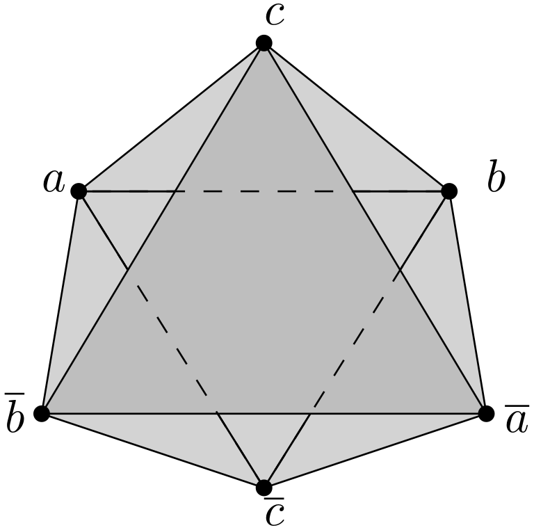
Figure 3. The polar complex for the example hypergraph in Figure 2.

Proposition 21.

The map $\Gamma:\mathrm{\textbf{Hyp}}\rightarrow\mathrm{\textbf{Simp}}$ is a functor.

Proof.

The object map is in Definition 19. Let $\mathcal{H}_{1},\mathcal{H}_{2}$ be two hypergraphs and $(f,g)$ be a morphism between them in Hyp (with $f:E_{1}\rightarrow E_{2}$ and $g:V_{1}\rightarrow V_{2}$). We define a map $\hat{g}:\Gamma(\mathcal{H}_{1})\rightarrow\Gamma(\mathcal{H}_{2})$ as follows:

$$\hat{g}(v)=\left\{\begin{tabular}[]{ll}$g(v)$&$v\in V$\\ $\overline{g(\overline{v})}$&v $\in\overline{V}$\end{tabular}\right..$$

In this definition note that $\overline{\overline{v}}:=v$. To make this concrete, if $g(x)=a$, then $\hat{g}(x)=a$ and $\hat{g}(\overline{x})=\overline{a}$. To complete the proof that $\Gamma$ is a functor we must show that $\hat{g}$ is a simplicial map.

Let $\sigma\in\Gamma(\mathcal{H}_{1})$ be a toplex. Then $\sigma$ corresponds to a hyperedge $e$ in $\mathcal{H}_{1}$ and we can write $\sigma=\epsilon_{1}(e)\sqcup\overline{V_{1}\setminus\epsilon_{1}(e)}$. Since $(f,g)$ is a morphism in Hyp the vertices in $e$ must be mapped to the vertices of $f(e)$. In particular, the vertices in $f(e)$ must form a hyperedge in $\mathcal{H}_{2}$. Therefore, there is a toplex in $\Gamma(\mathcal{H}_{2})$ equal to $\epsilon_{2}(f(e))\sqcup\overline{V_{2}\setminus\epsilon_{2}(f(e))}$. The vertices of the simplex $\sigma$ get mapped by $\hat{g}$ to $\{g(v):v\in\epsilon_{1}(e)\}\sqcup\{g(\overline{v}):v\in V_{1}\setminus\epsilon_{1}(e)\}$. The first half of this set is equal to $\epsilon_{2}(f(e))$ by the definition of a hypergraph morphism. The second half of the set may not be equal to $\overline{V_{2}\setminus\epsilon_{2}(f(e))}$ but it will be a subset. This is because it could be that $|V_{2}|>|V_{1}|$ and some vertices are not mapped to. Regardless, the image of $\sigma$ under $\hat{g}$ is a subset of a toplex in $\Gamma(\mathcal{H}_{2})$ and therefore it is a simplex in $\Gamma(\mathcal{H}_{2})$.

To show that a non-toplex $\tau\in\Gamma(\mathcal{H}_{1})$ maps to a simplex is then straightforward. $\tau$ must be a subset of a toplex $\sigma$. Since we just showed that a toplex maps to a simplex in $\Gamma(\mathcal{H}_{2})$, all of its subsets must map to subsets of that simplex.∎

3.5. Embedded homology

The idea of embedded homology, introduced by Bressan et al. [18], differs from the closure, barycentric, and polar complex homologies discussed previously in that it is not a simplicial complex that is constructed from the hypergraph but rather a chain complex. The construction starts with the chain complex from the upper closure and finds a particular sub-chain complex using only elements corresponding to the hyperedges such that the boundary maps are still valid. It is the chain complex homology (as described in Section 2.1.4) of this “infimum chain complex” that is called the embedded homology of the hypergraph. We give the formal details of this definition next.

Let ${\sf C}_{p}$ denote the $p$-dimensional chain group associated with $\Delta(\mathcal{H})$, as described in Section 3.1. That is, each element $c\in{\sf C}_{p}$ is a linear combination of the $p$-simplices in $\Delta(\mathcal{H})$ (with field coefficients). Together with boundary maps ${\mathrm{\partial}}_{p}:{\sf C}_{p}\to{\sf C}_{p-1}$, we have the following chain complex, denoted as ${\sf C}_{\bullet}$:

$$\cdots\to{\sf C}_{p}\xrightarrow{{\mathrm{\partial}}_{p}}{\sf C}_{p-1}\to\cdots.$$

Let $\mathsf{D}_{p}$ denote the collection of all linear combinations of $(p+1)$-hyperedges in $\mathcal{H}$ (with field coefficients). Then $\mathsf{D}_{p}$ is a subgroup of ${\sf C}_{p}$ for each $p$. The sequence of such subgroups is denoted $\mathsf{D}_{\bullet}$.

Given a chain complex ${\sf C}_{\bullet}$ and a sequence of subgroups $\mathsf{D}_{\bullet}$, the infimum chain group is defined as ${\mathsf{inf}}_{p}:={\mathsf{inf}}_{p}(\mathsf{D}_{p},{\sf C}_{p})=\mathsf{D}_{p}\cap{\mathrm{\partial}}^{-1}_{p}(\mathsf{D}_{p-1})$. We have the following commutative diagram:

where $j_{p}$ are chain maps induced by inclusions ${\mathsf{inf}}_{p}\to\mathsf{D}_{p}\to{\sf C}_{p}$, and $\delta_{p}={\mathrm{\partial}}_{p}\mid_{{\mathsf{inf}}_{p}}$, i.e., $\delta_{p}$ is the restriction of ${\mathrm{\partial}}_{p}$ to ${\mathsf{inf}}_{p}$. The chain map $j_{p}$ sends cycles to cycles, boundaries to boundaries, and thus induces a map on homology between $\mathsf{H}_{k}(\Delta(\mathcal{H})):=\mathsf{H}_{k}(C_{\bullet},{\mathrm{\partial}}_{\bullet})={\mathrm{ker\,}}{\mathrm{\partial}}_{k}/{\mathrm{im\,}}{\mathrm{\partial}}_{k+1}$ and $\mathsf{H}_{k}^{emb}(\mathcal{H}):=\mathsf{H}_{k}({\mathsf{inf}}_{\bullet},\delta_{\bullet})={\mathrm{ker\,}}\delta_{k}/{\mathrm{im\,}}\delta_{k+1}$. $\mathsf{H}_{k}^{emb}(\mathcal{H})$ is the $k$-th embedded homology of the hypergraph $\mathcal{H}$ as defined in [18].

We refer the reader to [18] for many theoretical results on embedded homology including a Mayer-Vietoris sequence and a persistence formulation. To serve these results they prove that embedded homology is a functor (although they do not use that word) from Hyp to Ab in their Proposition 3.7. The authors also provide some special cases of $\mathsf{H}_{\bullet}^{emb}$ when $\mathcal{H}$ is acyclic [14] and when $\mathcal{H}$ has one hyperedge that all other hyperedges are subsets of (i.e., if $\Delta(\mathcal{H})$ is a single simplex and all of its subsimplices). Bressan et al. also introduced some hypernetwork measures based on embedded homology for use in analyzing hypergraphs constructed from real-world data.

We return to our running example hypergraph from Figure 2 to show an example of embedded homology. To simplify, we use the notation $\langle X\rangle$ to be the group generated by the set $X$. In this example we have

${\sf C}_{2}=\langle abc\rangle$	$\mathsf{D}_{2}=\langle abc\rangle$	${\mathsf{inf}}_{2}(\mathsf{D}_{2},{\sf C}_{2})=\langle abc\rangle\cap{\mathrm{\partial}}_{2}^{-1}(\langle ab\rangle)=0$
${\sf C}_{1}=\langle ab,ac,bc\rangle$	$\mathsf{D}_{1}=\langle ab\rangle$	${\mathsf{inf}}_{1}(\mathsf{D}_{1},{\sf C}_{1})=\langle ab\rangle\cap{\mathrm{\partial}}_{1}^{-1}(\langle a,b,c\rangle)=\langle ab\rangle$
${\sf C}_{0}=\langle a,b,c\rangle$	$\mathsf{D}_{0}=\langle a,b,c\rangle$	${\mathsf{inf}}_{0}(\mathsf{D}_{0},{\sf C}_{0})=\langle a,b,c\rangle\cap{\mathrm{\partial}}_{0}^{-1}(0)=\langle a,b,c\rangle$

Given the infimum complex ${\mathsf{inf}}_{2}\xrightarrow{\delta_{2}}{\mathsf{inf}}_{1}\xrightarrow{\delta_{1}}{\mathsf{inf}}_{0}$, we see that $\mathsf{H}_{2}^{emb}(\mathcal{H})=\mathsf{H}_{1}^{emb}(\mathcal{H})=0$ and $\mathsf{H}_{0}^{emb}(\mathcal{H})=\mathbb{K}^{2}$ if homology is taken over the field $\mathbb{K}$.

Another illustrative example for the embedded homology is shown in Figure 4. Both hypergraphs have a cycle of edges, but for the hypergraph on the left it can be shown that $\beta_{1}^{emb}=1$ whereas on the right $\beta_{1}^{emb}=0$. This is because on the left the hypergraph cycle is made up of all edges of size 2 while on the right, one of the edges is of size 3. The preimage of $\mathsf{D}_{0}$ for the left hypergraph is all of $\mathsf{D}_{1}$ while on the right, it is just 0 since there is no cycle in the 1-dimensional edges. We can generalize this intuition by saying that embedded homology in dimension $p$ captures (among other things) uniform $p$-dimensional cycles even if not all (or even none!) of the sub-edges are present. This is in contrast to $\mathsf{H}_{\bullet}^{\Delta}$ which would have $\beta_{1}^{\Delta}=1$ in both of these examples because the simplex $\{a,b\}$ would be present as a sub-edge of $\{a,b,e\}$ in the hypergraph on the right.

(a) $\mathcal{H}_{1}$

(b) $\mathcal{H}_{2}$

Figure 4. Two hypergraphs to illustrate the fact that embedded homology captures “uniform cycles.”

Research in embedded homology is quite active. In particular, previous papers have explored computational aspects of embedded homology [73], developed relative embedded homology [88] and a persistence theory of hypergraph embedded homology [74], and explored applications in the context of biology [74], face-to-face interactions [74], and politics [99].

3.6. Hypergraph path homology

The path homology for hypergraphs was introduced by Grigor’yan et al. [50]. It builds upon path complexes and their homologies [49]. Recall a sequence in a finite nonempty set $X$ is a string of elements of $X$ in which repetitions are allowed and order matters.

Definition 22 ([49]).

For any nonnegative integer $p$, an elementary $p$-path over $X$ is a sequence of elements in $X$, $[x_{0},\dots,x_{p}]$, where $x_{0},\dots,x_{p}$ do not have to be distinct. Brackets are used in the notation for a $p$-path because the sequence will be playing the role of a simplex in a chain complex.

Let $\Lambda_{p}=\Lambda_{p}(X,{{\mathbb{K}}})$ denote the free vector space consisting of all formal linear combinations of elementary $p$-paths over $X$ with coefficients in a field ${{\mathbb{K}}}$. The elements of $\Lambda_{p}$ are called $p$-paths on $X$. Define $\Lambda_{-1}:={{\mathbb{K}}}$ and $\Lambda_{-2}:=\{0\}$. For any $p$, we define a boundary operator ${\mathrm{\partial}}:\Lambda_{p}\to\Lambda_{p-1}$ that is a linear operator acting on elementary paths,

(1) $${\mbox{$\mathrm{\partial}$}}([x_{0},\dots,x_{p}]):=\sum_{i=0}^{p}(-1)^{i}[x_{0},\dots,\hat{x}_{i},\dots,x_{p}].$$

Again, $\hat{x}_{i}$ means the omission of $x_{i}$. It can be shown that ${\mathrm{\partial}}^{2}=0$, and $\Lambda_{p}$ and ${\mathrm{\partial}}$ give rise to a standard chain complex, and an augmented chain complex, respectively:

$$\cdots\to\Lambda_{p}\to\Lambda_{p-1}\to\cdots\to\Lambda_{0}\to 0,$$

$$\cdots\to\Lambda_{p}\to\Lambda_{p-1}\to\cdots\to\Lambda_{0}\to{{\mathbb{K}}}\to 0.$$

The notion of a path complex arises from a finite nonempty set $X$. It generalizes the notions of a simplicial complex [50] and a digraph [49].

Definition 23.

[49, Definition 3.1] A path complex over a set $X$ is a nonempty collection $P:=P(X)$ of elementary paths on $X$ such that if $[x_{0},\dots,x_{p}]\in P$, then $[x_{1},\dots,x_{p}]\in P$ and $[x_{0},\dots,x_{p-1}]\in P$.

When a path complex $P$ is fixed, all the paths from $P$ are called allowed elementary paths. Definition 23 means that if we remove the first or the last element of an allowed $p$-path, then the resulting $(p-1)$-path is also allowed. Denote by $P_{p}$ the set of all $p$-paths from $P$. The set $P_{-1}$ contains a single empty path. Following [49], the elements of $P_{0}$ are called the vertices of $P$, and $P_{0}\subseteq X$. For simplicity, we will remove from the set $X$ all nonvertices so that $P_{0}=X$. A path complex contains elementary paths of varying lengths, $P=\{P_{p}\}_{p=0}^{\infty}$.

Given a path complex $P$ over a nonempty finite set $X$, we consider the linear space ${\mathcal{A}}_{p}:={\mathcal{A}}_{p}(P)$ that is spanned by all the elementary $p$-paths from $P$ (for any integer $p\geq-1$). The elements of ${\mathcal{A}}_{p}$ are called allowed $p$-paths. ${\mathcal{A}}_{p}$ is a subspace of $\Lambda_{p}$ by construction. We will restrict the operator ${\mathrm{\partial}}$ defined on spaces $\Lambda_{p}$ to the subspaces ${\mathcal{A}}_{p}$. In general, ${\mathrm{\partial}}{\mathcal{A}}_{p}$ does not have to be a subspace of ${\mathcal{A}}_{p-1}$. Therefore, we define a “well-behaved” subspace, $\Omega_{p}=\Omega_{p}(P)={\mathcal{A}}_{p}\cap{\mathrm{\partial}}^{-1}({\mathcal{A}}_{p-1})$. The elements of $\Omega_{p}$ are called ${\mathrm{\partial}}$-invariant (boundary invariant) $p$-paths. We thus obtain a standard chain complex of ${\mathrm{\partial}}$-invariant paths, and an augmented one, respectively:

$$\cdots\to\Omega_{p}\to\Omega_{p-1}\to\cdots\to\Omega_{0}\to 0,$$

$$\cdots\to\Omega_{p}\to\Omega_{p-1}\to\cdots\to\Omega_{0}\to{{\mathbb{K}}}\to 0.$$

The homology groups of the above chain complexes are referred to as the path homology and reduced path homology of the path complex $P$, denoted by $\mathsf{H}_{p}(P)$ ($p\geq 0$) and $\tilde{\mathsf{H}}_{p}(P)$ ($p\geq-1$) respectively, for $p\geq 0$ [49].

Definition 24 ([49]).

An elementary $p$-path $[x_{0},\dots,x_{p}]$ is a regular path if adjacent elements are distinct, that is, $x_{i}\neq x_{i+1}$ for $0\leq i\leq p-1$; otherwise it is an irregular path.

Regular paths are special types of elementary paths. Let ${\mathcal{R}}_{p}:={\mathcal{R}}_{p}(X,{{\mathbb{K}}})$ denote the span of the regular $p$-paths, i.e., the set of all finite linear combinations of regular $p$-paths. Let ${\mathcal{I}}_{p}:={\mathcal{I}}_{p}(X,{{\mathbb{K}}})$ denote the span of the irregular paths. It has been shown that ${\mathrm{\partial}}$ defined in (1) is not invariant on the family $\{{\mathcal{R}}_{p}\}$, but is invariant on $\{{\mathcal{I}}_{p}\}$. It has also been shown that ${\mathcal{R}}_{p}\cong\Lambda_{p}/{\mathcal{I}}_{p}$ via a natural linear isomorphism; we can define (with an abuse of notation) ${\mathrm{\partial}}:{\mathcal{R}}_{p}\to{\mathcal{R}}_{p-1}$ as the pull back of the boundary map ${\mathrm{\partial}}:\Lambda_{p}\to\Lambda_{p-1}$ via this isomorphism. This gives rise to another standard chain complex, together with an augmented one:

$$\cdots\to{\mathcal{R}}_{p}\to{\mathcal{R}}_{p-1}\to\cdots\to{\mathcal{R}}_{0}\to 0,$$

$$\cdots\to{\mathcal{R}}_{p}\to{\mathcal{R}}_{p-1}\to\cdots\to{\mathcal{R}}_{0}\to{{\mathbb{K}}}\to 0.$$

Homology groups of the above chain complexes are called the regular path homology and reduced regular path homology of $P$, denoted as $\mathsf{H}^{reg}_{p}(P)$ ($p\geq 0$) and $\tilde{\mathsf{H}}^{reg}_{p}(P)$ ($p\geq-1$), respectively.

Definition 25.

[49, Definition 3.4] A path complex $P$ is regular if all the paths $[x_{0},\dots,x_{p}]$ in $P$ are regular.

To define the path homology of a hypergraph $\mathcal{H}=(V,E)$, we define a path complex from $\mathcal{H}$ and study its homology.

Definition 26.

[50, Definition 5.5] For a hypergraph $\mathcal{H}=(V,E)$, define a path complex of density $q\geq 1$ on the set $V$ of vertices, denoted as $P^{q}(\mathcal{H})$, in the following way: a path of length $p\geq 0$ and density $q$ is defined as a sequence of $p+1$ vertices such that any $q$ consecutive vertices lie in some hyperedge of $\mathcal{H}$.

Definition 27.

[50] For a hypergraph $\mathcal{H}$ and any $q\geq 1$, we have a standard chain complex

$$\cdots\to\Omega_{p}(P^{q}(\mathcal{H}))\to\Omega_{p-1}(P^{q}(\mathcal{H}))\to\cdots\to\Omega_{0}(P^{q}(\mathcal{H}))\to 0.$$

The homology groups of the above chain complex are called the path homology of a hypergraph, denoted $\mathsf{H}_{p}(\mathcal{H},q)$. The regular path homology of a hypergraph, denoted $\mathsf{H}^{reg}_{p}(\mathcal{H},q)$, together with their reduced versions, are defined similarly.

We close this subsection with a proposition that the maximal edges determine the path homology of a hypergraph. This implies that path homology is constant on hyperblocks. The proof can be found in the cited paper.

Proposition 28.

[50, Proposition 5.6] The path homologies of a hypergraph, $\mathsf{H}_{p}(\mathcal{H},q)$ and $\mathsf{H}^{reg}_{p}(\mathcal{H},q)$, depend only on the set of its maximal edges.

3.7. Magnitude homology for hypergraphs

The Euler characteristic for finite categories [70] leads to a power series invariant of graphs called magnitude [71]. Hepworth and Willerton categorified magnitude of a graph, referred to as the magnitude homology [58] that inspired a geometric definition [6], Eulerian [47], blurred [81], and persistent magnitude homology [48], while raising questions about its structure [5, 53, 65, 91]. In particular, the original construction by Hepworth and Willerton [58] and the Eulerian magnitude homology by Giusti and Menara [47] are generalized from graphs to digraphs [59, 60], and to hypergraphs by Bi, Li, and Wu [17].

Magnitude homology of hypergraphs can be introduced in the light of path homology, see Section 3.6. The authors first generalized the notions of paths and distances between vertices of graphs to hypergraphs. This enables them to compute path length with values in $\mathbb{Z}[\frac{1}{2}].$ Instead of all sequences of vertices, it is sequences of hyperedges that generate magnitude chain groups for hypergraphs, analogous to the path homology of the dual hypergraph. The magnitude differential is the same as the path homology differential, obtained by removing a hyperedge from the sequence in all possible ways, with the additional condition that it only takes into account those paths obtained by removing a vertex from the sequence if it has the same length as the original path. This construction is functorial on hypergraphs and the authors also define simple magnitude for hypergraphs as an analogue of the regular path homology and a generalization of the Eulerian magnitude for graphs. To define the magnitude hypergraph homology, we follow [17].

Definition 29.

Let $e,f\in E$ denote hyperedges of a hypergraph $\mathcal{H}$. A path from $e$ to $f$ is a sequence of hyperedges $\gamma=e_{0}e_{1}\ldots e_{k}$ such that $e_{0}=e$, $e_{k}=f$, and every two consecutive hyperedges have a non-empty intersection. The height of such a path $h(\gamma)=k$ is one less than the number of hyperedges in the path and the length of the path $\gamma$ is $l(\gamma)=\sum_{i=0}^{k}l(e_{i},e_{i+1})$ where the length between two hyperedges is equal to

$$l(e,f)=\begin{cases}\infty&\text{if }e\cap f=\emptyset\\ 0&\text{if }e=f\\ \frac{1}{2}&\textrm{if }e\subsetneq f\text{ or }e\supsetneq f\\ 1&\text{otherwise.}\end{cases}$$

Definition 30.

Let $e,f\in E$ denote hyperedges of a hypergraph $\mathcal{H}.$ The intercrossing distance between $e$ and $f$ is defined by $d(e,f)=\inf_{\gamma}l(\gamma)$, where $\gamma$ denotes any path in $\mathcal{H}$ between $e$ and $f.$

Definition 31.

Given a hypergraph $\mathcal{H}$ and a sequence (tuple) $\gamma$ of hyperedges $\gamma=e_{0},e_{1},\ldots,e_{k}$, the length of $\gamma$ is defined as $\mathcal{L}(\gamma)=\sum_{i=0}^{k}d(e_{i},e_{i+1})$.

Note that the intercrossing distance endows the space of hypergraphs with the extended metric, so by the triangle inequality,

(2) $$\mathcal{L}(e_{0},e_{1},\ldots e_{i},\ldots,e_{k})\leq\mathcal{L}(e_{0},e_{1},\ldots\hat{e_{i}},\ldots,e_{k})$$

where $e_{0},e_{1},\ldots\hat{e_{i}},\ldots e_{k}$ denotes the sequence with the element $e_{i}$ removed.

Definition 32.

Given a hypergraph $\mathcal{H}$ and an abelian group ${\sf A}$, the magnitude chain complex ${\mathsf{MC}}(\mathcal{H};{\sf A})=\oplus_{l\geq 0}{\mathsf{MC}}_{\bullet,l}(\mathcal{H};{\sf A})$ where ${\mathsf{MC}}_{\bullet,l}(\mathcal{H};{\sf A})$ is a direct sum of groups ${\mathsf{MC}}_{k,l}(\mathcal{H};{\sf A})$ generated by sequences $e_{0},e_{1},\ldots e_{i},\ldots,e_{k}$ of length $l$ (implying that no two consecutive edges can be disjoint). The magnitude differential $\partial_{l}:{\mathsf{MC}}_{k,l}(\mathcal{H};{\sf A})\rightarrow{\mathsf{MC}}_{k-1,l}(\mathcal{H};{\sf A})$, $k\geq 0$ is defined as a sum $\partial_{l}=\sum_{i=0}^{k}(-1)^{i}\partial_{l,i}$ where $\partial_{l,i}:{\mathsf{MC}}_{k,l}(\mathcal{H};{\sf A})\rightarrow{\mathsf{MC}}_{k-1,l}(\mathcal{H};{\sf A})$ contains only tuples obtained by removing the element $e_{i}$ that remain length $l$:

$$\partial_{l,i}(e_{0},\ldots e_{i},\ldots,e_{k})=\begin{cases}e_{0},\ldots\hat{e_{i}},\ldots,e_{k}&\text{if }\mathcal{L}(e_{0},\ldots\hat{e_{i}},\ldots,e_{k})=l\\ 0&\text{otherwise.}\end{cases}$$

The magnitude hypergraph homology ${\mathsf{MH}}(\mathcal{H};{\sf A})$ of a hypergraph $\mathcal{H}$ with ${\sf A}$ coefficients is the homology of the magnitude hypergraph chain complex $({\mathsf{MC}}(\mathcal{H};{\sf A}),\partial).$

Unlike other homology theories in the current paper the magnitude hypergraph homology is bigraded with $k\in\mathbb{Z}$ and $l\in\mathbb{Z}[1/2]$ since lengths of tuples can be integers or multiples of $\frac{1}{2}$. Note that in [17] the authors compute the integral magnitude homology with ${\sf A}=\mathbb{Z}$, which determines magnitude homology with coefficients in a field such as $\mathbb{Z}_{2}.$ They additionally prove that ${\mathsf{MH}}_{0,0}(\mathcal{H};\mathbb{Z})=\mathbb{Z}^{\oplus|E|}$ and ${\mathsf{MH}}_{1,\frac{1}{2}}(\mathcal{H};\mathbb{Z})=\mathbb{Z}^{\oplus{|E|,2}}.$

Magnitude homology for graphs is related to path homology for graphs [4, 57], and it would be an interesting exploration to see if analogous relations existed on the level of hypergraphs.

3.8. Chromatic hypergraph homology

Categorification, first introduced and popularized in knot theory [67, 10], has inspired a number of categorifications in graph theory [25, 38, 55, 56, 92]. The idea behind categorifying a 1-variable polynomial with integer coefficients, such as the chromatic polynomial for graphs, can be lifted to a homology theory with an additional choice of algebra such as $A=\mathbb{Z}[x]/(x^{2}=0)$ [55]. Such a homology theory is bigraded with one grading corresponding to the number of edges and the other depending on the number of connected components of the graph/hypergraph labeled by the formal variable $x\in A$. A different categorification of the chromatic polynomial can be obtained by considering a manifold [38], and the two categorifications are related [11]. In the rest of this section, we introduce the chromatic hypergraph homology by Aslam and Sazdanovic [7, 8] which is related to the simplicial complex case [31]. The construction is illustrated in Figure 5.

Definition 33.

The state $s$ of a hypergraph $\mathcal{H}$ is a subset of hyperedges $s\subset E.$ An enhanced state on $\mathcal{H}$ denoted by $S=(s,\ell)$ consists of a state $s$ and an assignment $\ell$, where either $\ell=1$ or $\ell=x$, to each connected component $T_{k}$ of the partial hypergraph $[\mathcal{H}:s]$, which has the same vertex set as $\mathcal{H}$ but only edges in $s$.

Figure 5. The illustration of the chromatic hypergraph chain complex of a hypergraph G = (V = [3],{{a,b}, {b, c}}).

Next, for a labeled state $S$, let $i(S)$ be the number of hyperedges in the underlying state $s$ and $j(S)$ be the number of connected partial hypergraphs labeled by $x.$

Definition 34.

The chromatic hypergraph chain group $CC_{i,j}(\mathcal{H})$ for a hypergraph $\mathcal{H}$ is generated by all labeled states $S$ with $i(S)=i$ and $j(S)=j$. The $i$th chromatic chain group is the direct sum $CC_{i}(\mathcal{H}):=\bigoplus_{j\geq 0}CC_{i,j}(\mathcal{H})$ generated by all labelled states based on partial hypergraphs with exactly $i$ edges.

Figure 5 illustrates the chromatic hypergraph chain complex of a hypergraph $\mathcal{H}=(V=[3],\{\{a,b\},\{b,c\}\})$. $CC_{0}(\mathcal{H})$ is generated by labeled states based on the single state with just the vertices. Since there are 3 connected components we have $2^{3}=8$ labeling options since each component can be labeled by a $1$ or an $x$. Similarly, $CC_{1}(\mathcal{H})$ is the direct sum of two groups, one obtained by adding the blue edge $\{a,b\}$ and the other by adding the red $\{b,c\}.$ The two connected components, a vertex and an edge, can each be labeled by a $1$ or an $x$ for a total of four labeling options. Finally $CC_{2}(\mathcal{H})$ has a single state, namely the whole hypergraph $\mathcal{H}$ with a single connected component.

In order to define the chromatic differential $\partial^{C}_{i}:CC_{i,j}(\mathcal{H})\rightarrow CC_{i+1,j}(\mathcal{H})$, we need ordering on the hyperedges $f_{1},\ldots,f_{n}$ where $|E|=n$; however, the resulting chromatic hypergraph homology is independent of this choice [7, 8]. On the level of states, the differential is determined by adding a new hyperedge. On the level of the enhanced states the differential is determined by what effect adding a hyperedge has on the connected components of a given hypergraph.

For an enhanced state $S=(s,\ell)\in CC_{i,j}(\mathcal{H})$, we define the differential as

$$\partial^{C}_{i}(S):=\sum_{f\in E\setminus s}(-1)^{n(f)}S_{f},$$

where $n(f)$ is the number of hyperedges in $s$ that are lower in order than $f$. The labeling of the state $S_{f}=(s\cup f,\ell^{\prime})$ is obtained in the following way.

• if adding the hyperedge $f$ preserves the number of connected components then $S$ and $S_{f}$ have the same labels. This happens if the hyperedge $f$ being added is contained in one of the existing components.

• if adding the hyperedge $f$ connects components $T_{k_{1}}$ and $T_{k_{2}}$ of the state $s$, then $\ell^{\prime}(T_{k_{1}}\cup f\cup T_{k_{2}})=\ell(T_{k_{1}})\ell(T_{k_{2}})$ unless $\ell(T_{k_{1}})=\ell(T_{k_{2}})=x$, in which case $S_{f}=0$ is not a valid labeled state and does not contribute to the differential. In Figure 5, $\partial^{C}_{1}$ will be determined by multiplying labels of connected components with the following rules: the state labeled $(1,1)$ is mapped to $1$, $(1,x)$ or $(x,1)$ to $x$, but the state labeled $(x,x)$ is an element of the kernel.

All other labels in $\ell^{\prime}$ coincide with those from $l$.

Definition 35.

[7] The chromatic hypergraph homology ${\mathsf{CH}}(\mathcal{H})$ is the homology of the chain complex $(\displaystyle\bigoplus_{j\geq 0}CC_{i}(\mathcal{H}),\partial^{C})$ for $0\leq i\leq|E|.$

Since the chromatic hypergraph homology is a categorification of the chromatic polynomial, some of its properties lift those of the chromatic polynomial. The deletion-contraction formula lifts to a long exact sequence of homology groups [7].

It is important to say that chromatic homology is strictly better at distinguishing hypergraphs than the chromatic polynomial it categorifies. A pair of hypergraphs whose chromatic polynomials are identical but they are distinguished by their homology can be obtained by adding a hyperedge that contains all vertices of cochromatic graphs in [83, 87, 90]. We also note the following properties:

• If a hypergraph contains a hyperedge of size $1$, then its homology is trivial.

• Chromatic homology is preserved if all repeated hyperedges (edges with the same vertex set) are replaced by a single edge, and vice versa.

• Let $\theta_{n}$ denote the $n$-uniform hypergraph with a single hyperedge for $n>1$ that contains all vertices. Then with algebra $\mathcal{A}_{2}=\mathbb{Z}/(x^{2}=0)$ we have that homology is supported in degree zero: $CH_{0}(\theta_{n})=\mathbb{Z}^{n-1}\{1\}\oplus\bigoplus_{j=2}^{n}\mathbb{Z}^{\binom{n}{j}}\{j\}$. For example, for $\theta_{2}=\{[2],\{\{ab\}\}$ we have $\beta_{0}^{C}(\theta_{2})=2$ since $CH_{0,0}(\theta_{2})=\mathbb{Z}=CH_{0,1}$, and for $\theta_{3}=\{[3],\{\{abc\}\}$ the chromatic homology is $CH_{0,0}(\theta_{3})=\mathbb{Z}=CH_{0,3}$ and $CH_{0,2}(\theta_{3})=\mathbb{Z}^{\oplus 3}$ so $\beta_{0}^{C}(\theta_{3})=1+3+1=5.$

3.9. Weighted nerve and persistence

Thus far in this survey, we have presented hypergraph homology theories that consist of one computation of homology on a single topological object: a simplicial complex, chain complex, or relative chain complex. But a commonly used tool in topological data analysis is persistent homology (PH), which considers a filtration or a nested sequence of objects with inclusion maps from one to the next. If one computes homology of each of the objects in the sequence, the inclusion maps induce maps on the homology groups. This allows one to track the appearance and disappearance of topological features along indices of the filtration. We refer the reader to some standard introductions to persistent homology for details [23, 34, 39, 40, 44, 102].

The last hypergraph homology theory that we present is the persistent homology of a weighted simplicial complex. This structure is unique in that the hypergraph can be fully reconstructed from the weighted simplicial complex. We begin by defining the weighted nerve of a hypergraph.

Definition 36.

The weighted nerve complex, or simply weighted nerve, of a hypergraph $\mathcal{H}$, denoted ${\mathrm{Nrv}}_{w}(\mathcal{H})$, is the nerve of $\mathcal{H}$ (recall from Definition 2) weighted by $w(\sigma)=|\cap_{e\in\sigma}e|$.

An example weighted nerve for the hypergraph in Figure 2 is shown in Figure 6.

Figure 6. The weighted nerve (B) of the hypergraph $\mathcal{H}$ (A), also shown in Figure 2. Vertices are labeled by their weight followed by the name of the hyperedge they represent.

Before we define a filtration of the weighted nerve to compute persistence, we observe that if two hypergraphs have the same weighted nerve, they must be isomorphic.

Proposition 37.

If $\mathcal{H}_{1}$ and $\mathcal{H}_{2}$ are hypergraphs such that ${\mathrm{Nrv}}_{w}(\mathcal{H}_{1})={\mathrm{Nrv}}_{w}(\mathcal{H}_{2})$, then $\mathcal{H}_{1}\cong\mathcal{H}_{2}$.

The proof uses a Möbius inversion argument. In fact, the proof is constructive which implies that we can reconstruct the hypergraph from its weighted nerve up to relabeling of the vertices.

The Möbius inversion theorem states that given a weighted poset such that $w(x)=\sum_{y\leq x}f(y)$, the function $f$ is uniquely defined in terms of $w$ and the Möbius function on the poset. See [95, Sec. 3.7] for more details. In our setting, the poset is defined on ${\mathrm{Nrv}}(\mathcal{H})$ for a hypergraph $\mathcal{H}=(V,E)$ such that $\tau\leq\sigma$ iff $\tau\supseteq\sigma$. Note this means that $\cap_{e\in\tau}e\subseteq\cap_{e\in\sigma}e$. We first prove a helpful lemma and then return to the proof of Proposition 37.

Lemma 38.

Let $\mathcal{H}=(V,E)$ and ${\mathrm{Nrv}}_{w}(\mathcal{H})$ as defined above, then there is a unique function $f:{\mathrm{Nrv}}(\mathcal{H})\rightarrow\mathbb{R}$ such that $w(\sigma)=\sum_{\tau\leq\sigma}f(\tau)$.

Proof.

By Möbius inversion, if such an $f$ exists, then it must be unique. Therefore, it is enough to construct an $f$ that satisfies the desired equality. For every $v\in V$ let $\sigma(v):=\{e\in E:v\in e\}$, i.e., the set of all edges that $v$ is contained in. Note that $\sigma(v)\in{\mathrm{Nrv}}(\mathcal{H})$ because the intersection of the edges in this set must contain at least $v$. Define a function $f$ as follows:

$$f(\sigma):=\sum_{v\in\cap_{e\in\sigma}e}\mathbbm{1}_{\{\sigma(v)=\sigma\}}.$$

In words, $f(\sigma)$ is the number of vertices $v\in\cap_{e\in\sigma}e$ such that $v$ is in exactly the set of edges defined by $\sigma$ ($v$ is in no additional edges).

Consider the sum of $f$ over all simplices below $\sigma$:

$$\sum_{\tau\leq\sigma}f(\sigma) =\sum_{\tau\leq\sigma}\sum_{v\in\cap_{e\in\tau}e}\mathbbm{1}_{\{\sigma(v)=\tau\}}$$

$$=\sum_{\tau\leq\sigma}\left|\left\{v\in\bigcap_{e\in\tau}e:\sigma(v)=\tau\right\}\right|$$

$$=\left|\bigcup_{\tau\leq\sigma}\left\{v\in\bigcap_{e\in\tau}e:\sigma(v)=\tau\right\}\right|.$$

The final step in the above chain of equalities is true because the sets in the sum are disjoint for all $\tau$. Indeed, each $v$ has a unique $\sigma(v)$ and so is contained in only one such set. To show that $w(\sigma):=|\cap_{e\in\sigma}e|=\sum_{\tau\leq\sigma}f(\sigma)$ we need only show that

$$\bigcap_{e\in\sigma}e=\bigcup_{\tau\leq\sigma}\left\{v\in\bigcap_{e\in\tau}e:\sigma(v)=\tau\right\}.$$

$\subseteq$: Let $v\in\cap_{e\in\sigma}e$, then $\sigma(v)\leq\sigma$ so there exists a $\tau\leq\sigma$ such that $v\in\{v\in\cap_{e\in\tau}e:\sigma(v)=\tau\}$. Therefore $v\in RHS$.

$\supseteq$: Let $v\in\cup_{\tau\leq\sigma}\left\{v\in\cap_{e\in\tau}e:\sigma(v)=\tau\right\}$. Then there is a $\tau\leq\sigma$ such that $\sigma(v)=\tau$. Then $v\in\cap_{e\in\tau}e$. Since $\tau\leq\sigma$, $\sigma$ has fewer edges and so it must be that $v\in\cap_{e\in\sigma}e$ ∎

Now we are ready to prove Proposition 37.

Proof.

We have two hypergraphs, $\mathcal{H}_{1}$ and $\mathcal{H}_{2}$ such that ${\mathrm{Nrv}}_{w}(\mathcal{H}_{1})={\mathrm{Nrv}}_{w}(\mathcal{H}_{2})$. We can define an $f_{1}$ from $\mathcal{H}_{1}$ and an $f_{2}$ from $\mathcal{H}_{2}$ as in Lemma 38, so that

$$\sum_{\tau\leq\sigma}f_{1}(\tau)=w(\sigma)=\sum_{\tau\leq\sigma}f_{2}(\tau).$$

By Lemma 38 it must be that $f_{1}=f_{2}=:f$. So, what is left to show is that given such an $f$ on ${\mathrm{Nrv}}(\mathcal{H}_{1})={\mathrm{Nrv}}(\mathcal{H}_{2})$, there is a unique hypergraph (up to relabeling of vertices) that can give rise to it.

We know that $f(\sigma)$ is the number of vertices $v\in\cap_{e\in\sigma}e$ such that $v$ is in exactly the set of edges defined by $\sigma$. But we do not have to restrict ourselves to just $v\in\cap_{e\in\sigma}$; we could write $f(\sigma)$ as the number of vertices in $V$ that are in exactly the edges $e\in\sigma$. Since we have $f(\sigma)$ for every set $\sigma\subseteq E$ (any simplex $\tau\not\in{\mathrm{Nrv}}(\mathcal{H}_{i})$ has empty intersection and thus $f(\tau)=0$), and the vertex sets for any two $\sigma$ must be disjoint, there is a unique way (up to relabeling of vertices) to construct an incidence matrix, which in turn uniquely defines a hypergraph.

The number of vertices is equal to $n:=\sum_{\sigma\in Nrv(\mathcal{H}_{i})}f(\sigma)$ since every vertex has a unique $\sigma(v)$. WLOG we can label them as $V=\{v_{1},v_{2},\ldots,v_{n}\}$. The edges are the vertices in ${\mathrm{Nrv}}(\mathcal{H}_{1})={\mathrm{Nrv}}(H_{2})$. Also WLOG, order the simplices in ${\mathrm{Nrv}}(\mathcal{H}_{i})$, $\sigma_{0},\sigma_{1},\ldots,\sigma_{N}$. For each $\sigma_{j}$ let $s_{j}=\sum_{k<j}f(\sigma_{k})$ and assign vertices $v_{s_{j}+1},\ldots,v_{s_{j+1}}$ to all edges $e\in\sigma_{j}$. This assigns $s_{j+1}-(s_{j}+1)+1=s_{j+1}-s_{j}=f(\sigma_{j})$ unique vertices to all edges in $\sigma_{j}$ as required.

In summary, since $\mathcal{H}_{1}$ and $\mathcal{H}_{2}$ gave rise to the same weighted nerve they must have the same $f$ function which uniquely defines a hypergraph up to relabeling of vertices. Therefore $\mathcal{H}_{1}\cong\mathcal{H}_{2}$ as desired. ∎

This property of being able to recover the hypergraph from its weighted nerve is in contrast to all of the other constructions we explore in this survey. Indeed, every simplicial complex closure has many hypergraphs (i.e., everything in its hyperblock) that could give rise to it. The same is true for the restricted barycentric subdivision, relative barycentric subdivision, and polar complex, although homology is no longer constant across a hyperblock for these constructions. Likewise, it is also true for the chain complexes for embedded, path, magnitude, and chromatic homology. It is worth noting that a hypergraph cannot be reconstructed from its line graph, even one that is weighted by the number of vertices in each pairwise intersection. In fact, a hypergraph cannot be reconstructed from its weighted line graph together with the weighted line graph of its dual [68]. However, when one adds in all of the multi-way intersections weighted by their size, one has enough information to recover the hypergraph.

Our weighted nerve is closely related to structures introduced in [89] and [9], though what we do with them is different. In [89], Robinson introduces two weightings of the Dowker complex of a binary relation: the total weight and the differential weight. When a binary relation is interpreted as the incidence matrix of a hypergraph, the Dowker complex with total weight turns out to be the weighted nerve of the dual of the hypergraph. The differential weight is the same as the auxiliary weighting (the $f$ function) that we use in the proof. Robinson proves that the relation is recoverable from both weighted Dowker complexes through algorithmic proofs, but he does not make the Möbius connection between them. Baccini et al. [9] also study two weightings of the closure, though the weights that play the role of Robinson’s differential weights can be more general. This paper also comments that a reconstruction is possible.

While Robinson’s work proceeds by defining a cosheaf and Baccini et al. introduce a weighted Hodge Laplacian from the weighted simplicial complexes, we continue to our persistence filtration. It would be interesting future work to explore the connection between the cosheaf, the weighted Hodge Laplacian, and the persistent homology filtration of the weighted nerve. It follows directly from the definition of the weighted nerve that if $\sigma\subseteq\tau$, $\sigma$ corresponds to fewer hyperedges and thus $w(\sigma)\geq w(\tau)$. This allows us to construct a filtration of the weighted nerve and define the weighted nerve persistent homology of a hypergraph.

Definition 39.

Let $\mathcal{H}$ be a hypergraph and ${\mathrm{Nrv}}_{w}(\mathcal{H})$ be its weighted nerve. We create a filtration $X_{n}\subseteq X_{n-1}\subseteq\cdots\subseteq X_{0}$ where $X_{k}=\{\sigma\in{\mathrm{Nrv}}_{w}(\mathcal{H}):w(\sigma)\geq a_{k}\}$ (for some threshold $a_{k}$ that is monotonically decreasing). The persistent homology of this filtration is the weighted nerve persistent homology of hypergraph $\mathcal{H}$. A persistence barcode records the interval decomposition corresponding to the homology basis for each homological dimension $p$.

To continue the example in Figure 6, we get the following filtration:

$$\{F\}\subseteq\{D,F,DF\}\subseteq{\mathrm{Nrv}}_{w}(\mathcal{H}).$$

Applying persistent homology to this filtration, we get a single bar $[3,-\infty)$ in the $\mathsf{H}_{0}$ barcode and no other higher dimensional structure.

In prior sections, we proved that some of our simplicial complex constructions are functorial. In the case of the weighted nerve, we again cite [89] where Robinson proved that a cosheaf on the Dowker complex that is summarized by the weighted Dowker complex is functorial. While this seems to be promising for our weighted nerve, it is not clear that his result directly implies functoriality of the weighted nerve (or a cosheaf on the nerve), since the duality map is not a functor from Hyp to itself. However, since the hypergraph is fully recoverable from the weighted nerve, there may be a direct proof that does not require going through the duality map.

3.10. Other topological notions of hypergraphs

In this paper, we focus on simplicial, relative, and chain complex homology for hypergraphs. There are a variety of other methods in the literature to create topological structure from hypergraphs either from a topological or homological perspective. We briefly highlight a sampling of methods here for the interested reader to explore further.

Deepthi and Ramkumart create open sets from hyperedges to form a topological space, but they do not consider homology [33]. Diestel builds a homology theory for directed hypergraphs [35]. In [29], Chung and Graham consider cohomology rather than homology, with a particular focus on the space of all $\kappa$-uniform (i.e., every hyperedge has size $\kappa$) hypergraphs on a fixed vertex set rather than a single hypergraph. Emtander also restricts to $\kappa$-uniform hypergraphs as well as complete multi-partite hypergraphs, building simplicial complexes and computing Betti numbers from a Stanley-Reisner ring. The paper [80] also computes persistent homology on a hypergraph by instead constructing a metric from hypergraph data. The paper [72] also builds a persistence theory parametrized by a weight function by combining embedded homology with a notion of a neighborhood hypergraph model, and then applies this to discern the structure of molecules.

4. Building Intuition

Throughout Section 3, we provided a running example, computing all surveyed homology theories for the same hypergraph shown in Figure 2. This can build some level of intuition, but we provide even more examples in this section in an attempt to better understand the nuances of each homology theory. We do not claim to provide a complete characterization of any of these theories, but instead try to build intuition on questions like: which are the same for all hypergraphs in a hyperblock? If the homology is not constant on the hyperblock, how does adding sub-edges affect the homology? How does topological structure change by adding super-edges? Is there a relationship between the homology of a hypergraph and that of its dual? Future work could tackle these questions from a rigorous standpoint and prove which hypergraph modifications result in homology modifications for each theory.

In Table 1, we show the Betti numbers for several examples across multiple hyperblocks. In the following subsections, we make some remarks about the questions in the prior paragraph using examples from this table. We focus on fairly small hypergraphs so that computations can be completed. Row 2 corresponds to our running example in Figure 2. We use publicly available code in HyperNetX (HNX) [86] to compute the closure homology. We construct the polar complex from a hypergraph and then use HNX to compute its homology. For restricted and relative barycentric homology, we use an HNX module written by Christopher Potvin that implements computational efficiencies proved in his thesis [85]; this will be included in a future HNX release. We compute embedded homology and weighted nerve persistent homology by hand. Path homology is also computed by hand, but due to the combinatorial explosion of constructing paths, we only include a very small number of examples. The paper [17] shows detailed examples of the bi-graded magnitude homology, including the example in Row 7 of Table 1. As for chromatic homology, in Section 3.8, we provided some intuition on how hypergraph structure affects the homology. Since computation of chromatic homology by hand is more involved, we leave our intuition to those observations.

Row #	Hypergraph	$\beta_{\bullet}^{\Delta}$	$\beta_{\bullet}^{res}$	$\beta_{\bullet}^{rel}$	$\beta_{\bullet}^{pol}$	$\beta_{\bullet}^{emb}$	$\beta_{\bullet}^{path}$
1	$abc,ab,bc$	[1,0,0]	[1,0]	[0,1,0]	[1,0,0]	[0,0,0]	[1,0]
2	$abc,ab,a,b,c$	[1,0,0]	[1,0,0]	[0,1,0]	[1,2,0]	[2,0,0]	[1,0]
$2^{*}$	$ADF,BDF,CF$	[1,0,0]	[3,0,0]	[0,1,2]	[1,0,0,0,0]	[0,0,0]	X
3	$ab,bc$	[1,0]	[2,0]	[0,2]	[1,0,0]	[0,0]	[1,1]
4	$+a$	[1,0]	[2,0]	[0,1]	[1,0,0]	[1,0]	[1,1]
5	$+b$	[1,0]	[1,0]	[0,1]	[1,0,0]	[1,0]	[1,1]
6	$+a,c$	[1,0]	[2,0]	[0,0]	[1,1,0]	[1,0]	[1,1]
7	$+a,b$	[1,0]	[1,0]	[0,0]	[1,0,0]	[1,0]	[1,1]
8	$+a,b,c$	[1,0]	[1,0]	[1,0]	[1,1,0]	[1,0]	[1,1]
9	$abc,abd,acd,bcd$	[1,0,1]	[4]	[0,0,4]	[1,0,1,0]	[0,0,0]	X
10	$+a$	[1,0,1]	[2,0]	[0,0,2]	[1,0,1,0]	[1,0,0]	X
11	$+a,b$	[1,0,1]	[1,1]	[0,1,1]	[1,0,2,0]	[2,0,0]	X
12	$+a,b,c$	[1,0,1]	[1,3]	[0,3,1]	[1,0,4,0]	[3,0,0]	X
13	$+a,b,c,d$	[1,0,1]	[1,5]	[0,5,1]	[1,0,7,0]	[4,0,0]	X
14	$+ab$	[1,0,1]	[3,0]	[0,0,3]	[1,0,1,0]	[0,0,0]	X
15	$+ab,a,b$	[1,0,1]	[1,0,0]	[0,0,1]	[1,0,1,0]	[1,0,0]	X
16	$+ab,bc,a,b,c$	[1,0,1]	[1,1,0]	[0,1,1]	[1,0,2,0]	[1,0,0]	X
17	$+ab,bc,ac$	[1,0,1]	[1,0]	[0,0,1]	[1,0,1,0]	[0,0,0]	X
18	$+ab,bc,ac,a,b,c$	[1,0,1]	[1,0,0]	[0,0,1]	[1,0,1,0]	[0,0,0]	X
19	$abcde,abc,abd,acd,bcd$	[1,0,0,0,0]	[1,0]	[0,0,0,5,0]	[1,0,0,1,0]	[0,0,1,0,0]	X
20	$+ab,bc,ac$	[1,0,0,0,0]	[1,0,0]	[0,0,0,0,0]	[1,0,0,1,0]	[0,0,1,0,0]	X
21	$+abcd$	[1,0,0,0,0]	[1,0,0]	[0,0,0,0,0]	[1,0,0,0,0]	[0,0,0,0,0]	X
22	$abcde,bcdfg,abc,acd,abd$	[1,0,0,0,0]	[2,0]	[0,0,0,3,1]	[1,0,0,1,0,0,0]	[0,0,0,0,0]	X

Table 1. Table of Betti numbers for each homology theory across a variety of hypergraphs. The horizontal lines in the table break into distinct hyperblocks. The $+$ notation means we add the new hyperedge to the hypergraph in the first row of each hyperblock. For instance, in Row 14, we add hyperedge $\{ab\}$ to the four 3-edges (2-faces) of the tetrahedron in Row 9. Row 2* corresponds to the dual of the hypergraph in Row 2. In each cell, the vector is $[\beta_{0},\beta_{1},\cdots,\beta_{k}]$ for some value $k\leq dim(K)$, where $K$ is the auxiliary object we are taking homology of. The Xs in column $\beta_{\bullet}^{path}$ indicate the examples that we did not compute the path homology for.

4.1. Some initial intuition

We begin with the example in Row 19 of Table 1. This example illustrates a hypergraph which should “intuitively” have some homology in dimension 2. Consider the hypergraph that consists of the four 3-edges (2-faces) of the tetrahedron, together with a 5-edge containing all 4 vertices of the tetrahedron plus 1 additional vertex. One could consider this as a solid sphere (representing the 5-edge) with a tetrahedral void inside, which should have homology in dimension 2. Of course, the closure of this hypergraph is just the 4-dimensional simplex which has only $\beta_{0}^{\Delta}=1$ and no higher-dimensional homology. The relative barycentric homology of this example is also trivial as there is only one toplex. It is interesting that $\beta_{3}^{rel}=5$, so somehow quotienting by all of the missing sub-edges (of which there are many!) results in five 3-dimensional voids. But this is difficult to visualize. We also see in the table that $\beta_{3}^{pol}=1$. Embedded homology is the only homology theory, of the ones we computed, that aligns with the intuition that $\beta_{2}^{emb}=1$. We will come back to this example when we talk about adding sub-edges and super-edges.

A suggestion from Bubenik was to create a filtration of simplicial complexes, $\{K_{i}(\mathcal{H})\}$, where $K_{i}(\mathcal{H})=\Delta(\{e\in\mathcal{H}:|e|\leq i\})$. In this example, $K_{0}=\cdots=K_{2}=\emptyset$, $K_{3}=K_{4}=\Delta(\{abc,abd,acd,bcd\})$, and $K_{5}=\Delta(\mathcal{H})$. The persistent homology of this filtration has a bar $[3,5)$ in dimension 2 so this filtration “sees” the dimension 2 homology. However, if edge $bcdfg$ is added (along with new vertices $f$ and $g$), the tetrahedral void is both formed and killed at $K_{5}$ and so there is no bar in $\mathsf{H}_{2}$. This new edge replaces face $bcd$ with a larger edge and so whether this “should” have homology in dimension 2 is not clear. We show the Betti numbers for all other homology theories on Row 22 of the table and see that the feature that was in embedded homology in dimension 2 is no longer present. $\beta_{\bullet}^{pol}$ remains the same, as does $\beta_{\bullet}^{\Delta}$, but $\beta_{\bullet}^{res}$ and $\beta_{\bullet}^{rel}$ change.

4.2. Hyperblock variation

In Section 3.1, we observed that the closure homology is the same for all hypergraphs in a hyperblock since, by definition, all of these hypergraphs have the same closure. Similarly, in Section 3.6, we note that in [50] the authors prove hypergraph path homology depends only on the maximal hyperedges. Therefore, hypergraph path homology is constant on hyperblocks. However, it is clear from the table that $\mathsf{H}_{\bullet}^{res}$, $\mathsf{H}_{\bullet}^{rel}$, $\mathsf{H}_{\bullet}^{emb}$, and $\mathsf{H}_{\bullet}^{pol}$ are not constant on hyperblocks. In the next two subsections, we will make some observations about how adding sub- and super-edges can change the structure for these homology theories.

4.3. Adding sub-edges

When adding an edge, $e$, to a hypergraph, if there is already an edge $f$ such that $e\subseteq f$, we say that we are adding a sub-edge. This does not change the hyperblock but may change the homology for some of these homology theories. Here we describe some intuition gleaned from Table 1 about how adding sub-edges affects the structure.

Restricted barycentric homology

Recall from Proposition 15 that $\beta_{0}^{res}$ is maximized within a hyperblock by the simple hypergraph, the one with no sub-edges. If there are no sub-edges, then the edge containment poset is just the set of isolated vertices, one for each hyperedge, and so in addition to $\beta_{0}^{res}$ being maximized, $\beta_{k}^{res}=0$ for $k\geq 1$. As sub-edges are added, components can merge only if the added edge is a sub-edge of more than one edge. Structure can also be created in dimension 1 by adding sub-edges in a specific way. The canonical example is illustrated in moving from Row 9 to Row 11 in Table 1. Adding edges $a$ and $b$ to the hypergraph that already contains edges $abc$ and $abd$ creates a cycle between those four hyperedges in $\mathcal{O}(\mathcal{H})$, $a<abc>b<abd>a$, which translates to the cycle $\{a,abc,b,abd\}$. In the general case, whenever there is an intersection between two hyperedges, $e\cap f\neq\emptyset$, you can create a 1-dimensional cycle in $\mathcal{B}(\mathcal{H})$ by adding two non-comparable sub-edges, $g$ and $h$, within $e\cap f$. Continuing this operation of adding two non-comparable edges into the intersection $g\cap h$ will lift this 1-cycle into a 2-dimensional cycle. Adding these two edges effectively creates a suspension of the 1-cycle, creating an octahedron. Alternatively, we can destroy cycles by adding a sub-edge into the common intersection of all edges involved in the cycle, if an intersection exists. We thank Clara Buck for her insight into how adding sub-edges affects the restricted barycentric homology.

Relative barycentric homology

In Potvin’s thesis, he proved that if a hypergraph is simple then $\beta_{k-1}^{rel}(\mathcal{H})$ is equal to the number of hyperedges of size $k$. However, it’s not clear what adding sub-edges can do to the structure in general. We see in Rows 9-18 that adding subedges to the tetrahedron can change the homology significantly in $\beta_{\bullet}^{rel}$. This is true also for $\beta_{\bullet}^{res}$ but we understand more about how structure is formed and destroyed, as discussed above. It remains an open question to characterize how to create cycles in $\mathsf{H}_{\bullet}^{rel}$, even in dimension 1.

Polar complex homology

Little is known about the polar complex homology, but we observe in Table 1 that there is less variation in $\beta_{\bullet}^{pol}$ than in the other homology theories. We know that the total number of vertices in $\Gamma(\mathcal{H})$ is $2|V|$, each maximal simplex is of size $|V|$, and there are $|E|$ such maximal simplices. If a sub-edge, $f\subset e$, is added to the hypergraph then $\Sigma(e)\cap\Sigma(f)=f\cup\overline{(V\setminus e)}$. But how this changes the polar complex homology likely depends heavily on the structure of $\Gamma(\mathcal{H})$ and where the edge $f$ is added.

Embedded homology

In embedded homology, adding sub-edges helps to create structure, but it requires very specific sets of sub-edges. Given an edge $e$, if all of its sub-edges of size $|e|-1$ are present, then $e$ is present in $\inf_{|e|-1}$. But this is not the only way that $e$ can appear in $\inf_{|e|-1}$. For two edges $e,f$ with $|e|=|f|$, if all edges in ${\mathrm{\partial}}(e+f)$ are in the hypergraph, then $e+f$ is in $\inf_{|e|-1}$. Of course, making $\inf_{\bullet}$ larger does not necessarily create homological structure, but having $\inf_{\bullet}$ be nonzero is required for structure to be present. Therefore, understanding how sub-edges affect construction of the chain complex is a good first step. While embedded homology is well-studied and applied, we think there remain open questions that will help build intuition and characterize the relationship between structure in $\mathcal{H}$ and structure in $\mathsf{H}_{\bullet}^{emb}(\mathcal{H})$.

Weighted nerve persistent homology

As the weighted nerve persistent homology corresponds to an interval decomposition of features rather than a single homology computation, we display the barcode results in Table 2. From small examples (e.g., hypergraphs in Rows 1-2, 3-8, or 9-11 and 14), it might seem that adding sub-edges does not change the weighted nerve persistent homology. However, we note that the barcode for the hypergraph in Row 19, ${\mathsf{PH}}_{0}:\{[5,-\infty)\},{\mathsf{PH}}_{2}:\{[1,-\infty)\}$, is different from the weighted nerve persistent homology of the hypergraph $\{abcde\}$, which is in the same hyperblock. The barcode for $\{abcde\}$ is just $[5,-\infty)$ in dimension 0 as the weighted nerve is just a 0-simplex with weight 5. In fact, if you add sub-edges $\{abc,abd,acd\}$, the barcode of the weighted nerve persistent homology is still just $[5,-\infty)$ for ${\mathsf{PH}}_{0}$. But closing the inner tetrahedron creates some additional structure, which aligns with the intuition discussed in Section 4.1. In row 22 of Table 2 we see that the weighted nerve still captures nontrivial structure in dimension 2 when the second large edge is added. The weighted nerve is the only homology theory that captures dimension 2 structure in the row 22 example (while polar and relative barycentric homologies capture structure in dimension 3). We have not yet delved into studying the types of sub-edges that do or do not change the weighted nerve persistent homology but doing so would be an interesting question for future work.

Row #	Hypergraph	${\mathsf{PH}}_{0}$	${\mathsf{PH}}_{1}$	${\mathsf{PH}}_{2}$
1	$abc,ab,bc$	$\{[3,-\infty)\}$	$\emptyset$	$\emptyset$
2	$abc,ab,a,b,c$	$\{[3,-\infty)\}$	$\emptyset$	$\emptyset$
$2^{*}$	$ADF,BDF,CF$	$\{[3,-\infty),[3,2)\}$	$\emptyset$	$\emptyset$
3	$ab,bc$	$\{[2,-\infty),[2,1)\}$	$\emptyset$	$\emptyset$
4	$+a$	$\{[2,-\infty),[2,1)\}$	$\emptyset$	$\emptyset$
5	$+b$	$\{[2,-\infty),[2,1)\}$	$\emptyset$	$\emptyset$
6	$+a,c$	$\{[2,-\infty),[2,1)\}$	$\emptyset$	$\emptyset$
7	$+a,b$	$\{[2,-\infty),[2,1)\}$	$\emptyset$	$\emptyset$
8	$+a,b,c$	$\{[2,-\infty),[2,1)\}$	$\emptyset$	$\emptyset$
9	$abc,abd,acd,bcd$	$\{[3,-\infty),[3,2)\times 3)\}$	$\{[2,1)\times 3\}$	$\{[1,-\infty)\}$
10	$+a$	$\{[3,-\infty),[3,2)\times 3)\}$	$\{[2,1)\times 3\}$	$\{[1,-\infty)\}$
11	$+a,b$	$\{[3,-\infty),[3,2)\times 3)\}$	$\{[2,1)\times 3\}$	$\{[1,-\infty)\}$
14	$+ab$	$\{[3,-\infty),[3,2)\times 3)\}$	$\{[2,1)\times 3\}$	$\{[1,-\infty)\}$
19	$abcde,abc,abd,acd,bcd$	$\{[5,-\infty)\}$	$\emptyset$	$\{[1,-\infty)\}$
22	$abcde,bcdfg,abc,acd,abd$	$\{[5,-\infty),[5,3)\}$	$\emptyset$	$\{[1,-\infty)\}$

Table 2. Table of barcodes for weighted nerve persistence across a variety of hypergraphs sampled from examples in Table 1 (row numbering agrees).

4.4. Adding super-edges

While adding sub-edges cannot change the hyperblock of the hypergraph, there are two types of super-edges one could consider. In one case, you could add a super-edge that contains one or more toplexes; this would change the hyperblock of the hypergraph. Alternatively, you could add an edge $g$ that is a super-edge of a non-toplex and a sub-edge of a toplex; this would keep the hypergraph in the same hyperblock. We focus here on the former case rather than the latter.

We note that adding super-edges that contain one or more toplexes is somehow the reverse of adding sub-edges; therefore, much of what was said in the prior section has implications in this section. For example, in the case of restricted barycentric subdivision, if your hypergraph consists of two non-comparable hyperedges, $e$ and $f$, and you add two new hyperedges, $g$ and $h$, together with two new vertices, $x$ and $y$, such that $g=e\cup f\cup\{x\}$ and $h=e\cup f\cup\{y\}$, then you will create a 1-dimensional cycle in $\mathcal{B}(\mathcal{H})$. Of course, this is not the only way to add super-edges; in fact, it is quite specific and requires the addition of two super-edges. In general, adding a single edge has the effect of “coning off” any topological structure contained in the restricted barycentric subdivision of the set of edges it contains.

The example in the prior section for weighted nerve persistent homology is interesting in the case of adding super-edges as well. The barcode for the hollow tetrahedron hypergraph $\{abc,abd,acd,bcd\}$ (without singleton and pairwise edges, Row 9) is ${\mathsf{PH}}_{0}=\{[3,2)\times 3,[3,-\infty)\}$, ${\mathsf{PH}}_{1}=\{[2,1]\times 3\}$, and ${\mathsf{PH}}_{2}=\{[1,-\infty)\}$. When $\{abcde\}$ is added (Row 19), the simplex corresponding to this large edge connects to all of the sub-edges which pulls together the components that start at $k=3$. This super-edge also kills the dimension 1 features, but as noted above it does not kill the dimension 2 feature.

For the relative barycentric subdivision, Potvin again proved some helpful theorems. He introduces the notion of a maximum edge hypergraph which is one that contains an edge $e=V$. There may be many (or few) other hyperedges, but it at least has one containing all vertices. In this case, he proves that $\mathsf{H}_{n}^{rel}(\mathcal{H})\cong\mathsf{H}_{n-1}^{\Delta}(\mathcal{M}(\mathcal{H}))$ for $n\geq 2$, where we recall that $\mathcal{M}(\mathcal{H})$ is the missing subcomplex. This does not tell us how the structure changes with and without the maximum edge, but it does tell us how to compute the relative barycentric homology when a maximum edge is added.

Since adding super-edges of the toplexes will change the hyperblock, the path homology could also change; see the change from Row 3 to Row 1. Just as there was not much known about how adding sub-edges affects the polar complex and embedded homology, the same is true for adding super-edges. We encourage readers to consider studying these theories to help develop more understanding.

4.5. Duality

Duality is an operation that does not modify the hypergraph, but exchanges the roles of vertices and hyperedges. As we observed in Section 3.1, the closure homology of a hypergraph is isomorphic to the closure homology of its dual by Dowker duality. One might ask the question: is it true in general that the $X$-homology of a hypergraph is isomorphic to the $X$-homology of its dual (where $X$ is any of the homology theories introduced in this survey, or others developed in the future)? In fact, this is not generally true, and our running example in Figure 2 is a counterexample for $\mathsf{H}^{res},\mathsf{H}^{rel},\mathsf{H}^{pol}$, $\mathsf{H}^{emb}$, and for the persistent homology of the weighted nerve.

So, while it is generally not true that the $X$-homology of a hypergraph is isomorphic to the $X$-homology of its dual, one could instead ask the weaker question of whether or not there is any relationship between these two homologies. Perhaps there are some conditions on the hypergraph such that you can achieve an isomorphism. Or there could be a way to bound the difference between the $X$-homology of a hypergraph and the $X$-homology of its dual (perhaps with certain assumptions on hypergraph structure). This provides an interesting open question for future work. However, recall from Section 2.2.6 that duality is not a functor from Hyp to itself so one might expect that there would be no such relationship. Indeed it could be that for every $n>0$ you can find an $\mathcal{H}$ such that $|\beta_{k}^{\bullet}(\mathcal{H})-\beta_{k}^{\bullet}(\mathcal{H}^{*})|>n$.

For ${\mathsf{PH}}({\mathrm{Nrv}}_{w}(\mathcal{H}))$, we provide a pathological example to show that the number of bars in ${\mathsf{PH}}({\mathrm{Nrv}}_{w}(\mathcal{H}^{*}))$ can be arbitrarily more than the number of bars in ${\mathsf{PH}}({\mathrm{Nrv}}_{w}(\mathcal{H}))$. Consider our running example from Figure 2, but instead of the singleton edge with vertex $c$, we inflate that edge to contain $c_{1},\ldots,c_{n}$, as shown in Figure 7 along with its dual and their weighted nerves. Since the two nerves are homotopy equivalent (without weighting), the number of bars that continue to $-\infty$ must be the same. However, the barcode for ${\mathrm{Nrv}}_{w}(\mathcal{H})$ in dimension 0 consists of one bar $[n+2,-\infty)$ while the barcode for ${\mathrm{Nrv}}_{w}(\mathcal{H}^{*})$ in dimension 0 has bars $\{[3,-\infty),[3,2),[2,1)\times n\}$. Neither have persistent homology in dimension $k>0$. By duplicating a node arbitrarily many times (equivalently, duplicating an edge), we can make the two barcodes arbitrarily different in number of bars. This raises an open question of whether requiring the hypergraph to be collapsed allows us to bound or describe a relationship between the persistent homology of the weighted nerve of the hypergraph and that of its dual.

(a) $\mathcal{H}$

(b) $\mathcal{H}^{*}$

(c) ${\mathrm{Nrv}}_{w}(\mathcal{H})$

(d) ${\mathrm{Nrv}}_{w}(\mathcal{H}^{*})$

Figure 7. Pathological example for duality and the persistent homology of the weighted nerve.

5. Discussion

This survey provides detailed descriptions and known properties of nine homology theories for hypergraphs introduced and studied in recent years. We also include an intuition building section containing observations that come from computations on relatively small examples. The goal of this survey is to show that the research on homology theories for hypergraphs is active and to collect recent works in one place to observe similarities and differences among them. In doing so, we have identified some interesting open problems along the way; many are noted in the sections above. Beyond those identified above we leave readers with a few closing thoughts of where work in homology theories for hypergraphs could proceed.

Persistence and stability

In our survey, we include only one persistent homology theory for hypergraphs in Section 3.9. The weights on the closure are induced by the structure of the hypergraph. However, because of the functoriality results, many of the other theories can also be considered in a persistence context through the introduction of any kind of function on hyperedges or vertices. Consider, for example, the restricted barycentric homology. If we have a hypergraph $\mathcal{H}=(V,E)$ with a function on hyperedges $w:E\rightarrow\mathbb{R}$, we can induce a filtration $\mathcal{H}_{\alpha}=(V,E_{\alpha})$ where $E_{\alpha}=\{e\in E:w(e)\geq\alpha\}$. It is clear that $E_{\alpha}\subseteq E_{\beta}$ whenever $\alpha\leq\beta$ and so $\mathcal{H}_{\alpha}\rightarrow\mathcal{H}_{\beta}$ is a morphism in Hyp. By functoriality of $\mathsf{H}_{\bullet}^{res}$, $\{\mathcal{H}_{\alpha}\hookrightarrow\mathcal{H}_{\beta}\}$ induces a persistence module. This opens up many new questions like stability to perturbations of the function and interpretation of persistent homology for all these theories.

Characterizing structure through homology

One reason that a practitioner may want to study homology of a hypergraph is to get an understanding of some aspect of hypergraph structure that traditional hypernetwork sciences measures cannot quantify, for example to identify complex substructures. In [62], the authors propose that homology for hypergraphs, specifically for the restricted barycentric homology, can generalize graph motifs to hypergraphs in some way. The straightforward generalization of motifs from graphs to hypergraphs results in a combinatorial explosion (there are already nearly 2,000 hypergraph motifs with only 4 hyperedges [69]), but they argue that allowing small patterns to be unified if they have the same homological structure could be a way of combating that explosion. Understanding what kinds of small substructures are captured by each homology theory would be an interesting direction to pursue with potential application to hypergraph classification as in [77] for graphs.

Practical applications

Though it was noted that homology of hypergraphs could be useful for understanding structure of real world hypergraphs, there has been little work in that direction outside of the embedded homology work cited in Section 3.5 and [2]. A study in which each of these homology theories are computed and evaluated for hypergraphs coming from different application domains—e.g., biology, computer network data, collaborations—would be extremely valuable to the community. Achieving this requires developing additional computational tools, particularly for embedded, path, magnitude, and chromatic homology for hypergraphs. They also should be released as open source in order for the community to take advantage. We point to projects like HyperNetX and Open Applied Topology as potential packages where these tools could be incorporated.

References

- [1] Sinan G. Aksoy, Cliff Joslyn, Carlos Ortiz Marrero, Brenda Praggastis, and Emilie Purvine. Hypernetwork science via high-order hypergraph walks. EPJ Data Science, 9(1):1–34, December 2020.
- [2] Mehmet Emin Aktas, Thu Nguyen, Rakin Riza, Muhammad Ifte Islam, and Esra Akbas. Hypergraph classification via persistent homology. arXiv preprint arXiv:2306.11484, 2023.
- [3] Keri L. Anderson, Jeffrey S. Anderson, Sourabh Palande, and Bei Wang. Topological data analysis of functional MRI connectivity in time and space domains. In Connectomics in NeuroImaging: Second International Workshop, CNI 2018, Held in Conjunction with MICCAI 2018, Granada, Spain, September 20, 2018, Proceedings 2, pages 67–77. Springer, 2018.
- [4] Yasuhiko Asao. Magnitude homology and path homology. Bulletin of the London Mathematical Society, 55(1):375–398, 2023.
- [5] Yasuhiko Asao, Yasuaki Hiraoka, and Shu Kanazawa. Girth, magnitude homology and phase transition of diagonality. Proceedings of the Royal Society of Edinburgh Section A: Mathematics, 154(1):221–247, 2024.
- [6] Yasuhiko Asao and Kengo Izumihara. Geometric approach to graph magnitude homology. arXiv preprint arXiv:2003.08058, 2020.
- [7] Jai King Aslam. Categorifying the Chromatic Polynomial of a Hypergraph and TDA in Cancer Genomics. North Carolina State University, 2023.
- [8] Jai King Aslam and Radmila Sazdanovic. Chromatic hypergraph homology, polynomial, and coloring ideals. arXiv preprint arXiv:2203.11927, 2022.
- [9] Federica Baccini, Filippo Geraci, and Ginestra Bianconi. Weighted simplicial complexes and their representation power of higher-order network data and topology. Phys. Rev. E, 106:034319, Sep 2022.
- [10] Dror Bar-Natan. On Khovanov’s categorification of the jones polynomial. Algebraic & Geometric Topology, 2(1):337–370, 2002.
- [11] Vladimir Baranovsky and Radmila Sazdanovic. Graph homology and graph configuration spaces. Journal of Homotopy and Related Structures, 7(2):223–235, 2012.
- [12] Vladimir Batagelj and Andrej Mrvar. Some analyses of erdos collaboration graph. Social networks, 22(2):173–186, 2000.
- [13] Paul Bendich, James S. Marron, Ezra Miller, Alex Pieloch, and Sean Skwerer. Persistent homology analysis of brain artery trees. The annals of applied statistics, 10(1):198, 2016.
- [14] Claude Berge. Hypergraphs: combinatorics of finite sets, volume 45. Elsevier, 1984.
- [15] Dhananjay Bhaskar, William Y Zhang, Alexandria Volkening, Björn Sandstede, and Ian Y Wong. Topological data analysis of spatial patterning in heterogeneous cell populations: clustering and sorting with varying cell-cell adhesion. npj Systems Biology and Applications, 9(1):43, 2023.
- [16] Subhrajit Bhattacharya, Robert Ghrist, and Vijay Kumar. Persistent homology for path planning in uncertain environments. IEEE Transactions on Robotics, 31(3):578–590, 2015.
- [17] Wanying Bi, Jingyan Li, and Jie Wu. The magnitude homology of a hypergraph. to appear: Homology, Homotopy and Applications, 2023.
- [18] Stephane Bressan, Jingyan Li, Shiquan Ren, and Jie Wu. The embedded homology of hypergraphs and applications. Asian Journal of Mathematics, 23(3):479–500, June 2019. Publisher: International Press of Boston.
- [19] Alain Bretto. Hypergraph theory. An introduction. Mathematical Engineering. Cham: Springer, 1, 2013.
- [20] Rickard Brüel-Gabrielsson, Vignesh Ganapathi-Subramanian, Primoz Skraba, and Leonidas J. Guibas. Topology-aware surface reconstruction for point clouds. Computer Graphics Forum, 39(5):197–207, 2020.
- [21] Gunnar Carlsson and Vin De Silva. Zigzag persistence. Foundations of computational mathematics, 10(4):367–405, 2010.
- [22] Gunnar Carlsson and Mikael Vejdemo-Johansson. Topological Data Analysis with Applications. Cambridge University Press, 2021.
- [23] Gunnar E. Carlsson. Topology and data. Bulletin of the American Mathematical Society, 46:255–308, 2009.
- [24] Henry Cartan and Samuel Eilenberg. Homological Algebra (PMS-19), Volume 19. Princeton university press, 2016.
- [25] Alex Chandler, Radmila Sazdanovic, Salvatore Stella, and Martha Yip. On the strength of chromatic symmetric homology for graphs. Advances in Applied Mathematics, 150:102559, 2023.
- [26] Samir Chowdhury and Facundo Mémoli. A functorial dowker theorem and persistent homology of asymmetric networks. Journal of Applied and Computational Topology, 2(1):115–175, 2018.
- [27] Samir Chowdhury and Facundo Mémoli. Persistent Path Homology of Directed Networks. In Proceedings of the 2018 Annual ACM-SIAM Symposium on Discrete Algorithms (SODA), Proceedings, pages 1152–1169. Society for Industrial and Applied Mathematics, January 2018.
- [28] Samir Chowdhury, Tom Needham, Ethan Semrad, Bei Wang, and Youjia Zhou. Hypergraph Co-Optimal transport: Metric and categorical properties. Journal of Applied and Computational Topology (APCT), 2023.
- [29] F.R.K. Chung and R.L. Graham. Cohomological aspects of hypergraphs. Transactions of the American Mathematical Society, 334(1):365–388, 1992.
- [30] Moo K Chung, Alexander Smith, and Gary Shiu. Reviews: Topological distances and losses for brain networks. arXiv preprint arXiv:2102.08623, 2021.
- [31] Andrew A. Cooper, Vin de Silva, and Radmila Sazdanović. On configuration spaces and simplicial complexes. New York J. Math, 25:723–744, 2019.
- [32] Harold Scott Macdonald Coxeter. Regular polytopes. Courier Corporation, 1973.
- [33] Chandran R. Deepthi and P.B. Ramkumar. Hypergraph topology. In Topological Dynamics and Topological Data Analysis: IWCTA 2018, Kochi, India, December 9–11, pages 271–278. Springer, 2021.
- [34] Tamal K. Dey and Yusu Wang. Computational Topology for Data Analysis. Computational Topology for Data Analysis. Cambridge University Press, 2022.
- [35] Reinhard Diestel. Homological aspects of oriented hypergraphs. arXiv preprint arXiv:2007.09125, 2020.
- [36] Willibald Dörfler and D.A. Waller. A category-theoretical approach to hypergraphs. Archiv der Mathematik, 34:185–192, 1980.
- [37] Clifford H. Dowker. Homology groups of relations. Annals of mathematics, pages 84–95, 1952.
- [38] Michael Eastwood and Stephen Huggett. Euler characteristics and chromatic polynomials. European Journal of Combinatorics, 28(6):1553–1560, 2007.
- [39] Herbert Edelsbrunner and John Harer. Computational topology: an introduction. American Mathematical Soc., 2010.
- [40] Herbert Edelsbrunner, David Letscher, and Afra Zomorodian. Topological persistence and simplification. Discrete & Computational Geometry, 28:511–533, 2002.
- [41] Ronald Fagin. Degrees of acyclicity for hypergraphs and relational database schemes. Journal of the ACM (JACM), 30(3):514–550, 1983.
- [42] Michelle Feng and Mason A. Porter. Persistent homology of geospatial data: A case study with voting. SIAM Review, 63(1):67–99, 2021.
- [43] Ellen Gasparovic, Maria Gommel, Emilie Purvine, Radmila Sazdanovic, Bei Wang, Yusu Wang, and Lori Ziegelmeier. A complete characterization of the one-dimensional intrinsic čech persistence diagrams for metric graphs. In Research in Computational Topology, pages 33–56. Springer, 2018.
- [44] Robert W. Ghrist. Elementary applied topology, volume 1. Createspace Seattle, WA, 2014.
- [45] Barbara Giunti, Jānis Lazovskis, and Bastian Rieck. DONUT: Database of Original & Non-Theoretical Uses of Topology, 2022. https://donut.topology.rocks.
- [46] Chad Giusti, Robert Ghrist, and Danielle S. Bassett. Two’s company, three (or more) is a simplex. Journal of computational neuroscience, 41(1):1–14, 2016.
- [47] Chad Giusti and Giuliamaria Menara. Eulerian magnitude homology: subgraph structure and random graphs. arXiv preprint arXiv:2403.09248, 2024.
- [48] Dejan Govc and Richard Hepworth. Persistent magnitude. Journal of Pure and Applied Algebra, 225(3):106517, 2021.
- [49] A. A. Grigor’yan, Yong Lin, Yu. V. Muranov, and Shing-Tung Yau. Path Complexes and their Homologies. Journal of Mathematical Sciences, 248(5):564–599, August 2020.
- [50] Alexander Grigor’yan, Rolando Jimenez, Yuri Muranov, and Shing-Tung Yau. Homology of path complexes and hypergraphs. Topology and its Applications, 267:106877, 2019.
- [51] Will Grilliette. Simplification & incidence: How an incidence-focused perspective patches category-theoretic problems in graph theory. arXiv preprint arXiv:2403.13165, 2024.
- [52] Will Grilliette and Lucas J Rusnak. Incidence hypergraphs: The categorical inconsistency of set-systems and a characterization of quiver exponentials. arXiv preprint arXiv:1805.07670, 2018.
- [53] Yuzhou Gu. Graph magnitude homology via algebraic morse theory. arXiv preprint arXiv:1809.07240, 2018.
- [54] Allen Hatcher. Algebraic topology. Cambridge Univ. Press, Cambridge, 2000.
- [55] L. Helme-Guizon and Y. Rong. A categorification for the chromatic polynomial. Algebraic & Geometric Topology, 5(4):1365–1388, 2005.
- [56] Laure Helme-Guizon and Yongwu Rong. Graph cohomologies from arbitrary algebras. arXiv preprint math/0506023, 2005.
- [57] Richard Hepworth and Emily Roff. Bigraded path homology and the magnitude-path spectral sequence. arXiv preprint arXiv:2404.06689, 2024.
- [58] Richard Hepworth and Simon Willerton. Categorifying the magnitude of a graph. Homology, Homotopy and Applications, 19(2):31–60, 2017.
- [59] Steve Huntsman. Magnitude and topological entropy of digraphs. arXiv preprint arXiv:2205.05178, 2022.
- [60] Steve Huntsman. Magnitude of arithmetic scalar and matrix categories. arXiv preprint arXiv:2304.08334, 2023.
- [61] Vladimir Itskov, Alexander Kunin, and Zvi Rosen. Hyperplane neural codes and the polar complex. In Topological Data Analysis: The Abel Symposium 2018, pages 343–369. Springer, 2020.
- [62] Helen Jenne, Sinan G. Aksoy, Daniel Best, Alyson Bittner, Gregory Henselman-Petrusek, Cliff Joslyn, Bill Kay, Audun Myers, Garret Seppala, Jackson Warley, et al. Stepping out of flatland: Discovering behavior patterns as topological structures in cyber hypergraphs. The Next Wave, 25(1), 2024.
- [63] Cliff A. Joslyn, Sinan G. Aksoy, Tiffany J Callahan, Lawrence E Hunter, Brett Jefferson, Brenda Praggastis, Emilie Purvine, and Ignacio J Tripodi. Hypernetwork science: from multidimensional networks to computational topology. In International conference on complex systems, pages 377–392. Springer, 2020.
- [64] Jonas L. Juul, Austin R. Benson, and Jon Kleinberg. Hypergraph patterns and collaboration structure. Frontiers in Physics, 11:1301994, 2024.
- [65] Ryuki Kaneta and Masahiko Yoshinaga. Magnitude homology of metric spaces and order complexes. ArXiv e-prints, 2018.
- [66] Firas A. Khasawneh, Elizabeth Munch, and Jose A. Perea. Chatter classification in turning using machine learning and topological data analysis. IFAC-PapersOnLine, 51(14):195–200, 2018. 14th IFAC Workshop on Time Delay Systems TDS 2018.
- [67] Mikhail Khovanov. A categorification of the jones polynomial. arXiv preprint math/9908171, 1999.
- [68] Steve Kirkland. Two-mode networks exhibiting data loss. Journal of Complex Networks, 6(2):297–316, 2018.
- [69] Geon Lee, Jihoon Ko, and Kijung Shin. Hypergraph motifs: concepts, algorithms, and discoveries. Proceedings of the VLDB Endowment, 13(12):2256–2269, 2020.
- [70] Tom Leinster. The Euler characteristic of a category. Documenta Mathematica, 13:21–49, 2008.
- [71] Tom Leinster. The magnitude of a graph. Mathematical Proceedings of the Cambridge Philosophical Society, 166(2):247–264, 2019.
- [72] Jian Liu, Dong Chen, Jingyan Li, and Jie Wu. Neighborhood hypergraph model for topological data analysis. Computational and Mathematical Biophysics, 10(1):262–280, 2022.
- [73] Xiang Liu, Huitao Feng, Jie Wu, and Kelin Xia. Computing hypergraph homology. Foundations of Data Science, 6(2):172–194, 2024.
- [74] Xiang Liu, Xiangjun Wang, Jie Wu, and Kelin Xia. Hypergraph-based persistent cohomology (HPC) for molecular representations in drug design. Briefings in Bioinformatics, 22(5):bbaa411, 01 2021.
- [75] Saunders Mac Lane. Categories for the working mathematician, volume 5. Springer Science & Business Media, 2013.
- [76] Melissa R. McGuirl, Alexandria Volkening, and Björn Sandstede. Topological data analysis of zebrafish patterns. Proceedings of the National Academy of Sciences, 117(10):5113–5124, 2020.
- [77] Ron Milo, Shai Shen-Orr, Shalev Itzkovitz, Nadav Kashtan, Dmitri Chklovskii, and Uri Alon. Network motifs: simple building blocks of complex networks. Science, 298(5594):824–827, 2002.
- [78] Mark E.J. Newman. The structure of scientific collaboration networks. Proceedings of the national academy of sciences, 98(2):404–409, 2001.
- [79] Mark E.J. Newman. Who is the best connected scientist? a study of scientific coauthorship networks. In Complex networks, pages 337–370. Springer, 2004.
- [80] Dong Quan Ngoc Nguyen, Lin Xing, and Lizhen Lin. Community detection, pattern recognition, and hypergraph-based learning: approaches using metric geometry and persistent homology. In Fuzzy Systems and Data Mining VI, pages 457–473. IOS Press, 2020.
- [81] Nina Otter. Magnitude meets persistence. homology theories for filtered simplicial sets. arXiv preprint arXiv:1807.01540, 2018.
- [82] Nina Otter, Mason A. Porter, Ulrike Tillmann, Peter Grindrod, and Heather A. Harrington. A roadmap for the computation of persistent homology. EPJ Data Science, 6:1–38, 2017.
- [83] Milena D Pabiniak, Józef H Przytycki, and Radmila Sazdanović. On the first group of the chromatic cohomology of graphs. Geometriae Dedicata, 140(1):19, 2009.
- [84] AD Parks and SL Lipscomb. Homology and hypergraph acyclicity: A combinatorial invariant for hypergraphs. https://apps.dtic.mil/sti/pdfs/ADA241584.pdf, 1991.
- [85] Christopher Potvin. Hypergraphs and Their Homology. PhD thesis, Michigan State University, 2023.
- [86] Brenda Praggastis, Sinan Aksoy, Dustin Arendt, Mark Bonicillo, Cliff Joslyn, Emilie Purvine, Madelyn Shapiro, and Ji Young Yun. Hypernetx: A python package for modeling complex network data as hypergraphs. Journal of Open Source Software, 9(95):6016, 2024.
- [87] Józef H Przytycki and Radmila Sazdanovic. Torsion in khovanov homology of semi-adequate links. arXiv preprint arXiv:1210.5254, 2012.
- [88] Shiquan Ren, Jie Wu, and Mengmeng Zhang. The embedded homology of hypergraph pairs. Journal of Knot Theory and Its Ramifications, 31(14):2250103, 2022.
- [89] Michael Robinson. Cosheaf representations of relations and dowker complexes. Journal of Applied and Computational Topology, 6(1):27–63, 2022.
- [90] Radmila Sazdanovic and Daniel Scofield. Patterns in khovanov link and chromatic graph homology. Journal of Knot Theory and Its Ramifications, 27(03):1840007, 2018.
- [91] Radmila Sazdanovic and Victor Summers. Torsion in the magnitude homology of graphs. Journal of Homotopy and Related Structures, 16(2):275–296, 2021.
- [92] Radmila Sazdanovic and Martha Yip. A categorification of the chromatic symmetric function. Journal of Combinatorial Theory, Series A, 154:218–246, 2018.
- [93] Ankit Sharma. Hypergraph Analytics: Modeling Higher-order Structures and Probabilities. PhD thesis, University of Minnesota, 2020.
- [94] Gurjeet Singh, Facundo Mémoli, and Gunnar E Carlsson. Topological methods for the analysis of high dimensional data sets and 3d object recognition. SPBG, 91:100, 2007.
- [95] Richard P Stanley. Enumerative Combinatorics, Volume 1. Cambridge University Press, 1997.
- [96] Ulrich Stelzl, Uwe Worm, Maciej Lalowski, Christian Haenig, Felix H. Brembeck, Heike Goehler, Martin Stroedicke, Martina Zenkner, Anke Schoenherr, Susanne Koeppen, et al. A human protein-protein interaction network: a resource for annotating the proteome. Cell, 122(6):957–968, 2005.
- [97] Chad M. Topaz, Lori Ziegelmeier, and Tom Halverson. Topological data analysis of biological aggregation models. PloS one, 10(5), 2015.
- [98] Pietro Traversa, Guilherme Ferraz de Arruda, Alexei Vazquez, and Yamir Moreno. Robustness and complexity of directed and weighted metabolic hypergraphs. Entropy, 25(11):1537, 2023.
- [99] Ismar Volic and Zixu Wang. Hypergraphs and political structures. arXiv preprint arXiv:2404.14638, 2024.
- [100] Pengxiang Wu, Chao Chen, Yusu Wang, Shaoting Zhang, Changhe Yuan, Zhen Qian, Dimitris Metaxas, and Leon Axel. Optimal topological cycles and their application in cardiac trabeculae restoration. In Information Processing in Medical Imaging: 25th International Conference, IPMI 2017, Boone, NC, USA, June 25-30, 2017, Proceedings 25, pages 80–92. Springer, 2017.
- [101] Lin Yan, Talha Bin Masood, Raghavendra Sridharamurthy, Farhan Rasheed, Vijay Natarajan, Ingrid Hotz, and Bei Wang. Scalar field comparison with topological descriptors: Properties and applications for scientific visualization. Computer Graphics Forum, 40(3):599–633, 2021.
- [102] Afra Zomorodian and Gunnar Carlsson. Computing persistent homology. Discrete & Computational Geometry, 33(2):249–274, 2005.