Reexamination of vacuum-polarization corrections
to the self-energy in muonic bound systems

Abstract

In muonic bound systems, the dominant radiative correction is due to vacuum polarization. Yet, for the interpretation of precision experiments, self-energy effects are also important. In turn, additional vacuum-polarization loops perturb the self-energy. Here, we show that combined self-energy vacuum-polarization effects can perturb the bound-state self-energy at the percent level in one-muon bound systems with nuclear charges $Z=1$—$6$. We also update previous treatments of the corrections for muonic hydrogen, muonic deuterium, and muonic helium bound systems.

I Introduction

The one-loop electronic vacuum-polarization (eVP) correction to the Coulomb potential constitutes the most numerically important radiative correction for the energies of bound states in muonic bound systems. Due to the smaller effective Bohr radius as compared to electronic systems, the muon penetrates the vacuum-polarized charge cloud around the nucleus very effectively, and the bound muon is exposed to a mean electric field strength, which, even for nuclear charge numbers $Z>3$, surpasses not only the field strength achievable in highly charged hydrogenlike ions with the heaviest nuclei, but also, Schwinger’s critical electric field strength (see Fig. 3 of Ref. Je2015muonic ).

Specifically, the leading energy shift mediated by eVP in muonic bound systems is of the order of $\alpha(Z\alpha)^{2}m_{r}$, where $m_{r}$ is the reduced mass of the bound system, $Z$ is the nuclear charge, and $\alpha$ is the fine-structure constant (we set $\hbar=c=\epsilon_{0}=1$). Self-energy (SE) shifts, by contrast, are parametrically suppressed in muonic bound systems, and are of order $\alpha(Z\alpha)^{4}m_{r}$, enhanced by a logarithm of $Z\alpha$. Except for the logarithmic enhancement, this is the same magnitude as the correction due to vacuum polarization with muon loops ($\mu$VP), as well as the first-order relativistic correction to the eVP (see Ref. Pa1996muonic ).

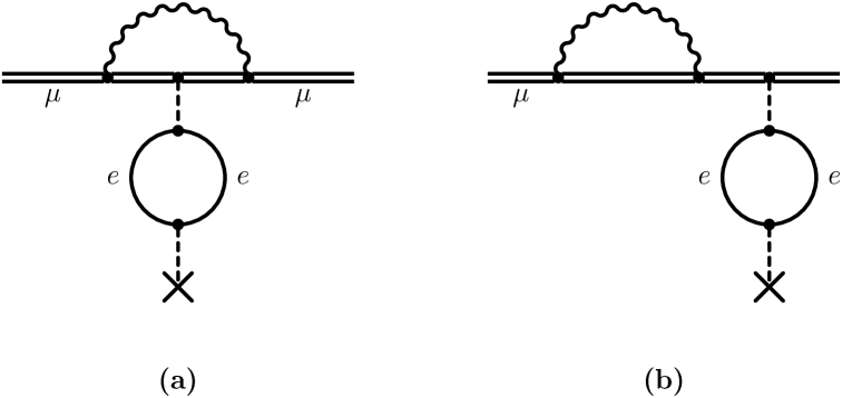
Figure 1: The Feynman diagrams for the vacuum-polarization correction to the self-energy comprise a vacuum-polarization insertion (a) into a Coulomb photon of the vertex diagram and the second-order effect (b).

In electronic systems, the next-to-leading correction to the SE is of order $\alpha(Z\alpha)^{5}m_{r}$; it was calculated by Baranger, Bethe, and Feynman BaBeFe1953 (see also Chap. 15 of Ref. JeAd2022book ). In muonic systems, by contrast, the eVP-mediated binding correction to the SE (SE-eVP), of which the corresponding diagrams are shown in Fig. 1, is logarithmically enhanced and of order $\alpha^{2}(Z\alpha)^{4}\,\ln[(Z\alpha)^{-2}]m_{r}$; it is thus of comparable magnitude to the effect of order $\alpha(Z\alpha)^{5}m_{r}$, if not larger. In light muonic atoms, this effect is the largest out of all corrections which enter at $\alpha^{2}(Z\alpha)^{4}m_{r}$ KaIvKa2013 , as illustrated in Fig. 2.

Figure 2: Magnitude of various contributions to the $2P_{1/2}$–$2S$ Lamb shift in light muonic atoms, in units of $(\frac{\alpha}{\pi})^{2}\frac{(Z\alpha)^{4}}{8}\frac{m_{r}^{3}}{m_{\mu}^{2}}$. Contributions specific to muonic atoms are denoted with circles and include the self-energy with electronic vacuum polarization (SE-eVP) calculated in this work. The eVP insertion into the radiative photon of the one-loop self energy is denoted as SE(eVP); it is taken from Eqs. (65)—(68) from Ref. PaEtAl2024 . The relativistic contributions to two-loop eVP (Rel. eVP2, without recoil corrections to that effect) are taken from Tables II and IV of Ref. KaIvKa2013 , and Tables I—III of Ref. KrMaMaSu2016 . The one-loop eVP with one-loop $\mu$VP (eVP-$\mu$VP) is taken from Table VIII of Ref. KaIvKa2013 and Tables I-III of Ref. KrMaMaSu2016 . From Table 3 in YePaPa2019 , we can scale contributions originally obtained for electronic systems, namely, the two-loop self-energy SE2, the two-loop muonic vacuum polarization $\mu$VP2, and the combination of self-energy and muonic vacuum polarization SE-$\mu$VP. These scaled contributions are denoted with squares.

The SE-eVP effect in muonic atoms was first considered by Pachucki, who calculated it in the leading logarithmic approximation [Eq. (39) in Pa1996muonic ]. The numerical result for the $2P$–$2S$ Lamb shift in muonic hydrogen was $-0.5~{}\mu$eV. Eides et al.. included it in their compilation, with an estimated uncertainty of $20\%$ EiGrSh2001 . However, calculations beyond the leading-log approximation have shown that there is a strong cancelation between the leading logarithmic effect and the vacuum-polarization correction to the nonlogarithmic term WuJe2011 , so that the approximation only gives the correct order-of-magnitude.

Refined calculations of SE-eVP have been extended to muonic deuterium and helium in Ref. WuJe2011 . Together with many other calculated corrections, they are currently used in extractions of nuclear charge radii from the laser spectroscopy of the Lamb shift in muonic atoms (see Ref. PaEtAl2024 and references therein). Notably, the size of the SE-eVP correction in muonic hydrogen is of similar magnitude as the currently dominating uncertainty, which is that of the two-photon-exchange correction PaEtAl2024 . Moreover, for elements with $Z>2$, a new generation of high-resolution x-ray spectroscopy experiments is underway OhEtAl2024 ; UnEtAl2024 , which could be followed by laser-spectroscopic studies ScEtAl2018 . An interpretation of measured transitions in terms of absolute nuclear charge radii necessitates the estimation of various QED effects, including the SE-eVP, for which an accurate calculation is notably missing in the literature.

In light of the above, in this work we validate and correct the current results, increase their numerical precision, and extend them to heavier nuclei. Natural units with $\hbar=c=\epsilon_{0}=1$ are used throughout. In Sec. II, we consider a rederivation of the relevant expressions for the combined self-energy vacuum-polarization effect, based on a version of nonrelativistic quantum electrodynamics (NRQED) adapted to muonic bound systems. An update on numerical results is presented in Sec. III. Conclusions are reserved for Sec. IV.

II Rederivation

II.1 NRQED Adapted to Muonic Systems

We start from the Lagrangian of NRQED_μ, which is a variant of NRQED (Chap. 17 of Ref. JeAd2022book ) adapted to muonic bound systems AdJe2024gauge ,

$$\mathcal{L} =\sum_{i}\psi_{i}^{\dagger}\Bigl{\{}\mathrm{i}D_{t}+\frac{\vec{D}\,^{2}}{2m_{i}}+\frac{\vec{D}\,^{4}}{8m_{i}^{3}}$$ (1)

$$+c^{(i)}_{F}\frac{q_{i}}{2m_{i}}\vec{\sigma}_{i}\cdot\vec{B}$$ (2)

$$+c^{(i)}_{D}\frac{q_{i}}{8m_{i}^{2}}\left(\vec{D}\cdot\vec{E}-\vec{E}\cdot\vec{D}\right)$$ (3)

$$+c^{(i)}_{S}\frac{\mathrm{i}q_{i}}{8m_{i}^{2}}\vec{\sigma}_{i}\cdot\left(\vec{D}\times\vec{E}-\vec{E}\times\vec{D}\right)+\cdots\Bigr{\}}\psi_{i}$$ (4)

$$+\bar{\Psi}_{e}\left(\mathrm{i}\,\gamma^{\mu}\,D_{\mu}-m_{e}\right)\Psi_{e}$$ (5)

$$+\mbox{four-fermion contact terms}$$ (6)

$$+\mbox{photon terms}+\mathrm{counterterms}$$ (7)

$$+\mbox{higher-order terms}\,.$$ (8)

The fields $\psi_{i}$ are explicit nonrelativistic spinor fields, describing particles with charge $q_{i}$. The fields $\vec{E}$ and $\vec{B}$ are the quantized electric and magnetic fields. However, according to Eq. (17.6) of Ref. JeAd2022book , one should note that $\vec{E}$ is given by

$$\vec{E}=-\vec{\nabla}A^{0}-\frac{\partial\vec{A}}{\partial t}\,,$$ (9)

where the scalar potential $A^{0}$ does not participate in the quantization in Coulomb gauge. The covariant derivatives are defined via the relations

$$D_{t}\,\psi_{i} = \left(\frac{\partial}{\partial t}+\mathrm{i}\,q_{i}\,A^{0}\right)\psi_{i}\,,$$ (10a)

$$\vec{D}\,\psi_{i} = \left(\vec{\nabla}-\mathrm{i}\,q_{i}\,\vec{A}\right)\,\psi_{i}\,.$$ (10b)

In Eq. (1), $\Psi_{e}$ is the fully relativistic electron-positron field operator. The necessity to include the electron-positron field in its full relativistic form stems from the fact that the upper cutoff for the NRQED Lagrangian is at the order of the muon mass scale $m_{\mu}\sim 106\,{\rm MeV}$. For ordinary QED, the upper cutoff is at the electron mass scale.

For NRQED_μ, one needs to take the electron-positron field into account relativistically because the electron mass scale is far below the cutoff scale. Therefore, in particular, the integration of the virtual electron-positron one-loop insertion into the photon propagator in NRQED_μ leads to the Uehling potential in unexpanded form, as exemplified in the replacement

$$V_{C}=e\,A^{0}\to V_{C}+V_{\mathrm{vp}}\,,$$ (11)

where $V_{C}$ is the Coulomb potential. In the following, we shall use the nuclear Coulomb potential $V_{C}$ and the Uehling $V_{\mathrm{vp}}$ in the NRQED_μ Lagrangian within the external-field approximation. The Uehling potential $V_{\mathrm{vp}}$ is recalled in Appendix A, with its definition given in Eq. (54). Within NRQED_μ, the Uehling potential is perturbative in the sense that the Coulomb potential is dominant, and the Uehling correction is suppressed by one power of the fine-structure constant. So, one cannot absorb the electronic vacuum polarization into a matching coefficient $c_{\rm VP}$. We remember that this matching coefficient otherwise enters the NRQED Lagrangian via the replacement $-(1/4)\,F_{\mu\nu}\,F^{\mu\nu}\to-(1/4)\,F_{\mu\nu}\,F^{\mu\nu}+c_{\rm VP}\,F_{\mu\nu}\,[\partial^{2}F^{\mu\nu}]$, where $c_{\rm VP}=\alpha/(15\pi)$ according to Eq. (17.29) of Ref. JeAd2022book . For NRQED_μ, the matching coefficient is appropriate for muonic vacuum polarization ($\mu$VP) but not eVP.

For our purposes, we can restrict the sum over $i$ in Eq. (1) to the term $i=\mu$ for the (negatively charged) muon. For the matching coefficients, we obtain according to Eq. (17.26) of Ref. JeAd2022book , to one-loop order,

$$c^{(\mu)}_{F}= \;1+\frac{\alpha}{2\pi}+{\mathcal{O}}(\alpha^{2}),$$ (12a)

$$c^{(\mu)}_{D}= \;1+\frac{4\alpha}{3\pi}\left\{-\frac{1}{\epsilon}+2\ln\left(\frac{m_{\mu}}{\mbox{\sl\textmu}}\right)\right\}+{\mathcal{O}}(\alpha^{2}),$$ (12b)

$$c^{(\mu)}_{S}= \;1+\frac{\alpha}{\pi}+{\mathcal{O}}(\alpha^{2}).$$ (12c)

Here, the number of dimensions is $d=4-2\epsilon$, while µ is the renormalization scale.

We consider the effects mediated by the Feynman diagrams in Fig. 1; specifically, Fig. 1(a) shows a vertex correction with an eVP insertion in the Coulomb photon, while the diagram in Fig. 1(b) is a second-order effect involving both the bound-state self energy as well as the vacuum-polarization. The double line denotes the muon propagating in the binding Coulomb field. The cross denotes the interaction with the nucleus. For low-energy virtual photons in the vacuum-polarization loop, diagram (a) represents the energy and Hamiltonian corrections to the Bethe logarithm. Both diagrams were treated in Ref. WuJe2011 and are revisited here. The SE-eVP correction can be split up into a high-energy and a low-energy part, depending on the energy of the virtual photon.

II.2 Low–Energy Part

The inclusion of the fully relativistic electron-positron field operator in Eq. (1) implies that the photon propagator, in NRQED_μ, receives corrections due to eVP. In Coulomb gauge, this implies that the binding Coulomb potential $V_{C}$ receives a perturbative correction due to the Uehling potential $V_{\mathrm{vp}}$. For two-body bound systems, the spirit of NRQED_μ implies that the Uehling potential needs to be included in the potential energy $e\,A^{0}$ according to the replacement (11). We define the corrected Hamiltonian ${\mathcal{H}}$, the corrected bound-state energy ${\mathcal{E}_{n}}$, the corrected bound-state wave function $\Psi_{n}$, and the correction $\delta\phi_{n}$ of the bound-state wave function, as follows,

$${\mathcal{H}}= \;H_{S}+V_{\mathrm{vp}}\,, {\mathcal{E}_{n}} =E_{n}+E_{\mathrm{vp}}\,,$$ (13a)

$$\Psi_{n}= \;\phi_{n}+\delta\phi_{n}\,, \delta\phi_{n} =\frac{1}{(E_{n}-H_{S})^{\prime}}\,V_{\mathrm{vp}}\,|\phi_{n}\rangle\,.$$ (13b)

Here, $[1/(E_{n}-H_{S})^{\prime}]$ is the reduced Green function, and $H_{S}$ denotes the unperturbed Schrödinger Hamiltonian, the Schrödinger–Coulomb energy is $E_{n}$, and the unperturbed Schrödinger–Pauli state is denoted as $\phi_{n}$, where $n$ is a multi-index summarizing the bound-state quantum numbers.

Under the addition of the Uehling potential, the low-energy part of the self-energy, in dimensional regularization [see Eq. (11.154) of Ref. JeAd2022book ] generalizes to

$$\Delta E_{\rm LEP}=e^{2}\,\frac{D-1}{D}\,\frac{\Omega_{D}}{(2\pi)^{D}}\,\frac{1}{2}\,\int_{\Lambda}^{\infty}\mathrm{d}k\,k^{D-2}\\[8.61108pt] \times\left<\Psi_{n}\left|\frac{p^{i}}{m_{\mu}}\left(-\frac{1}{k}+\frac{{\mathcal{H}}-{\mathcal{E}_{n}}}{k^{2}}-\frac{({\mathcal{H}}-{\mathcal{E}_{n}})^{2}}{k^{3}}\right)\frac{p^{i}}{m_{\mu}}\right|\Psi_{n}\right>\\[8.61108pt] +\;\frac{2\alpha}{3\pi}\,\int_{0}^{\Lambda}\mathrm{d}k\,k\,\left<\Psi_{n}\left|\frac{p^{i}}{m_{\mu}}\frac{1}{{\mathcal{E}_{n}}-k-{\mathcal{H}}}\frac{p^{i}}{m_{\mu}}\right|\Psi_{n}\right>\,.$$ (14)

Here, $D=3-2\epsilon$ is the space dimension, while $\Omega_{D}=2\pi^{D/2}/\Gamma(D/2)$ is the volume of the unit sphere embedded in $D$-dimensional space. The idea is to introduce $\Lambda$ as a scale-separation parameter, which acts as an infrared regulator for the first term in Eq. (14), while it acts as an ultraviolet regulator for the second term in Eq. (14). In view of the presence of an infrared regulator in the first term of Eq. (14), we can expand the integrand for large $\Lambda$. The regularization is done dimensionally, so we use the results [see Eq. (11.156) of Ref. JeAd2022book ] $\int_{\Lambda}^{\infty}{\mathrm{d}}k\,k^{D-3}=-\Lambda+{\mathcal{O}}(\varepsilon)$, and $\int_{\Lambda}^{\infty}{\mathrm{d}}k\,k^{D-4}=\frac{1}{2\varepsilon}-\ln(\Lambda)+{\mathcal{O}}(\varepsilon)$. Furthermore, one has the relation $\int_{\Lambda}^{\infty}{\mathrm{d}}k\,k^{D-5}=\frac{1}{\Lambda}+{\cal O}(\varepsilon)$. The last of these results implies that the term proportional to $\frac{({\mathcal{H}}-{\mathcal{E}_{n}})^{2}}{k^{3}}$ in the integrand in Eq. (14) can be neglected in the limit of large $\Lambda$. One can easily convince oneself that the dependence on $\Lambda$ cancels when both terms in Eq. (14) are added.

Using the $\overline{\mbox{MS}}$ conventions for the charge (see Chap. 10 of Ref. JeAd2022book ),

$$e^{2} =(4\pi)^{D/2-1/2}\,\alpha\,\mbox{\sl\textmu}^{3-D}\,\mathrm{e}^{\gamma_{E}(3/2-D/2)}$$ (15)

$$=(4\pi)^{1-\epsilon}\,\alpha\,\mbox{\sl\textmu}^{2\epsilon}\mathrm{e}^{\gamma_{E}\varepsilon}\,,$$ (16)

and the identity

$$e^{2}\,\frac{D-1}{D}\,\frac{\Omega_{D}}{(2\pi)^{D}}\frac{1}{2}=\frac{2\alpha}{3\pi}+\frac{\alpha\epsilon}{\pi}\left[\frac{10}{9}+\frac{4}{3}\,\ln\left(\frac{\mbox{\sl\textmu}}{2}\right)\right]+{\mathcal{O}}(\epsilon^{2})\,,$$ (17)

one obtains, following Eq. (11.157) of Ref. JeAd2022book ,

$$\Delta E_{\rm LEP}=\frac{\alpha}{\pi}\,\left\{\frac{2}{3}+\epsilon\,\left[\frac{10}{9}+\frac{4}{3}\,\ln\left(\frac{\mbox{\sl\textmu}}{2}\right)\right]\right\}\biggl{[}\left(\frac{1}{2\epsilon}-\ln(\Lambda)\right)\\ \times\left<\Psi_{n}\left|\frac{p^{i}}{m_{\mu}}({\mathcal{H}}-{\mathcal{E}_{n}})\,\frac{p^{i}}{m_{\mu}}\right|\Psi_{n}\right>+\Lambda\left<\Psi_{n}\left|\frac{\vec{p}^{\;2}}{m_{\mu}^{2}}\right|\Psi_{n}\right>\biggr{]}\\[8.61108pt] +\frac{4\alpha}{3\pi}\,\frac{(Z\alpha)^{4}}{n^{3}}\frac{m_{r}^{3}}{m_{\mu}^{2}}\,\ln\left(\frac{2\Lambda}{(Z\alpha)^{2}m_{r}}\right)\frac{\left<\Psi_{n}|\left[p^{i},\left[{\mathcal{H}}-{\mathcal{E}_{n}},p^{i}\right]\right]|\Psi_{n}\right>}{4(Z\alpha)^{4}m_{r}^{3}}\\ -\frac{2\alpha}{3\pi}\,\Lambda\,\left<\Psi_{n}\left|\frac{\vec{p}^{\;2}}{m_{\mu}^{2}}\right|\Psi_{n}\right>-\frac{4\alpha}{3\pi}\,\frac{(Z\alpha)^{4}}{n^{3}}\frac{m_{r}^{3}}{m_{\mu}^{2}}\,\ln K_{0}(n,\ell)\,.$$ (18)

Here, $\ln K_{0}(n,\ell)$ is the Bethe logarithm, generalized to the potential $V_{C}+V_{\mathrm{vp}}$, which reads

$$\ln K_{0}(n\ell)=\frac{n^{3}}{2(Z\alpha)^{4}}\\ \times\left<\Psi_{n}\left|\frac{p^{i}}{m_{r}}\,\frac{{\mathcal{H}}-{\mathcal{E}_{n}}}{m_{r}}\ln\left(\frac{2\left|{\mathcal{H}}-{\mathcal{E}_{n}}\right|}{(Z\alpha)^{2}\,m_{r}}\right)\,\frac{p^{i}}{m_{r}}\right|\Psi_{n}\right>\,.$$ (19)

The dependence on $\Lambda$ in Eq. (18) cancels, as expected, and the low-energy part is obtained as follows,

$$\Delta E_{\rm LEP}=\frac{4\alpha}{3\pi}\,\frac{(Z\alpha)^{4}}{n^{3}}\,\frac{m_{r}^{3}}{m_{\mu}^{2}}\,\biggl{[}\left(\frac{1}{2\epsilon}+\frac{5}{6}+\ln\left(\frac{\mu}{(Z\alpha)^{2}m_{r}}\right)\right)\,\\ \times\frac{\left<\Psi_{n}|\left[p^{i},\left[{\mathcal{H}}-{\mathcal{E}_{n}},p^{i}\right]\right]|\Psi_{n}\right>}{4(Z\alpha)^{4}m_{r}^{3}}-\ln K_{0}(n,\ell)\biggr{]}\,.$$ (20)

After a perturbative expansion in the vacuum-polarization potential, one obtains

$$\left<\Psi_{n}|\left[p^{i},\left[{\mathcal{H}}-{\mathcal{E}_{n}},p^{i}\right]\right]|\Psi_{n}\right>=\left<\phi_{n}\left|\vec{\nabla}^{2}(V_{C})\right|\phi_{n}\right>\\ +\left<\phi_{n}\left|\vec{\nabla}^{2}(V_{\mathrm{vp}})\right|\phi_{n}\right>+2\left<\phi_{n}\left|\vec{\nabla}^{2}(V_{C})\right|\delta\phi_{n}\right>+\dots{}$$ (21)

where the first term is the leading one, pertinent to the Coulomb potential. One verifies that, in leading order, $\frac{\left<\Psi_{n}|\left[p^{i},\left[{\mathcal{H}}-{\mathcal{E}_{n}},p^{i}\right]\right]|\Psi_{n}\right>}{4(Z\alpha)^{4}m_{r}^{3}}\approx\frac{\left<\phi_{n}\left|\vec{\nabla}^{2}(V_{C})\right|\phi_{n}\right>}{4(Z\alpha)^{4}m_{r}^{3}}=\delta_{\ell 0}/n^{3}$, so that to the first perturbative order in $\alpha/\pi$, one has

$$\frac{4}{3}\,\frac{\left<\Psi_{n}|\left[p^{i},\left[{\mathcal{H}}-{\mathcal{E}_{n}},p^{i}\right]\right]|\Psi_{n}\right>}{4(Z\alpha)^{4}m_{r}^{3}}=\frac{4}{3}\,\frac{\delta_{\ell 0}}{n^{3}}+\frac{\alpha}{\pi}\frac{V_{61}}{n^{3}}\,,$$ (22)

where

$$V_{61}=\frac{4}{3}\frac{\left<\phi_{n}\left|\vec{\nabla}^{2}(V_{\mathrm{vp}})\right|\phi_{n}\right>+2\left<\phi_{n}\left|\vec{\nabla}^{2}(V_{C})\right|\delta\phi_{n}\right>}{4(Z\alpha)^{4}m_{r}^{3}/n^{3}}\,.$$ (23)

The Bethe logarithm can be expanded as follows,

$$\ln K_{0}(n\ell)=\ln k_{0}(n\ell)+\frac{\alpha}{\pi}\left(L^{(E)}_{60}+L^{(\psi)}_{60}+L^{(H)}_{60}\right)\,,$$ (24)

where $\ln k_{0}(n,\ell)$ is the leading term, obtained for the Coulomb potential. We recall the relevant formula here in a discrete-state representation,

$$\ln k_{0}(n\ell)=\frac{n^{3}}{2(Z\alpha)^{4}}\sum_{a}\left|\left<\phi_{n}\left|\frac{\vec{p}}{m_{r}}\right|\phi_{a}\right>\right|^{2}\;\frac{E_{a}-E_{n}}{m_{r}}\\ \times\ln\left(\frac{2\left|E_{a}-E_{n}\right|}{(Z\alpha)^{2}\,m_{r}}\right)\,,$$ (25)

where the sum over $a$ contains the continuous spectrum.

Specifically, the corrections are given by the following formulas. For the energy-induced correction to the Bethe logarithm, one obtains

$$\frac{\alpha}{\pi}L^{(E)}_{60} =-\frac{n^{3}}{2(Z\alpha)^{4}}\left<\phi_{n}\left|\frac{p^{i}}{m_{r}}\,\left[1+\ln\left(\frac{2\left|H_{\rm S}-E_{n}\right|}{(Z\alpha)^{2}\,m_{r}}\right)\right]\,\frac{p^{i}}{m_{r}}\right|\phi_{n}\right>\langle\phi_{n}|V_{\mathrm{vp}}|\phi_{n}\rangle$$ (26)

$$=-\frac{n^{3}}{2(Z\alpha)^{4}}\sum_{a}\left|\left<\phi_{n}\left|\frac{\vec{p}}{m_{r}}\right|\phi_{a}\right>\right|^{2}\;\left[1+\ln\left(\frac{2\left|E_{a}-E_{n}\right|}{(Z\alpha)^{2}\,m_{r}}\right)\right]\,\langle\phi_{n}|V_{\mathrm{vp}}|\phi_{n}\rangle\,.$$ (27)

The wave-function induced correction to the Bethe logarithm is given as follows:

$$\frac{\alpha}{\pi}L^{(\psi)}_{60}= \;2\times\frac{n^{3}}{2(Z\alpha)^{4}}\left<\phi_{n}\left|\frac{p^{i}}{m_{r}}\,\frac{H_{\rm S}-E_{n}}{m_{r}}\ln\left(\frac{2\left|H_{\rm S}-E_{n}\right|}{(Z\alpha)^{2}\,m_{r}}\right)\,\frac{p^{i}}{m_{r}}\left(\frac{1}{E_{n}-H_{S}}\right)^{\prime}V_{\mathrm{vp}}\right|\phi_{n}\right>$$ (28)

$$= \;\frac{n^{3}}{2(Z\alpha)^{4}}\sum_{a}\sum_{b\neq n}\left<\phi_{n}\left|\frac{\vec{p}}{m_{r}}\right|\phi_{a}\right>\frac{E_{a}-E_{n}}{m_{r}}\,\ln\left(\frac{2\left|E_{a}-E_{n}\right|}{(Z\alpha)^{2}\,m_{r}}\right)\,\left<\phi_{a}\left|\frac{\vec{p}}{m_{r}}\right|\phi_{b}\right>\,\frac{\left<\phi_{b}\left|V_{\mathrm{vp}}\right|\phi_{n}\right>}{E_{n}-E_{b}}\,.$$ (29)

In these formulas, the vacuum-polarization induced correction to the wave function $\delta\phi_{n}$ enters. The Hamiltonian-induced correction to the Bethe logarithm is given as follows:

$$\frac{\alpha}{\pi}L^{(H)}_{60}= \;\frac{n^{3}}{2(Z\alpha)^{4}}\sum_{a}\sum_{b\neq a}\frac{\left<\phi_{n}\left|\frac{\vec{p}}{m_{r}}\right|\phi_{a}\right>\left<\phi_{b}\left|\frac{\vec{p}}{m_{r}}\right|\phi_{n}\right>}{E_{a}-E_{b}}\,\left<\phi_{a}|V_{\mathrm{vp}}|\phi_{b}\right>\,\biggl{[}\frac{E_{a}-E_{n}}{m_{r}}\,\ln\left(\frac{2\left|E_{a}-E_{n}\right|}{(Z\alpha)^{2}\,m_{r}}\right)$$

$$\;-\frac{E_{b}-E_{n}}{m_{r}}\,\ln\left(\frac{2\left|E_{b}-E_{n}\right|}{(Z\alpha)^{2}\,m_{r}}\right)\biggr{]}+\frac{n^{3}}{2(Z\alpha)^{4}}\sum_{a}\left|\left<\phi_{n}\left|\frac{\vec{p}}{m_{r}}\right|\phi_{a}\right>\right|^{2}\,\frac{\left<\phi_{a}|V_{\mathrm{vp}}|\phi_{a}\right>}{m_{r}}\,\left[1+\ln\left(\frac{2\left|E_{a}-E_{n}\right|}{(Z\alpha)^{2}\,m_{r}}\right)\right]\,.$$ (30)

One might wonder about the contribution from $a=n$ to the second term in the above expression, in view of the fact that the expression $\ln\left(\frac{2\left|E_{a}-E_{n}\right|}{(Z\alpha)^{2}\,m_{r}}\right)$ diverges logarithmically when $E_{a}\to E_{n}$. However, when $|\phi_{a}\rangle=|\phi_{n}\rangle$, the dipole transition matrix element $\left<\phi_{n}\left|\frac{\vec{p}}{m_{r}}\right|\phi_{a}\right>$ vanishes because of dipole selection rules. Conversely, when $|\phi_{a}\rangle$ is energetically degenerate with $|\phi_{n}\rangle$ and a dipole transition is allowed, one can still show that the contribution to the second term in Eq. (II.2) vanishes, in view of the fact the commutator relation $\vec{p}/m_{r}=\mathrm{i}[H_{s},\vec{r}]$, where $\vec{r}$ is the position operator for the muon-nucleus distance. Summing Eqs. (26)—(II.2), the entire low-energy part is finally found as follows,

$$E_{\rm LEP}=\frac{4\alpha}{3\pi}\,\frac{(Z\alpha)^{4}}{n^{3}}\,\frac{m_{r}^{3}}{m_{\mu}^{2}}\,\biggl{[}\left(\frac{1}{2\epsilon}+\frac{5}{6}+\ln\left(\frac{\mbox{\sl\textmu}}{(Z\alpha)^{2}m_{r}}\right)\right)\,\delta_{\ell 0}-\ln k_{0}(n,\ell)\biggr{]}\\ +\left(\frac{\alpha}{\pi}\right)^{2}\,\frac{(Z\alpha)^{4}}{n^{3}}\,\frac{m_{r}^{3}}{m_{\mu}^{2}}\,\biggl{[}\left(\frac{1}{2\epsilon}+\frac{5}{6}+\ln\left(\frac{\mbox{\sl\textmu}}{(Z\alpha)^{2}m_{r}}\right)\right)\,V_{61}-\frac{4}{3}\,L_{60}\biggr{]}\,,\qquad L_{60}=L^{(E)}_{60}+L^{(\psi)}_{60}+L^{(H)}_{60}\,.$$ (31)

An example is instructive. For the $2S$ state of $\mu{}^{12}{\rm C}$, one obtains $L_{60}^{(E)}=0.042872$, $L_{60}^{(\psi)}=25.176577$, $L_{60}^{(H)}=-1.444258$, so that the total is $L_{60}=23.775190$. The contribution of the wave function correction is by far the numerically dominant term. For the $2P$ state of $\mu{}^{12}{\rm C}$, one obtains $L_{60}^{(E)}=-0.004020$, $L_{60}^{(\psi)}=0.133101$, $L_{60}^{(H)}=-0.213113$, and $L_{60}=-0.084033$. For the $2P$ state, the contribution of the wave function correction is not numerically dominant.

Table 1: $V_{61}$ are given for muonic bound systems with nuclear charges $1\leq Z\leq 6$. In the table, $\mu$ denotes the bound muon in the one-muon ion (e.g., $\mu$H stands for muonic hydrogen).

Bound System	$n$	$nS$	$nP$	$nD$	$nF$
$\mu$H	$n=1$	$3.48559\times 10^{0}$	—	—	—
	$n=2$	$3.08601\times 10^{0}$	$-2.32702\times 10^{-2}$	—	—
	$n=3$	$2.97846\times 10^{0}$	$-2.63586\times 10^{-2}$	$-3.95816\times 10^{-4}$	—
	$n=4$	$2.92701\times 10^{0}$	$-2.73887\times 10^{-2}$	$-5.39105\times 10^{-4}$	$-5.10943\times 10^{-6}$
$\mu$D	$n=1$	$3.61551\times 10^{0}$	—	—	—
	$n=2$	$3.18785\times 10^{0}$	$-2.45317\times 10^{-2}$	—	—
	$n=3$	$3.07361\times 10^{0}$	$-2.77042\times 10^{-2}$	$-4.52469\times 10^{-4}$	—
	$n=4$	$3.01904\times 10^{0}$	$-2.87606\times 10^{-2}$	$-6.14095\times 10^{-4}$	$-6.39300\times 10^{-6}$
3He	$n=1$	$5.63331\times 10^{0}$	—	—	—
	$n=2$	$4.71873\times 10^{0}$	$-4.34521\times 10^{-2}$	—	—
	$n=3$	$4.47997\times 10^{0}$	$-4.66434\times 10^{-2}$	$-2.13808\times 10^{-3}$	—
	$n=4$	$4.36864\times 10^{0}$	$-4.77518\times 10^{-2}$	$-2.69903\times 10^{-3}$	$-9.47682\times 10^{-5}$
4He	$n=1$	$5.66116\times 10^{0}$	—	—	—
	$n=2$	$4.73968\times 10^{0}$	$-4.36902\times 10^{-2}$	—	—
	$n=3$	$4.49884\times 10^{0}$	$-4.68662\times 10^{-2}$	$-2.17286\times 10^{-3}$	—
	$n=4$	$4.38660\times 10^{0}$	$-4.79716\times 10^{-2}$	$-2.73963\times 10^{-3}$	$-9.75778\times 10^{-5}$
6Li	$n=1$	$6.99308\times 10^{0}$	—	—	—
	$n=2$	$5.75798\times 10^{0}$	$-5.38775\times 10^{-2}$	—	—
	$n=3$	$5.39966\times 10^{0}$	$-5.60455\times 10^{-2}$	$-4.16289\times 10^{-3}$	—
	$n=4$	$5.23866\times 10^{0}$	$-5.69489\times 10^{-2}$	$-4.93839\times 10^{-3}$	$-3.26874\times 10^{-4}$
7Li	$n=1$	$7.00182\times 10^{0}$	—	—	—
	$n=2$	$5.76482\times 10^{0}$	$-5.39360\times 10^{-2}$	—	—
	$n=3$	$5.40560\times 10^{0}$	$-5.60964\times 10^{-2}$	$-4.17775\times 10^{-3}$	—
	$n=4$	$5.24424\times 10^{0}$	$-5.69982\times 10^{-2}$	$-4.95397\times 10^{-3}$	$-3.29113\times 10^{-4}$
9Be	$n=1$	$7.97809\times 10^{0}$	—	—	—
	$n=2$	$6.54468\times 10^{0}$	$-5.97604\times 10^{-2}$	—	—
	$n=3$	$6.07555\times 10^{0}$	$-6.10772\times 10^{-2}$	$-5.92496\times 10^{-3}$	—
	$n=4$	$5.86969\times 10^{0}$	$-6.17936\times 10^{-2}$	$-6.71458\times 10^{-3}$	$-6.51908\times 10^{-4}$
10Be	$n=1$	$7.98232\times 10^{0}$	—	—	—
	$n=2$	$6.54813\times 10^{0}$	$-5.97826\times 10^{-2}$	—	—
	$n=3$	$6.07849\times 10^{0}$	$-6.10959\times 10^{-2}$	$-5.93277\times 10^{-3}$	—
	$n=4$	$5.87242\times 10^{0}$	$-6.18115\times 10^{-2}$	$-6.72215\times 10^{-3}$	$-6.53629\times 10^{-4}$
10B	$n=1$	$8.74561\times 10^{0}$	—	—	—
	$n=2$	$7.18337\times 10^{0}$	$-6.33768\times 10^{-2}$	—	—
	$n=3$	$6.61634\times 10^{0}$	$-6.41199\times 10^{-2}$	$-7.34631\times 10^{-3}$	—
	$n=4$	$6.36808\times 10^{0}$	$-6.46835\times 10^{-2}$	$-8.05589\times 10^{-3}$	$-1.01009\times 10^{-3}$
11B	$n=1$	$8.74911\times 10^{0}$	—	—	—
	$n=2$	$7.18633\times 10^{0}$	$-6.33915\times 10^{-2}$	—	—
	$n=3$	$6.61884\times 10^{0}$	$-6.41323\times 10^{-2}$	$-7.35273\times 10^{-3}$	—
	$n=4$	$6.37036\times 10^{0}$	$-6.46951\times 10^{-2}$	$-8.06179\times 10^{-3}$	$-1.01192\times 10^{-3}$
12C	$n=1$	$9.38273\times 10^{0}$	—	—	—
	$n=2$	$7.73120\times 10^{0}$	$-6.57915\times 10^{-2}$	—	—
	$n=3$	$7.07880\times 10^{0}$	$-6.61595\times 10^{-2}$	$-8.49235\times 10^{-3}$	—
	$n=4$	$6.78910\times 10^{0}$	$-6.65964\times 10^{-2}$	$-9.09077\times 10^{-3}$	$-1.37077\times 10^{-3}$
13C	$n=1$	$9.38524\times 10^{0}$	—	—	—
	$n=2$	$7.73339\times 10^{0}$	$-6.58001\times 10^{-2}$	—	—
	$n=3$	$7.08065\times 10^{0}$	$-6.61667\times 10^{-2}$	$-8.49675\times 10^{-3}$	—
	$n=4$	$6.79078\times 10^{0}$	$-6.66032\times 10^{-2}$	$-9.09467\times 10^{-3}$	$-1.37229\times 10^{-3}$

Table 2: Same as Table 1, but for $N_{60}$ Coefficients.

Bound System	$n$	$nP$	$nD$	$nF$
$\mu$H	$n=2$	$2.13804\times 10^{-2}$	—	—
	$n=3$	$2.37590\times 10^{-2}$	$1.54906\times 10^{-4}$	—
	$n=4$	$2.44563\times 10^{-2}$	$2.10042\times 10^{-4}$	$1.16747\times 10^{-6}$
$\mu$D	$n=2$	$2.32830\times 10^{-2}$	—	—
	$n=3$	$2.57550\times 10^{-2}$	$1.82541\times 10^{-4}$	—
	$n=4$	$2.64692\times 10^{-2}$	$2.46521\times 10^{-4}$	$1.50051\times 10^{-6}$
$\mu^{3}$He	$n=2$	$6.69813\times 10^{-2}$	—	—
	$n=3$	$6.81191\times 10^{-2}$	$1.40225\times 10^{-3}$	—
	$n=4$	$6.82046\times 10^{-2}$	$1.73793\times 10^{-3}$	$3.48674\times 10^{-5}$
$\mu^{4}$He	$n=2$	$6.77811\times 10^{-2}$	—	—
	$n=3$	$6.88460\times 10^{-2}$	$1.43480\times 10^{-3}$	—
	$n=4$	$6.89077\times 10^{-2}$	$1.77565\times 10^{-3}$	$3.61374\times 10^{-5}$
$\mu^{6}$Li	$n=2$	$1.12317\times 10^{-1}$	—	—
	$n=3$	$1.07604\times 10^{-1}$	$3.80629\times 10^{-3}$	—
	$n=4$	$1.05919\times 10^{-1}$	$4.36073\times 10^{-3}$	$1.66880\times 10^{-4}$
$\mu^{7}$Li	$n=2$	$1.12649\times 10^{-1}$	—	—
	$n=3$	$1.07883\times 10^{-1}$	$3.82800\times 10^{-3}$	—
	$n=4$	$1.06182\times 10^{-1}$	$4.38324\times 10^{-3}$	$1.68383\times 10^{-4}$
$\mu^{9}$Be	$n=2$	$1.52741\times 10^{-1}$	—	—
	$n=3$	$1.40987\times 10^{-1}$	$6.86843\times 10^{-3}$	—
	$n=4$	$1.37108\times 10^{-1}$	$7.40339\times 10^{-3}$	$4.24422\times 10^{-4}$
$\mu^{10}$Be	$n=2$	$1.52927\times 10^{-1}$	—	—
	$n=3$	$1.41138\times 10^{-1}$	$6.88440\times 10^{-3}$	—
	$n=4$	$1.37248\times 10^{-1}$	$7.41868\times 10^{-3}$	$4.25988\times 10^{-4}$
$\mu^{10}$B	$n=2$	$1.88102\times 10^{-1}$	—	—
	$n=3$	$1.69680\times 10^{-1}$	$1.02037\times 10^{-2}$	—
	$n=4$	$1.63409\times 10^{-1}$	$1.05066\times 10^{-2}$	$7.95348\times 10^{-4}$
$\mu^{11}$B	$n=2$	$1.88270\times 10^{-1}$	—	—
	$n=3$	$1.69817\times 10^{-1}$	$1.02210\times 10^{-2}$	—
	$n=4$	$1.63533\times 10^{-1}$	$1.05223\times 10^{-2}$	$7.97480\times 10^{-4}$
$\mu^{12}$C	$n=2$	$2.19659\times 10^{-1}$	—	—
	$n=3$	$1.95305\times 10^{-1}$	$1.36546\times 10^{-2}$	—
	$n=4$	$1.86517\times 10^{-1}$	$1.35812\times 10^{-2}$	$1.26289\times 10^{-3}$
$\mu^{13}$C	$n=2$	$2.19786\times 10^{-1}$	—	—
	$n=3$	$1.95410\times 10^{-1}$	$1.36694\times 10^{-2}$	—
	$n=4$	$1.86610\times 10^{-1}$	$1.35942\times 10^{-2}$	$1.26507\times 10^{-3}$

Table 3: Same as Table 1, but for $L_{60}$ Coefficients.

Bound System	$n$	$nS$	$nP$	$nD$	$nF$
$\mu$H	$n=1$	$1.23958\times 10^{1}$	—	—	—
	$n=2$	$1.12836\times 10^{1}$	$-1.45598\times 10^{-2}$	—	—
	$n=3$	$1.10260\times 10^{1}$	$-1.75766\times 10^{-2}$	$3.23884\times 10^{-4}$	—
	$n=4$	$1.09110\times 10^{1}$	$-1.89727\times 10^{-2}$	$4.46707\times 10^{-4}$	$8.50224\times 10^{-6}$
$\mu$D	$n=1$	$1.27625\times 10^{1}$	—	—	—
	$n=2$	$1.15765\times 10^{1}$	$-1.54461\times 10^{-2}$	—	—
	$n=3$	$1.13033\times 10^{1}$	$-1.86690\times 10^{-2}$	$3.70482\times 10^{-4}$	—
	$n=4$	$1.11815\times 10^{1}$	$-2.01472\times 10^{-2}$	$5.08205\times 10^{-4}$	$1.06413\times 10^{-5}$
$\mu^{3}$He	$n=1$	$1.82976\times 10^{1}$	—	—	—
	$n=2$	$1.58488\times 10^{1}$	$-3.22934\times 10^{-2}$	—	—
	$n=3$	$1.52902\times 10^{1}$	$-3.93437\times 10^{-2}$	$1.75344\times 10^{-3}$	—
	$n=4$	$1.50450\times 10^{1}$	$-4.20972\times 10^{-2}$	$2.13524\times 10^{-3}$	$1.59537\times 10^{-4}$
$\mu^{4}$He	$n=1$	$1.83727\times 10^{1}$	—	—	—
	$n=2$	$1.59060\times 10^{1}$	$-3.25737\times 10^{-2}$	—	—
	$n=3$	$1.53426\times 10^{1}$	$-3.96804\times 10^{-2}$	$1.78155\times 10^{-3}$	—
	$n=4$	$1.50954\times 10^{1}$	$-4.24497\times 10^{-2}$	$2.16492\times 10^{-3}$	$1.64306\times 10^{-4}$
$\mu^{6}$Li	$n=1$	$2.19297\times 10^{1}$	—	—	—
	$n=2$	$1.86418\times 10^{1}$	$-4.77365\times 10^{-2}$	—	—
	$n=3$	$1.78130\times 10^{1}$	$-5.73498\times 10^{-2}$	$3.31549\times 10^{-3}$	—
	$n=4$	$1.74602\times 10^{1}$	$-6.07326\times 10^{-2}$	$3.59651\times 10^{-3}$	$5.53860\times 10^{-4}$
$\mu^{7}$Li	$n=1$	$2.19528\times 10^{1}$	—	—	—
	$n=2$	$1.86599\times 10^{1}$	$-4.78479\times 10^{-2}$	—	—
	$n=3$	$1.78291\times 10^{1}$	$-5.74758\times 10^{-2}$	$3.32625\times 10^{-3}$	—
	$n=4$	$1.74755\times 10^{1}$	$-6.08615\times 10^{-2}$	$3.60521\times 10^{-3}$	$5.57659\times 10^{-4}$
$\mu^{9}$Be	$n=1$	$2.45362\times 10^{1}$	—	—	—
	$n=2$	$2.07107\times 10^{1}$	$-6.13071\times 10^{-2}$	—	—
	$n=3$	$1.96329\times 10^{1}$	$-7.23762\times 10^{-2}$	$4.49031\times 10^{-3}$	—
	$n=4$	$1.91833\times 10^{1}$	$-7.59775\times 10^{-2}$	$4.41305\times 10^{-3}$	$1.10344\times 10^{-3}$
$\mu^{10}$Be	$n=1$	$2.45473\times 10^{1}$	—	—	—
	$n=2$	$2.07197\times 10^{1}$	$-6.13697\times 10^{-2}$	—	—
	$n=3$	$1.96408\times 10^{1}$	$-7.24443\times 10^{-2}$	$4.49498\times 10^{-3}$	—
	$n=4$	$1.91907\times 10^{1}$	$-7.60460\times 10^{-2}$	$4.41566\times 10^{-3}$	$1.10634\times 10^{-3}$
$\mu^{10}$B	$n=1$	$2.65584\times 10^{1}$	—	—	—
	$n=2$	$2.23674\times 10^{1}$	$-7.32449\times 10^{-2}$	—	—
	$n=3$	$2.10699\times 10^{1}$	$-8.52266\times 10^{-2}$	$5.23394\times 10^{-3}$	—
	$n=4$	$2.05288\times 10^{1}$	$-8.88038\times 10^{-2}$	$4.72294\times 10^{-3}$	$1.69929\times 10^{-3}$
$\mu^{11}$B	$n=1$	$2.65676\times 10^{1}$	—	—	—
	$n=2$	$2.23751\times 10^{1}$	$-7.33019\times 10^{-2}$	—	—
	$n=3$	$2.10765\times 10^{1}$	$-8.52874\times 10^{-2}$	$5.23675\times 10^{-3}$	—
	$n=4$	$2.05350\times 10^{1}$	$-8.88641\times 10^{-2}$	$4.72354\times 10^{-3}$	$1.70230\times 10^{-3}$
$\mu^{12}$C	$n=1$	$2.82330\times 10^{1}$	—	—	—
	$n=2$	$2.37752\times 10^{1}$	$-8.39889\times 10^{-2}$	—	—
	$n=3$	$2.22857\times 10^{1}$	$-9.66721\times 10^{-2}$	$5.63452\times 10^{-3}$	—
	$n=4$	$2.16554\times 10^{1}$	$-1.00070\times 10^{-1}$	$4.69932\times 10^{-3}$	$2.28402\times 10^{-3}$
$\mu^{13}$C	$n=1$	$2.82396\times 10^{1}$	—	—	—
	$n=2$	$2.37808\times 10^{1}$	$-8.40327\times 10^{-2}$	—	—
	$n=3$	$2.22906\times 10^{1}$	$-9.67187\times 10^{-2}$	$5.63562\times 10^{-3}$	—
	$n=4$	$2.16599\times 10^{1}$	$-1.00116\times 10^{-1}$	$4.69868\times 10^{-3}$	$2.28645\times 10^{-3}$

II.3 High–Energy Part

In the spirit of NRQED_μ, the high-energy effects are described by the effective operators given in Eq. (1). From Eqs. (1) and (12), we obtain two effective potentials $V_{1}$ and $V_{2}$. The first one, $V_{1}$, is proportional to the matching coefficient $c^{(\mu)}_{D}$. After the subtraction of the tree-level term, it reads as follows,

$$V_{1} =-[c^{(\mu)}_{D}-1]\,\frac{e}{2m_{\mu}^{2}}\left(\vec{D}\cdot\vec{E}-\vec{E}\cdot\vec{D}\right)$$ (32)

$$=-[c^{(\mu)}_{D}-1]\,\frac{1}{2m_{\mu}^{2}}[\vec{\nabla},[-\vec{\nabla},(V_{C}+V_{\mathrm{vp}})]]$$ (33)

$$=\frac{\alpha}{3\pi}\,\left\{-\frac{1}{2\epsilon}+\ln\left(\frac{m_{\mu}}{\mbox{\sl\textmu}}\right)\right\}\frac{1}{m_{\mu}^{2}}\vec{\nabla}^{2}(V_{C}+V_{\mathrm{vp}})\,.$$ (34)

It gives rise to an energy shift

$$E_{1}=\langle\Psi_{n}|V_{1}|\Psi_{n}\rangle=\frac{\alpha}{3\pi}\,\left\{-\frac{1}{2\epsilon}+\ln\left(\frac{m_{\mu}}{\mbox{\sl\textmu}}\right)\right\}\\ \times\frac{1}{m_{\mu}^{2}}\langle\Psi_{n}|\vec{\nabla}^{2}(V_{C}+V_{\mathrm{vp}})|\Psi_{n}\rangle\,.$$ (35)

Upon expansion of the matrix element of $\Psi_{n}$, one obtains

$$E_{1}=\frac{4\alpha}{3\pi}\frac{(Z\alpha)^{4}}{n^{3}}\,\frac{m_{r}^{3}}{m_{\mu}^{2}}\,\delta_{\ell 0}\left\{-\frac{1}{2\epsilon}+\ln\left(\frac{m_{\mu}}{\mbox{\sl\textmu}}\right)\right\}\\ +\left(\frac{\alpha}{\pi}\right)^{2}\frac{(Z\alpha)^{4}}{n^{3}}\frac{m_{r}^{3}}{m_{\mu}^{2}}\,\left\{-\frac{1}{2\epsilon}+\ln\left(\frac{m_{\mu}}{\mbox{\sl\textmu}}\right)\right\}V_{61}\,.$$ (36)

The second effective potential which follows from Eq. (1) and (12), is proportional to $c^{(\mu)}_{S}$ (we exclude the tree-level term),

$$V_{2} =-[c^{(\mu)}_{S}-1]\,\frac{\mathrm{i}\,e}{8m_{\mu}^{2}}\vec{\sigma}\cdot\left(\vec{D}\times\vec{E}-\vec{E}\times\vec{D}\right)$$ (37)

$$=[c^{(\mu)}_{S}-1]\,\frac{\mathrm{i}\,e}{4m_{\mu}^{2}}\vec{\sigma}\cdot\vec{E}\times\vec{\nabla}$$ (38)

$$=-[c^{(\mu)}_{S}-1]\,\frac{1}{4m_{\mu}^{2}}\vec{\sigma}\cdot(-\vec{\nabla}(V_{C}+V_{\mathrm{vp}}))\times(-\mathrm{i}\vec{\nabla})$$ (39)

$$=\frac{\alpha}{\pi}\,\frac{1}{4m_{\mu}^{2}}\,\frac{1}{r}\frac{\partial(V_{C}+V_{\mathrm{vp}})}{\partial r}\,\vec{\sigma}\cdot\vec{L}\,,$$ (40)

where $\vec{L}=\vec{r}\times\vec{p}$. Its expectation value, $E_{2}=\langle\Psi_{n}|V_{2}|\Psi_{n}\rangle$, needs to be evaluated. For the angular part, we have the identity

$$\langle\vec{\sigma}\cdot\vec{L}\rangle=-(\kappa+1)=\left\{\begin{array}[]{cc}\ell&\qquad\mbox{$(j=\ell+1/2)$}\\ -\ell-1&\qquad\mbox{$(j=\ell-1/2)$}\end{array}\right.\,,$$ (41)

where $\kappa=(-1)^{j+\ell+1/2}\,(j+1/2)$ is the Dirac angular quantum number. Here, we seek the evaluation of the diagonal matrix element of a reference state with quantum numbers $n$, $\ell$ and $j$ (principal, orbital angular momentum and total angular momentum). One also verifies that, for $\ell\neq 0$, one has the relation $\langle\vec{\sigma}\cdot\vec{L}\rangle/(\ell(\ell+1))=-1/\kappa$. For $\ell\neq 0$, one therefore has the relation $\left<\phi_{n}\left|\frac{\vec{\sigma}\cdot\vec{L}}{r^{3}}\right|\phi_{n}\right>=\frac{2(Z\alpha m_{r})^{3}\langle\vec{\sigma}\cdot\vec{L}\rangle}{n^{3}\,\ell\,(\ell+1)\,(2\ell+1)}=-\frac{2(Z\alpha m_{r})^{3}}{n^{3}\,\kappa\,(2\ell+1)}$, and we need the matrix element $\left<\phi_{n}\left|\frac{1}{r^{3}}\right|\phi_{n}\right>=\frac{2(Z\alpha m_{r})^{3}}{n^{3}\,\ell\,(\ell+1)\,(2\ell+1)}=-\frac{2(Z\alpha m_{r})^{3}}{n^{3}\,\kappa\,(2\ell+1)}$. Finally, $E_{2}$ evaluates to the following expression,

$$E_{2}=\langle\Psi_{n}|V_{2}|\Psi_{n}\rangle =\frac{\alpha}{\pi}\,\frac{1}{4m_{\mu}^{2}}\,\left<\phi_{n}\left|\frac{1}{r}\frac{\partial V_{C}}{\partial r}\,\vec{\sigma}\cdot\vec{L}\right|\phi_{n}\right>$$ (42)

$$~{}+\left(\frac{\alpha}{\pi}\right)^{2}\,\frac{(Z\alpha)^{4}}{n^{3}}\,\frac{m_{r}^{3}}{m_{\mu}^{2}}M_{60}$$ (43)

$$=\frac{\alpha}{\pi}\,\frac{(Z\alpha)^{4}}{n^{3}}\,\frac{m_{r}^{3}}{m_{\mu}^{2}}\,\left(-\frac{1-\delta_{\ell 0}}{2\kappa(2\ell+1)}\right)$$ (44)

$$~{}+\left(\frac{\alpha}{\pi}\right)^{2}\,\frac{(Z\alpha)^{4}}{n^{3}}\,\frac{m_{r}^{3}}{m_{\mu}^{2}}\langle\vec{\sigma}\cdot\vec{L}\rangle\,N_{60}\,.$$ (45)

Here, $M_{60}=\langle\vec{\sigma}\cdot\vec{L}\rangle\,N_{60}=-(\kappa+1)\,N_{60}$ is a coefficient that vanishes for $S$ states. (The notation $M_{60}$ was used in Ref. WuJe2011 .) For $N_{60}$, we obtain the result

$$N_{60}=\frac{n^{3}}{4(\alpha/\pi)(Z\alpha)^{4}m_{r}^{3}}\\ \times\Biggl{(}\left<\phi_{n}\left|\frac{1}{r}\,\frac{\partial V_{\rm vp}}{\partial r}\right|\phi_{n}\right>+2\,\left<\phi_{n}\left|\frac{1}{r}\,\frac{\partial V_{C}}{\partial r}\,\right|\delta\phi_{n}\right>\Biggr{)}\,.$$ (46)

II.4 End Result

We now add the results from Eqs. (31), (36) and (42), and observe that both the dependence on the dimensional parameter $\epsilon$ as well as the dependence on the renormalization scale µ cancel. One obtains two terms, the first of which is the plain bound-state self-energy, while the second one is the vacuum-polarization correction to the self energy,

$$E_{\rm LEP}+E_{1}+E_{2}=E_{\rm SE}+E_{\rm SE-eVP}\,.$$ (47)

The plain self-energy is verified as follows,

$$E_{\rm SE}=\frac{\alpha}{\pi}\,\frac{(Z\alpha)^{4}}{n^{3}}\,\frac{m_{r}^{3}}{m_{\mu}^{2}}\,\biggl{[}\frac{4}{3}\left\{\ln\left(\frac{m_{\mu}}{(Z\alpha)^{2}m_{r}}\right)+\frac{5}{6}\right\}\,\delta_{\ell 0}\\ -\frac{m_{\mu}}{m_{r}}\frac{1-\delta_{\ell 0}}{2\kappa(2\ell+1)}-\frac{4}{3}\ln k_{0}(n,\ell)\biggr{]}\,.$$ (48)

We here restore the correct reduced-mass dependence of the anomalous-magnetic-moment term, which is due to the proton’s convection current JeAd2022book . The end result for the SE-eVP term is as follows,

$$E_{\mathrm{SE-eVP}}=\left(\frac{\alpha}{\pi}\right)^{2}\,\frac{(Z\alpha)^{4}}{n^{3}}\,\frac{m_{r}^{3}}{m_{\mu}^{2}}\,\biggl{[}V_{61}\,\biggl{\{}\ln\left(\frac{m_{\mu}}{(Z\alpha)^{2}m_{r}}\right)\\ +\frac{5}{6}\biggr{\}}+\frac{m_{\mu}}{m_{r}}\,\langle\vec{\sigma}\cdot\vec{L}\rangle\,N_{60}-\frac{4}{3}\,L_{60}\biggr{]}\,.$$ (49)

The angular part $\langle\vec{\sigma}\cdot\vec{L}\rangle$ is given in Eq. (41).

For reference, we may point out that, in comparison to the treatment in Ref. Je2011aop1 , the final result is to eliminate the “2” in the argument of the logarithm, replace $10/9\to 5/6$, and supply prefactor $m_{\mu}/m_{r}$ in front of $M_{60}$. We also take the opportunity to correct the reduced mass dependence of the spin-orbit effect as compared to Ref. WuJe2011 , namely, the presence of the additional factor $m_{\mu}/m_{r}$.

Table 4: Comparison of leading-logarithmic results for the SE-eVP correction to various quantities, in meV. The notation for the energy intervals is $nL$–$nL^{\prime}\equiv E(nL)-E(nL^{\prime})$. By the leading logarithmic approximation, we understand the result obtained by setting $N_{60}=L_{60}=0$ in Eq. (49). We note that the inclusion of the nonlogarithmic terms shifts the result considerably. For example, in the case of $\mu{}^{11}{\rm B}$, the result for $2S$–$1S$ shifts from $-57.4$ meV to $-26.4$ meV.

	This Work	Others
$2S$ in $\mu$H	$0.00488$	$0.00486$	(Ref. Bo2012 )
$2S$ in $\mu$D	$0.00586$	$0.00589$	(Ref. Bo2012 )
$2S$ in $\mu$3He	$0.1273$	$0.1277$	(Ref. Bo2012 )
$2S$ in $\mu$4He	$0.1313$	$0.1314$	(Ref. Bo2012 )
$2P$–$2S$ in $\mu$H	$-0.00492$	$-0.005$	(Ref. Pa1996muonic )
		$-0.00490$	(Ref. Bo2012 )
$2P$–$2S$ in $\mu$D	$-0.00591$	$-0.0047$	(Ref. KrMa2011 )
$2P$–$2S$ in $\mu$3He	$-0.1285$	$-0.1008$	(Ref. KrMaMaFa2015 )
$2P$–$2S$ in $\mu$4He	$-0.1325$	$-0.1074$	(Ref. KrMaMaFa2015 )
$2P$–$2S$ in $\mu$6Li	$-0.764$	$-0.23$	(Ref. KrMaMaSu2016 )
$2P$–$2S$ in $\mu$7Li	$-0.771$	$-0.23$	(Ref. KrMaMaSu2016 )
$2P$–$2S$ in $\mu$9Be	$-2.60$	$-0.71$	(Ref. KrMaMaSu2016 )
$2P$–$2S$ in $\mu$10Be	$-2.61$	$-0.71$	(Ref. KrMaMaSu2016 )
$2P$–$2S$ in $\mu$10B	$-6.61$	$-1.66$	(Ref. KrMaMaSu2016 )
$2P$–$2S$ in $\mu$11B	$-6.63$	$-1.66$	(Ref. KrMaMaSu2016 )
$2S$–$1S$ in $\mu$H	$-0.0392$	$-0.0281$	(Ref. DoEtAl2019 )
$2S$–$1S$ in $\mu$D	$-0.0473$	$-0.0285$	(Ref. DoEtAl2019 )
$2S$–$1S$ in $\mu$3He	$-1.089$	$-0.2597$	(Ref. DoEtAl2019 )
$2S$–$1S$ in $\mu$4He	$-1.123$	$-0.2708$	(Ref. DoEtAl2019 )
$2S$–$1S$ in $\mu$7Li	$-6.66$	$-1.93$	(Ref. DoEtAl2021 )
$2S$–$1S$ in $\mu$9Be	$-22.6$	$-6.21$	(Ref. DoEtAl2021 )
$2S$–$1S$ in $\mu$11B	$-57.4$	$-15.18$	(Ref. DoEtAl2021 )
$3S$–$1S$ in $\mu$H	$-0.0427$	$-0.0294$	(Ref. DoEtAl2020 )

III Numerical Results

III.1 Numerical Methods

Let us discuss the numerical methods employed in the evaluation of both the low-energy part (Sec. II.2) and the high-energy part (Sec. II.3).

The computationally easiest task is to evaluate the correction $L_{60}^{(E)}$ given in Eq. (26); the procedure is completely analogous to the relativistic-energy correction to the Bethe logarithm given in Eq. (42) of Ref. JePa1996 . One calculates the derivative (with respect to the reference-state energy) of the matrix element of the (nonrelativistic) dynamic polarizability of the reference state. For $1S$, $2S$ and $3S$ states, analytic results for the dynamic polarizability have been given in Refs. Pa1993 ; AdCaArJe2022 . After differentiation with respect to the reference-state energy, one multiplies by the diagonal matrix element of the Uehling potential, integrates over the energy of the virtual photon up to an upper cutoff $\Lambda$, and extracts the finite part of the integral according to the procedure outlined in Eqs. (14)—(18).

An alternative method for the calculation of correction to the Bethe logarithm due to the reference-state energy is based on a discretization of the Schrödinger–Coulomb problem on an exponential lattice SaOe1989 ; PaSiZa2017 where one obtains a pseudo-spectrum representing the continuum states. This method has recently been used WuJe2008 for the calculation of relativistic Bethe logarithms for highly excited $D$ states in hydrogenlike systems. The advantage of the latter method is that unified formulas can be used for the evaluation of the transition matrix elements of the reference to the virtual state, and for the summation over the virtual continuum states.

The second method, based on a discretized representation of the Schrödinger–Coulomb propagator, has computational advantages for the wave-function correction $L_{60}^{(\psi)}$, as given in Eq. (28), and especially for the Hamiltonian correction $L_{60}^{(H)}$, given in Eq. (II.2). In the analytic approach, if one inserts the Uehling potential as a perturbation to the dynamic polarizability as in Eq. (41) of Ref. JePa1996 , one invariably ends of with matrix elements involving two Schrödinger–Coulomb propagators with the Uehling potential sandwiched in between. The calculation necessitates a double summation over the virtual states of the Sturmian decomposition of the Schrödinger–Coulomb propagators. It is computationally a lot easier to evaluate, explicitly and on an exponential numerical lattice SaOe1989 ; WuJe2008 , the sums over the virtual states given in Eq. (II.2).

Numerical results for $V_{61}$, $N_{60}$ and $L_{60}$ are given in Tables 1, 2 and 3, respectively. These can be used in order to evaluate the SE-eVP correction for all reference states with principal quantum numbers $n\leq 4$, for muonic ions with principal quantum numbers $Z\leq 6$, as indicated. Our numerical results for $V_{61}$ are more accurate than, and confirm the entries in, Eq. (3.8) of Ref. Je2011aop1 where a nonperturbative approach in the vacuum-polarization potential was employed.

III.2 Leading Logarithm

The energy proportional to $V_{61}$ in Eq. (49) corresponds to the leading-logarithmic approximation which was calculated a while ago for the Lamb shift in muonic hydrogen by Pachucki Pa1996muonic . As several authors have used this approximation, it is instructive to compare our results with theirs in Table II.4. We obtain a good agreement with the original calculation by Pachucki (Ref. Pa1996muonic ), and Borie’s calculations Bo2012 , and some of the results communicated in Ref. KrMaMaFa2015 , but discrepancies remain with respect to other investigations. The origin of the disagreement is not clear to us.

III.3 Lamb Shift

While the numerical results for $V_{61}$, $N_{60}$ and $L_{60}$, given in Tables 1, 2 and 3, allow us to evaluate the SE-eVP correction for all reference states with principal quantum numbers $n\leq 4$, it is instructive to present a few numerical examples. We choose the $2P_{1/2}$–$2S$ energy difference, and remember that, according to Eq. (49), there is a residual dependence on the electron-spin orientation. We obtain the following results,

$${\mathcal{L}}(\mu\mbox{H})= \;-0.002715\,{\rm meV}\,,$$ (50a)

$${\mathcal{L}}(\mu\mbox{D})= \;-0.003267\,{\rm meV}\,,$$ (50b)

$${\mathcal{L}}(\mu{}^{3}\mbox{He})= \;-0.067312\,{\rm meV}\,,$$ (50c)

$${\mathcal{L}}(\mu{}^{4}\mbox{He})= \;-0.069711\,{\rm meV}\,,$$ (50d)

$${\mathcal{L}}(\mu{}^{6}\mbox{Li})= \;-0.381975\,{\rm meV}\,,$$ (50e)

$${\mathcal{L}}(\mu{}^{7}\mbox{Li})= \;-0.385313\,{\rm meV}\,,$$ (50f)

$${\mathcal{L}}(\mu{}^{9}\mbox{Be})= \;-1.23960\,{\rm meV}\,,$$ (50g)

$${\mathcal{L}}(\mu{}^{10}\mbox{Be})= \;-1.24460\,{\rm meV}\,,$$ (50h)

$${\mathcal{L}}(\mu{}^{10}\mbox{B})= \;-2.99936\,{\rm meV}\,,$$ (50i)

$${\mathcal{L}}(\mu{}^{11}\mbox{B})= \;-3.00906\,{\rm meV}\,,$$ (50j)

$${\mathcal{L}}(\mu{}^{12}\mbox{C})= \;-6.10714\,{\rm meV}\,,$$ (50k)

$${\mathcal{L}}(\mu{}^{13}\mbox{C})= \;-6.12101\,{\rm meV}\,.$$ (50l)

Numerically, these entries are a lot smaller in magnitude than those obtained in the leading-logarithmic approximation from Table II.4, in view of a partial mutual cancelation between the logarithmic and non-logarithmic terms.

Our result for the $2P_{1/2}$–$2S$ Lamb shift in muonic hydrogen differs by less than $1\%$ from that of a recent calculation, which employed different numerical methods PaSiZa2017 . Nevertheless, the contributions to individual levels differ by up to $25\%$.

IV Conclusions

In this paper, we have evaluated the combined self-energy vacuum-polarization correction to the bound-state energy levels of one-muon ions with nuclear charge numbers $Z\leq 6$. We have investigated the one-muon ions with stable (or very long-lived) nuclei, i.e., $\mu\mbox{H}$ and $\mu\mbox{D}$ ($Z=1$), $\mu{}^{3}\mbox{He}$ and $\mu{}^{4}\mbox{He}$ ($Z=2$), $\mu{}^{6}\mbox{Li}$ and $\mu{}^{7}\mbox{Li}$ (with $Z=3$), $\mu{}^{9}\mbox{Be}$ and $\mu{}^{10}\mbox{Be}$ (with $Z=4$), $\mu{}^{10}\mbox{B}$ and $\mu{}^{11}\mbox{B}$ (where $Z=5$), and carbon ions, $\mu{}^{12}\mbox{C}$ and $\mu{}^{13}\mbox{C}$ ($Z=6$).

According to Eq. (49), the SE-eVP correction can be expressed in terms of three coefficients, $V_{61}$, $N_{60}$ and $L_{60}$, which represent the leading-logarithmic approximation ($V_{61}$), the anomalous-magnetic-moment term ($N_{60}$), and the eVP-induced correction to the Bethe logarithm ($L_{60}$). Results are given in Tables 1, 2 and 3. In light muonic atoms, we confirm that the SE-eVP effect is the largest out of all corrections which enter at $\alpha^{2}(Z\alpha)^{4}m_{r}$ KaIvKa2013 , as illustrated in Fig. 2.

The numerical methods used in our calculations are described in Sec. III.1. We rely on a discretization of the Schrödinger–Coulomb propagator on a numerical lattice SaOe1989 ; WuJe2008 ; PaSiZa2017 . The discrete-state representations of the energy, wave-function and Hamiltonian corrections to the Bethe logarithm are employed [see Eqs. (26), (28) and (II.2)]. Values for the contributions to the Lamb shift (in the leading logarithmic approximation) are given in Sec. III.2, while the nonlogarithmic terms are added in Sec. III.3. A partial mutual cancelation is observed between the logarithmic and nonlogarithmic terms. Our calculations advance the precision theory of the spectrum of muonic ions.

Acknowledgments

The authors acknowledge helpful conversations with Prof. Gregory S. Adkins. Support from the National Science Foundation (grant PHY–2110294) is gratefully acknowledged. B. O. is grateful for the support of the Council for Higher Education Program for Hiring Outstanding Faculty Members in Quantum Science and Technology.

Appendix A Uehling Potential and Numerical Integration

We aim to find a representation of the Uehling potential suitable for numerical integration on a lattice. To this end, we start from Eq. (10.245) of Ref. JeAd2022book , where the Uehling potential is given as follows,

$$V_{\mathrm{vp}}(r)=-\frac{2\alpha(Z\alpha)}{3\pi r}\int_{2m}^{\infty}\mathrm{d}q\,\frac{\mathrm{e}^{-qr}}{q}\sqrt{1-\frac{4m^{2}}{q^{2}}}\left(1+\frac{2m^{2}}{q^{2}}\right).$$ (51)

We are integrating from the threshold $q=2m$ of pair production. Now, we should transform to atomic units, adapted to a two-particle muonic bound system with reduced mass $m_{r}$,

$$\beta= \;\frac{m_{e}}{Z\alpha m_{r}}=a_{0}\,m_{e}\,, a_{0} =\frac{1}{Z\alpha m_{r}}\,,$$ (52)

$$r= \;a_{0}\rho\,, m_{e}r =\beta\rho\,.$$ (53)

This defines the generalized Bohr radius $a_{0}$ and the electron-nucleus distance $\rho$ in atomic units. Recoil parameters for muonic bound systems with nuclear charge numbers $1\leq Z\leq 6$ are as follows, $\beta(\mu\mbox{H})=0.737384$, $\beta(\mu\mbox{D})=0.700086$, $\beta(\mu{}^{3}\mbox{He})=0.343843$, $\beta(\mu{}^{4}\mbox{He})=0.340769$, $\beta(\mu{}^{6}\mbox{Li})=0.225085$, $\beta(\mu{}^{7}\mbox{Li})=0.224491$, $\beta(\mu{}^{9}\mbox{Be})=0.167774$, $\beta(\mu{}^{10}\mbox{Be})=0.167565$, $\beta(\mu{}^{10}\mbox{B})=0.134052$, $\beta(\mu{}^{11}\mbox{B})=0.133916$, $\beta(\mu{}^{12}\mbox{C})=0.111503$, $\beta(\mu{}^{13}\mbox{C})=0.111422$. After the substitution $q=2m\left[1+\frac{\xi}{2\beta\rho}\right]$, the scaled Uehling potential $U_{\mathrm{vp}}(\rho)$, for a muonic bound system with recoil parameter $\beta$, is obtained as

$$U_{\mathrm{vp}}(\rho)=\frac{V_{\mathrm{vp}}(r)}{(\alpha/\pi)\,(Z\alpha)^{2}m_{r}}=-\frac{2\exp(-2\beta\rho)}{3\rho}\\ \times\int_{0}^{\infty}\mathrm{d}\xi\,\mathrm{e}^{-\xi}\,\sqrt{\xi}\,\sqrt{4\beta\rho+\xi}\,\frac{6(\beta\rho)^{2}+4\beta\rho\xi+\xi^{2}}{(2\beta\rho+\xi)^{4}}\,.$$ (54)

In the numerical implementation, one integrates over $\xi$ from $\xi=0$ to $\xi=4$ by Gauss–Legendre integration, then using Gauss–Laguerre from $\xi=4$ to $\xi=\infty$.

References

- (1) U. D. Jentschura, Muonic Bound Systems, Strong–Field Quantum Electrodynamics and Proton Radius, Phys. Rev. A 92, 012123 (2015).
- (2) K. Pachucki, Theory of the Lamb shift in muonic hydrogen, Phys. Rev. A 53, 2092 (1996).
- (3) M. Baranger, H. A. Bethe, and R. P. Feynman, Relativistic Correction to the Lamb Shift, Phys. Rev. 92, 482 (1953).
- (4) U. D. Jentschura and G. S. Adkins, Quantum Electrodynamics: Atoms, Lasers and Gravity (World Scientific, Singapore, 2022).
- (5) E. Y. Korzinin, V. G. Ivanov, and S. G. Karshenboim, contributions to the Lamb shift and the fine structure in light muonic atoms, Phys. Rev. D 88, 125019 (2013).
- (6) K. Pachucki, V. Lensky, F. Hagelstein, S. S. Li Muli, S. Bacca, and R. Pohl, Comprehensive theory of the Lamb shift in light muonic atoms, Rev. Mod. Phys. 96, 015001 (2024).
- (7) A. A. Krutov, A. P. Martynenko, F. A. Martynenko, and O. S. Sukhorukova, Lamb shift in muonic ions of lithium, beryllium, and boron, Phys. Rev. A 94, 062505 (2016).
- (8) V. A. Yerokhin, V. Patkóš, and K. Pachucki, Theory of the Lamb Shift in Hydrogen and Light Hydrogen-Like Ions, Ann. Phys. (Berlin) 531, 1800324 (2019).
- (9) M. I. Eides, H. Grotch, and V. A. Shelyuto, Theory of light hydrogenlike atoms, Phys. Rep. 342, 63–261 (2001).
- (10) B. J. Wundt and U. D. Jentschura, Semi–Analytic Approach to Higher–Order Corrections in Simple Muonic Bound Systems: Vacuum Polarization, Self–Energy and Radiative–Recoil, Eur. Phys. J. D 65, 357–366 (2011).
- (11) B. Ohayon et al., Towards Precision Muonic X-ray Measurements of Charge Radii of Light Nuclei, Physics 6, 206–215 (2024).
- (12) D. Unger et al., MMC Array to Study X-ray Transitions in Muonic Atoms, J. Low Temp. Phys. 216, 344 (2024).
- (13) S. Schmidt, M. Willig, J. Haack, R. Horn, A. Adamczak, M. A. Ahmed, F. D. Amaro, P. Amaro, F. Biraben, P. Carvalho et al., The next generation of laser spectroscopy experiments using light muonic atoms, J. Phys. Conf. Ser. 1138, 012010 (2018).
- (14) G. S. Adkins and U. D. Jentschura, Relativistic and Reduced–Mass Corrections to Vacuum Polarization in Muonic Systems: Three–Photon Exchange, Gauge Invariance and Numerical Values, Phys. Rev. A 110, 032816 (2024).
- (15) U. D. Jentschura, Lamb Shift in Muonic Hydrogen. —I. Verification and Update of Theoretical Predictions, Ann. Phys. (N.Y.) 326, 500–515 (2011).
- (16) U. Jentschura and K. Pachucki, Higher-order binding corrections to the Lamb shift of states, Phys. Rev. A 54, 1853–1861 (1996).
- (17) K. Pachucki, Higher-Order Binding Corrections to the Lamb Shift, Ann. Phys. (N.Y.) 226, 1–87 (1993).
- (18) C. M. Adhikari, J. C. Canales, T. P. W. Arthanayaka, and U. D. Jentschura, Magic Wavelengths for – and – Transitions in Hydrogenlike Systems, Atoms 10, 1 (2022).
- (19) S. Salomonson and P. Öster, Solution of the pair equation using a finite discrete spectrum, Phys. Rev. A 40, 5559–5567 (1989).
- (20) V. Patkóš, D. Šimsa, and J. Zamastil, Nonrelativistic QED expansion for the electron self-energy, Phys. Rev. A 95, 012507 (2017).
- (21) B. J. Wundt and U. D. Jentschura, Reparameterization invariance of NRQED self-energy corrections and improved theory for excited D states in hydrogenlike systems, Phys. Lett. B 659, 571–575 (2008).
- (22) E. Borie, Lamb Shift in Light Muonic Atoms–Revisited, Ann. Phys. (N.Y.) 327, 733–763 (2012).
- (23) A. A. Krutov, A. P. Martynenko, G. A. Martynenko, and R. N. Faustov, Theory of the Lamb shift in muonic helium ions, JETP 120, 73–90 (2015).
- (24) A. A. Krutov and A. P. Martynenko, Lamb shift in the muonic deuterium atom, Phys. Rev. A 84, 052514 (2011).
- (25) A. E. Dorokhov, A. P. Martynenko, F. A. Martynenko, O. S. Sukhorukova, and R. N. Faustov, Energy Interval 1S–2S in Muonic Hydrogen and Helium, JETP 129, 956–972 (2019).
- (26) A. E. Dorokhov, R. N. Faustov, A. P. Martynenko, and F. A. Martynenko, Precision physics of muonic ions of lithium, beryllium and boron, Int. J. Mod. Phys. A 36, 2150022 (2021).
- (27) A. E. Dorokhov, R. N. Faustov, A. P. Martynenko, and F. A. Martynenko, Energy interval – in muonic hydrogen, Phys. Rev. A 102, 062820 (2020).