Solitons in Quasiperiodic Lattices with Fractional Diffraction

Abstract

We study the dynamics of solitons under the action of one-dimensional quasiperiodic lattice potentials, fractional diffraction, and nonlinearity. The formation and stability of the solitons is investigated in the framework of the fractional nonlinear Schrödinger equation. By means of variational and numerical methods, we identify conditions under which stable solitons emerge, stressing the effect of the fractional diffraction on soliton properties. The reported findings contribute to the understanding of the soliton behavior in complex media, with implications for topological photonics and matter-wave dynamics in lattice potentials.

I Introduction

This work aims to study the interplay between the fractional diffraction, which affects the wave propagation through its nonlocal nature, Anderson localization (AL), which accounts for the effects of disorder and quasiperiodicity on the wave confinement, and local nonlinearity. The results may help to expand the understanding of the wave dynamics in complex media, offering insights into new soliton states and stability criteria.

The fractional diffraction emerges, in the framework of fractional quantum mechanics [1, 2], as the kinetic-energy operator for the wave function of particles whose stochastic motion is performed, at the classical level, by Lévy flights (random leaps). This means that, in one dimension (1D), the average distance $L$ of the randomly walking classical particle from its initial position grows with time $t$ as

$$L\sim t^{1/\alpha}$$ (1)

where $\alpha$ is the Lévy index (LI) [3]. In the case of $\alpha=2$, Eq. (1) amounts to the usual random-walk law for a Brownian particle. The Lévy-flight regime, corresponding to $\alpha<2$, implies that the corresponding superdiffusive walk is faster than Brownian. The quantization of the Lévy-flight motion was performed by means of Feynman’s path-integral formulation, in which the integration is carried out over flight paths characterized by the respective LI [1, 2]. The result is the derivation of the fractional Schrödinger equation (FSE) for wave function $\Psi$ of the Lévy-flying particles. In the 1D case, the scaled form of FSE is [1, 2, 4]

$$i\,\frac{\partial\Psi}{\partial t}=\frac{1}{2}\left(-\frac{\partial^{2}}{\partial x^{2}}\right)^{\alpha/2}\Psi+V(x)\Psi,$$ (2)

where $\alpha$ is the same LI as in Eq. (1), and $V(x)$ is the external potential. The fractional-kinetic-energy (fractional-diffraction) operator in Eq. (2) is defined as the Riesz derivative, which is constructed as the juxtaposition of the direct and inverse Fourier transforms [5],

$$\left(-\frac{\partial^{2}}{\partial x^{2}}\right)^{\alpha/2}\psi=\frac{1}{2\pi}\int_{-\infty}^{+\infty}dp|p|^{\alpha}\int_{-\infty}^{+\infty}d\xi e^{ip(x-\xi)}\Psi(\xi).$$ (3)

The well-known proposal to emulate FSE, which remains far from experimental realization, by experimentally accessible equation for paraxial diffraction of light in an appropriately designed optical cavity [6], and the experimentally realized fractional group-velocity dispersion in a fiber cavity [7], suggests a possibility to add the cubic term, which represents the usual optical nonlinearity, to the respective FSE, thus arriving at concept of the fractional nonlinear Schrödinger equation (FNLSE). Models based on diverse varieties of FNLSE were subjects of many theoretical works that aimed to predict fractional solitons, vortices, domain walls, and other nonlinear modes, see reviews [8, 9].

In the framework of the 2D FNLSE including self-defocusing nonlinearity and a spatially periodic potential (optical lattice (OL), in terms of Bose-Einstein condensates (BECs)), fundamental (zero-vorticity) 2D gap solitons and their stability were investigated in Refs. [10] and [11]. In the latter work, the case of very deep lattices was addressed, and vortex solitons were constructed too. In the same model, but with the self-focusing nonlinearity, vortex solitons of the rhombus and square types (alias onsite- and offsite-centered ones) and their stability were addressed in Ref. [12]. In the case of the usual (non-fractional) diffraction (with LI $\alpha=2$) and self-focusing sign of the nonlinearity, rhombus- and square-shaped vortex solitons, stabilized by the OL potential, were first introduced, respectively, in Refs. [13] and [14]. In the limit case of the discrete system with the fractional diffraction, vortex solitons were considered in Ref. [15].

Gap solitons are nonlinear self-trapped modes supported by systems featuring a bandgap in the linear spectrum [16]. The bandgap is a frequency range in which the linear wave propagation is suppressed by the periodic structure of the medium. The interplay of effects of the OL-induced bandgap and nonlinearity allow the formation of localized wave packets populating the bandgap in the system’s spectrum [17, 18]. This is what makes gap solitons special: they exist, and may be stable, in frequency ranges where the propagation of the linear waves is forbidden by the bandgap (actually, gap solitons cannot represent the system’s ground state. i.e., they may be metastable modes, at best). Thus, in contrast to the AL, which is a linear effect, the existence of gap solitons requires the presence of the nonlinearity. Remarkably, the bandgap spectrum of a quasiperiodic potential is fractal [21]. The stability and existence of gap solitons in quasiperiodic lattices with adjustable parameters, such as the sublattice depth and LI (in the case of the fractional diffraction) have been investigated in Refs. [21, 28]. Recently, localization-delocalizations transitions in a 1D linear discrete system combining fractional diffraction and a quasiperiodic potential were demonstrated in Ref. [19].

Thus, localized states that are maintained by OLs belong to one of the two distinct types: (i) low-lying modes of the linear system with a random or quasiperiodic potential, intrinsically related to the AL; (ii) gap solitons in nonlinear self-defocusing media, which populate the bandgap of the linear spectrum of the corresponding FSE. Gap solitons with a finite spatial extension are excited states of the nonlinear system which do not bifurcate from its linear counterpart, while AL, being basically a linear phenomenon, tends to get destroyed by the repulsive nonlinearity [24, 25].

The paper is organized as follows. In section II we introduce the model based on the FNLSE with a quasiperiodic potential. In Section III we present analytical and numerical results for the stationary states (the analytical results are obtained by means of the variational approximation, VA). In Section IV we investigate the stability of the stationary states for different regimes, including repulsive and attractive nonlinear self-interaction. The paper is concluded by Section V.

II The model

We aim to generalize for the case of the fractional diffraction the model introduced in Ref. [26] for BEC in a quasiperiodic potential of the following form:

$$V(x)=\sum_{j=1}^{2}A_{j}\sin^{2}\left(\frac{2\pi}{\lambda_{j}}\,x\right).$$ (4)

Here $A_{j}=4\pi^{2}s_{j}/\lambda_{j}^{2}$, $s_{j}$ are amplitudes of the sublattice potentials, and $\lambda_{j}$ the respective wavelengths, measured in units of the oscillatory length $a_{\perp}=\sqrt{\hbar/m\omega}$ of the transverse confinement imposed by the tight harmonic-oscillator potential with frequency $\omega$.

A natural conjecture is that an ultracold gas of particles moving by Lévy flights may form BEC with wave function $\Psi\left(x,t\right)$, that, in the mean-field approximation, obeys a Gross-Pitaevskii equation built as FSE (2) to which the usual collision-induced cubic term is added. However, it is relevant to mention that a consistent microscopic derivation of such a fractional Gross-Pitaevskii equation has not yet been reported, therefore it may be adopted as a phenomenological model [27].

In the framework of the above-mentioned conjecture, in the effectively 1D setting the evolution of wave function $\Psi(x,t)$ of BEC of Lévy-flying particles is governed by the fractional Gross-Pitaevskii equation, alias FNLSE. In the scaled form, it is written as

$$i\,\frac{\partial\Psi}{\partial t}=\frac{1}{2}\left(-\frac{\partial^{2}}{\partial x^{2}}\right)^{\alpha/2}\Psi+V(x)\Psi+g|\Psi|^{2}\Psi,$$ (5)

cf. Eq. (2). The wave function is normalized as follows:

$$\int\limits_{-\infty}^{+\infty}|\Psi(x)|^{2}dx=1$$ (6)

We here fix the sublattice amplitudes as $s_{1}=2,s_{2}=0.4$ and wavelengths as

$$\lambda_{1}\equiv\frac{2\pi}{\kappa_{1}}=2,\lambda_{2}\equiv\frac{2\pi}{\kappa_{2}}=\frac{1}{2}(\sqrt{5}+1)$$ (7)

(i.e., $\lambda_{2}$ is the commonly known golden ratio).

III Stationary states

Wave functions of stationary state are looked for in the usual form,

$$\Psi(x,t)=\psi(x)e^{-i\mu t},$$ (8)

where $\mu$ is the chemical potential and the spatial wave function $\psi(x)$ satisfies equation

$$\mu\psi=\frac{1}{2}\left(-\frac{\partial^{2}}{\partial x^{2}}\right)^{\alpha/2}\psi+V(x)\psi+g|\psi|^{2}\psi.$$ (9)

We will investigate stationary states analytically, by means of VA, and numerically.

III.1 The variational approach (VA)

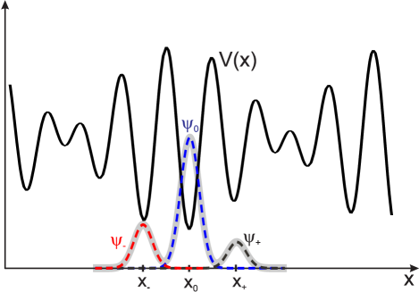
Figure 1: Schematics of the quasi-periodic optical lattice potential $V(x)$ (solid black line) and the triple variational ansatz [Eq. (10)]: the central component $\psi_{0}(x)$ (dashed blue) and satellite ones, $\psi_{+}(x)$ and $\psi_{-}(x)$ (dashed black and red lines, respectively). In the general case, satellites exhibit different peak amplitudes.

We have developed VA for the stationary states using a multi-peak trial function (ansatz, see Appendix A). In this section, we present VA in detail for a three-peak ansatz of the form:

$$\psi(x)=\psi_{0}(x)+\psi_{-}(x)+\psi_{+}(x),$$ (10)

where

$$\psi_{j}(x)=h_{j}\exp\left(-\frac{(x-x_{j})^{2}}{2w_{j}^{2}}\right),$$ (11)

with $h_{j}$ representing amplitudes associated with points $x_{0}$ and $x_{\pm}$, that correspond to local minima of the OL (as illustrated in Fig. 1). In ansatz (10) function $\psi_{0}(x)$ represents the central wave packet, peaking at $x=x_{0}$. We assume that the effective widths of the satellite components $\psi_{-}(x)$ and $\psi_{+}(x)$ are equal to that of the central one, i.e., $w_{+}=w_{-}=w_{0}=w$.

We apply VA only to the overlapping between adjacent peaks, thus focusing on products of the form $\psi_{0}\psi_{j}$. Terms involving $\psi_{+}\psi_{-}$ are neglected as the integrals corresponding overlap integrals are negligibly small. Therefore, the density distribution and interaction-energy density are approximated by

$$|\psi|^{2}\approx\psi_{0}^{2}+\psi_{+}^{2}+\psi_{-}^{2}+2\psi_{0}(\psi_{+}+\psi_{-}),$$ (12)

$$|\psi|^{4}\approx\psi_{0}^{4}+\psi_{+}^{4}+\psi_{-}^{4}+6\psi_{0}^{2}(\psi_{+}^{2}+\psi_{-}^{2})$$ (13)

$$+4\psi_{0}[\psi_{0}^{2}(\psi_{+}+\psi_{-})+\psi_{+}^{3}+\psi_{-}^{3}].$$ (14)

In the framework of VA, one obtains the norm (scaled number of particles in the BEC) as

$$N=\int\limits_{-\infty}^{{+\infty}}|\psi|^{2}dx=\sqrt{\pi}wh_{0}^{2}f_{N}(b_{+},b_{-},w),$$ (15)

where

$$f_{N}(b_{+},b_{-},w)=1+b_{+}^{2}+b_{-}^{2}+2[\varepsilon_{+}(w)b_{+}+\varepsilon_{-}(w)b_{-}],$$ (16)

$$\varepsilon_{\pm}(w)=\exp\left[-\frac{(x_{0}-x_{\pm})^{2}}{4w^{2}}\right],$$ (17)

$b_{\pm}=h_{\pm}/h_{0}$ being ratios of the amplitude of the left and right satellite peaks to the amplitude of the central one. Utilizing Eq. (15), the amplitude in the central peak, $h_{0}$, can be expressed in terms of $N$. Consequently, for a fixed $N$, we have three variational parameters: the common width of the peaks, $w$, and two relative amplitudes of the satellites, $b_{\pm}$.

The energy functional for stationary FNLSE (9) is

$$E=\frac{1}{2}\int\limits_{-\infty}^{{+\infty}}dx\,\psi^{\ast}\left(-\frac{\partial^{2}}{\partial x^{2}}\right)^{\alpha/2}\psi$$

$$+\frac{g}{2}\int\limits_{-\infty}^{{+\infty}}dx\left|\psi\right|^{4}+\int\limits_{-\infty}^{{+\infty}}dxV(x)\left|\psi\right|^{2}.$$ (18)

Employing ansatz Eq. (10), we can analytically calculate all integrals in Eq. (18). In particular,the contribution from the nonlinear self-interaction is linked to the integral

$$\int\limits_{-\infty}^{{+\infty}}|\psi|^{4}dx=\sqrt{\frac{\pi}{2}}wh_{0}^{4}f_{g}(b_{+},b_{-},w),$$ (19)

where

$$f_{g}(b_{+},b_{-},w)=1+b_{+}^{4}+b_{-}^{4}+6\left(\varepsilon_{-}^{2}(w)b_{-}^{2}+\varepsilon_{+}^{2}(w)b_{+}^{2}\right)$$

$$+4\left(b_{-}(1+b_{-}^{2})\varepsilon_{-}^{3/2}(w)+b_{+}(1+b_{+}^{2})\varepsilon_{+}^{3/2}(w)\right).$$ (20)

The OL contribution is expressed in terms of the following integral:

$$\int\limits_{-\infty}^{+\infty}\sin^{2}(\kappa x)|\psi(x)|^{2}dx=\frac{1}{2}\sqrt{\pi}wh_{0}^{2}f_{\kappa}(b_{+},b_{-},w),$$ (21)

where

$$f_{\kappa}(b_{+},b_{-},w)=\sigma_{\kappa}(2\kappa x_{0},w)+\sigma_{\kappa}(2\kappa x_{+},w)b_{+}^{2}$$

$$+\sigma_{\kappa}(2\kappa x_{-},w)b_{-}^{2}+2\varepsilon_{+}(w)\sigma_{\kappa}(\kappa[x_{0}+x_{+}],w)b_{+}$$

$$+2\varepsilon_{-}(w)\sigma_{\kappa}(\kappa[x_{0}+x_{-}],w)b_{-}$$ (22)

and

$$\sigma_{\kappa}(\xi,w)=1-e^{-\kappa^{2}w^{2}}\cos(\xi).$$ (23)

The fractional-diffraction term is actually given by the multiple integral,

$$\int\limits_{-\infty}^{{+\infty}}dx\,\psi^{\ast}\left(-\frac{\partial^{2}}{\partial x^{2}}\right)^{\alpha/2}\psi=\int\limits_{-\infty}^{{+\infty}}dk\,k^{\alpha}\left|\mathcal{F}[\psi]\right|^{2}$$

$$=\frac{\sqrt{\pi}h_{0}^{2}}{2w}f_{\alpha}(b_{+},b_{-},w),$$ (24)

where $\mathcal{F}$ is the symbol of the Fourier transform, cf. Eq. (3),

$$f_{\alpha}(b_{+},b_{-},w)=\frac{2}{\sqrt{\pi}}w^{2-\alpha}\Gamma\left(\frac{1+\alpha}{2}\right)\left\{1+b_{+}^{2}+b_{-}^{2}\right.$$

$$\left.+2b_{+}\chi_{+}\left(\alpha,w\right)+2b_{-}\chi_{-}\left(\alpha,w\right)\right\}$$ (25)

and

$$\chi_{\pm}(\alpha,w)=_{1}F_{1}\left(\frac{1+\alpha}{2},\frac{1}{2},-\frac{(x_{0}-x_{\pm})^{2}}{4w^{2}}\right),$$ (26)

${}_{1}F_{1}(a,b,z)$ being the Kummer’s confluent hypergeometric function. For $\alpha=2$, function $f_{\alpha}$ in Eq. (25) can be expressed in terms of elementary functions, using a known property of the hypergeometric function: ${}_{1}F_{1}(3/2,1/2,z)=e^{z}(1+2z)$ and $\Gamma(3/2)=\sqrt{\pi}/2$.

Finally, we obtain the total VA energy functional:

$$E(b_{+},b_{-},w)=\frac{N}{4w^{2}}I_{\alpha}+\frac{gN^{2}}{2w\sqrt{2\pi}}I_{g}$$

$$+\frac{N}{2}\left(A_{1}I_{V}^{(1)}+A_{2}I_{V}^{(2)}\right),$$ (27)

where $I_{\alpha}$, $I_{g}$, and $I_{V}^{(j)}$ are functions of three variational parameters, $b_{+}$, $b_{-}$, and $w$, defined as follows:

$$I_{\alpha}=f_{\alpha}/f_{N},I_{g}=f_{g}/f_{N}^{2},I_{V}^{(j)}=f_{\kappa_{j}}/f_{N}.$$ (28)

In the limit case of the non-fractional diffraction ($\alpha=2$) and for single-peak ansatz, with $b_{\pm}=0$, energy functional (18) carries over into the one obtained by means of VA in Ref. [26].

Maintaining the normalization condition $N=1$ for fixed LI $\alpha$, and fixed values of the normalized interaction strength $g$ and OL parameters, such as the positions of potential-trap minima ($x_{0},x_{\pm}$), amplitudes ($A_{1},A_{2}$), and $\kappa_{1},\kappa_{2}$ (see Eq. (7)), we aim to find values of the variational parameters $b_{+},b_{-},w$ that minimize energy $E(b_{+},b_{-},w)$.

Further, the density profiles for fixed values of $g=1$, $g=-0.5$ and different values of LI $\alpha$ are plotted in Fig. 2. The peaks tend to narrow with the decrease of $\alpha$, which is explained by the fact that sharper profiles are necessary to balance the nonlinearity in the case of weaker diffraction. Note that, in the cases of $\alpha=1$ and $\alpha<1$ (such as $\alpha=0.8$, shown in Fig. 2), combined with the self-attraction ($g<0$), soliton solutions produced by the 1D FNLSE are unstable, severally, against the action of the critical and supercritical collapse [8, 9].

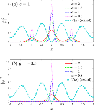
Figure 2: The VA solutions for the three-peak ansatz, obtained in the case of fixed $g=1$ (a) and $g=-0.5$ (b) (the self-repulsive and self-attractive nonlinearities, respectively) and different values of LI ($\alpha$).

Using the VA solutions, we derive the chemical potential $\mu$ as a function of the interaction strength $g$ under fixed normalization $N=1$. Figure 3 illustrates the dependence of the chemical potential and energy on $g$ for the fixed value of the LI, $\alpha=1.5$, comparing results from the VA and numerical methods. Similarly, Fig. 4 compares the form factor given by Eq.(29). The VA based on the three-peak ansatz (10) yields highly accurate results, while the single-peak ansatz performs significantly worse.

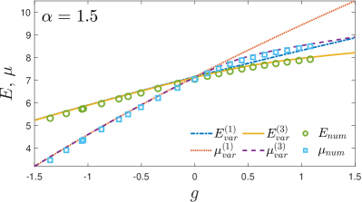
Figure 3: Numerical results (circles and squares) and their VA-produced counterparts, obtained by means of the ansatz admitting the single or three peaks (the dashed and solid lines, respectively), for the dependence of energy $E$ and chemical potential $\mu$ on the coupling constant $g$, for LI $\alpha=1.5$.

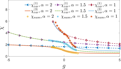
Figure 4: Numerical results and their VA-produced counterparts, obtained by means of the ansatz admitting the single or three peaks, for the dependence of the form-factor ($\chi$, see Eq. (29)) on the coupling constant $g$, for different values of LI: $\alpha=2$, $\alpha=1.5$ and $\alpha=1$.

To characterize the localization degree of the bound states, we define the integral form-factor $\chi$, fixing the normalization condition (6):

$$\chi=\int\limits_{-\infty}^{+\infty}|\psi|^{4}dx.$$ (29)

Larger values of the form-factor correspond to stronger localization. The results produced by VA for the form-factor are summarized by the heatmap in the plane of the nonlinearity strength (coupling constant, $g$) and LI $\alpha$ in Fig. 5.

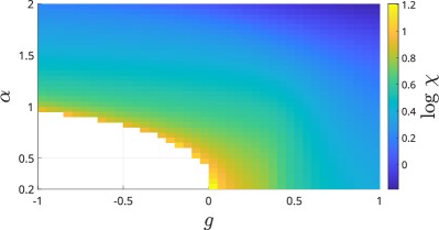
Figure 5: VA results for three-peak states, which display the dependence of the form-factor ($\chi$, see Eq. (29)) on the coupling constant $g$ and LI $\alpha$. VA produces no solutions in the white area.

Next, we consider two-peak in-phase and out-of-phase states (with the same or opposite signs of the peaks of the wave function, respectively). The location of the ansatz’s peaks is $x_{0}\approx 8$ and $x_{1}\approx 9$, where depths of the potential wells take close values.

To identify local energy minima which can produce the VA solutions, we plot the dependence of the energy on the variational parameters $w$ (width) and $b=h_{1}/h_{0}$ (relative amplitude, see Eq. (11)) in Fig. 6. It is seen that, for large enough values of $|g|$, there are two local minima, instead of one. There exist critical values $g_{+}>0$ and $g_{-}<0$, which depend on the LI $\alpha$, such that for $g>g_{+}$ we have out-of-phase solutions, with $h_{1}/h_{0}<0$ (in addition to regular ones with $h_{1}/h_{0}>0$), as seen in panel (a) of Fig. 6. For $g<g_{-}$, panel (b) also exhibits two solutions, with broken symmetry between the two potential wells ($h_{1}/h_{0}<1$ and $h_{1}/h_{0}>1$). Actually, spontaneous symmetry breaking is a well-known property of NLSE solutions with two-well potentials and self-attractive nonlinearity [31, 32].

It is worth noting that, unlike the case of the truly symmetric double-well potential [37], states with broken symmetry below the critical value $g_{-}$ do not emerge from a single point at $h_{1}/h_{0}=1$, and the product of their relative amplitudes is less than 1. Additionally, the absolute value of the relative amplitude $|h_{1}/h_{0}|$ of solutions that exist for $g>g_{-}$ (in particular, out-of-phase states, which appear above $g_{+}$) is less than 1, in contrast to the case of the symmetric potential, where this value is exactly 1. More detailed results for states in the symmetric potential are provided in the Supplemental Material of this article.

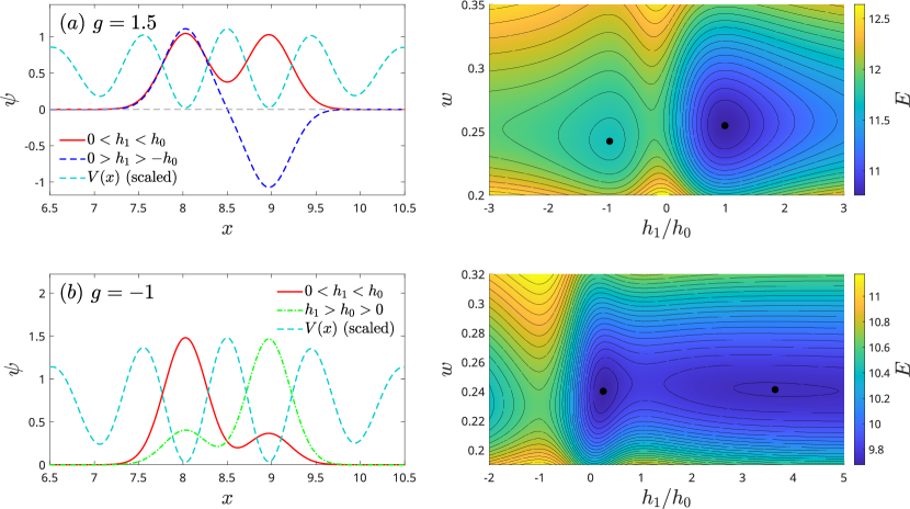
Figure 6: Variational results illustrating the wave function profiles (left) and color-coded energy $E$ (right), given by Eq. (27), as functions of the variational parameters $w$ and $b=h_{1}/h_{0}$, for $\alpha=2$. Panels (a) and (b) correspond to self-repulsive ($g=1.5$) and attractive ($g=-1$) nonlinearities, respectively. Local energy minima are indicated by black dots. The red solid line represents in-phase solutions with $0<h_{1}/h_{0}<1$, the blue dashed line denotes spatially antisymmetric (out-of-phase) solutions with $h_{1}/h_{0}<0$, and the green dash-dotted line indicates a second solution with broken symmetry ($h_{1}/h_{0}>1$).

Properties of the VA-predicted two-peak states are further illustrated by Fig. 7, in which panel (a) shows the relative height of the peaks of the wave function in the bound states vs. $g$, and (b) shows the critical values $g_{\pm}$ vs. LI $\alpha$. It is seen that the critical values become closer to zero with the decrease of $\alpha$, which is explained by the fact that weaker nonlinearity is required to initiate the spontaneous symmetry breaking in the competition with weaker diffraction (corresponding to smaller $\alpha$). It is worthy to note that values $g_{+}$ and $\left|g_{-}\right|$ are quite close for all values of LI $\alpha$.

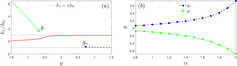
Figure 7: (a) The variational parameter, the peak-amplitude ratio $b=h_{1}/h_{0}$, as the function of the coupling constant, $g$, in the case of the non-fractional diffraction ($\alpha=2$) and normalization $N=1$. (b) The dependence of the critical values of the coupling constant, $g_{+}$ and $g_{-}$ on LI $\alpha$. The second (spatially antisymmetric, out-of-phase) solution, with $h_{1}/h_{0}<0$ (blue dashed lines in both panels), appears at $g>g_{+}$, and the second solution with broken symmetry ($h_{1}/h_{0}>1$, green dash-dotted lines in both panels) appears at $g<g_{-}$. The red solid line indicates the in-phase solutions with $0<h_{1}/h_{0}<1$.

III.2 Numerical solutions

To find stationary solutions numerically, we used a dissipative version of FNLSE (5), including an artificial damping parameter $0<\gamma\ll 1$:

$$(i-\gamma)\,\frac{\partial\widetilde{\Psi}}{\partial t}=\frac{1}{2}\left(-\frac{\partial^{2}}{\partial x^{2}}\right)^{\alpha/2}\widetilde{\Psi}+V(x)\widetilde{\Psi}+\widetilde{g}|\widetilde{\Psi}|^{2}\widetilde{\Psi}-\mu\widetilde{\Psi}.$$ (30)

We use the damped version of GPE to find stationary states rather than to describe some physical dissipative process [33]. Thus, simulating Eq. (30) with the VA-predicted initial condition, it is possible to achieve a numerically accurate stationary state corresponding to chemical potential $\mu$. Although the norm of the wave function and energy are not conserved in the course of the evolution governed by Eq. (30), the wave function eventually converges to a stationary state corresponding to chemical potential $\mu$. The simulations pulled up when the integral residual, defined as

$$\delta\Psi=\int\limits_{-\infty}^{+\infty}\left|\left[\left(-\frac{\partial^{2}}{\partial x^{2}}\right)^{\alpha/2}+V+g|\Psi|^{2}-\mu\right]\Psi\right|^{2}dx,$$ (31)

attained its minimum at some point in time, $t$ $=$ $t_{0}$. Having obtained the stationary state, we renormalized the wave function and the coupling constant as follows:

$$\psi=\widetilde{\Psi}(x,t_{0})/\sqrt{\widetilde{N}},~{}g=\widetilde{g}\widetilde{N},$$ (32)

where $\widetilde{N}$ is the norm of the wave function at $t=t_{0}$, to restore the adopted normalization, $N=1$.

We have compared numerical results generated by means of Eq. (30) and with the help of the above-mentioned ITP method. The latter method produces the same solutions for small $g$, but when $g>0$ increases, the ITP iterative process converges poorly, as the wave function spreads over a large spatial domain. Therefore, we mainly followed the approach based on Eq. (30), as it provides reliable convergence.

IV Dynamics of solitons

The robustness of the bound states was examined by simulations of their evolution. First, Fig. 8 shows the obvious difference in the evolution of the numerical solutions in the linear model ($g=0$ in Eq. (5)) with the periodic and quasiperiodic OL potentials, in the case of the non-fractional diffraction $\alpha=2$. In accordance with the commonly known principles, the wave function spreads out in the former case, and remains confined, due to the AL effect, in the latter situation.

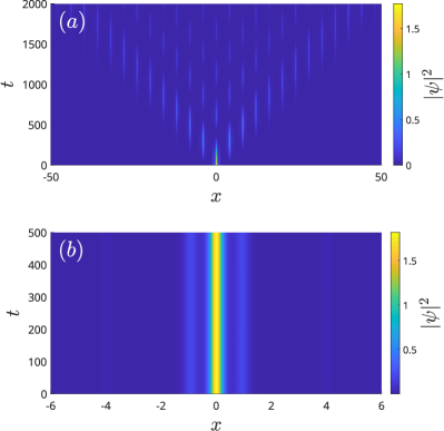
Figure 8: The evolution of three-peak numerical solutions in the linear model with the non-fractional diffraction normal diffraction ($g=0,\alpha=2$), under the action of the periodic (a) and quasiperiodic (b) OL potentials.

On the other hand, it is shown in Fig. 9 that, under the action of the repulsive self-interaction and non-fractional diffraction ($\alpha=2$), not only the quasiperiodic potential but also the periodic one make it possible to create stable localized states – actually, as gap solitons.

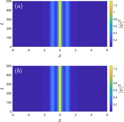
Figure 9: The evolution of the three-peak numerical solutions in the case of the self-repulsion and normal (non-fractional) diffraction ($g=1,\alpha=2$), with norm $N=1$, under the action of the periodic (a) and quasiperiodic (b) OL potentials.

In the case of the fractional diffraction ($\alpha<2$), with the same strength of the self-repulsion (coupling constant), $g=1$, the bound states demonstrate similar robustness. Next, we address FNLSE with stronger repulsive interaction ($g=5$), as in this case Fig. 10 exhibits a difference in the stability between different values of LI $\alpha$. Furthermore, we here produce the results for five-peak bound states, in order to explore the robustness of more complex bound states. It is seen that the bound states are  notably more stable for the fractional diffraction, with $\alpha<2$.

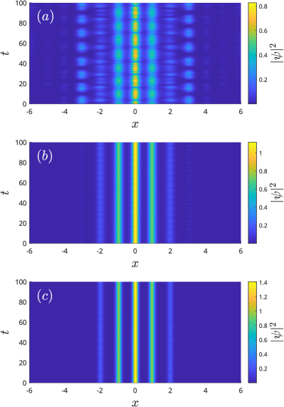
Figure 10: The evolution of the five-peak numerical solutions in the case of the strong self-repulsion ($g=5$) and different values of LI $\alpha$, with norm $N=1$. (a) $\alpha=2$, (b) $\alpha=1.5$, (c) $\alpha=1$.

While the results displayed in Figs. 9, 10, and 10 were obtained in the fully numerical form, it is also relevant to check the evolution of the VA-predicted three-peak modes. It is seen in Fig. 11 that, under the action of the fractional diffraction, with $\alpha=1.5$ and, especially, $\alpha=1$, the ensuing dynamics is essentially more steady than in the case of the non-fractional diffraction, $\alpha=2$, i.e., the VA accuracy improves with the decrease of $\alpha$.

Figure 11: The evolution of the three-peak VA-predicted solutions under the action of strong self-repulsion ($g=5$) and different values of LI $\alpha$, with norm $N=1$. (a) $\alpha=2$, (b) $\alpha=1.5$, (c) $\alpha=1$.

V Conclusion

We have investigated the interplay between the fractional diffraction and 1D quasiperiodic potentials in shaping the gap-soliton dynamics. Using the VA (variational approximation) and numerical methods, we have produced self-trapped states and identified their stability, varying the LI (Lévy index) which determines the fractional diffraction. These findings not only advance the understanding of the nonlinear wave propagation in fractional and disordered media but also expand potential applications of solitons in optical data-processing schemes, by revealing conditions for improving the stability of the solitons.

It is relevant to extend the analysis for the compound states including two or several localized modes considered above. Promising possibilities are to consider the interplay of the fractional diffraction with other forms of nonlinearity (in particular, nonpolynomial terms [34, 35], which are produced by strong confinement applied to BEC in the transverse directions) and, eventually, higher-dimensional settings. In particular, it may be interesting to construct two- and three-dimensional localized modes with embedded vorticity.

Appendix A Generalized variational analysis

Here we present calculations of the integrals with the multi-peak ansatz:

$$\psi=\sum_{j}h_{j}\exp\left(-\frac{(x-x_{j})^{2}}{2w^{2}}\right).$$ (33)

The corresponding energy functional is:

$$E=\int\limits_{-\infty}^{+\infty}dx\left[\psi^{*}\,\frac{1}{2}\left(-\frac{\partial^{2}}{\partial x^{2}}\right)^{\alpha/2}\psi+V(x)|\psi|^{2}+\frac{g}{2}\,|\psi|^{4}\right]$$

$$=\frac{1}{2\pi}\int\limits_{0}^{+\infty}p^{\alpha}|\mathcal{F}\psi|^{2}dp+\sum_{i=1}^{2}A_{i}\int\limits_{-\infty}^{+\infty}\sin^{2}\left(\kappa_{i}x\right)|\psi|^{2}dx$$

$$+\frac{g}{2}\int\limits_{-\infty}^{+\infty}|\psi|^{4}dx,$$ (34)

where $\mathcal{F}$ is the symbol of the Fourier transform. We consider only the overlapping between neighboring peaks, denoting $b_{j}=h_{j}/h_{0}$, where $h_{0}$ is the amplitude of one of the peaks (for instance, the central one). We have variational parameters $w$ and $\{b_{j\neq 0}\}$, whose total number is equal to the number of peaks. For the norm of the ansatz we obtain

$$N=\int\limits_{-\infty}^{+\infty}|\psi|^{2}dx$$

$$=\sum_{j,k}h_{j}h_{k}\int\limits_{-\infty}^{+\infty}\exp\left(-\frac{(x-x_{j})^{2}+(x-x_{k})^{2}}{2w^{2}}\right)dx$$

$$=\sum_{j,k}\left\{h_{j}h_{k}\exp\left(-\frac{(x_{j}-x_{k})^{2}}{4w^{2}}\right)\right.$$

$$\left.\times\int\limits_{-\infty}^{+\infty}\exp\left[-\frac{1}{w^{2}}\left(x-\frac{x_{j}+x_{k}}{2}\right)^{2}\right]dx\right\}$$

$$=\sqrt{\pi}w\sum_{j,k}h_{j}h_{k}\varepsilon_{jk}(w)=\sqrt{\pi}wh_{0}^{2}f_{N},$$ (35)

where

$$f_{N}=1+\sum_{j\neq 0}b_{j}^{2}+2\sum_{\langle j,k\rangle}b_{j}b_{k}\varepsilon_{jk}(w),$$ (36)

$$\varepsilon_{jk}(w)=\exp\left(-\frac{(x_{j}-x_{k})^{2}}{4w^{2}}\right)$$ (37)

and $\displaystyle\sum_{\langle j,k\rangle}$ denotes the sum over the neighboring indices. By fixing norm $N$, we can eliminate $h_{0}$:

$$h_{0}^{2}=\frac{N}{\sqrt{\pi}wf_{N}}.$$ (38)

The corresponding kinetic-energy term is

$$\frac{1}{2\pi}\int\limits_{0}^{+\infty}p^{\alpha}|\mathcal{F}\psi|^{2}dp$$

$$=\frac{1}{2\pi}\int\limits_{0}^{+\infty}p^{\alpha}\left|\sum_{j}h_{j}\int\limits_{-\infty}^{+\infty}\exp\left(-\frac{(x-x_{j})^{2}}{2w^{2}}\right)e^{-ipx}dx\right|^{2}dp$$

$$=\frac{1}{2\pi}\int\limits_{0}^{+\infty}p^{\alpha}\left|\sum_{j}h_{j}e^{-ipx_{j}}\sqrt{2\pi}we^{-p^{2}w^{2}/2}\right|^{2}dp$$

$$=w^{2}\sum_{j,k}h_{j}h_{k}\int\limits_{0}^{+\infty}p^{\alpha}e^{-p^{2}w^{2}}\cos\Big{(}p(x_{j}-x_{k})\Big{)}dp$$

$$=\frac{\Gamma\left(\frac{\alpha+1}{2}\right)}{2w^{\alpha-1}}\sum_{j,k}h_{j}h_{k}\chi_{jk}^{(\alpha)}(w)=\frac{\Gamma\left(\frac{\alpha+1}{2}\right)N}{2\sqrt{\pi}w^{\alpha}}\,\frac{f_{K}}{f_{N}},$$ (39)

where

$$f_{K}=1+\sum_{j\neq 0}b_{j}^{2}+2\sum_{\langle j,k\rangle}b_{j}b_{k}\chi_{jk}^{(\alpha)}(w),$$ (40)

$$\chi_{jk}^{(\alpha)}(w)=\,_{1}F_{1}\left(\frac{\alpha+1}{2},\frac{1}{2},-\frac{(x_{j}-x_{k})^{2}}{4w^{2}}\right).$$ (41)

The potential-energy term:

$$\sum_{i=1}^{2}A_{i}\int\limits_{-\infty}^{+\infty}\sin^{2}\left(\kappa_{i}x\right)|\psi|^{2}dx$$

$$=\sum_{i=1}^{2}A_{i}\sum_{j,k}\left\{h_{j}h_{k}\varepsilon_{jk}(w)\int\limits_{-\infty}^{+\infty}\sin^{2}(\kappa_{i}x)\right.$$

$$\left.\times\exp\left[-\frac{1}{w^{2}}\left(x-\frac{x_{j}+x_{k}}{2}\right)^{2}\right]dx\right\}$$

$$=\frac{\sqrt{\pi}w}{2}\sum_{i=1}^{2}A_{i}\sum_{j,k}h_{j}h_{k}\varepsilon_{jk}(w)\sigma_{jk}^{(i)}(w)$$

$$=\frac{N}{2f_{N}}\sum_{i=1}^{2}A_{i}f_{P}^{(i)},$$ (42)

where

$$f_{P}^{(i)}=\sigma_{00}^{(i)}(w)+\sum_{j\neq 0}b_{j}^{2}\sigma_{jj}^{(i)}(w)$$

$$+2\sum_{\langle j,k\rangle}b_{j}b_{k}\varepsilon_{jk}(w)\sigma_{jk}^{(i)}(w),$$ (43)

$$\sigma_{jk}^{(i)}(w)=1-e^{-\kappa_{i}^{2}w^{2}}\cos\Big{(}\kappa_{i}(x_{j}+x_{k})\Big{)}.$$ (44)

The interaction-energy term:

$$\frac{g}{2}\int\limits_{-\infty}^{+\infty}|\psi|^{4}dx=\frac{g}{2}\sum_{j_{1},j_{2},j_{3},j_{4}}\left\{\left(\prod_{k=1}^{4}h_{j_{k}}\right)\right.$$

$$\left.\times\int\limits_{-\infty}^{+\infty}\exp\left(-\frac{1}{2w^{2}}\sum_{k=1}^{4}(x-x_{j_{k}})^{2}\right)dx\right\}$$

$$=\frac{\sqrt{\pi}gw}{2\sqrt{2}}\sum_{j_{1},j_{2},j_{3},j_{4}}\Bigg{\{}\left(\prod_{k=1}^{4}h_{j_{k}}\right)$$

$$\left.\times\exp\left[-\frac{1}{2w^{2}}\left(\sum_{k=1}^{4}x_{j_{k}}^{2}-\frac{1}{4}\left(\sum_{k=1}^{4}x_{j_{k}}\right)^{2}\right)\right]\right\}$$

$$\frac{gN^{2}}{2\sqrt{2\pi}w}\,\frac{f_{I}}{f_{N}^{2}},$$ (45)

where

$$f_{I}=1+\sum_{j\neq 0}b_{j}^{4}+4\sum_{\langle j,k\rangle}b_{j}b_{k}\left(b_{j}^{2}+b_{k}^{2}\right)\varepsilon_{jk}^{3/2}(w)$$

$$+6\sum_{\langle j,k\rangle}b_{j}^{2}b_{k}^{2}\varepsilon_{jk}^{2}(w).$$ (46)

We thus obtain the expression for the total energy accounting on the interaction between neighboring sites:

$$E=\frac{\Gamma\left(\frac{\alpha+1}{2}\right)N}{2\sqrt{\pi}w^{\alpha}}\,\frac{f_{K}}{f_{N}}+\frac{N}{2f_{N}}\sum_{i=1}^{2}A_{i}f_{P}^{(i)}+\frac{gN^{2}}{2\sqrt{2\pi}w}\,\frac{f_{I}}{f_{N}^{2}}$$

$$=\frac{N}{2f_{N}}\left[\frac{\Gamma\left(\frac{\alpha+1}{2}\right)}{\sqrt{\pi}w^{\alpha}}\,f_{K}+\sum_{i=1}^{2}A_{i}f_{P}^{(i)}\right.$$

$$\left.+\frac{gN}{\sqrt{2\pi}w}\,\frac{f_{I}}{f_{N}}\right].$$ (47)

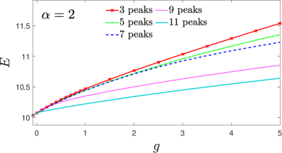
Figure 12: The VA results for the dependence of energy $E$ (see Eq. (47)) on the coupling constant $g>0$ (self-repulsion) for ansatz with different numbers of peaks (see Eq. (A1)) under normalization $N=1$, in the case of normal diffraction $(\alpha=2)$.

In Fig. 12 we see that ansatz with a greater number of peaks produce lower energy for a fixed value of the coupling constant $g$. This property reflects the fact that every additional peak increases the number of degrees of freedom of the trial function and thus gives an option to reduce the predicted value of the energy functional.

Figure 13 shows that, as coupling constant $g>0$ increases (in the case of the self-repulsion), the form-factor $\chi$ decreases for each fixed number of peaks of the ansatz, signifying the growth of the satellite peaks.

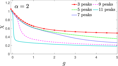
Figure 13: The VA results for ansatz with different numbers of peaks, which produce the dependence of the form-factor $\chi$, see Eq. (29), on the coupling constant $g>0$ in the case of normal diffraction $\alpha=2$ and normalization $N=1$.

Supplemental Material

A.1 Two-hump states in periodic potential

Here we present the results of the variational analysis (VA) with two-peak ansatz for the specific case of periodic potential with $A_{2}=0$ in Eq. (4). As expected, the results for the periodic potential are very similar to the properties of the in-phase, out-of-phase symmetric and asymetric solutions previously investigated in Refs. [36, 37] for the symmetric double-well potential.

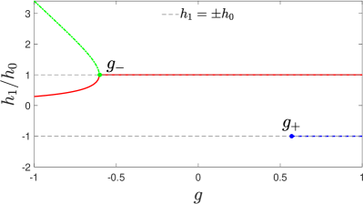
Figure 14: The VA-predicted dependence of the peak-amplitude ratio ($b=h_{1}/h_{0}$) on coupling constant $g$ in the case of the non-fractional diffraction ($\alpha=2$) and normalization $N=1$ in the periodic potential. The second (spatially antisymmetric) solution, with $h_{1}/h_{0}<0$ (blue dashed line), appears at $g>g_{+}$, and the second solution with broken symmetry ($h_{1}/h_{0}>1$, green dash-dotted line) appears at $g<g_{-}$.

As shown in Fig. 14, the symmetric in-phase state (red curve) with $h_{1}/h_{0}=1$ bifurcates into two asymmetric in-phase states (green and red curves) for $g<g_{-}$. Notably, the product of the ratios $(h_{1}/h_{0})$ for these two branches equals unity, consistent with the preservation of mirror symmetry in the two-hump states of the potential.

The energy landscapes in the plane of the two variational parameters are depicted for different values of nonlinearity strength $g$, near the bifurcation points $g_{-}$ and $g_{+}$, in Fig. 15 and Fig. 16, respectively.

Notably, the energy minima that correspond to the out-of-phase solutions are significantly less deep than the ones for the in-phase solutions, both in cases of periodic and quasiperiodic potentials (Fig. 15). Thus, from this energetic analysis follows that the out-of-phase solitons should be less robust than the in-phase states. These predictions are supported by our numerical simulation of the soliton dynamics. Also, the second solution with broken symmetry (with $h_{1}/h_{0}>1$) has greater energy than the first one (with $h_{1}/h_{0}<1$) in the case of the quasiperiodic lattice, in contrast to the periodic one, where respective energies are the same (see Supplemental Materials), which reflects the fact that the second potential minimum has lower depth than the first one.

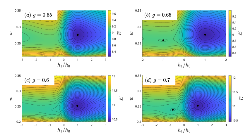
Figure 15: The VA results illustrating the appearance of the second local minimum of energy $E$ (see Eq. (LABEL:eq:E_var_Npeaks)) in the case of the non-fractional diffraction ($\alpha=2$) for the self-repulsive nonlinearity near the critical value $g_{+}$. Local energy minima are marked by black dots. (a), (b) periodic potential; (c), (d) quasiperiodic potential.

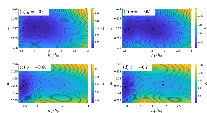
Figure 16: The VA results illustrating the appearance of the second local minimum of energy $E$ (see Eq. (LABEL:eq:E_var_Npeaks)) in the case of the non-fractional diffraction ($\alpha=2$) for the self-attractive nonlinearity near the critical value $g_{-}$. Local energy minima are marked by black dots. (a), (b) periodic potential; (c), (d) quasiperiodic potential.

A.2 Additional variational results

We now discuss the application of the variational method developed in this work to the well-studied case of a quasiperiodic lattice with non-fractional diffraction, $\alpha=2$. The density profiles of the so-obtained VA solutions (bound states) are plotted, for different values of coupling constant (nonlinearity coefficient) $g$, in Fig. 17. As expected, the height of the side peaks increases with the increase of $g$ when repulsive interaction essentially modifies the soliton shape. In the limit of the strong repulsion (large $g$), the bound states are well approximated by the Thomas-Fermi approximation, which neglects the diffraction term and, therefore, is not affected by the value of the $\alpha$ (this limit case is a well-known one, therefore it is not presented here in detail).

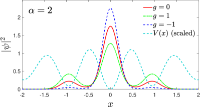
Figure 17: Density profiles for the VA solutions for the three-peak ansatz for different values of the normalized coupling constant ($g$), in the case of the normal (non-fractional) diffraction, $\alpha=2$.

Figure 18 shows the comparison of the single- and three-peak VA solutions to the numerical one, obtained by means of the imaginary-time propagation method (ITP) [29, 30], for the non-interacting condensate ($g=0$). Good agreement is observed between the three-peak VA solution and the numerical one.

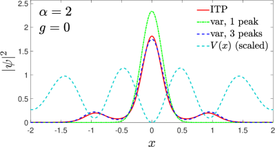
Figure 18: VA solutions for single- and three-peak ansätze, compared to the numerical solution, for the non-interacting condensate with normal diffraction $(g=0,\alpha=2)$.

The consistency between numerical and three-peak variational solutions is further illustrated in Fig. 19 using such integral characteristics as energy ($E$) and chemical potential ($\mu$). It is evident that for lower values of the Lévi index $\alpha$, the single-peak ansatz yields sufficient accuracy over a broad range of coupling constant values. This reflects the tendency of the wave function to localize on a single lattice site as the diffraction term is suppressed with decreasing $\alpha$.

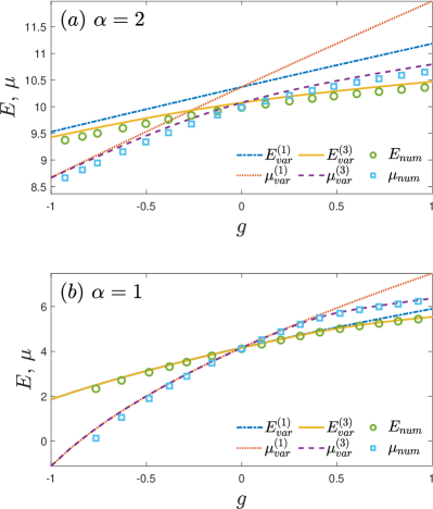
Figure 19: Numerical results (circles and squares) and their VA-produced counterparts, obtained by means of the ansatz admitting the single or three peaks (the dashed and solid lines, respectively), for the dependence of energy $E$ and chemical potential $\mu$ on the coupling constant $g$, for different values of LI: (a) $\alpha=2$ and (b) $\alpha=1$.

References

- [1] N. Laskin, Fractional quantum mechanics and Lévy path integrals, Phys. Lett. A 268, 298-305 (2000).
- [2] N. Laskin, Fractional quantum mechanics (World Scientific: Singapore, 2018).
- [3] B. B. Mandelbrot, The Fractal Geometry of Nature (W. H. Freeman, New York, 1982).
- [4] X. Guo and M. Xu, Some physical applications of fractional Schrödinger equation, J. Math. Phys. 47, 082104 (2006).
- [5] M. Cai and C. P. Li, On Riesz derivative, Fract. Calc. Appl. Anal. 22, 287-301 (2019).
- [6] S. Longhi, Fractional Schrödinger equation in optics, Opt. Lett. 40, 1117-1120 (2015).
- [7] S. Liu, Y. Zhang, B. A. Malomed, and E. Karimi, Experimental realisations of the fractional Schrödinger equation in the temporal domain, Nature Communications 14, 222 (2023).
- [8] B. A. Malomed, Optical solitons and vortices in fractional media: A mini-review of recent results, Photonics 8, 353 (2021),
- [9] B. A. Malomed, Basic fractional nonlinear-wave models and solitons, Chaos 34, 022102 (2024).
- [10] X. Ren and F. Deng, Fundamental solitons in optical lattices with fractional-order diffraction, Opt. Commun. 495, 127039 (2021).
- [11] X. Liu, B. A. Malomed, and J. Zeng, Localized modes in nonlinear fractional systems with deep lattices, Advanced Theory and Simulations 2, 100482 (2022).
- [12] X. Yao and X. Liu, Off-site and on-site vortex solitons in space-fractional photonic lattices, Opt. Lett. 43, 5749-5752 (2018).
- [13] B. B. Baizakov, B. A. Malomed, and M. Salerno, Multidimensional solitons in periodic potentials, Europhys. Lett. 63, 642-648 (2003).
- [14] J. Yang and Z. H. Musslimani, Fundamental and vortex solitons in a two-dimensional optical lattice, Opt. Lett. 28, 2094-2096 (2003).
- [15] C. Mejia-Cortes and M. I. Molina, Fractional discrete vortex solitons, Opt. Lett. 46, 2256-2259 (2021).
- [16] C. M. de Sterke and J. E. Sipe, Gap solitons, Prog. Opt., vol. XXXIII, 203-260 (1994).
- [17] V. A. Brazhnyi and V. V. Konotop, Theory of nonlinear matter waves in optical lattices, Mod. Phys. Lett. B 18, 627-651 (2004).
- [18] O. Morsch and M. Oberthaler, Dynamics of Bose-Einstein condensates in optical lattices, Rev. Mod. Phys. 78, 179-212 (2006).
- [19] P. Chatterjee and R, Modak, One-dimensional Lévy quasicrystal, J. Phys.: Condens. Matter 35, 505602 (2023).
- [20] Y. Zhang, X. Liu, M. R. Belić, W. Zhong, Y. Zhang, M. Xiao, Propagation dynamics of a light beam in a fractional Schrödinger equation, Phys. Rev. Lett. 115, 180403 (2015).
- [21] H. Sakaguchi and B. A. Malomed. Gap solitons in quasiperiodic optical lattices, Phys. Rev. E 74, 026601 (2006).
- [22] M. Chen, S. Zeng, D. Lu, W. Hu, and Q. Guo, Optical solitons, self-focusing, and wave collapse in a space-fractional Schrödinger equation with a Kerr-type nonlinearity, Phys. Rev. E 98, 022211 (2018).
- [23] B. A. Malomed, Multidimensional Solitons (American Institute of Physics: Melville, NY, 2022).
- [24] Y. Lahini, A. Avidan, F. Pozzi, M. Sorel, R. Morandotti, D. N. Christodoulides, and Y. Silberberg, Anderson localization and nonlinearity in one-dimensional disordered photonic lattices, Phys. Rev. Lett. 100, 013906 (2009).
- [25] S. Flach, D. O. Krimer, and Ch. Skokos, Universal spreading of wave packets in disordered nonlinear systems, Phys. Rev. Lett. 102, 024101 (2009).
- [26] S. K. Adhikari and L. Salasnich, Localization of a Bose-Einstein condensate in a bichromatic optical lattice, Phys. Rev. A 80, 023606 (2009).
- [27] H. Sakaguchi and B. A. Malomed, One- and two-dimensional solitons in spin-orbit-coupled Bose-Einstein condensates with fractional kinetic energy, J. Phys. B: At. Mol. Opt. Phys. 55, 155301 (2022).
- [28] C. Huang, C. Li, H. Deng, and L. Dong, Gap Solitons in Fractional Dimensions With a Quasi-Periodic Lattice, Ann. Phys. (Berlin) 2019, 1900056 (2019).
- [29] M. L. Chiofalo, S. Succi, and M. P. Tosi, Ground state of trapped interacting Bose-Einstein condensates by an explicit imaginary-time algorithm, Phys. Rev. E 62, 7438-7444 (2000).
- [30] W. Z. Bao and Q. Du, Computing the ground state solution of Bose-Einstein condensates by a normalized gradient flow, SIAM J. Sci. Comp. 25, 1674-1697 (2004).
- [31] G. J. Milburn, J. Corney, E. M. Wright, and D. F. Walls, Quantum dynamics of an atomic Bose-Einstein condensate in a double-well potential, Phys. Rev. A 55, 4318-4324 (1997).
- [32] A. Smerzi, S. Fantoni, S. Giovanazzi, and S. R. Shenoy, Quantum coherent atomic tunneling between two trapped Bose- Einstein condensates, Phys. Rev. Lett. 79, 4950-4953 (1997).
- [33] S. Choi, S. A. Morgan, and K. Burnett, Phenomenological damping in trapped atomic Bose-Einstein condensates, Phys. Rev. A 57, 4057-4060 (1998).
- [34] L. Salasnich, A. Parola, and L. Reatto, Effective wave equations for the dynamics of cigar-shaped and disk-shaped Bose condensates, Phys. Rev. A 65, 043614 (2002)
- [35] A. Muñoz Mateo and V. Delgado, Effective mean-field equations for cigar-shaped and disk-shaped Bose-Einstein condensates, Phys. Rev. A 77, 013617 (2008).
- [36] T. Mayteevarunyoo, B. A. Malomed, and G. Dong, Spontaneous symmetry breaking in a nonlinear double-well structure, Phys. Rev. A, 78, 053601, (2008).
- [37] B. A. Malomed, Spontaneous symmetry breaking in nonlinear systems: An overview and a simple model, in Nonlinear Dynamics: Materials, Theory and Experiments, Springer Proceedings in Physics, vol. 173, 2016, ed. by M. Tlidi and M. Clerc, pp. 97-112.