An Eccentric Binary with a Misaligned Circumbinary Disk

Abstract

We present spectroscopic and photometric observations of Bernhard-2, which was previously identified as a candidate system to host a misaligned circumbinary disk. Our spectroscopic measurements confirm that Bernhard-2 indeed contains an eccentric ($e=0.69\pm 0.08$) binary and thus that the periodic variability in the photometric light curve is best explained by the occultation by the misaligned circumbinary disk. By modeling the spectral energy distributions at different phases, we infer the system age to be $\sim 20\,$Myr and the masses of the two binary components to be $\sim 1.1\,M_{\odot}$ and $\sim 0.9\,M_{\odot}$, respectively. Our new photometric observations show clear deviations from the model prediction based on the archival data, suggesting ongoing precession of the circumbinary disk. The H$\alpha$ line of Bernhard-2 also shows an inverse P-Cygni profile at epochs close to the pericenter passage, which could be attributed to the pulsed accretion around the pericenter. Bernhard-2 therefore closely resembles the well studied KH 15D system. Further detailed observations and studies of such rare systems can provide useful information about disk physics and evolution.

1 Introduction

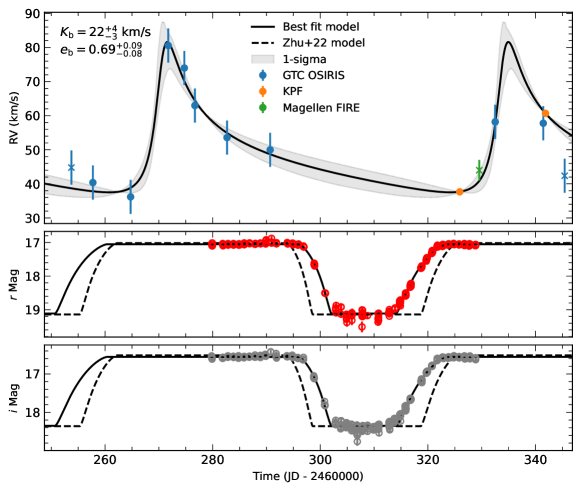
Figure 1: Spectroscopic (top panel) and photometric (middle and bottom panels) measurements of the Bernhard-2 system. The solid line in each panel represents the best-fit model. The grey shaded region in the top panel is the 1-$\sigma$ uncertainty of the RV model. In the top panel, the blue, orange, and green points are the RV measurements from GTC, KPF, and FIRE, respectively. Note that we assume the FIRE data point has the same RV offset with KPF. GTC and FIRE measurements that are not used in the RV modeling are indicated by cross. The new photometric measurements are taken in $r$ (middle panel) and $i$ (bottom panel) bands. The new light curves do not agree with the best-fit model of Zhu et al. (2022), which may suggest some substantial precession of the circumbinary disk.

The discovery of over a dozen circumbinary planets has substantially advanced our understanding of the exoplanet population (e.g., Doyle et al., 2011; Kostov et al., 2020). Although the majority of the circumbinary planets are coplanar to the central binaries, circumbinary objects with misaligned or even polar orbits are predicted to exist, especially around eccentric binaries (e.g., Aly et al., 2015; Martin & Lubow, 2017; Lubow & Martin, 2018; Zanazzi & Lai, 2018; Cuello & Giuppone, 2019; Smallwood et al., 2020). Indeed, some misaligned and even polar circumbinary protoplanetary disks have been detected (e.g., Köhler, 2011; Kennedy et al., 2012; Brinch et al., 2016; Lacour et al., 2016; Fernández-López et al., 2017; Kennedy et al., 2019; Kenworthy et al., 2022), and all exhibit relatively high eccentricity ($e\gtrsim 0.5$).

At intermediate ages, debris disks connect the protoplanetary disk phase and the mature planetary system. Circumbinary debris disks with misaligned orbits relative to the central binaries are difficult to detect. Nevertheless, one well-studied system of this kind is KH 15D (Kearns & Herbst, 1998). Following its discovery via photometric observations, theoretical models were developed to explain the photometric behavior (Winn et al., 2004; Chiang & Murray-Clay, 2004). These models suggest that a misaligned circumbinary disk, combined with the reflex motion of central binary stars, causes the system to show periodically the long and complex dimming events. Shortly after these models were proposed, spectroscopic observations confirmed the binary nature of KH 15D (Johnson et al., 2004).

The unique geometric configuration of the KH 15D system allows for various observational methods to constrain different properties of the system. The system’s light curve, under long-term photometric monitoring, shows complex behavior due to the precession of the disk (Johnson et al., 2005; Maffei et al., 2005; Hamilton et al., 2005; Capelo et al., 2012; Aronow et al., 2018; García Soto et al., 2020). This is useful for probing the disk in detail, including geometry and dynamical constraints (e.g., Winn et al., 2006; Poon et al., 2021) and properties of disk material and substructures (e.g., Silvia & Agol, 2008; Arulanantham et al., 2016; García Soto et al., 2020).

The (nearly) all-sky photometric surveys have enabled the identification of more systems similar to KH 15D (references). In particular, Zhu et al. (2022) reported two candidate systems with KH 15D-like light curves from the Zwicky Transient Facility (ZTF, Bellm et al., 2019; Masci et al., 2019), which they named Bernhard-1 and Bernhard-2. Both objects exhibit dimming of more than 2 magnitudes in multiple bands, lasting over one-third of their periods. These features resemble closely the key characteristics of the KH 15D system. Additionally, both targets show infrared excess in near to mid-infrared bands, suggesting the presence of a cold disk.

In this work, we confirm with spectroscopic observations that the Bernhard-2 system indeed contains an eccentric binary. In Section 2, we describe our new observations and the data reduction procedures. In Section 3, we present the physical interpretations, including modelings of the RV curve and the system SED. Finally, in Section 4, we summarize our results and discuss a few interesting features that deserve future follow-up studies.

2 Observations

2.1 GTC/OSIRIS

We obtained 11 spectra of Bernhard-2 over a time interval of $\sim 92$ days from the OSIRIS instrument (Cepa et al., 2013) installed on the 10.4 m Gran Telescopio CANARIAS (GTC). Observations were taken at random orbital phases during the out-of-occultation windows. A radial velocity standard star, CoRot-7, was also observed following Bernhard-2 in the first three nights in order to test the RV stability. We used the long-slit mode of OSIRIS, with the R2500R grism and a slit width of 0.6$\arcsec$ for both targets. This yields a wavelength coverage from 5575 ${\rm\AA}$ to 7685 ${\rm\AA}$ and a spectral resolution of $\sim 2500$. The exposure times are 900 s and 20 s for Bernhard-2 and CoRot-7, respectively.

The GTC data were reduced with the PypeIt package (Prochaska et al., 2020, 2020) following the standard process. The wavelengths are calibrated by the lamp spectra taken by the same instrument. For each lamp frame, we manually identified strong lines and ignored those with signal-to-noise (S/N) below 20, in order to achieve a robust wavelength solution.

The RV standard star shows an RV variation up to 20 km/s after the wavelength calibration by the lamp spectra, so we also refined the wavelength solution by calibrating the telluric emission lines to the sky spectrum model. In this step, the telluric lines were obtained by PypeIt, and the wavelengths of the sky spectrum model, available on the GTC website were converted from air to vacuum by the airvacuumvald package, in which step the relation in Morton (2000) was used. After this refinement, the RV uncertainty on CoRot-7 was reduced substantially, with a standard deviation of $\sim$3.5 km/s from the absolute RV value of the same star from Gaia DR3 (Gaia Collaboration et al., 2023). Applying the same procedure to Bernhard-2, we obtained a wavelength uncertainty of $\sim$0.1 $\rm\AA$ based on the internal scattering.

We extract the RVs by cross-correlating the wavelength-calibrated stellar spectra with a single-star spectrum template. The template is obtained by interpolating in the Phoenix library (Husser et al., 2013) at the parameter values of the primary star. Motivated by the original spectral analysis of Zhu et al. (2022) and the SED fitting in Section 3.2, we set the primary star parameters to be $T_{\rm eff}=4850\,$K, $\log g=4.5$, and $\rm[Fe/H]=0.4$. The theoretical template is further convoluted to the resolution of ${\rm R}\sim 2500$. Before conducting the cross-correlation, we normalize both the observed and template spectra using iSpec (Blanco-Cuaresma, 2019), and visually confirm that the resulting continua are flat. Additionally, we have removed outliers and excluded certain wavelength ranges that were affected by the atmosphere (e.g., oxygen $\gamma$ band) or the stellar variability (e.g., H$\alpha$; see Section 4). In deriving the RV values we have not considered the impact of the uncertainties in the primary star parameters or the inclusion of the secondary star. The former would only modify the line profiles slightly, and its impact on the derived RVs is negligible. Regarding the impact of the secondary star, this secondary star only contributes $\sim 0.16$ to the total flux in the wavelength range that is considered here (see Section 3.2). We have tested that using a binary spectrum template with such a flux ratio would only change the derived RV values typically by $\lesssim 3\,$km/s, which is comparable to the RV uncertainty from the wavelength calibration. The contribution of photon noise to the final RV error is determined through bootstrapping, yielding an error of $\lesssim 1.5\,$km/s across all epochs. The overall RV uncertainty is set at $5\,$km/s, significantly exceeding the photon-noise-limited error to accommodate potential systematics. The extracted RV measurements are shown in the top panel of Figure 1, and the values are also given in Table 2.

2.2 Other Spectroscopic Measurements

Two spectroscopic observations of Bernhard-2 were obtained from the newly commissioned Keck Planet Finder (KPF, Gibson et al., 2016, 2018, 2020) mounted on the Keck I telescope. KPF is a fiber-fed echelle spectrograph with a spectral resolution of $R\sim 98,000$ and a wavelength coverage from 4450 ${\rm\AA}$ to 8700 ${\rm\AA}$. Both observations had an exposure time of 900 seconds. The spectra were reduced with the KPF Data Reduction Pipeline (DRP) that is publicly available . See also the RV measurement by Dai et al. (2024). Because the KPF pipeline estimates RV error based solely on the photon noise, it tends to underestimate the errors for faint stars such as Bernhard-2. To address this issue, we choose to inflate the RV uncertainties of KPF by approximately a factor of five. Additionally, we have also incorporated an RV jitter term in the modeling, as detailed in Section 3.1.

We have also obtained one spectrum of Bernhard-2 in the near IR with Magellan Folded-port InfraRed Echellette (FIRE; Simcoe et al. 2008) using the echelle mode, which delivers continuous wavelength coverage from $Y$ through $K$ bands (0.82-2.51 microns). The observation was conducted with 1$\arcsec$ width slit under varying seeing between 1.0$\arcsec$ to 1.4$\arcsec$. The FIRE data was reduced with the PypeIt package following the standard procedures. The OH sky emission lines were used for wavelength calibration. The estimated resolution of the result spectrum is $\sim$2500. Using a stellar template with $T_{\rm eff}=4900\,$K, we derive an RV measurement of $44\pm 3\,{\rm km\,s^{-1}}$.

These KPF and FIRE RV measurements are also shown in the top panel of Figure 1.

2.3 Photometric Observations

High-cadence photometric observations of Bernhard-2 were obtained between December 1st, 2023, and January 19th, 2024, when the occultation event was expected to happen. These observations were taken by the 32 inch telescope at the Post Observatory in both $r$ and $i$ bands. As shown in the middle and bottom panels of Figure 1, these new light curves appear different from the prediction of the original photometric model of Zhu et al. (2022), which was based on the sparse ZTF observations, again suggesting that the misaligned circumbinary disk may be undergoing precession. The updated times and projected velocities of both ingress and egress of the occultation event are given in Table 1. Intensive photometric observations like those shown in Figure 1 in the long term will be useful in better constraining the time evolution of such a rare system, as has been demonstrated in the famous KH-15D system (see Poon et al. 2021 and references therein).

3 Physical Interpretation

Table 1: The SED and RV best-fit parameters as well as the inferred properties (marked with ^∗). The subscript $1$ and $2$ indicate the primary and secondary star in the binary, respectively. Here BJD${}^{\prime}=$BJD$-2460000$.

SED fitting
S1 EEP	EEP1	$183\pm 3$
S2 EEP	EEP2	$173\pm 4$
Log of age (yr)	$\log\mathrm{Age}$	$7.3\pm 0.09$
Metallicity	$\mathrm{[Fe/H]}$	$0.46\pm 0.11$
Distance	$d$ (kpc)	$1.82\pm 0.13$
Extinction	$A_{V}$ (mag)	$0.85\pm 0.10$
S1 Mass	$M_{1}^{*}$ ($M_{\odot}$)	$1.13\pm 0.07$
S1 Radius	$R_{1}^{*}$ ($R_{\odot}$)	$1.15\pm 0.08$
S1 Effective Temperature	$T_{\mathrm{eff},1}^{*}$ (K)	$4870\pm 70$
S2 mass	$M_{2}^{*}$ ($M_{\odot}$)	$0.87\pm 0.04$
S2 radius	$R_{2}^{*}$ ($R_{\odot}$)	$1.15\pm 0.08$
S2 Effective Temperature	$T_{\mathrm{eff},2}^{*}$ (K)	$3990\pm 40$
RV fitting
Periastron time	$T_{P1}$ (BJD′)	$270.5\pm 0.8$
Eccentricity	$e$	$0.69\pm 0.08$
Argument of periastron	$\omega_{1}$ (deg)	$316\pm 10$
RV semi-amplitude	$K_{1}$ (km/s)	$22\pm 4$
System velocity (GTC)	$\gamma_{\rm GTC}$ (km/s)	$53.8\pm 2.3$
System velocity (KPF)	$\gamma_{\rm KPF}$ (km/s)	$48.4\pm 1.5$
Inclination	$i^{*}$	$36\pm 5$
Light Curve fitting
Ingress Time	$t_{\mathrm{in}}$ (MJD)	$59158.04\pm 0.03$
Egress Time	$t_{\mathrm{out}}$ (MJD)	$59177.97\pm 0.02$
Projected Ingress Velocity	$v_{\mathrm{in}}$ ($R_{\star}/$day)	$0.323\pm 0.005$
Projected Egress Velocity	$v_{\mathrm{out}}$ ($R_{\star}/$day)	$0.2065\pm 0.0015$

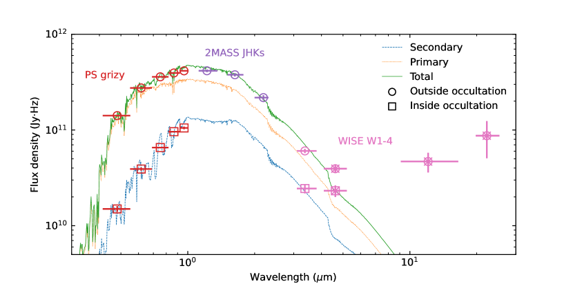
Figure 2: SEDs at different phases and the best-fit binary model. Observations from Pan-STARRS, 2MASS, and WISE are shown in red, purple, and pink, respectively. The extent of each point along the wavelength direction indicates the corresponding bandwidth. The data obtained outside-occultation phase is shown in circles, while the data obtained inside-occultation phase is shown in squares. Note that points with an additional cross are not used in the fitting process. The orange dotted and blue dashed and lines show the best-fit stellar SED model for the primary and secondary, respectively. The outside-occultation data are fitted by the summation of the two components, which is shown in green solid line.

3.1 Radial Velocity Modeling

We model the radial velocity data with a Keplerian model using the radvel package (Fulton et al., 2018). The RV curve of the primary star is given by

$$v_{\rm r}=K[\cos(\nu+\omega)+e\cos(\omega)]+\gamma.$$ (1)

Here $\gamma$, $\omega$, and $e$ are the systemic velocity, the argument of periastron, and eccentricity, respectively. The RV semi-amplitude, $K$, is given by

$$K \equiv\frac{2\pi}{P}\frac{a_{1}\sin i}{(1-e^{2})^{1/2}}$$ (2)

$$=51\left(\frac{P}{63\,\text{d}}\right)^{-1/3}\left(\frac{M_{1}}{M_{\odot}}\right)^{1/3}\times$$

$$\frac{q\sin i}{(1+q)^{2/3}(1-e^{2})^{1/2}}\,\text{km}\,\text{s}^{-1},$$

where $P$ is the binary period, $a_{1}$ is the semi-major axis of the primary star, $M_{1}$ is the mass of the primary star, $q\equiv M_{2}/M_{1}$ is the mass ratio of the binary, and $i$ is the inclination of the binary orbit. The true anomaly, $\nu$, is related to the eccentricity and the eccentric anomaly $E$ via

$$\nu =2\tan^{-1}\left(\sqrt{\frac{1+e}{1-e}}\tan\frac{E}{2}\right),$$ (3)

where $E$ is solved from the Kepler’s equation

$$E-e\sin E=\frac{2\pi}{P}(t-T_{\rm p}).$$ (4)

Here $T_{\rm P}$ is the time of pericenter passage.

We have fixed the orbital period to 63.358 days, which is the best-fit value in Zhu et al. (2022), as we do not expect to constrain $P$ from the sparse RV observations alone. We have nevertheless tested that the derived model parameters are not affected by any small change in the period value we use. The RV jitters of GTC and KPF observations are consistent with zero if included, so for simplicity we do not include the jitter term. We fit the systemic velocities for GTC and KPF data separately to compensate for the velocity offset between the two telescopes. Since there is only one data point from Magellan/FIRE, it is used for a sanity check and not included in the fitting. It aligns with the model prediction to within 1-$\sigma$, irrespective of whether we assume it shares the same velocity offset with GTC or KPF. As shown in the top panel of Figure 1, the first and last GTC observations are not included in the RV modeling. The former was observed during egress and the latter is a clear outlier. Therefore, we have in total six free parameters for 11 data points. We use emcee (Foreman-Mackey et al., 2013) to sample the posteriors of the model parameters. In total 100 walkers are used, with each drawing 7000 steps and the first 5000 steps removed as burn-in steps. The best-fit parameters with the associated uncertainties are given in Table 1, and the best-fit model is shown in the upper panel of Figure 1. The phase-folded RV model and data are also shown in Figure 3.

With $e=0.69\pm 0.08$ and $K=22\pm 4\,{\rm km~{}s}^{-1}$, Bernhard-2 is indeed a stellar binary with very eccentric orbit, thus resembling the key characteristics of the KH-15D system. We next model the system SEDs in order to determine the physical parameters of the binary stars.

3.2 Spectral Energy Distribution

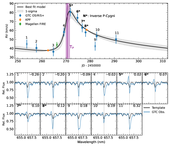
Figure 3: The phase folded RV fitting result (upper panel) and the corresponding GTC H-$\alpha$ profiles (lower panel). The description of data points and model in the upper panel is the same as Figure 1 except for the number above each GTC data point, which labels the observations in ascending phase order. Note that the bold numbers with asterisk are the observations with inverse P-Cygni H-$\alpha$ profile. The pericenter passage time is shown with the purple solid line, respectively. The purple shaded region indicates the fitting error of ${\rm T}_{\rm P}$. In the lower panels, we show the observed spectra as well as the single star template near the H$\alpha$ region with blue and black solid lines, respectively. The number on the upper left of each panel is the observation label in the upper panel, while the number on the upper right indicates the corresponding phase.

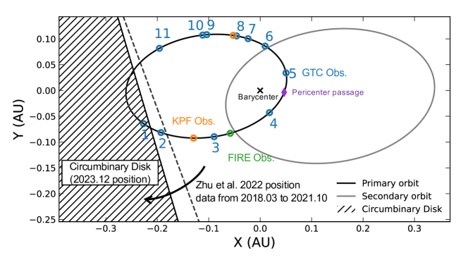
Figure 4: The sky-projected view of the binary orbital dynamics and the boundary of the occulting disk in the Bernhard-2 system. In order to illustrate the orbital characteristics and the change in the disk edge position, we only show the model with the best-fitting parameters. The hatched area shows the updated position of the disk edge from our new photometric observations (detailed in Section 2.3), whereas the dashed line indicates the edge position reported in Zhu et al. (2022), which utilized ZTF data collected over the period from 2018 to 2021. The black and gray ellipses represent the primary and secondary orbits, respectively, which are constructed using the best-fitting RV and stellar parameters, assuming an arbitrary longitude of the ascending node. The blue, orange, and green circles denote the positions of the primary star when the observations were conducted with GTC OSIRIS, KPF, and Magellan FIRE, respectively. Similar to Figure 3, the GTC observations are indexed according to the orbital phases.

We adopt the multi-band photometric data from Zhu et al. (2022) and conduct a spectral energy distribution (SED) fitting, in order to determine the physical parameters of the two stellar components. The data include grizy bands from Pan-STARRS1 (Chambers et al., 2016), JHK bands from 2MASS (Skrutskie et al., 2006), andW1 to W4 bands from WISE (Wright et al., 2010), ranging from $\sim$ 0.5 $\micron$ to $\sim$ 20 $\micron$ for both inside and outside the occultation. We include a minimum photometric accuracy of $0.03$ mag to account for the potential systematics between different surveys, which is added in quadrature to the reported photometric uncertainty to derive the total photometric error (see also El-Badry et al. 2024).

The SED of the Bernhard-2 system shows clear evidence for the NIR excess (Zhu et al., 2022), so in modeling the stellar SED, we have excluded the WISE W2 to W4 measurements. We have tested that the derived stellar parameters and the corresponding errors remain largely unchanged if the WISE W1 band is also excluded. Under our assumption of a fully opaque disk, the inside-occultation SED is produced by the secondary star alone, whereas the outside-occultation SED is the superposition of both stellar components. For the primary star, we have also included the spectroscopic measurements from Zhu et al. (2022), namely the effective temperature $T_{\rm eff}=4865\pm 85$ K and the surface gravity $\log g=4.37\pm 0.04$, and the parallax constraint of $0.34\pm 0.16$ mas from Gaia DR3 (Gaia Collaboration et al., 2023).

We modeled the stellar SED with the isochrones package (Morton, 2015). The isochrones package interpolates on the MESA Isochrones & Stellar Tracks (MIST) (Dotter, 2016; Choi et al., 2016) to predict stellar physical parameters. The magnitude of a star in a certain band is given by

$$m_{\rm B}=f({\rm EEP},\log{\rm age},{\rm[Fe/H]},d,A_{V}).$$ (5)

Here EEP is the equivalent evolution phase (Dotter, 2016), $d$ is the distance, and $A_{V}$ is the extinction. The standard Cardelli et al. (1989) extinction law with $R_{V}=3.1$ is assumed. The two stars in the binary share all properties except for the EEP parameter. The best-fit model is obtained by optimizing the total log-likelihood of all measurements, and again we use the emcee sampler (Foreman-Mackey et al., 2013) to sample the posterior and derive the uncertainties of the model parameters.

The result of the stellar SED fitting is also given in Table 1, and the corresponding stellar spectra generated with the best-fit stellar parameters are shown in Figure 2 with the dashed line. For a better illustration, we have used a spectra interpolator pystellibs to generate the spectra, and the empirical stellar spectra library BaSeL (v2.2, Lejeune et al., 1997, 1998) has been used.

Our results indicate that the binary is composed of an early K-type star of $\sim 1.1\,M_{\odot}$ and a late K-type star of $\sim 0.9\,M_{\odot}$ at a distance of $\sim 1.8\,$kpc. The stellar age is estimated to be around $20\,$Myr, in general consistent with the young nature of the system. The predicted flux ratio of the binary in the optical $r$ band is around 0.16, so the impact of the secondary star on the RV derivation of the primary star is limited. However, the flux ratio in the IR bands (e.g., $W1$) can be as large as $\sim 0.7$, which may be large enough to identify the secondary component directly.

When combined with the eccentricity and RV semi-amplitude measurements from RV modeling, the derived stellar masses allow us to constrain the inclination of the binary orbit. This yields $\sin{i}=0.58\pm 0.07$ and $i=36\pm 5^{\circ}$. Additionally, the binary separation can be derived through Kepler’s third law

$$a_{\rm bin}=0.4\ {\rm AU}\left(\frac{P_{\rm bin}}{63\ {\rm day}}\right)^{2/3}\left(\frac{M_{1}+M_{2}}{2\ M_{\sun}}\right)^{1/3}.$$ (6)

The near-IR excess is expected to originate from the circumbinary disk. A detailed modeling of the disk spectral energy distribution is not possible with the available observations, but as a start it is reasonable to believe that the radiation from the circumbinary disk peaks beyond $\sim 20\,\mu$m based on the WISE measurements. This corresponds to a blackbody temperature $\lesssim 140\,$K, which is the equilibrium temperature at a distance of $\gtrsim 4\,$au from the central binary. Therefore, the circumbinary disk in Bernhard-2 may extend out to several au, Similar to the prototype KH 15D system (Poon et al., 2021).

4 Discussion

In this paper, we present new spectroscopic and photometric observations of the Bernhard-2 system, which has been proposed as a KH 15D-like system. The spectroscopic observations confirm that Bernhard-2 is indeed a highly eccentric binary ($e=0.69\pm 0.08$), and the photometric behavior can only be explained by a circumbinary disk that is (potentially highly) misaligned relative to the binary orbit. Therefore, Bernhard-2 is a confirmed KH 15D-like system. The system configuration is illustrated in Figure 4. Through modeling the SEDs inside and outside the disk occultation, we determine the binary to be composed of two pre-main sequence K-dwarfs of $\sim 1.1\,M_{\odot}$ and $\sim 0.9\,M_{\odot}$, respectively.

he spectroscopic observations deliver more than the RV measurements. As shown in the lower panels of Figure 3, the H-$\alpha$ line profiles from GTC OSIRIS appear to be time-variable. In comparison with the model template, which is shown in black, the observed H-$\alpha$ lines are deeper and wider, and the depth and width vary with time. Similar to the KH 15D system (Hamilton et al., 2012), Bernhard-2 also shows an inverse P-Cygni profile in the H-$\alpha$ line at certain epochs. The blue-side emission component is clearly seen in epochs 5 and 6 and marginally visible in epochs 7 and 8. These epochs are close to the time of the pericenter passage, which is marked by the purple vertical line in Figure 3, consistent with the theoretical modelings that the pulsed accretion phenomenon is enhanced during or after the pericenter passage (e.g., Artymowicz & Lubow, 1996; Günther & Kley, 2002; de Val-Borro et al., 2011). Nevertheless, observations with higher S/N and resolutions are needed to better understand the behavior and origin of the H-$\alpha$ line variations.

Our new photometric observations show very clear deviation, most notably in the shortened occultation duration, from the model prediction based on the ZTF data. This may be indicating the ongoing precession of the circumbinary disk, similar to that seen in the prototype KH 15D system. Long-term photometric monitoring of Bernhard-2 is needed to better understand and constrain the dynamical evolution of this rare system.

Appendix A The RV Data

The RV measurements are provided in Table 2, in case they are needed for future analysis.

Table 2: The extracted RV for the Bernhard-2 system.

${\rm BJD}_{\rm TDB}-2460000$	RV (km/s)	Instrument
253.7506	$50\pm 5$	GTC OSIRIS
257.7451	$46\pm 5$	GTC OSIRIS
264.7550	$42\pm 5$	GTC OSIRIS
271.7586	$86\pm 5$	GTC OSIRIS
274.7413	$79\pm 5$	GTC OSIRIS
276.7037	$68\pm 5$	GTC OSIRIS
282.6777	$59\pm 5$	GTC OSIRIS
290.6924	$55\pm 5$	GTC OSIRIS
325.9211	$37.67\pm 0.10$	KPF
329.5608	$44\pm 3$	Magellen FIRE
332.5107	$64\pm 5$	GTC OSIRIS
341.4479	$63\pm 5$	GTC OSIRIS
341.8599	$60.68\pm 0.10$	KPF
345.4235	$48\pm 5$	GTC OSIRIS

References

- Aly et al. (2015) Aly, H., Dehnen, W., Nixon, C., & King, A. 2015, MNRAS, 449, 65, doi: 10.1093/mnras/stv128
- Aronow et al. (2018) Aronow, R. A., Herbst, W., Hughes, A. M., Wilner, D. J., & Winn, J. N. 2018, AJ, 155, 47, doi: 10.3847/1538-3881/aa9ed7
- Artymowicz & Lubow (1996) Artymowicz, P., & Lubow, S. H. 1996, ApJ, 467, L77, doi: 10.1086/310200
- Arulanantham et al. (2016) Arulanantham, N. A., Herbst, W., Cody, A. M., et al. 2016, The Astronomical Journal, 151, 90, doi: 10.3847/0004-6256/151/4/90
- Astropy Collaboration et al. (2013) Astropy Collaboration, Robitaille, T. P., Tollerud, E. J., et al. 2013, A&A, 558, A33, doi: 10.1051/0004-6361/201322068
- Astropy Collaboration et al. (2018) Astropy Collaboration, Price-Whelan, A. M., Sipőcz, B. M., et al. 2018, AJ, 156, 123, doi: 10.3847/1538-3881/aabc4f
- Astropy Collaboration et al. (2022) Astropy Collaboration, Price-Whelan, A. M., Lim, P. L., et al. 2022, ApJ, 935, 167, doi: 10.3847/1538-4357/ac7c74
- Bellm et al. (2019) Bellm, E. C., Kulkarni, S. R., Barlow, T., et al. 2019, PASP, 131, 068003, doi: 10.1088/1538-3873/ab0c2a
- Blanco-Cuaresma (2019) Blanco-Cuaresma, S. 2019, MNRAS, 486, 2075, doi: 10.1093/mnras/stz549
- Brinch et al. (2016) Brinch, C., Jørgensen, J. K., Hogerheijde, M. R., Nelson, R. P., & Gressel, O. 2016, ApJ, 830, L16, doi: 10.3847/2041-8205/830/1/L16
- Capelo et al. (2012) Capelo, H. L., Herbst, W., Leggett, S. K., Hamilton, C. M., & Johnson, J. A. 2012, ApJ, 757, L18, doi: 10.1088/2041-8205/757/1/L18
- Cardelli et al. (1989) Cardelli, J. A., Clayton, G. C., & Mathis, J. S. 1989, ApJ, 345, 245, doi: 10.1086/167900
- Cepa et al. (2013) Cepa, J., Bongiovanni, A., Pérez García, A. M., et al. 2013, in Highlights of Spanish Astrophysics VII, ed. J. C. Guirado, L. M. Lara, V. Quilis, & J. Gorgas, 868–873
- Chambers et al. (2016) Chambers, K. C., Magnier, E. A., Metcalfe, N., et al. 2016, arXiv e-prints, arXiv:1612.05560, doi: 10.48550/arXiv.1612.05560
- Chiang & Murray-Clay (2004) Chiang, E. I., & Murray-Clay, R. A. 2004, ApJ, 607, 913, doi: 10.1086/383522
- Choi et al. (2016) Choi, J., Dotter, A., Conroy, C., et al. 2016, ApJ, 823, 102, doi: 10.3847/0004-637X/823/2/102
- Cuello & Giuppone (2019) Cuello, N., & Giuppone, C. A. 2019, A&A, 628, A119, doi: 10.1051/0004-6361/201833976
- Dai et al. (2024) Dai, F., Howard, A. W., Halverson, S., et al. 2024, AJ, 168, 101, doi: 10.3847/1538-3881/ad5a7d
- de Val-Borro et al. (2011) de Val-Borro, M., Gahm, G. F., Stempels, H. C., & Pepliński, A. 2011, MNRAS, 413, 2679, doi: 10.1111/j.1365-2966.2011.18339.x
- Dotter (2016) Dotter, A. 2016, ApJS, 222, 8, doi: 10.3847/0067-0049/222/1/8
- Doyle et al. (2011) Doyle, L. R., Carter, J. A., Fabrycky, D. C., et al. 2011, Science, 333, 1602, doi: 10.1126/science.1210923
- El-Badry et al. (2024) El-Badry, K., Simon, J. D., Reggiani, H., et al. 2024, A $1.9\,M_{\odot}$ Neutron Star Candidate in a 2-Year Orbit, arXiv. https://arxiv.org/abs/2402.06722
- Fernández-López et al. (2017) Fernández-López, M., Zapata, L. A., & Gabbasov, R. 2017, ApJ, 845, 10, doi: 10.3847/1538-4357/aa7d51
- Foreman-Mackey et al. (2013) Foreman-Mackey, D., Hogg, D. W., Lang, D., & Goodman, J. 2013, Publications of the Astronomical Society of the Pacific, 125, 306, doi: 10.1086/670067
- Fulton et al. (2018) Fulton, B. J., Petigura, E. A., Blunt, S., & Sinukoff, E. 2018, Publications of the Astronomical Society of the Pacific, 130, 044504, doi: 10.1088/1538-3873/aaaaa8
- Gaia Collaboration et al. (2023) Gaia Collaboration, Vallenari, A., Brown, A. G. A., et al. 2023, A&A, 674, A1, doi: 10.1051/0004-6361/202243940
- García Soto et al. (2020) García Soto, A., Ali, A., Newmark, A., et al. 2020, AJ, 159, 135, doi: 10.3847/1538-3881/ab6efd
- Gibson et al. (2016) Gibson, S. R., Howard, A. W., Marcy, G. W., et al. 2016, in Society of Photo-Optical Instrumentation Engineers (SPIE) Conference Series, Vol. 9908, Ground-based and Airborne Instrumentation for Astronomy VI, ed. C. J. Evans, L. Simard, & H. Takami, 990870, doi: 10.1117/12.2233334
- Gibson et al. (2018) Gibson, S. R., Howard, A. W., Roy, A., et al. 2018, in Society of Photo-Optical Instrumentation Engineers (SPIE) Conference Series, Vol. 10702, Ground-based and Airborne Instrumentation for Astronomy VII, ed. C. J. Evans, L. Simard, & H. Takami, 107025X, doi: 10.1117/12.2311565
- Gibson et al. (2020) Gibson, S. R., Howard, A. W., Rider, K., et al. 2020, in Society of Photo-Optical Instrumentation Engineers (SPIE) Conference Series, Vol. 11447, Ground-based and Airborne Instrumentation for Astronomy VIII, ed. C. J. Evans, J. J. Bryant, & K. Motohara, 1144742, doi: 10.1117/12.2561783
- Günther & Kley (2002) Günther, R., & Kley, W. 2002, A&A, 387, 550, doi: 10.1051/0004-6361:20020407
- Hamilton et al. (2012) Hamilton, C. M., Johns-Krull, C. M., Mundt, R., Herbst, W., & Winn, J. N. 2012, The Astrophysical Journal, 751, 147, doi: 10.1088/0004-637X/751/2/147
- Hamilton et al. (2005) Hamilton, C. M., Herbst, W., Vrba, F. J., et al. 2005, AJ, 130, 1896, doi: 10.1086/432667
- Husser et al. (2013) Husser, T. O., Wende-von Berg, S., Dreizler, S., et al. 2013, A&A, 553, A6, doi: 10.1051/0004-6361/201219058
- Johnson et al. (2004) Johnson, J. A., Marcy, G. W., Hamilton, C. M., Herbst, W., & Johns-Krull, C. M. 2004, The Astronomical Journal, 128, 1265, doi: 10.1086/422735
- Johnson et al. (2005) Johnson, J. A., Winn, J. N., Rampazzi, F., et al. 2005, AJ, 129, 1978, doi: 10.1086/428597
- Kearns & Herbst (1998) Kearns, K. E., & Herbst, W. 1998, AJ, 116, 261, doi: 10.1086/300426
- Kennedy et al. (2012) Kennedy, G. M., Wyatt, M. C., Sibthorpe, B., et al. 2012, MNRAS, 421, 2264, doi: 10.1111/j.1365-2966.2012.20448.x
- Kennedy et al. (2019) Kennedy, G. M., Matrà, L., Facchini, S., et al. 2019, Nature Astronomy, 3, 230, doi: 10.1038/s41550-018-0667-x
- Kenworthy et al. (2022) Kenworthy, M. A., González Picos, D., Elizondo, E., et al. 2022, A&A, 666, A61, doi: 10.1051/0004-6361/202243441
- Köhler (2011) Köhler, R. 2011, A&A, 530, A126, doi: 10.1051/0004-6361/201016327
- Kostov et al. (2020) Kostov, V. B., Orosz, J. A., Feinstein, A. D., et al. 2020, AJ, 159, 253, doi: 10.3847/1538-3881/ab8a48
- Lacour et al. (2016) Lacour, S., Biller, B., Cheetham, A., et al. 2016, A&A, 590, A90, doi: 10.1051/0004-6361/201527863
- Lejeune et al. (1997) Lejeune, T., Cuisinier, F., & Buser, R. 1997, A&AS, 125, 229, doi: 10.1051/aas:1997373
- Lejeune et al. (1998) —. 1998, A&AS, 130, 65, doi: 10.1051/aas:1998405
- Lubow & Martin (2018) Lubow, S. H., & Martin, R. G. 2018, MNRAS, 473, 3733, doi: 10.1093/mnras/stx2643
- Maffei et al. (2005) Maffei, P., Ciprini, S., & Tosti, G. 2005, MNRAS, 357, 1059, doi: 10.1111/j.1365-2966.2005.08724.x
- Martin & Lubow (2017) Martin, R. G., & Lubow, S. H. 2017, ApJ, 835, L28, doi: 10.3847/2041-8213/835/2/L28
- Masci et al. (2019) Masci, F. J., Laher, R. R., Rusholme, B., et al. 2019, PASP, 131, 018003, doi: 10.1088/1538-3873/aae8ac
- Morton (2000) Morton, D. C. 2000, ApJS, 130, 403, doi: 10.1086/317349
- Morton (2015) Morton, T. D. 2015, isochrones: Stellar model grid package, Astrophysics Source Code Library, record ascl:1503.010
- Poon et al. (2021) Poon, M., Zanazzi, J. J., & Zhu, W. 2021, Monthly Notices of the Royal Astronomical Society, 503, 1599, doi: 10.1093/mnras/stab575
- Prochaska et al. (2020) Prochaska, J. X., Hennawi, J. F., Westfall, K. B., et al. 2020, Journal of Open Source Software, 5, 2308, doi: 10.21105/joss.02308
- Prochaska et al. (2020) Prochaska, J. X., Hennawi, J., Cooke, R., et al. 2020, pypeit/PypeIt: Release 1.0.0, v1.0.0, Zenodo, doi: 10.5281/zenodo.3743493
- Silvia & Agol (2008) Silvia, D. W., & Agol, E. 2008, ApJ, 681, 1377, doi: 10.1086/588545
- Simcoe et al. (2008) Simcoe, R. A., Burgasser, A. J., Bernstein, R. A., et al. 2008, in Society of Photo-Optical Instrumentation Engineers (SPIE) Conference Series, Vol. 7014, Ground-based and Airborne Instrumentation for Astronomy II, ed. I. S. McLean & M. M. Casali, 70140U, doi: 10.1117/12.790414
- Skrutskie et al. (2006) Skrutskie, M. F., Cutri, R. M., Stiening, R., et al. 2006, AJ, 131, 1163, doi: 10.1086/498708
- Smallwood et al. (2020) Smallwood, J. L., Franchini, A., Chen, C., et al. 2020, MNRAS, 494, 487, doi: 10.1093/mnras/staa654
- Winn et al. (2006) Winn, J. N., Hamilton, C. M., Herbst, W. J., et al. 2006, The Astrophysical Journal, 644, 510, doi: 10.1086/503417
- Winn et al. (2004) Winn, J. N., Holman, M. J., Johnson, J. A., Stanek, K. Z., & Garnavich, P. M. 2004, ApJ, 603, L45, doi: 10.1086/383089
- Wright et al. (2010) Wright, E. L., Eisenhardt, P. R. M., Mainzer, A. K., et al. 2010, AJ, 140, 1868, doi: 10.1088/0004-6256/140/6/1868
- Zanazzi & Lai (2018) Zanazzi, J. J., & Lai, D. 2018, MNRAS, 473, 603, doi: 10.1093/mnras/stx2375
- Zhu et al. (2022) Zhu, W., Bernhard, K., Dai, F., et al. 2022, The Astrophysical Journal Letters, 933, L21, doi: 10.3847/2041-8213/ac7b2d